Autoregressive Models - Stanford...
33
Autoregressive Models Stefano Ermon, Aditya Grover Stanford University Lecture 3 Stefano Ermon, Aditya Grover (AI Lab) Deep Generative Models Lecture 3 1 / 31
Transcript of Autoregressive Models - Stanford...
Autoregressive Models
Stefano Ermon, Aditya Grover
Stanford University
Lecture 3
Stefano Ermon, Aditya Grover (AI Lab) Deep Generative Models Lecture 3 1 / 31

Learning a generative model
We are given a training set of examples, e.g., images of dogs
We want to learn a probability distribution p(x) over images x such that
1 Generation: If we sample xnew ∼ p(x), xnew should look like a dog(sampling)
2 Density estimation: p(x) should be high if x looks like a dog, and lowotherwise (anomaly detection)
3 Unsupervised representation learning: We should be able to learnwhat these images have in common, e.g., ears, tail, etc. (features)
First question: how to represent p(x). Second question: how to learn it.
Stefano Ermon, Aditya Grover (AI Lab) Deep Generative Models Lecture 3 2 / 31

Recap: Bayesian networks vs neural models
Using Chain Rule
p(x1, x2, x3, x4) = p(x1)p(x2 | x1)p(x3 | x1, x2)p(x4 | x1, x2, x3)
Fully General, no assumptions needed (exponential size, no free lunch)
Bayes Net
p(x1, x2, x3, x4) ≈ pCPT(x1)pCPT(x2 | x1)pCPT(x3 |��x1, x2)pCPT(x4 | x1,���x2, x3)
Assumes conditional independencies; tabular representations via conditionalprobability tables (CPT)
Neural Models
p(x1, x2, x3, x4) ≈ p(x1)p(x2 | x1)pNeural(x3 | x1, x2)pNeural(x4 | x1, x2, x3)
Assumes specific functional form for the conditionals. A sufficiently deepneural net can approximate any function.
Stefano Ermon, Aditya Grover (AI Lab) Deep Generative Models Lecture 3 3 / 31

Neural Models for classification
Setting: binary classification of Y ∈ {0, 1} given input features X ∈ {0, 1}n
For classification, we care about p(Y | x), and assume that
p(Y = 1 | x;α) = f (x,α)
Logistic regression: let z(α, x) = α0 +∑n
i=1 αixi .plogit(Y = 1 | x;α) = σ(z(α, x)), where σ(z) = 1/(1 + e−z)
Non-linear dependence: let h(A,b, x) be a non-linear transformation of the
input features. pNeural(Y = 1 | x;α,A,b) = σ(α0 +∑h
i=1 αihi )
More flexibleMore parameters: A,b,αRepeat multiple times to get a multilayer perceptron (neural network)
Stefano Ermon, Aditya Grover (AI Lab) Deep Generative Models Lecture 3 4 / 31

Motivating Example: MNIST
Given: a dataset D of handwritten digits (binarized MNIST)
Each image has n = 28× 28 = 784 pixels. Each pixel can either beblack (0) or white (1).
Goal: Learn a probability distribution p(x) = p(x1, · · · , x784) overx ∈ {0, 1}784 such that when x ∼ p(x), x looks like a digit
Two step process:1 Parameterize a model family {pθ(x), θ ∈ Θ} [This lecture]2 Search for model parameters θ based on training data D [Next lecture]
Stefano Ermon, Aditya Grover (AI Lab) Deep Generative Models Lecture 3 5 / 31

Autoregressive Models
We can pick an ordering of all the random variables, i.e., raster scanordering of pixels from top-left (X1) to bottom-right (Xn=784)
Without loss of generality, we can use chain rule for factorization
p(x1, · · · , x784) = p(x1)p(x2 | x1)p(x3 | x1, x2) · · · p(xn | x1, · · · , xn−1)
Some conditionals are too complex to be stored in tabular form. Instead, weassume
p(x1, · · · , x784) = pCPT(x1;α1)plogit(x2 | x1;α2)plogit(x3 | x1, x2;α3) · · ·plogit(xn | x1, · · · , xn−1;αn)
More explicitly
pCPT(X1 = 1;α1) = α1, p(X1 = 0) = 1− α1
plogit(X2 = 1 | x1;α2) = σ(α20 + α2
1x1)plogit(X3 = 1 | x1, x2;α3) = σ(α3
0 + α31x1 + α3
2x2)
Note: This is a modeling assumption. We are using parameterizedfunctions (e.g., logistic regression above) to predict next pixel given all theprevious ones. Called autoregressive model.
Stefano Ermon, Aditya Grover (AI Lab) Deep Generative Models Lecture 3 6 / 31
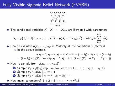
Fully Visible Sigmoid Belief Network (FVSBN)
The conditional variables Xi | X1, · · · ,Xi−1 are Bernoulli with parameters
x̂i = p(Xi = 1|x1, · · · , xi−1;αi ) = p(Xi = 1|x<i ;αi ) = σ(αi
0 +i−1∑j=1
αijxj)
How to evaluate p(x1, · · · , x784)? Multiply all the conditionals (factors)In the above example:
p(X1 = 0,X2 = 1,X3 = 1,X4 = 0) = (1− x̂1)× x̂2 × x̂3 × (1− x̂4)
= (1− x̂1)× x̂2(X1 = 0)× x̂3(X1 = 0,X2 = 1)× (1− x̂4(X1 = 0,X2 = 1,X3 = 1))
How to sample from p(x1, · · · , x784)?1 Sample x1 ∼ p(x1) (np.random.choice([1,0],p=[x̂1, 1− x̂1]))2 Sample x2 ∼ p(x2 | x1 = x1)3 Sample x3 ∼ p(x3 | x1 = x1, x2 = x2) · · ·
How many parameters? 1 + 2 + 3 + · · ·+ n ≈ n2/2Stefano Ermon, Aditya Grover (AI Lab) Deep Generative Models Lecture 3 7 / 31
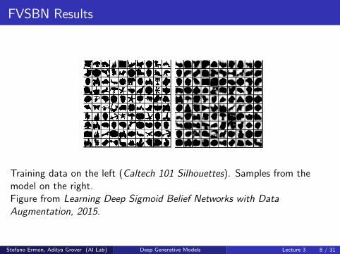
FVSBN Results
Training data on the left (Caltech 101 Silhouettes). Samples from themodel on the right.Figure from Learning Deep Sigmoid Belief Networks with DataAugmentation, 2015.
Stefano Ermon, Aditya Grover (AI Lab) Deep Generative Models Lecture 3 8 / 31

NADE: Neural Autoregressive Density Estimation
To improve model: use one layer neural network instead of logistic regression
hi = σ(Aix<i + ci )
x̂i = p(xi |x1, · · · , xi−1;Ai , ci ,αi , bi︸ ︷︷ ︸parameters
) = σ(αihi + bi )
For example h2 = σ
( ...
)︸︷︷︸A2
x1 +(
...
)︸︷︷︸c2
h3 = σ
( ......
)︸ ︷︷ ︸
A3
( x1x2 ) +
(...
)︸︷︷︸c3
Stefano Ermon, Aditya Grover (AI Lab) Deep Generative Models Lecture 3 9 / 31

NADE: Neural Autoregressive Density Estimation
Tie weights to reduce the number of parameters and speed up computation(see blue dots in the figure):
hi = σ(W·,<ix<i + c)
x̂i = p(xi |x1, · · · , xi−1) = σ(αihi + bi )
For example h2 = σ
...
w1
.
.
.
︸ ︷︷ ︸
A2
x1
h3 = σ
...
.
.
.w1 w2
.
.
.
.
.
.
︸ ︷︷ ︸
A3
(x1x2
)
h4 = σ
...
.
.
.
.
.
.w1 w2 w3
.
.
.
.
.
.
.
.
.
︸ ︷︷ ︸
A3
( x1x2x3
)
If hi ∈ Rd , how many total parameters? Linear in n: weights W ∈ Rd×n,biases c ∈ Rd , and n logistic regression coefficient vectors αi , bi ∈ Rd+1.Probability is evaluated in O(nd).
Stefano Ermon, Aditya Grover (AI Lab) Deep Generative Models Lecture 3 10 / 31

NADE results
Samples on the left. Conditional probabilities x̂i on the right.Figure from The Neural Autoregressive Distribution Estimator, 2011.
Stefano Ermon, Aditya Grover (AI Lab) Deep Generative Models Lecture 3 11 / 31

General discrete distributions
How to model non-binary discrete random variables Xi ∈ {1, · · · ,K}? E.g., pixelintensities varying from 0 to 255One solution: Let x̂ i parameterize a categorical distribution
hi = σ(W·,<ix<i + c)
p(xi |x1, · · · , xi−1) = Cat(p1i , · · · , pK
i )
x̂ i = (p1i , · · · , pK
i ) = softmax(Xihi + bi )
Softmax generalizes the sigmoid/logistic function σ(·) and transforms a vector ofK numbers into a vector of K probabilities (non-negative, sum to 1).
softmax(a) = softmax(a1, · · · , aK ) =
(exp(a1)∑i exp(ai )
, · · · , exp(aK )∑i exp(ai )
)In numpy: np.exp(a)/np.sum(np.exp(a))
Stefano Ermon, Aditya Grover (AI Lab) Deep Generative Models Lecture 3 12 / 31

RNADE
How to model continuous random variables Xi ∈ R? E.g., speech signalsSolution: let x̂ i parameterize a continuous distributionE.g., uniform mixture of K Gaussians
Stefano Ermon, Aditya Grover (AI Lab) Deep Generative Models Lecture 3 13 / 31

RNADE
How to model continuous random variables Xi ∈ R? E.g., speech signalsSolution: let x̂ i parameterize a continuous distributionE.g., In a mixture of K Gaussians,
p(xi |x1, · · · , xi−1) =K∑j=1
1
KN (xi ;µ
ji , σ
ji )
hi = σ(W·,<ix<i + c)
x̂ i = (µ1i , · · · , µK
i , σ1i , · · · , σK
i ) = f (hi )
x̂ i defines the mean and stddev of each Gaussian (µji , σ
ji ). Can use exponential
exp(·) to ensure stddev is positiveStefano Ermon, Aditya Grover (AI Lab) Deep Generative Models Lecture 3 14 / 31

Autoregressive models vs. autoencoders
On the surface, FVSBN and NADE look similar to an autoencoder:
an encoder e(·). E.g., e(x) = σ(W 2(W 1x + b1) + b2)
a decoder such that d(e(x)) ≈ x . E.g., d(h) = σ(Vh + c).
Loss functionBinary r.v.: min
W 1,W 2,b1,b2,V ,c
∑x∈D
∑i
−xi log x̂i − (1 − xi ) log(1 − x̂i )
Continuous r.v.: minW 1,W 2,b1,b2,V ,c
∑x∈D
∑i
(xi − x̂i )2
e and d are constrained so that we don’t learn identity mappings. Hope thate(x) is a meaningful, compressed representation of x (feature learning)
A vanilla autoencoder is not a generative model: it does not define adistribution over x we can sample from to generate new data points.
Stefano Ermon, Aditya Grover (AI Lab) Deep Generative Models Lecture 3 15 / 31

Autoregressive autoencoders
On the surface, FVSBN and NADE look similar to an autoencoder. Can weget a generative model from an autoencoder?
We need to make sure it corresponds to a valid Bayesian Network (DAGstructure), i.e., we need an ordering. If the ordering is 1, 2, 3, then:
x̂1 cannot depend on any input x . Then at generation time we don’tneed any input to get startedx̂2 can only depend on x1· · ·
Bonus: we can use a single neural network (with n outputs) to produce allthe parameters. In contrast, NADE requires n passes. Much more efficienton modern hardware.
Stefano Ermon, Aditya Grover (AI Lab) Deep Generative Models Lecture 3 16 / 31
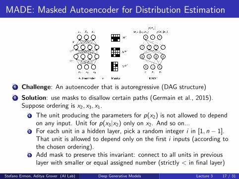
MADE: Masked Autoencoder for Distribution Estimation
1 Challenge: An autoencoder that is autoregressive (DAG structure)
2 Solution: use masks to disallow certain paths (Germain et al., 2015).Suppose ordering is x2, x3, x1.
1 The unit producing the parameters for p(x2) is not allowed to dependon any input. Unit for p(x3|x2) only on x2. And so on...
2 For each unit in a hidden layer, pick a random integer i in [1, n − 1].That unit is allowed to depend only on the first i inputs (according tothe chosen ordering).
3 Add mask to preserve this invariant: connect to all units in previouslayer with smaller or equal assigned number (strictly < in final layer)
Stefano Ermon, Aditya Grover (AI Lab) Deep Generative Models Lecture 3 17 / 31

RNN: Recurrent Neural Nets
Challenge: model p(xt |x1:t−1;αt). “History” x1:t−1 keeps getting longer.Idea: keep a summary and recursively update it
Summary update rule: ht+1 = tanh(Whhht + Wxhxt+1)
Prediction: ot+1 = Whyht+1
Summary initalization: h0 = b0
1 Hidden layer ht is a summary of the inputs seen till time t2 Output layer ot−1 specifies parameters for conditional p(xt | x1:t−1)3 Parameterized by b0 (initialization), and matrices Whh,Wxh,Why .
Constant number of parameters w.r.t n!Stefano Ermon, Aditya Grover (AI Lab) Deep Generative Models Lecture 3 18 / 31

Example: Character RNN (from Andrej Karpathy)
1 Suppose xi ∈ {h, e, l , o}. Use one-hot encoding:h encoded as [1, 0, 0, 0], e encoded as [0, 1, 0, 0], etc.
2 Autoregressive: p(x = hello) = p(x1 = h)p(x2 = e|x1 = h)p(x3 =l |x1 = h, x2 = e) · · · p(x5 = o|x1 = h, x2 = e, x3 = l , x4 = l)
3 For example,
p(x2 = e|x1 = h) = softmax(o1) =exp(2.2)
exp(1.0) + · · ·+ exp(4.1)
o1 = Whyh1
h1 = tanh(Whhh0 + Wxhx1)
Stefano Ermon, Aditya Grover (AI Lab) Deep Generative Models Lecture 3 19 / 31

RNN: Recursive Neural Nets
Pros:
1 Can be applied to sequences of arbitrary length.
2 Very general: For every computable function, there exists a finiteRNN that can compute it
Cons:
1 Still requires an ordering
2 Sequential likelihood evaluation (very slow for training)
3 Sequential generation (unavoidable in an autoregressive model)
4 Can be difficult to train (vanishing/exploding gradients)
Stefano Ermon, Aditya Grover (AI Lab) Deep Generative Models Lecture 3 20 / 31

Example: Character RNN (from Andrej Karpathy)
Train 3-layer RNN with 512 hidden nodes on all the works of Shakespeare.Then sample from the model:
KING LEAR: O, if you were a feeble sight, the courtesy of your law,Your sight and several breath, will wear the godsWith his heads, and my hands are wonder’d at the deeds,So drop upon your lordship’s head, and your opinionShall be against your honour.
Note: generation happens character by character. Needs to learn validwords, grammar, punctuation, etc.
Stefano Ermon, Aditya Grover (AI Lab) Deep Generative Models Lecture 3 21 / 31
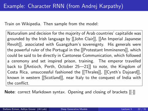
Example: Character RNN (from Andrej Karpathy)
Train on Wikipedia. Then sample from the model:
Naturalism and decision for the majority of Arab countries’ capitalide wasgrounded by the Irish language by [[John Clair]], [[An Imperial JapaneseRevolt]], associated with Guangzham’s sovereignty. His generals werethe powerful ruler of the Portugal in the [[Protestant Immineners]], whichcould be said to be directly in Cantonese Communication, which followeda ceremony and set inspired prison, training. The emperor travelledback to [[Antioch, Perth, October 25—21]] to note, the Kingdom ofCosta Rica, unsuccessful fashioned the [[Thrales]], [[Cynth’s Dajoard]],known in western [[Scotland]], near Italy to the conquest of India withthe conflict.
Note: correct Markdown syntax. Opening and closing of brackets [[·]]
Stefano Ermon, Aditya Grover (AI Lab) Deep Generative Models Lecture 3 22 / 31

Example: Character RNN (from Andrej Karpathy)
Train on Wikipedia. Then sample from the model:
{ { cite journal — id=Cerling Nonforest Depart-ment—format=Newlymeslated—none } }”www.e-complete”.”’See also”’: [[List of ethical consent processing]]
== See also ==*[[Iender dome of the ED]]*[[Anti-autism]]
== External links==* [http://www.biblegateway.nih.gov/entrepre/ Website of the WorldFestival. The labour of India-county defeats at the Ripper of CaliforniaRoad.]
Stefano Ermon, Aditya Grover (AI Lab) Deep Generative Models Lecture 3 23 / 31

Example: Character RNN (from Andrej Karpathy)
Train on data set of baby names. Then sample from the model:
Rudi Levette Berice Lussa Hany Mareanne Chrestina Carissy MarylenHammine Janye Marlise Jacacrie Hendred Romand Charienna NenottoEtte Dorane Wallen Marly Darine Salina Elvyn Ersia Maralena Minoria El-lia Charmin Antley Nerille Chelon Walmor Evena Jeryly Stachon CharisaAllisa Anatha Cathanie Geetra Alexie Jerin Cassen Herbett Cossie Ve-len Daurenge Robester Shermond Terisa Licia Roselen Ferine Jayn LusineCharyanne Sales Sanny Resa Wallon Martine Merus Jelen Candica WallinTel Rachene Tarine Ozila Ketia Shanne Arnande Karella Roselina AlessiaChasty Deland Berther Geamar Jackein Mellisand Sagdy Nenc LessieRasemy Guen Gavi Milea Anneda Margoris Janin Rodelin Zeanna ElyneJanah Ferzina Susta Pey Castina
Stefano Ermon, Aditya Grover (AI Lab) Deep Generative Models Lecture 3 24 / 31

Pixel RNN (Oord et al., 2016)
1 Model images pixel by pixel using raster scan order
2 Each pixel conditional p(xt | x1:t−1) needs to specify 3 colors
p(xt | x1:t−1) = p(x redt | x1:t−1)p(x
greent | x1:t−1, x
redt )p(xblue
t | x1:t−1, xredt , xgreen
t )
and each conditional is a categorical random variable with 256 possiblevalues
3 Conditionals modeled using RNN variants. LSTMs + masking (like MADE)
Stefano Ermon, Aditya Grover (AI Lab) Deep Generative Models Lecture 3 25 / 31

Pixel RNN
Results on downsampled ImageNet. Very slow: sequential likelihoodevaluation.
Stefano Ermon, Aditya Grover (AI Lab) Deep Generative Models Lecture 3 26 / 31

Convolutional Architectures
Convolutions are natural for image data and easy to parallelize on modernhardware.
Stefano Ermon, Aditya Grover (AI Lab) Deep Generative Models Lecture 3 27 / 31

PixelCNN (Oord et al., 2016)
Idea: Use convolutional architecture to predict next pixel given context (aneighborhood of pixels).Challenge: Has to be autoregressive. Masked convolutions preserve raster scanorder. Additional masking for colors order.
Stefano Ermon, Aditya Grover (AI Lab) Deep Generative Models Lecture 3 28 / 31

PixelCNN
Samples from the model trained on Imagenet (32× 32 pixels). Similarperformance to PixelRNN, but much faster.
Stefano Ermon, Aditya Grover (AI Lab) Deep Generative Models Lecture 3 29 / 31

Application in Adversarial Attacks and Anomaly detection
Machine learning methods are vulnerable to adversarial examples
Can we detect them?
Stefano Ermon, Aditya Grover (AI Lab) Deep Generative Models Lecture 3 30 / 31

PixelDefend (Song et al., 2018)
Train a generative model p(x) on clean inputs (PixelCNN)
Given a new input x , evaluate p(x)
Adversarial examples are significantly less likely under p(x)
Stefano Ermon, Aditya Grover (AI Lab) Deep Generative Models Lecture 3 31 / 31

WaveNet (Oord et al., 2016)
State of the art model for speech:
Dilated convolutions increase the receptive field: kernel only touches thesignal at every 2d entries.
Stefano Ermon, Aditya Grover (AI Lab) Deep Generative Models Lecture 3 32 / 31

Summary of Autoregressive Models
Easy to sample from1 Sample x0 ∼ p(x0)2 Sample x1 ∼ p(x1 | x0 = x0)3 · · ·
Easy to compute probability p(x = x)1 Compute p(x0 = x0)2 Compute p(x1 = x1 | x0 = x0)3 Multiply together (sum their logarithms)4 · · ·5 Ideally, can compute all these terms in parallel for fast training
Easy to extend to continuous variables. For example, can chooseGaussian conditionals p(xt | x<t) = N (µθ(x<t),Σθ(x<t)) or mixtureof logistics
No natural way to get features, cluster points, do unsupervisedlearning
Next: learning
Stefano Ermon, Aditya Grover (AI Lab) Deep Generative Models Lecture 3 33 / 31