AUTOPILOT AND GUIDANCE FOR ANTI-TANK IMAGING · PDF fileAn anti-tank guided missile is a...
130
i AUTOPILOT AND GUIDANCE FOR ANTI-TANK IMAGING INFRARED GUIDED MISSILES A THESIS SUBMITTED TO THE GRADUATE SCHOOL OF NATURAL AND APPLIED SCIENCES OF MIDDLE EAST TECHNICAL UNIVERSITY BY ALİ ERDEM ÖZCAN IN PARTIAL FULFILLMENT OF THE REQUIREMENTS FOR THE DEGREE OF MASTER OF SCIENCE IN ELECTRICAL AND ELECTRONICS ENGINEERING OCTOBER 2008
Transcript of AUTOPILOT AND GUIDANCE FOR ANTI-TANK IMAGING · PDF fileAn anti-tank guided missile is a...
i
AUTOPILOT AND GUIDANCE FOR ANTI-TANK IMAGING INFRARED GUIDED
MISSILES
A THESIS SUBMITTED TO THE GRADUATE SCHOOL OF NATURAL AND APPLIED SCIENCES
OF MIDDLE EAST TECHNICAL UNIVERSITY
BY
ALİ ERDEM ÖZCAN
IN PARTIAL FULFILLMENT OF THE REQUIREMENTS FOR
THE DEGREE OF MASTER OF SCIENCE IN
ELECTRICAL AND ELECTRONICS ENGINEERING
OCTOBER 2008

ii
Approval of the thesis:
AUTOPILOT AND GUIDANCE FOR ANTI-TANK IMAGING INFRARED GUIDED MISSILES
submitted by ALİ ERDEM ÖZCAN in partial fulfillment of the requirements for the degree of Master of Science in Electrical and Electronics Engineering Department, Middle East Technical University by, Prof. Dr. Canan Özgen __________ Dean, Graduate School of Natural and Applied Sciences Prof. Dr. İsmet Erkmen __________ Head of Department, Electrical and Electronics Engineering Prof. Dr. Kemal Leblebicioğlu __________ Supervisor, Electrical and Electronics Engineering Dept., METU Examining Committee Members: Prof. Dr. Mübeccel Demirekler ____________ Electrical and Electronics Engineering Dept., METU Prof. Dr. Kemal Leblebicioğlu ____________ Electrical and Electronics Engineering Dept., METU Prof. Dr. Gözde Bozdağı Akar ____________ Electrical and Electronics Engineering Dept., METU Assoc. Prof. Dr. Aydın Alatan ____________ Electrical and Electronics Engineering Dept., METU M. Sc. Emre Turgay ____________ Image Processing Dept., ASELSAN
Date: _____________

iii
I hereby declare that all information in this document has been obtained and presented in accordance with academic rules and ethical conduct. I also declare that, as required by these rules and conduct, I have fully cited and referenced all material and results that are not original to this work.
Name, Last name: Ali Erdem Özcan
Signature :
iv
ABSTRACT
AUTOPILOT AND GUIDANCE FOR ANTI-TANK IMAGING INFRARED GUIDED MISSILES
Özcan, Ali Erdem
M.S., Department of Electrical and Electronics Engineering
Supervisor: Prof. Dr. Kemal Leblebicioğlu
October 2008, 113 Pages
An anti-tank guided missile is a weapon system primarily designed to hit and
destroy armored tanks and other armored vehicles. Developed first-generation
command-guided and second-generation semi-automatic command guided
missiles had many disadvantages and lower hit rates. For that reason, third
generation imaging infrared fire-and-forget missile concept is very popular
nowadays.
In this thesis, mainly, a mathematical model for a fire-and-forget anti-tank missile
is developed and a flight control autopilot design is presented using PID and LQR
techniques. For target tracking purposes, “correlation”, “centroid” and “active
contour” algorithms are studied and these algorithms are tested over some
scenarios for maximizing hit rate. Different target scenarios and counter-
measures are discussed in an artificially created virtual environment.
Keywords: Anti-tank Missile, Autopilot, Imaging Infrared, Tracking
v
ÖZ
KIZILÖTESİ GÖRÜNTÜLEME GÜDÜMLÜ ANTİ-TANK FÜZELER İÇİN OTOPİLOT VE GÜDÜM GELİTİRİLMESİ
Özcan, Ali Erdem
Yüksek Lisans., Elektrik ve Elektronik Mühendisliği Bölümü
Tez Yöneticisi: Prof. Dr. Kemal Leblebicioğlu
Ekim 2008, 113 Sayfa
Anti-tank güdümlü füzeler öncelikle yüksek zırh etkinliği bulunan tankları ve diğer
zırhlı araçları vurmak ve yok etmek için geliştirilen silah sistemlerdir. Geliştirilen
birinci ve ikinci nesil komut-güdümlü ve yarı-otomatik komut-güdümlü füzeler
birçok dezavantajı beraberinde getirmiş ve düşük vuruş yüzdeleri elde etmiştir. Bu
sebeple, son yıllarda üçüncü nesil kızılötesi görüntüleme güdümlü at-unut füzeler
gündeme gelmiştir.
Bu tezde temel olarak, at-unut anti-tank bir füze için matematiksel model
belirlenmiş ve uçuş kontrol otopilotu PID ve LQR teknikleri kullanılarak
yaratılmıştır. Kızılötesi görüntü üzerinden hedef takibi yapabilmek için “alan
izleme”, “nokta izleme” ve “aktif çerçeve” teknikleri ortaya konmuş ve bu
algoritmalar vasıtasıyla füzenin hedefi yüksek vuruş yüzdesi ile vurması için
önerilen algoritma anlatılmıştır. Oluşturulan sanal dünya üzerinde farklı hedef
senaryoları ve karşı-tedbir önlemleri tartışılmıştır.
Anahtar Kelimeler: Anti-tank Füze, Otopilot, Kızılötesi Görüntüleme, Hedef Takip

vi
Bana izlemekte olduğum yolu gösteren annem ve babama;
O yolu birlikte kat ettiğim eşime;
Ve yolları henüz kendilerini bekleyen çocuklarıma.

vii
ACKNOWLEDGMENTS
I would like to express my appreciation to my supervisor Prof. Dr. Kemal
LEBLEBİCİOĞLU for his guidance, support and suggestions throughout the
research.
I wish to thank Dr. Özgür ATEOĞLU and Hamza Ergezer for their valuable
advices and encouragements during the preparation of this thesis.
I would like to acknowledge the manager of Thermal Systems Design Department
in ASELSAN INC, Baki ENSOY and all of my colleagues for their support.
Last, but definitely not the least, I would like to thank to my parents, Seydi
ÖZCAN, Çetin SARAÇOĞLU, Nurten ÖZCAN, Nimet SARAÇOĞLU, Mert
ÖZCAN, Orkun SARAÇOĞLU and Buket SARAÇOĞLU URAL for their love and
support in my entire life. I wish to express my deepest special thanks to my
endless love, Merve ÖZCAN for her help, patience and motivation. I would not be
here without her.
viii
TABLE OF CONTENTS
ABSTRACT ......................................................................................................... iv
ÖZ ........................................................................................................................ v
ACKNOWLEDGMENTS ..................................................................................... vii
TABLE OF CONTENTS .................................................................................... viii
LIST OF TABLES ................................................................................................ xi
LIST OF FIGURES ............................................................................................. xii
LIST OF SYMBOLS ........................................................................................... xv
CHAPTERS
1 INTRODUCTION ........................................................................................... 1
1.1 General Information .............................................................................. 1
1.2 Scope of the Thesis .............................................................................. 3
2 MATHEMATICAL MODEL OF A GENERIC MISSILE ................................... 4
2.1 Frame Definitions.................................................................................. 4
2.1.1 Normal Earth-Fixed Frame ................................................................ 4
2.1.2 Body Frame ....................................................................................... 5
2.1.3 Transformation from the Normal Earth-Fixed Frame to Body Frame .. 6
2.2 General Equations of Motion ............................................................... 7
2.2.1 Dynamic Model .................................................................................. 8
2.2.2 Kinematic Model .............................................................................. 10
2.2.3 Aerodynamic Model ......................................................................... 12
ix
2.2.4 Linearization of Equations ................................................................ 20
3 FLIGHT CONTROL AUTOPILOT ................................................................ 25
3.1 Control Loop ....................................................................................... 25
3.2 Design Requirements ......................................................................... 26
3.3 PID Autopilot Design .......................................................................... 26
3.3.1 Longitudinal PID Control .................................................................. 28
3.3.2 Lateral PID Control .......................................................................... 30
3.4 LQR Autopilot Controller .................................................................... 32
3.4.1 Longitudinal LQR Control................................................................. 35
3.4.2 Lateral LQR Control ......................................................................... 37
4 IMAGING INFRARED GUIDANCE DESIGN ............................................... 41
4.1 Imaging Infrared Seeker Model .......................................................... 42
4.1.1 Infrared Imaging System .................................................................. 42
4.1.2 Gimbal ............................................................................................. 49
4.1.3 Processor ........................................................................................ 52
4.1.3.1 Centroid Tracker ..................................................................... 52
4.1.3.1.1 Finding Target and Background Histograms........................ 53
4.1.3.1.2 Estimating Target Pixels ...................................................... 54
4.1.3.1.3 Computing Target’s Centroid ............................................... 56
4.1.3.1.4 Updating Gate Position and Size ......................................... 57
4.1.3.2 Correlation Tracker ................................................................. 61
4.1.3.2.1 Storing Reference Target Window ....................................... 61
4.1.3.2.2 Estimating Correlation ......................................................... 61
4.1.3.2.3 Updating Gate Position ....................................................... 63
4.1.3.3 Active Contour (Snake) Tracker .............................................. 64
4.1.3.3.1 Deforming Active Contour ................................................... 64
4.1.3.3.2 Computing Center of Mass of Minimum Energy Contour ..... 67
4.2 Proposed Tracking Algorithm ............................................................ 68
4.3 Guidance Control ................................................................................ 72
5 SIMULATION RESULTS ............................................................................. 74
5.1 Simulation Criterias ............................................................................ 74
x
5.1.1 Hit Point ........................................................................................... 74
5.1.2 Track Loss Rate (TLR)..................................................................... 77
5.2 Simulation Scenarios ......................................................................... 78
5.2.1 Target Contrast ................................................................................ 78
5.2.2 Clutter .............................................................................................. 81
5.2.3 Field-of-View (FOV) ......................................................................... 83
5.2.4 Noise ............................................................................................... 84
5.2.5 Countermeasure .............................................................................. 87
6 CONCLUSION ............................................................................................. 92
APPENDICES
A MISSILE DATCOM USER MANUAL .......................................................... 98
A.1. Input Definitions .................................................................................. 96
A.2. Namelist Inputs ................................................................................... 96
A.3. Flight Conditions ................................................................................. 97
A.4. Reference Quantities .......................................................................... 98
A.5. Axisymmetric Body Definitions ............................................................ 98
A.6. Fin Configurations .............................................................................. 99
A.7. Panel Deflections .............................................................................. 100
A.8. Trimming Conditions ......................................................................... 100
A.9. Control Card Inputs........................................................................... 101
A.10. Output Definitions ........................................................................... 102
A.11. Importing Data ................................................................................ 103
B VIRTUAL REALITY TOOLBOX USER MANUAL ...................................... 110
B.1. VRML Overview ................................................................................ 109
B.2. VRML Coordinate System ................................................................ 110
B.3. VRML EDITOR ................................................................................. 110

xi
LIST OF TABLES
TABLES
Table 1 Missile Parameters ................................................................................... 7
Table 2 Performance Metrics for Varying Contrast Ratios ................................... 79
Table 3 Performance Metrics for Varying SCR .................................................... 82
Table 4 Performance Metrics for Varying FOV .................................................... 84
Table 5 Performance Metrics for Varying Noise .................................................. 86
Table 6 Performance Metrics for Varying Flare Number ...................................... 88
Table 7 Namelist Inputs ...................................................................................... 99

xii
LIST OF FIGURES
FIGURES
Figure 1 General Structure of an Anti-tank Missile ............................................... 2
Figure 2 Normal Earth-Fixed Coordinate System .................................................. 5
Figure 3 Body Coordinate System ........................................................................ 6
Figure 4 Angle of Attack and Sideslip Angle ........................................................ 14
Figure 5 Fin Angles (Rear View) [9] .................................................................... 15
Figure 6 Fin Angles (Side view) [9]...................................................................... 15
Figure 7 Fin Angles (Top View) [9] ...................................................................... 15
Figure 8 Axial and Normal Force Coefficients ..................................................... 18
Figure 9 Pitching Moment Coefficient .................................................................. 19
Figure 10 Autopilot Control Loop ......................................................................... 25
Figure 11 Generic PID scheme [10] .................................................................... 27
Figure 12 Longitudinal PID Controller ................................................................. 28
Figure 13 Desired and Actual Pitch Trajectory .................................................... 29
Figure 14 Step Response Graph for Pitch Control .............................................. 29
Figure 15 Lateral PID Controller .......................................................................... 30
Figure 16 Desired and Actual Yaw Trajectory ..................................................... 30
Figure 17 Step Response Graph for Yaw Control ............................................... 31
Figure 18 Desired and Actual Roll Trajectory ...................................................... 31
Figure 19 Step Response Graph for Roll Control ................................................ 32
Figure 20 Longitudinal LQR Controller ................................................................ 35
Figure 21 Desired and Actual Pitch Trajectory .................................................... 35
Figure 22 Step Response Graph for Pitch Control .............................................. 36
Figure 23 Lateral LQR Controller ........................................................................ 37
Figure 24 Desired and Actual Yaw Trajectory .................................................... 38
Figure 25 Step Response Graph for Yaw Control .............................................. 38
Figure 26 Desired and Actual Roll Trajectory ...................................................... 39
Figure 27 Step Response Graph for Roll Control ................................................ 39
xiii
Figure 28 Atmospheric Transmittance [14] .......................................................... 43
Figure 29 Infrared View of an Anti-Tank Missile [16] ........................................... 44
Figure 30 Generic Infrared Imaging System Components ................................... 44
Figure 31 Detection, Recognition and Identification of the Target ....................... 46
Figure 32 IR Video Generation Block .................................................................. 47
Figure 33 RGB, Saturation and (1-Saturation) Images ........................................ 49
Figure 34 Gimbal [3] ........................................................................................... 49
Figure 35 Gimbal and Body Angles ..................................................................... 50
Figure 36 Gimbal Dynamics Representation ....................................................... 51
Figure 37 Centroid Algorithm .............................................................................. 53
Figure 38 Target and Background Gates ............................................................ 53
Figure 39 Histogram Analysis ............................................................................. 55
Figure 40 Computing Centroid Coordinates ........................................................ 57
Figure 41 Computing Gate Modify Rate .............................................................. 59
Figure 42 Target Hit Using Centroid Method ....................................................... 60
Figure 43 Correlation Algorithm .......................................................................... 61
Figure 44 Estimating Correlation ......................................................................... 62
Figure 45 Target Hit Using Correlation Method ................................................... 64
Figure 46 Snake Algorithm .................................................................................. 64
Figure 47 Target Hit Using Snake Method .......................................................... 68
Figure 48 Proposed Tracking Algorithm Flow Chart ............................................ 70
Figure 49 Target Hit Using Proposed Method ..................................................... 71
Figure 50 Nulling Gimbal Angle Scheme ............................................................. 72
Figure 51 Tiger Tank Vulnerability ...................................................................... 75
Figure 52 Horizontal Hit Point versus Horizontal Tank Axis ................................. 76
Figure 53 Vertical Hit Point versus Vertical Tank Axis ......................................... 77
Figure 54 Target Contrast ................................................................................... 78
Figure 55 Point of Impacts for 70% Contrast Scenario ........................................ 79
Figure 56 Wrong Target Tracking With Correlation Algorithm ............................. 80
Figure 57 SCR Calculation Dimensions .............................................................. 81
Figure 58 Clutter ................................................................................................. 82
Figure 59 Finding FOV Using Geometry ............................................................. 83
Figure 60 Sample FOV Snapshots ...................................................................... 83
Figure 61 Dome Heating [28] .............................................................................. 85

xiv
Figure 62 Sample Noise Snapshots .................................................................... 86
Figure 63 Flares .................................................................................................. 87
Figure 64 Proposed Algorithm with 1 Flare ......................................................... 89
Figure 65 Centroid Algorithm With 1 Flare .......................................................... 89
Figure 66 Snake Algorithm with 1 Flare .............................................................. 90
Figure 67 Correlation Algorithm with 1 Flare ....................................................... 91
Figure 68 MATLAB and VRML Coordinate Systems ......................................... 111
Figure 69 Created Earth Surface ...................................................................... 112
Figure 70 3D Missile and Tank Objects ............................................................. 113

xv
LIST OF SYMBOLS
Ef Normal-Earth fixed frame
Bf Body frame
EEE zyx ,, Normal-Earth fixed frame axes
BBB zyx ,, Body frame axes
G Missile (body) center of mass
ψ Yaw angle
θ Pitch angle
Φ Roll angle
EBT Transformation matrix that represents a transformation from
Ef to Bf
wvu ,, Components of missile velocity vector in Body frame
rqp ,, Components of missile angular velocity vector in Body
frame
zyx FFF ,, Components of total force acting on the missile in Body
frame
Fr
Sum of all externally applied forces acting on the missile in
Body frame
NML ,, Components of total moment acting on the missile in Body
frame
Mr
Total moment acting on the missile in Body frame
yzxzxy III ,, Cross inertia elements
zzyyxx III ,, Components of inertia matrix
m Missile mass
TV Total missile velocity

xvi
ar
Total missile acceleration
kji)))
,, Unit vectors
Ωr
Angular velocity in Body frame
Bh Inertia dyadic
iq Dynamic pressure
ρ Air density
α Angle of attack
h Altitude
β Sideslip angle
sV Speed of sound
4321 ,,, δδδδ First, second, third and fourth control fin angles
aδ Aileron fin deflection
eδ Elevator fin deflection
rδ Rudder fin deflection
S Cross-sectional Area of the Missile
XC Axial force coefficient
YC Side force coefficient
ZC Normal force coefficient
ZYX PPP ,, Components of proportional force
LC Rolling moment coefficient
MC Pitching moment coefficient
NC Yawing moment coefficient
Md Missile diameter
M Mach number
DIP KKK ,, PID gains
RQ, LQR weight matrices
J LQR cost function
H Hamiltonian
K Feedback gain

xvii
bgr ,, RGB color components
vsh ,, HSV color components
gθ Gimbal angle
ε Error angle
Lθ Look angle
bθ Body attitude
γ Centroid algorithm update rate
i Pixel intensity
T Number of target pixels
Y Number of pixels enclosed in the background gate
YX cc , Centroid coordinates
jx X projection of the jth row
ny Y projection of the nth column
YX kk , Centroid algorithm enlarge/shrink size
2g Centroid algorithm changing rate
1g Centroid algorithm enclosing rate
abC Correlation of a and b signature
1
CHAPTER 1
1 INTRODUCTION
1.1 General Information
Since their development in the early 1900’s, missiles have become an
increasingly critical element in military warfare. Today, missile systems are
developed for a large variety of purposes [1]. In general, missile systems can be
categorized into four classes:
• Air-to-Air Missiles,
• Air-to-Surface Missiles,
• Surface-to-Surface Missiles,
• Surface-to-Air Missiles.
Surface-to-Surface missiles and Air-to-Surface missiles are operated from an air
or land platform toward a surface target. Anti-tank missiles have one of the most
important technological advances among these two categories. The anti-tank
guided missile is a weapon system primarily designed to destroy armored tanks
and other armored vehicles.
During the 1973, Yom Kippur War between Israel and Egypt, the Russian 9M14-
Malyutka man-portable anti-tank missile proved efficient against Israeli tanks.
Since that time, anti-tank missiles have been manufactured and used in great
demand.
2
Anti-tank guided missiles range in size from shoulder-launched weapons to
vehicle or platform integrated missile systems.
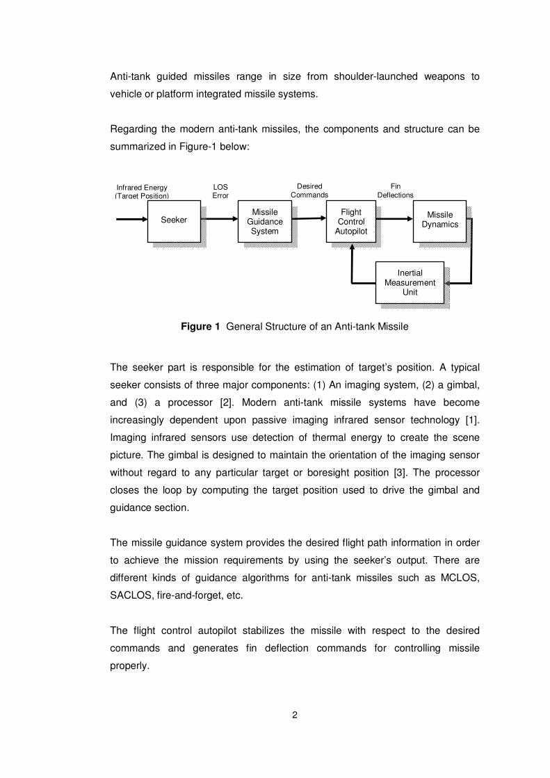
Regarding the modern anti-tank missiles, the components and structure can be
summarized in Figure-1 below:
Figure 1 General Structure of an Anti-tank Missile
The seeker part is responsible for the estimation of target’s position. A typical
seeker consists of three major components: (1) An imaging system, (2) a gimbal,
and (3) a processor [2]. Modern anti-tank missile systems have become
increasingly dependent upon passive imaging infrared sensor technology [1].
Imaging infrared sensors use detection of thermal energy to create the scene
picture. The gimbal is designed to maintain the orientation of the imaging sensor
without regard to any particular target or boresight position [3]. The processor
closes the loop by computing the target position used to drive the gimbal and
guidance section.
The missile guidance system provides the desired flight path information in order
to achieve the mission requirements by using the seeker’s output. There are
different kinds of guidance algorithms for anti-tank missiles such as MCLOS,
SACLOS, fire-and-forget, etc.
The flight control autopilot stabilizes the missile with respect to the desired
commands and generates fin deflection commands for controlling missile
properly.
Flight Control
Autopilot
Fin Deflections
Missile Dynamics
Inertial Measurement
Unit
Missile Guidance System
Desired Commands
Seeker
LOS Error
Infrared Energy (Target Position)
3
When designing the flight control autopilot, knowledge of the missile dynamics
and airframe are critical. Generic missiles are composed of 12 nonlinear
equations.
1.2 Scope of the Thesis
The thesis is organized in the following manner:
In Chapter 2, the mathematical model of the missile is constructed. It models the
aerodynamic forces and moments acting on the missile. These come up to be 12
nonlinear equations (6 kinematics and 6 dynamics). These equations are primarily
functions of aerodynamic coefficients. They are found using Missile DATCOM
software. Nonlinear equations are linearized in order to represent them in state-
space.
In Chapter 3, two different flight control autopilot designs are studied. They are
based on PID (proportional integral derivative) and LQR (linear quadratic
regulator) techniques. Their performances are compared according to the
simulation results.
In Chapter 4, an imaging infrared seeker model is given. Seeker subcomponents
are presented one by one. The gimbal structure is modeled and target detection
and tracking schemes are applied. Centroid, correlation and active contour
(snake) tracking algorithms are presented in detail and proposed tracking
algorithm, which combines positive sides of these methods, is developed.
Guidance design is presented for providing the proper flight path according to the
target state.
In Chapter 5, different simulations related with target contrast, clutter, noise, field-
of-view and countermeasures are discussed. Advantages of proposed algorithm
instead of using centroid, correlation and active contour methods alone are
presented.
In Chapter 6, overall study is concluded and recommendations for future works
are presented.
4
CHAPTER 2
2 MATHEMATICAL MODEL OF A GENERIC MISSILE
During the design of the flight control autopilot, missile mathematical modeling is
one of the most important stages. In this chapter, missile mathematical model will
be constructed using 12 nonlinear equations (6 kinematics and 6 dynamics) for a
6 DOF (degree-of-freedom) representation. Kinematics equations are the
consequences of transformation matrix applications that relates the reference axis
systems through the Euler Angles and dynamic equations are derived by
Newton’s second law of motion, which relates the summation of the external
forces and moments to the linear and angular accelerations of the body [5]. Since
several coordinate systems are used, frame definitions of missile will be
described. Finally, linearization of 12 nonlinear equations based on several
assumptions will be presented.
2.1 Frame Definitions
Two coordinate frames can be defined in order to describe the motion of the
missile: Normal Earth-fixed frame FE and Body frame FB. Both of them are three-
dimensional, orthogonal and right-handed [6].
2.1.1 Normal Earth-Fixed Frame
The origin of the frame is linked to a fixed point O on the Earth and its axes are
xE,yE,zE. The x-axis is directed towards the geographical North, the z-axis is

5
directed towards the descending direction of gravitational attraction and the y-axis
is the complementing axis.
Figure 2 Normal Earth-Fixed Coordinate System
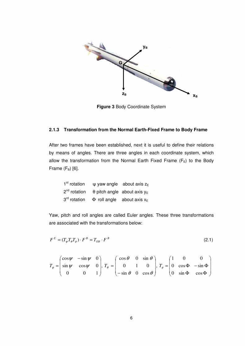
2.1.2 Body Frame
The origin of the body frame is linked to the missile body and the center of mass.
Its axes are xB,yB,zB. The x-axis, called the roll axis, points towards the front
belonging the symmetrical plane; the y-axis, called the pitch axis, is directed
towards the lateral side of the missile; and the z-axis, called the yaw axis, is the
complementing axis. G point is the center of mass.
zE
xE O
6
Figure 3 Body Coordinate System
2.1.3 Transformation from the Normal Earth-Fixed Frame to Body Frame
After two frames have been established, next it is useful to define their relations
by means of angles. There are three angles in each coordinate system, which
allow the transformation from the Normal Earth Fixed Frame (FE) to the Body
Frame (FB) [6].
1st rotation ψ yaw angle about axis zE
2nd rotation θ pitch angle about axis yE
3rd rotation Φ roll angle about axis xE
Yaw, pitch and roll angles are called Euler angles. These three transformations
are associated with the transformations below:
B
EB
BE FTFTTTF ⋅=⋅= )( φθψ (2.1)
−
=
100
0cossin
0sincos
ψψ
ψψ
ϕT ,
−
=
θθ
θθ
θ
cos0sin
010
sin0cos
T ,
ΦΦ
Φ−Φ=
cossin0
sincos0
001
φT
xB zB
yB
G
7
ΦΦ−
Φ−ΦΦ+Φ
Φ+ΦΦ−Φ
=
ΦΦ
Φ−Φ⋅
−
⋅
−
=
coscossincossin
cossinsincossincoscossinsinsincossin
sinsincossincoscossincossinsincoscos
cossin0
sincos0
001
cos0sin
010
sin0cos
100
0cossin
0sincos
θθθ
ψψθψψθθψ
ψθψψψθψθ
θθ
θθ
ψψ
ψψ
EBT
(2.2)
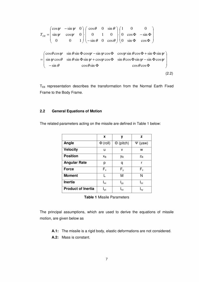
TEB representation describes the transformation from the Normal Earth Fixed
Frame to the Body Frame.
2.2 General Equations of Motion
The related parameters acting on the missile are defined in Table 1 below:
x y z
Angle Φ (roll) Θ (pitch) Ψ (yaw)
Velocity u v w
Position xB yB zB
Angular Rate p q r
Force Fx Fy Fz
Moment L M N
Inertia Ixx Iyy Izz
Product of Inertia Iyz Ixz Ixy
Table 1 Missile Parameters
The principal assumptions, which are used to derive the equations of missile
motion, are given below as
A.1: The missile is a rigid body, elastic deformations are not considered.
A.2: Mass is constant.
8
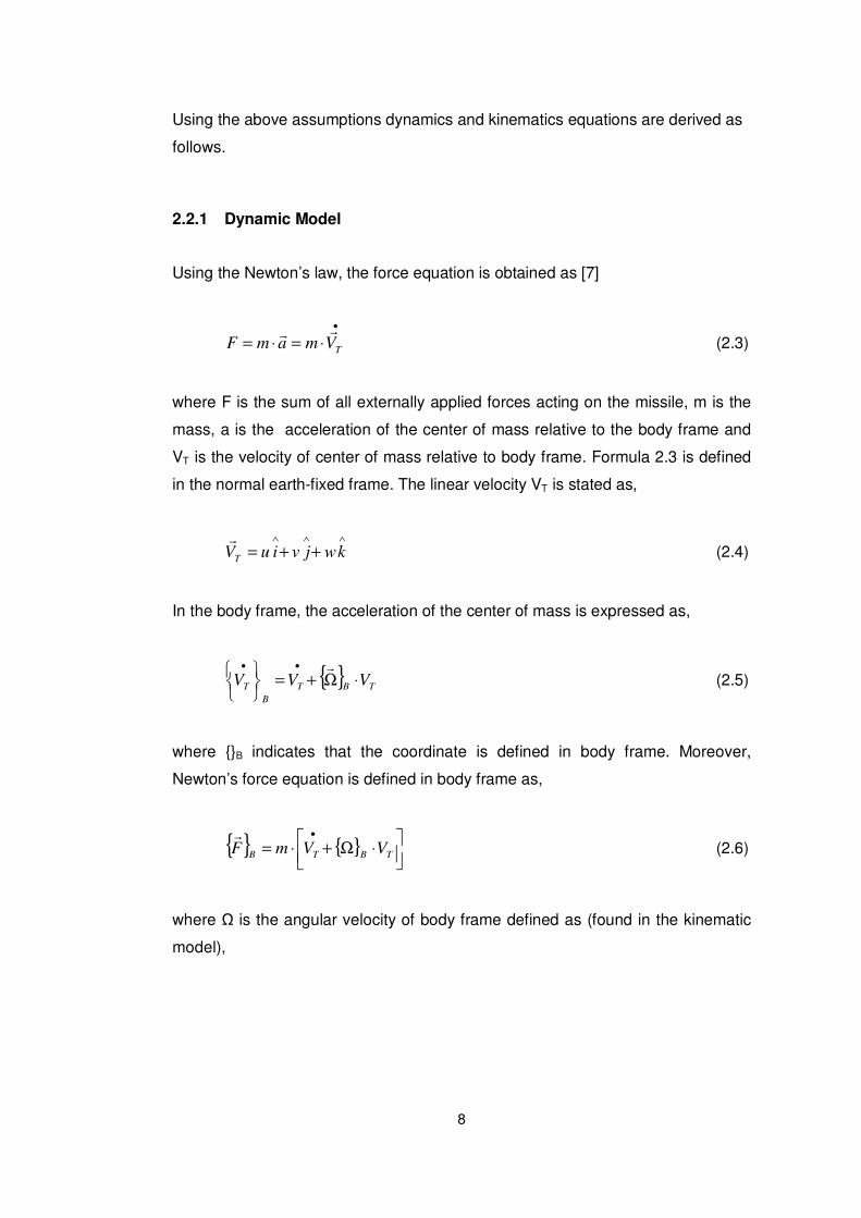
Using the above assumptions dynamics and kinematics equations are derived as
follows.
2.2.1 Dynamic Model
Using the Newton’s law, the force equation is obtained as [7]
•
⋅=⋅=T
VmamFrr
(2.3)
where F is the sum of all externally applied forces acting on the missile, m is the
mass, a is the acceleration of the center of mass relative to the body frame and
VT is the velocity of center of mass relative to body frame. Formula 2.3 is defined
in the normal earth-fixed frame. The linear velocity VT is stated as,
∧∧∧
++= kwjviuVT
r (2.4)
In the body frame, the acceleration of the center of mass is expressed as,
TBT
B
T VVV ⋅Ω+=
•• r
(2.5)
where B indicates that the coordinate is defined in body frame. Moreover,
Newton’s force equation is defined in body frame as,
⋅Ω+⋅=
•
TBTB VVmFr
(2.6)
where Ω is the angular velocity of body frame defined as (found in the kinematic
model),
9
−
−
−
=Ω
0
0
0
pq
pr
qr
B
r (2.7)
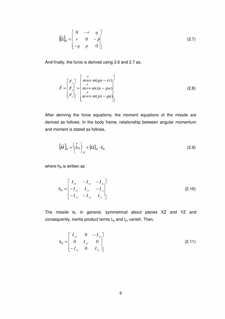
And finally, the force is derived using 2.6 and 2.7 as,
−+
−+
−+
=
=•
•
•
)(
)(
)(
qupvmwm
pwrumvm
rvqwmum
F
F
F
F
z
y
xr
(2.8)
After deriving the force equations, the moment equations of the missile are
derived as follows. In the body frame, relationship between angular momentum
and moment is stated as follows,
BB
B
BB hhM ⋅Ω+
=•r
(2.9)
where hB is written as
−−
−−
−−
=
zzyzxz
yzyyxy
xzxyxx
B
III
III
III
h (2.10)
The missile is, in general, symmetrical about planes XZ and YZ and
consequently, inertia product terms Ixy and Iyz vanish. Then,
−
−
=
zzxz
yy
xzxx
B
II
I
II
h
0
00
0
(2.11)

10
Ixx, Iyy, Izz and Ixz are the mass moment of inertia and the product of inertia of the
missile about body-fixed coordinate frame. Thus, the moment equation is stated
as follows,
−
−
⋅
−
−
−
+
−
−
=
=••
•
••
zzxz
yy
xzxx
xzzz
yy
xzxx
II
I
II
pq
pr
qr
pIrI
qI
rIpI
N
M
L
M
0
00
0
0
0
0r
+−+−
−+−+
−−+−
=••
•
••
qrIpqIIpIrI
rpIprIIqI
pqIqrIIrIpI
xzxxyyxzzz
xzzzxxyy
xzyyzzxzxx
)(
)()(
)(
22 (2.12)
where L is defined as the roll moment, M is the pitch moment and N is the yaw
moment of missile.
2.2.2 Kinematic Model
The nonlinear equations of kinematics, describing the missile, can be divided into
two parts: one is governing the translational motion and the other one governing
the rotational motion. In the body frame, the kinematic equations can be
formulated as described next.
Using equation 2.2, the transformation matrix from the normal earth fixed frame to
body fixed frame relates the translational kinematic equations as
=
•
•
•
z
y
x
⋅
ΦΦ−
Φ−ΦΦ+Φ
Φ+ΦΦ−Φ
w
v
u
coscossincossin
cossinsincossincoscossinsinsincossin
sinsincossincoscossincossinsincoscos
θθθ
ψψθψψθθψ
ψθψψψθψθ
(2.13)

11
Secondly, The Euler rates with respect to the body fixed frame construct the
rotational kinematic equations as follows:
( )T
EBEB TTIIdentity ×== (2.14)
Taking the derivative of equation 2.14 leads
( ) ( )( ) 0=×=T
EBEBTT
dt
dI
dt
d (2.15)
( ) ( ) ( ) 0=⋅+⋅T
EBEB
T
EBEBT
dt
dTTT
dt
d (2.16)
( ) ( ) ( )T
EB
T
EB
T
EBEB Tdt
dTTT
dt
d
⋅−=⋅ (2.17)
Definition 2.1 (Skew-Symmetric of a Matrix) [7]
A matrix S is said to be skew-symmetric if:
TSS −= (2.18)
This implies that the off-diagonal matrix elements of S satisfy sij = -sji for i ≠ j while
the matrix diagonal consists of zero elements.
Using the definition 2.1, ( ) ( )T
EBEB TTdt
d⋅ is a skew-symmetric matrix and
consequently there exists a skew-symmetric matrix such that
( ) ( )
⋅
⋅=Ω
r
q
p
TTdt
d T
EBEB
~
(2.19)
Then, the skew-symmetric matrix is found as equation 2.7. Solving equation 2.19
and 2.7 leads following equation,
12
( )
)cos(
)sin()cos(
)sin()cos(
)cos()sin()tan(
θψ
θ
θ
Φ+Φ=
Φ−Φ=
Φ+Φ⋅+=Φ
•
•
•
qr
rq
rqp
(2.20)
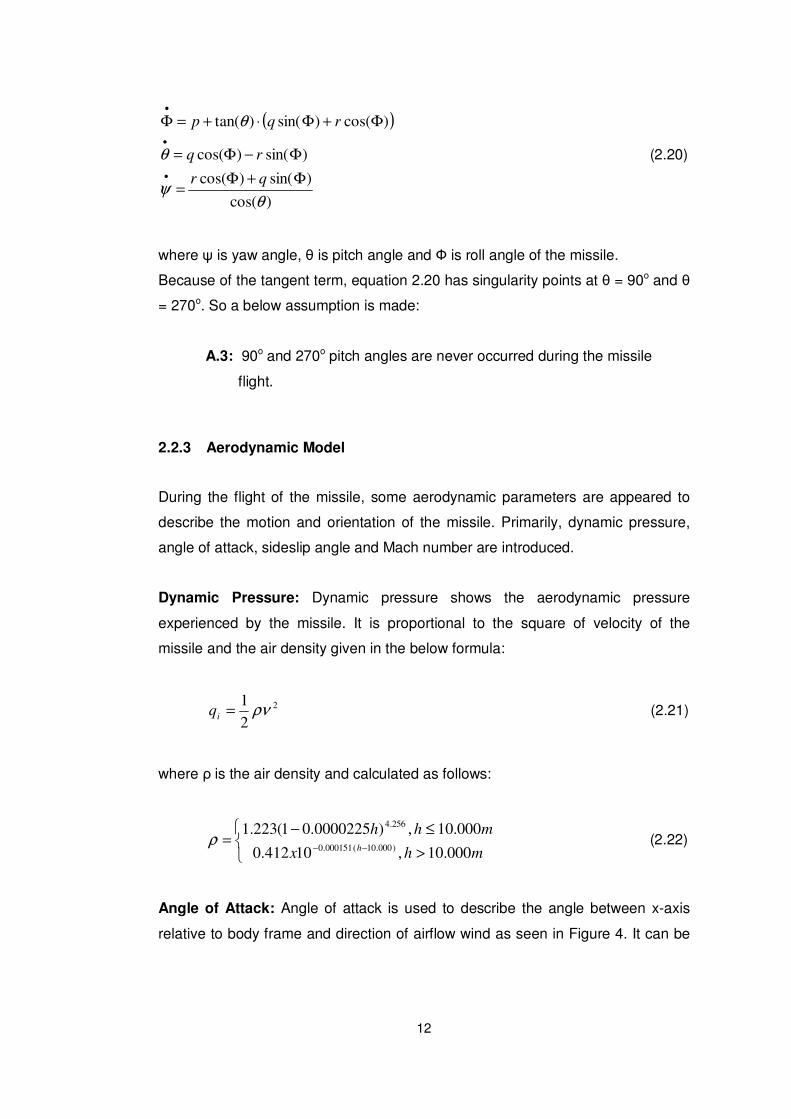
where ψ is yaw angle, θ is pitch angle and Ф is roll angle of the missile.
Because of the tangent term, equation 2.20 has singularity points at θ = 90o and θ
= 270o. So a below assumption is made:
A.3: 90o and 270o pitch angles are never occurred during the missile
flight.
2.2.3 Aerodynamic Model
During the flight of the missile, some aerodynamic parameters are appeared to
describe the motion and orientation of the missile. Primarily, dynamic pressure,
angle of attack, sideslip angle and Mach number are introduced.
Dynamic Pressure: Dynamic pressure shows the aerodynamic pressure
experienced by the missile. It is proportional to the square of velocity of the
missile and the air density given in the below formula:
2
2
1ρν=iq (2.21)
where ρ is the air density and calculated as follows:
>
≤−=
−− mhx
mhhh 000.10,10412.0
000.10,)0000225.01(223.1)000.10(000151.0
256.4
ρ (2.22)
Angle of Attack: Angle of attack is used to describe the angle between x-axis
relative to body frame and direction of airflow wind as seen in Figure 4. It can be

13
described as the angle between where the missile is pointing and where it is
going. It is defined as
=
u
warctanα (2.23)
Since w is much smaller than u, the above equation can be written as,
≅
u
wα (2.24)
Sideslip Angle: Sideslip angle relates to the displacement of the aircraft
centerline from the relative wind as seen in the Figure 4. It is defined as,
=
TV
varctanβ (2.25)
Since v is much smaller than VT (can be taken as u, so 0≅•
u ), the above equation
can be written as,
≅
≅
u
v
V
v
T
β (2.26)
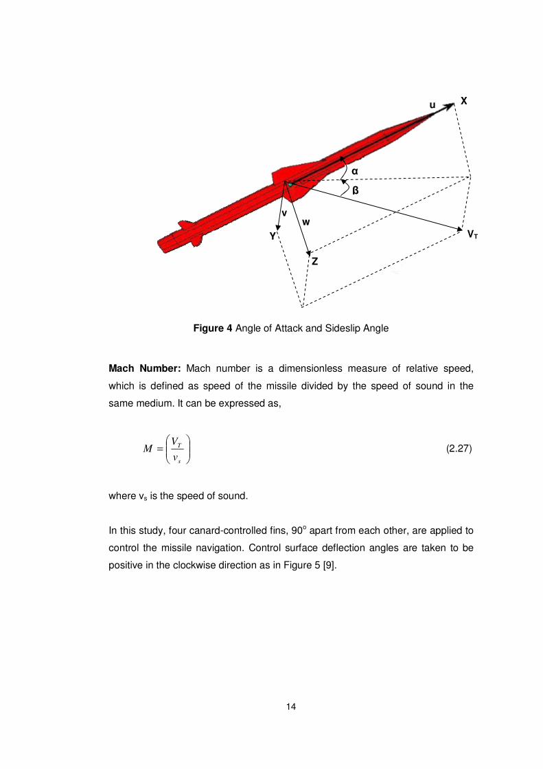
14
Figure 4 Angle of Attack and Sideslip Angle
Mach Number: Mach number is a dimensionless measure of relative speed,
which is defined as speed of the missile divided by the speed of sound in the
same medium. It can be expressed as,
=
s
T
v
VM (2.27)
where vs is the speed of sound.
In this study, four canard-controlled fins, 90o apart from each other, are applied to
control the missile navigation. Control surface deflection angles are taken to be
positive in the clockwise direction as in Figure 5 [9].
v
α
β
VT
u X
Z
Y
w
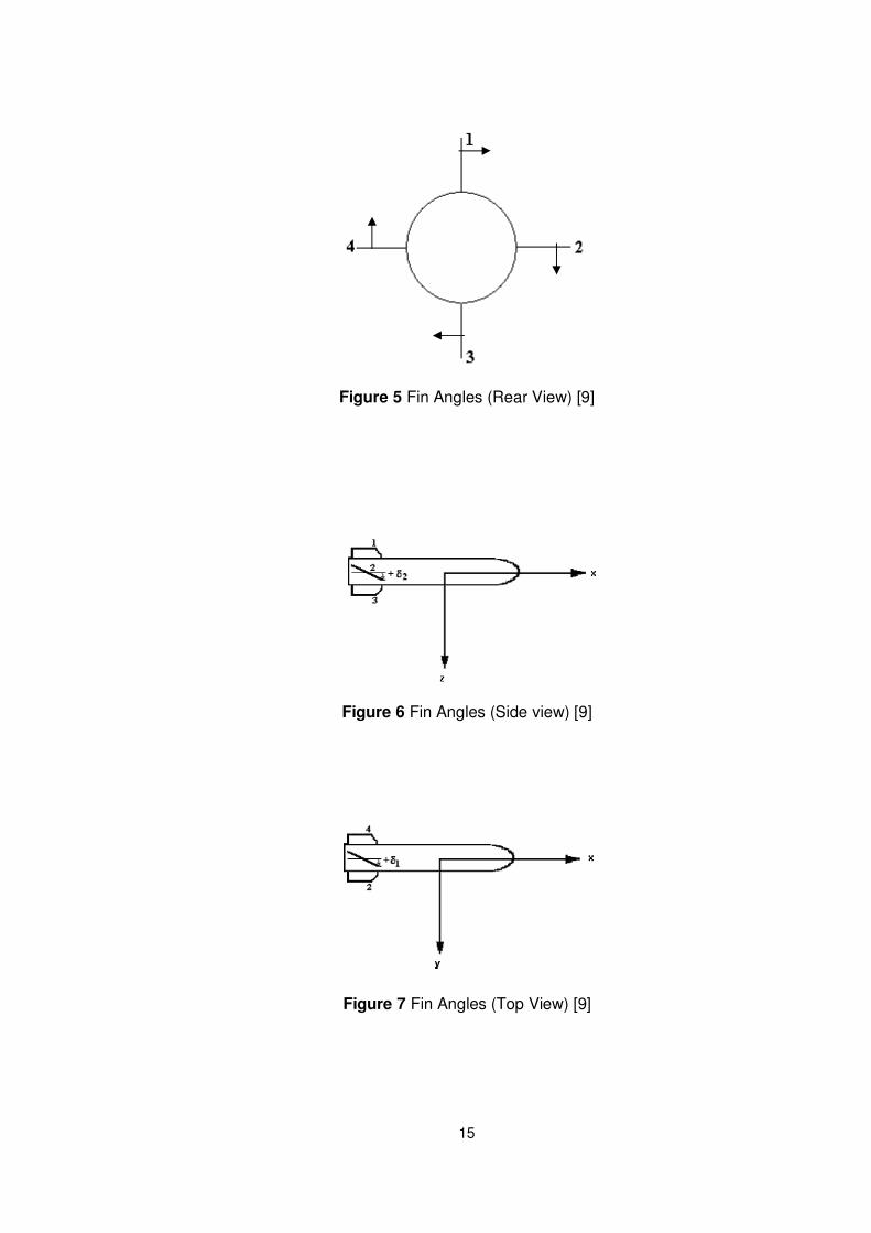
15
Figure 5 Fin Angles (Rear View) [9]
Figure 6 Fin Angles (Side view) [9]
Figure 7 Fin Angles (Top View) [9]
16
4321 ,,, δδδδ angles represent first, second, third and fourth control fin angles,
respectively. In the dynamical equations of motion, control surface deflections are
categorized in three planes, namely roll, pitch and yaw planes as
aδ : aileron fin deflections
eδ : elevator fin deflections
rδ : rudder fin deflections
These fin deflections are calculated using 4321 ,,, δδδδ as below:
4
4321 δδδδδ
+++=
a (2.28)
2
42 δδδ
−=
e (2.29)
2
31 δδδ
−=
r (2.30)
There exist three different forces acting on the missile: (1) Aerodynamic force (2)
Gravitational force (3) Propulsion force and two different type of moments acting
on the missile (1) Aerodynamic moment (2) Propulsion moment. Therefore, force
and moment equations can be separated as follows
Φ++
Φ++
−+
=
−+
−+
−+
=
=•
•
•
)cos()cos(
)sin()cos(
)sin(
)(
)(
)(
θ
θ
θ
mgPSCq
mgPSCq
mgPSCq
qupvmwm
pwrumvm
rvqwmum
F
F
F
F
zzi
yyi
xxi
z
y
x
(2.31)
where qi is the dynamic pressure; S is the cross-sectional area of the missile;
Cx,Cy,Cz are the force coefficients; Px,Py,Pz are the propulsion forces.

17
Further derivations lead following equations:
( )
( ) ( )
( ) ( )
Φ++
++−
Φ++
++−
−+
++−
=
•
•
•
coscos
sincos
sin
θ
θ
θ
gm
PSCqqupv
gm
PSCqpwru
gm
PSCqrvqw
w
v
u
zzi
yyi
xxi
(2.32)
Similarly, for the rotational dynamics, the following equations can be derived:
+
+
+
=
+−+−
−+−+
−−+−
=••
•
••
NMi
MMi
LMi
xzxxyyxzzz
xzzzxxyy
xzyyzzxzxx
SCdqN
SCdqM
SCdqL
qrIpqIIpIrI
rpIprIIqI
pqIqrIIrIpI
M
)(
)()(
)(
22 (2.33)
where qi is the dynamic pressure; S is the cross-sectional area of the missile; dM
is the missile diameter; CL,CM,CN are the moment coefficients.
Further derivations lead following equations:
+−−
−
+−−−
−
++−
−
=
•
•
•
•
•
zz
NMi
zz
xz
zz
xxyy
zz
xz
yy
MMi
yy
xz
yy
zzxx
xx
LMi
xx
xz
xx
yyzz
xx
xz
I
SCdqqr
I
Ipq
I
IIp
I
I
I
SCdqrp
I
Ipr
I
II
I
SCdqpq
I
Iqr
I
IIr
I
I
r
q
p
)(
)()(
)(
22 (2.34)
The aerodynamic coefficients (Ci) can be defined with respect to flight parameters
such as angle of attack, sideslip angle, Mach number, fin deflections and angular
rates [8]. These coefficients are nonlinear functions of flight parameters. There
exist some experimental methods like wind-tunnel tests or computational fluid
dynamics methods in order to calculate the aerodynamic coefficients, but
MISSILE DATCOM software will be used alternatively in this thesis. Details of this
software are given in Appendix A.

18
Aerodynamic coefficients can be defined as follows
XC : Axial force coefficient
YC : Side force coefficient
ZC : Normal force coefficient
LC : Rolling moment coefficient
MC : Pitching moment coefficient
NC : Yawing moment coefficient
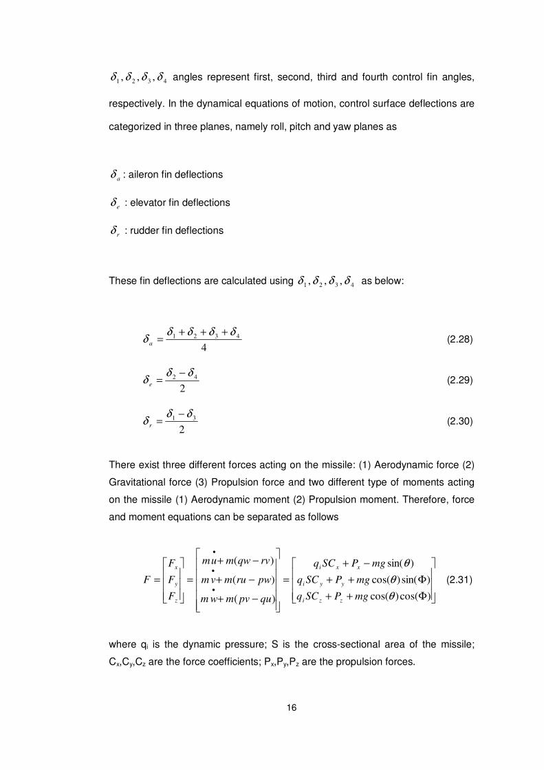
Axial, normal force coefficients and pitching moment coefficient will be given for
selected missile configuration in Figure 8 and 9.
Figure 8 Axial and Normal Force Coefficients
19
Figure 9 Pitching Moment Coefficient
The aerodynamic coefficients will be linearized by using the Taylor series
expansion around the trim points of the flight parameters in order to represent
them in flight autopilot design:
HOTV
drMC
V
dqMC
V
dpMCMCMC
MCMCMCMCC
T
Mir
T
Miq
T
Mipriei
aiiiii
re
a
+⋅
⋅⋅+⋅
⋅⋅
+⋅
⋅⋅+⋅+⋅
+⋅+⋅+⋅+=
2),(
2),(
2),(),(),(
),(),(),(),(0
αα
αδαδα
δαβαααα
δδ
δβα
(2.35)
where HOT stands for higher order terms and T
M
V
d
⋅2 term is included as a
multiplier to the aerodynamic derivatives to make them dimensionless [8].
Aerodynamic derivatives can be written as
0
),(
ii
i
i
i
i
CMC
θθ
θθ
α=
∂
∂= (2.36)

20
The aerodynamic derivative values are taken at the trim values of the flight
parameters and they are kept only as a non-linear function of mach number and
angle-of-attack. Since along the flight path of the missile, parameters will be
small, so the trim points can be taken as zero. After linearization, the
dimensionless aerodynamic coefficients can be written as follows
T
M
nrrnnn
T
M
mqemmm
T
Mlpall
T
M
zqezzz
T
M
yrryyy
xx
V
drMCMCMCC
V
dqMCMCMCC
V
dpMCMCC
V
dqMCMCMCC
V
drMCMCMCC
MCC
⋅⋅⋅+⋅+⋅=
⋅⋅⋅+⋅+⋅=
⋅⋅⋅+⋅=
⋅⋅⋅+⋅+⋅=
⋅⋅⋅+⋅+⋅=
=
2),(),(),(
2),(),(),(
2),(),(
2),(),(),(
2),(),(),(
),(0
αδαβα
αδααα
αδα
αδααα
αδαβα
α
δβ
δα
δ
δα
δβ
(2.37)
Because of the missile symmetry, aerodynamic coefficients can be taken as
follows:
nrmq
nm
nm
yrzq
yz
yz
CC
CC
CC
CC
CC
CC
=
−=
−=
−=
=
=
δδ
βα
δδ
βα
(2.38)
2.2.4 Linearization of Equations
There are several ways to linearize the equations of missile motion. One of them
is the specification of flight conditions. By applying the following assumptions,
dynamic and kinematic equations of motion can be linearized.
21
A.4: The velocity of missile, ambient temperature and ambient density are
constant.
A.5: Angle of attack, side-slip angle and fin deflections are constant.
A.6: Rolling motion is very small ( 0≅p )
A.7: Components of gravitational acceleration are external disturbances.
A.8: The flight after the boost phase is considered so the propulsion forces
(Px,Py,Pz) and moments (L,M,N) are not included in the equations.
A.9: Coordinate system is located at the center of gravity and XZ plane is
axis-symmetric, so that the mass distribution is such that Ixz = Iyz = Ixy = 0 and
Iyy = Izz.
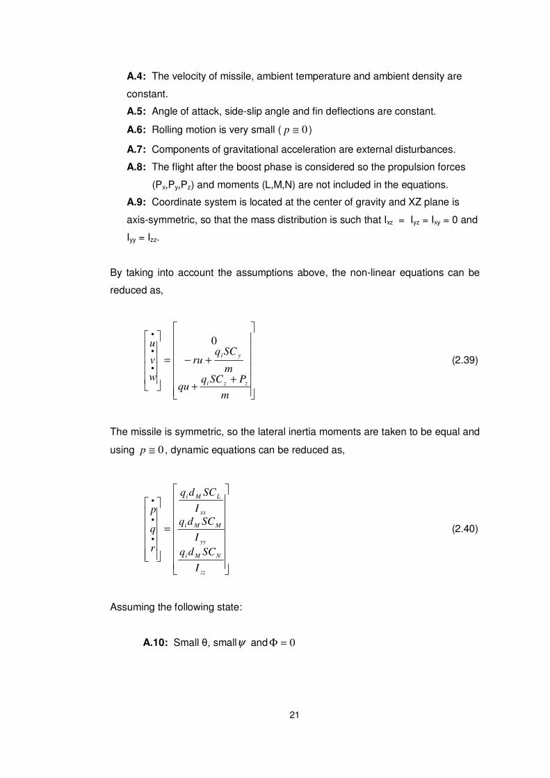
By taking into account the assumptions above, the non-linear equations can be
reduced as,
++
+−=
•
•
•
m
PSCqqu
m
SCqru
w
v
u
zzi
yi
0
(2.39)
The missile is symmetric, so the lateral inertia moments are taken to be equal and
using 0≅p , dynamic equations can be reduced as,
=
•
•
•
zz
NMi
yy
MMi
xx
LMi
I
SCdq
I
SCdq
I
SCdq
r
q
p
(2.40)
Assuming the following state:
A.10: Small θ, smallψ and 0=Φ
22
leads
( ) ( )( ) ( )( ) ( ) 1cos,sin
1cos,sin
1cos,0sin
≅≅
≅≅
=Φ=Φ
ψψψ
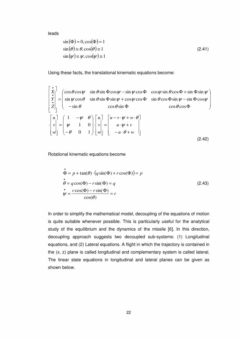
θθθ (2.41)
Using these facts, the translational kinematic equations become:
+⋅−
+⋅
⋅+⋅−
=
⋅
−
−
=
⋅
ΦΦ−
Φ−ΦΦ+Φ
Φ+ΦΦ−Φ
=
•
•
•
wu
vu
wvu
w
v
u
w
v
u
Z
Y
X
θ
ψ
θψ
θ
ψ
θψ
θθθ
ψψθψψθθψ
ψθψψψθψθ
10
01
1
coscossincossin
cossinsincossincoscossinsinsincossin
sinsincossincoscossincossinsincoscos
(2.42)
Rotational kinematic equations become
( )
rrr
qrq
prqp
=Φ−Φ
=
=Φ−Φ=
=Φ+Φ⋅+=Φ
•
•
•
)cos(
)sin()cos(
)sin()cos(
)cos()sin()tan(
θψ
θ
θ
(2.43)
In order to simplify the mathematical model, decoupling of the equations of motion
is quite suitable whenever possible. This is particularly useful for the analytical
study of the equilibrium and the dynamics of the missile [6]. In this direction,
decoupling approach suggests two decoupled sub-systems: (1) Longitudinal
equations, and (2) Lateral equations. A flight in which the trajectory is contained in
the (x, z) plane is called longitudinal and complementary system is called lateral.
The linear state equations in longitudinal and lateral planes can be given as
shown below.
23
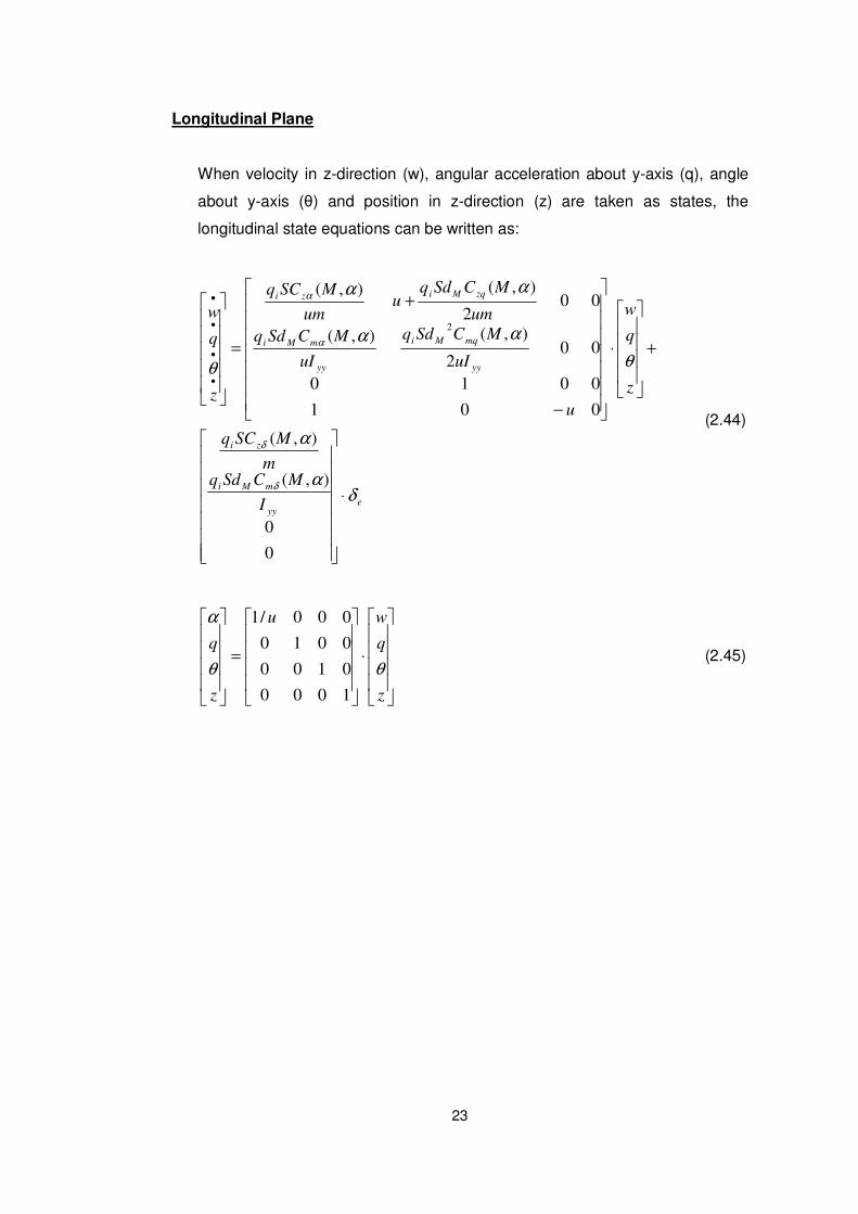
Longitudinal Plane
When velocity in z-direction (w), angular acceleration about y-axis (q), angle
about y-axis (θ) and position in z-direction (z) are taken as states, the
longitudinal state equations can be written as:
eyy
mMi
zi
yy
mqMi
yy
mMi
zqMizi
I
MCSdqm
MSCq
z
q
w
u
uI
MCSdq
uI
MCSdq
um
MCSdqu
um
MSCq
z
q
w
δα
α
θ
αα
αα
θ
δ
δ
α
α
⋅
+
⋅
−
+
=
•
•
•
•
0
0
),(
),(
001
0010
002
),(),(
002
),(),(
2
(2.44)
⋅
=
z
q
wu
z
q
θθ
α
1000
0100
0010
000/1
(2.45)
24
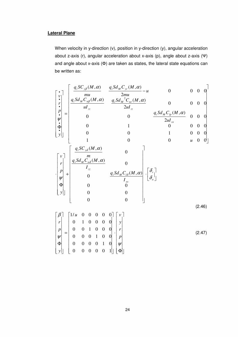
Lateral Plane
When velocity in y-direction (v), position in y-direction (y), angular acceleration
about z-axis (r), angular acceleration about x-axis (p), angle about z-axis (Ψ)
and angle about x-axis (Φ) are taken as states, the lateral state equations can
be written as:
⋅
+
Φ
⋅
−
=
Φ•
•
•
•
•
•
a
r
xx
lMi
zz
nMi
yi
xx
lpMi
zz
nrMi
zz
nMi
yrMiyi
I
MCSdq
I
MCSdqm
MSCq
y
p
r
v
u
uI
MCSdq
uI
MCSdq
uI
MCSdq
umu
MCSdq
mu
MSCq
y
p
r
v
δ
δα
α
α
ψ
α
αα
αα
ψ
δ
δ
δ
β
β
00
00
00
),(0
0),(
0),(
00001
000100
000010
0002
),(00
00002
),(),(
00002
),(),(
2
(2.46)
Φ
⋅
=
Φ ψ
ψ
β
p
r
y
vu
y
p
r
100000
010000
001000
000100
000010
00000/1
(2.47)
25
CHAPTER 3
3 FLIGHT CONTROL AUTOPILOT
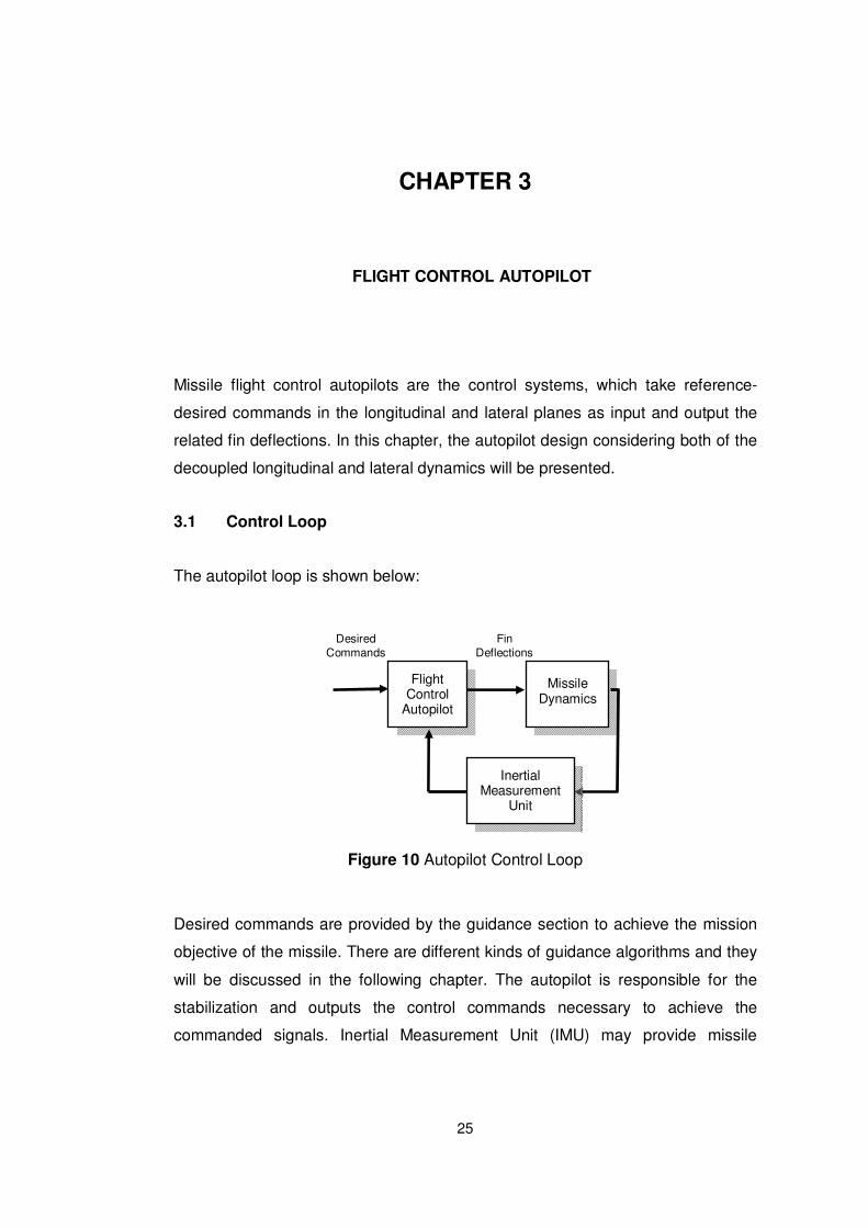
Missile flight control autopilots are the control systems, which take reference-
desired commands in the longitudinal and lateral planes as input and output the
related fin deflections. In this chapter, the autopilot design considering both of the
decoupled longitudinal and lateral dynamics will be presented.
3.1 Control Loop
The autopilot loop is shown below:
Figure 10 Autopilot Control Loop
Desired commands are provided by the guidance section to achieve the mission
objective of the missile. There are different kinds of guidance algorithms and they
will be discussed in the following chapter. The autopilot is responsible for the
stabilization and outputs the control commands necessary to achieve the
commanded signals. Inertial Measurement Unit (IMU) may provide missile
Flight Control
Autopilot
Fin Deflections
Missile Dynamics
Inertial Measurement
Unit
Desired Commands

26
position, acceleration or rate parameters and they are compared with the
predefined trajectories in autopilot section. Not every parameter is measurable,
but acceleration and rate can be measured with a three-axes accelerometer and
three-axes gyroscope, respectively. The autopilot closes the loop in this scheme
to achieve the required performance criteria.
3.2 Design Requirements
Every design should be based on some requirements, which are related to the
performance of the overall system. Following are the design requirements for the
autopilot system.
• Rise time should be less than 0.5 seconds,
• Percentage overshot for the step input should be less than 30%,
• Settling time should be less than 1.5 seconds,
• Steady-state error should be less than 5%.
3.3 PID Autopilot Design
While a variety of control methods can be formulated for the autopilot controls,
basic PID (proportional-integral-derivative) controller will be implemented in this
section. PID controllers are widely used in aerospace applications and they simply
attempt to correct the error between measured sensor parameters and the
desired values by calculating and outputting a corrective action that can adjust the
process accordingly. PID controller has the transfer function:
sKs
KKsG
D
I
PC⋅++=)( (3.1)
The controller provides a proportional term, an integral term, and a derivative term
[11]. The equation for the output in the time-domain is
( ) ( ) ( ) ( )∫ ++=
dt
tdeKdtteKteKtu
DIP (3.2)
27
where KP is the “proportional gain”, KI is the “integral gain” and KD is the
“derivative gain”.
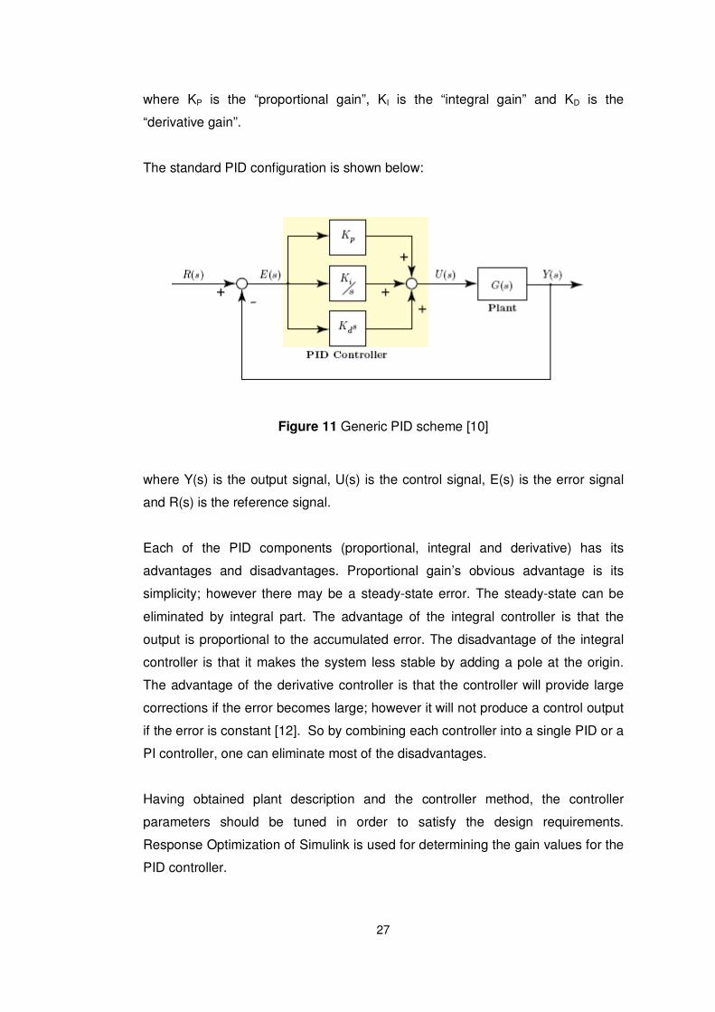
The standard PID configuration is shown below:
Figure 11 Generic PID scheme [10]
where Y(s) is the output signal, U(s) is the control signal, E(s) is the error signal
and R(s) is the reference signal.
Each of the PID components (proportional, integral and derivative) has its
advantages and disadvantages. Proportional gain’s obvious advantage is its
simplicity; however there may be a steady-state error. The steady-state can be
eliminated by integral part. The advantage of the integral controller is that the
output is proportional to the accumulated error. The disadvantage of the integral
controller is that it makes the system less stable by adding a pole at the origin.
The advantage of the derivative controller is that the controller will provide large
corrections if the error becomes large; however it will not produce a control output
if the error is constant [12]. So by combining each controller into a single PID or a
PI controller, one can eliminate most of the disadvantages.
Having obtained plant description and the controller method, the controller
parameters should be tuned in order to satisfy the design requirements.
Response Optimization of Simulink is used for determining the gain values for the
PID controller.
28
3.3.1 Longitudinal PID Control
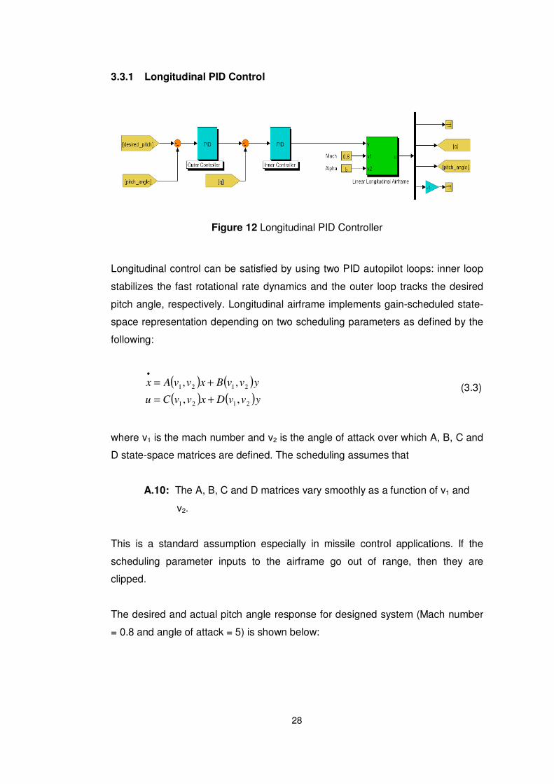
Figure 12 Longitudinal PID Controller
Longitudinal control can be satisfied by using two PID autopilot loops: inner loop
stabilizes the fast rotational rate dynamics and the outer loop tracks the desired
pitch angle, respectively. Longitudinal airframe implements gain-scheduled state-
space representation depending on two scheduling parameters as defined by the
following:
( ) ( )( ) ( )yvvDxvvCu
yvvBxvvAx
2121
2121
,,
,,
+=
+=•
(3.3)
where v1 is the mach number and v2 is the angle of attack over which A, B, C and
D state-space matrices are defined. The scheduling assumes that
A.10: The A, B, C and D matrices vary smoothly as a function of v1 and
v2.
This is a standard assumption especially in missile control applications. If the
scheduling parameter inputs to the airframe go out of range, then they are
clipped.
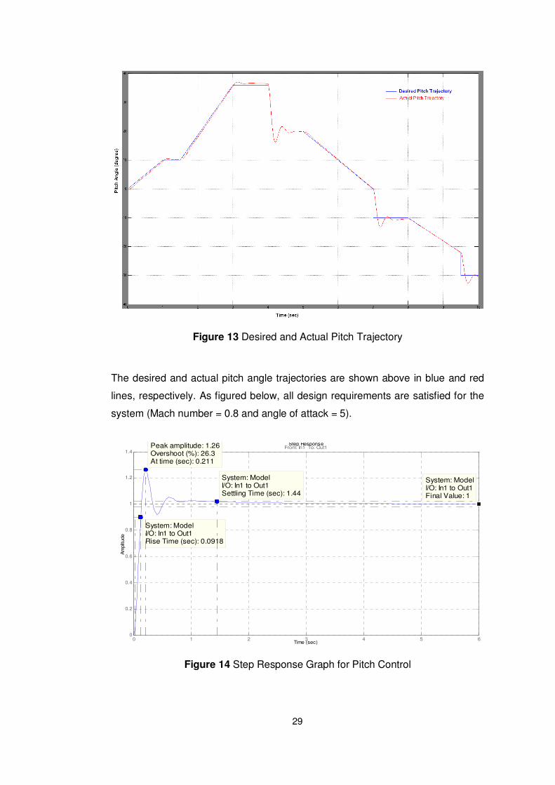
The desired and actual pitch angle response for designed system (Mach number
= 0.8 and angle of attack = 5) is shown below:
29
Figure 13 Desired and Actual Pitch Trajectory
The desired and actual pitch angle trajectories are shown above in blue and red
lines, respectively. As figured below, all design requirements are satisfied for the
system (Mach number = 0.8 and angle of attack = 5).
Step Response
Time (sec)
Am
plitu
de
0 1 2 3 4 5 60
0.2
0.4
0.6
0.8
1
1.2
1.4Peak amplitude: 1.26Overshoot (%): 26.3At time (sec): 0.211
System: ModelI/O: In1 to Out1Rise Time (sec): 0.0918
System: ModelI/O: In1 to Out1Settling Time (sec): 1.44
System: ModelI/O: In1 to Out1Final Value: 1
From: In1 To: Out1
Figure 14 Step Response Graph for Pitch Control
30
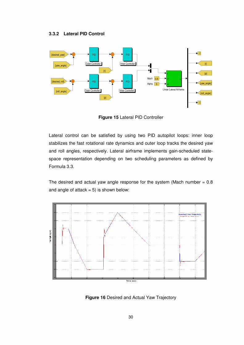
3.3.2 Lateral PID Control
Mach
Linear Lateral Airframe
Inner Controller
Inner Controller
Outer Controller
Outer Controller
AlphaPID
PID
PID
PID
[p]
[roll_angle]
[yaw_angle]
[r][yaw_angle]
[desired_yaw]
[roll_angle]
[desired_roll]
[p]
[r]
0.8
5
y
v1
v2
u
Figure 15 Lateral PID Controller
Lateral control can be satisfied by using two PID autopilot loops: inner loop
stabilizes the fast rotational rate dynamics and outer loop tracks the desired yaw
and roll angles, respectively. Lateral airframe implements gain-scheduled state-
space representation depending on two scheduling parameters as defined by
Formula 3.3.
The desired and actual yaw angle response for the system (Mach number = 0.8
and angle of attack = 5) is shown below:
Figure 16 Desired and Actual Yaw Trajectory
31
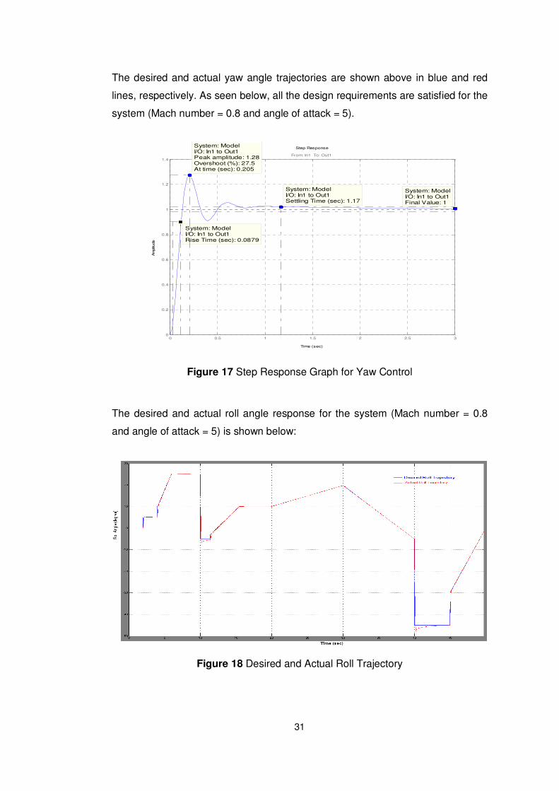
The desired and actual yaw angle trajectories are shown above in blue and red
lines, respectively. As seen below, all the design requirements are satisfied for the
system (Mach number = 0.8 and angle of attack = 5).
Step Response
Time (sec)
Am
plitude
0 0.5 1 1.5 2 2.5 30
0.2
0.4
0.6
0.8
1
1.2
1.4
System: ModelI/O: In1 to Out1Peak amplitude: 1.28Overshoot (%): 27.5At time (sec): 0.205
System: ModelI/O: In1 to Out1Settling Time (sec): 1.17
System: ModelI/O: In1 to Out1Final Value: 1
System: ModelI/O: In1 to Out1Rise Time (sec): 0.0879
From: In1 To: Out1
Figure 17 Step Response Graph for Yaw Control
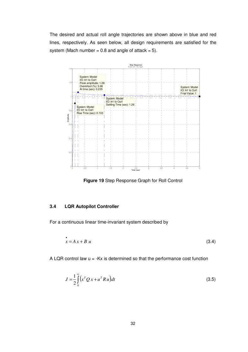
The desired and actual roll angle response for the system (Mach number = 0.8
and angle of attack = 5) is shown below:
Figure 18 Desired and Actual Roll Trajectory
32
The desired and actual roll angle trajectories are shown above in blue and red
lines, respectively. As seen below, all design requirements are satisfied for the
system (Mach number = 0.8 and angle of attack = 5).
Step Response
Time (sec)
Am
plitu
de
0 0.5 1 1.5 2 2.5 3 3.5 4 4.5 50
0.2
0.4
0.6
0.8
1
1.2
1.4
System: ModelI/O: In1 to Out1Peak amplitude: 1.06Overshoot (%): 5.96At time (sec): 0.235
System: ModelI/O: In1 to Out1Settling Time (sec): 1.26
System: ModelI/O: In1 to Out1Rise Time (sec): 0.103
System: ModelI/O: In1 to Out1Final Value: 1
From: In1 To: Out1
Figure 19 Step Response Graph for Roll Control
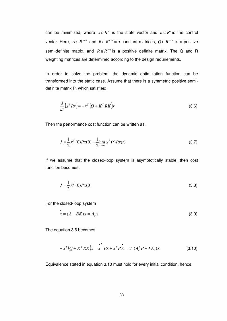
3.4 LQR Autopilot Controller
For a continuous linear time-invariant system described by
uBxAx +=•
(3.4)
A LQR control law u = -Kx is determined so that the performance cost function
( )∫∞
+=0
2
1dtuRuxQxJ
TT (3.5)
33
can be minimized, where nRx ∈ is the state vector and rRu ∈ is the control
vector. Here, nnRA ×∈ and rnRB ×∈ are constant matrices, nnRQ ×∈ is a positive
semi-definite matrix, and rrRR ×∈ is a positive definite matrix. The Q and R
weighting matrices are determined according to the design requirements.
In order to solve the problem, the dynamic optimization function can be
transformed into the static case. Assume that there is a symmetric positive semi-
definite matrix P, which satisfies:
( ) ( )xRKKQxPxxdt
d TTT +−= (3.6)
Then the performance cost function can be written as,
)()(lim2
1)0()0(
2
1tPxtxPxxJ T
t
T
∞→−= (3.7)
If we assume that the closed-loop system is asymptotically stable, then cost
function becomes:
)0()0(2
1PxxJ T= (3.8)
For the closed-loop system
xAxBKAxc
=−=•
)( (3.9)
The equation 3.6 becomes
( ) xPAPAxxPxPxxxRKKQx c
T
c
TT
T
TT)( +=+=+−
••
(3.10)
Equivalence stated in equation 3.10 must hold for every initial condition, hence
34
0=+++= QRKKPAPAg T
c
T
c (3.11)
Thus, the optimization problem is transformed into finding the feedback gains K
that minimizes the cost function J. The Lagrange multiplier approach is used to
solve the resultant constrained optimization problem. The Lagrangian is
gSPxxH T += )0()0(2
1 (3.12)
where S is a symmetric matrix of Lagrange multipliers. The necessary conditions
are:
BPSRKSK
H
xSASAP
H
QRKKPAPAgS
H
T
cc
T
c
T
c
−=∂
∂=
++=∂
∂=
+++==∂
∂=
2
10
)0(0
0
(3.13)
If R is positive definite, then the feedback gains (K) can be found as
PBRKT1−= (3.14)
So, there is no need to solve the S in order to find feedback gains. This result
leads us:
PBPBRQPAPA TT 10 −−++= (3.15)
which is called “Algebraic Riccati Equation”. Solving equation 3.15 is sufficient
to compute feedback gains. During the programming phase, MATLAB’s “lqr”
function is used to solve Riccati equations.
35
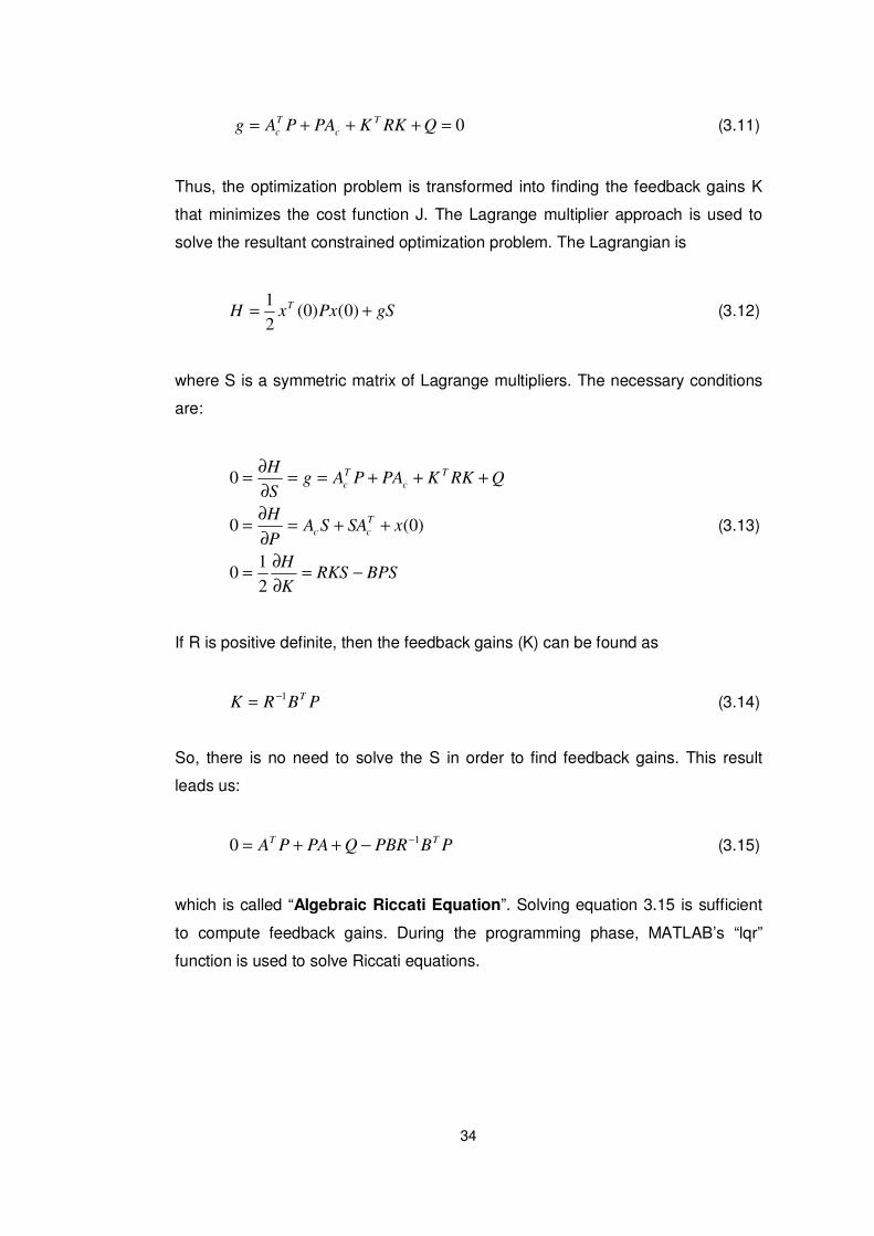
3.4.1 Longitudinal LQR Control
Velocity
Alpha
Linear Longitudinal Airframe1
y
v1
v2
u
K4-K-
K3-K-
K2-K-
K1-K-Integrator
1s
[z]
[alpha]
[q]
[pitch_angle]
Gain 1
-K-
[z]
[pitch_angle]
[q]
[alpha][pitch_angle]
[desired_pitch]
0.8
5
Figure 20 Longitudinal LQR Controller
Longitudinal motion can be controlled using an LQR controller, as well. The
feedback gains are found from MATLAB’s “lqr” function. Longitudinal airframe
implements gain-scheduled state-space representation depending on two
scheduling parameters as defined by Formula 3.3.
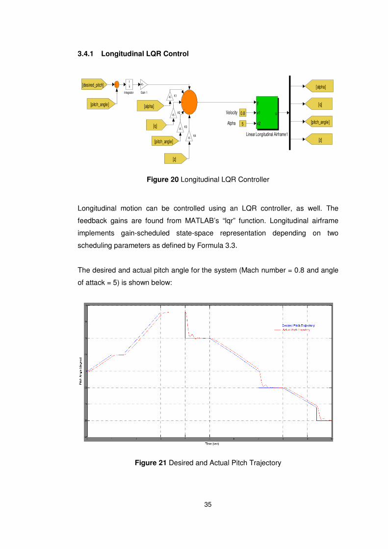
The desired and actual pitch angle for the system (Mach number = 0.8 and angle
of attack = 5) is shown below:
Figure 21 Desired and Actual Pitch Trajectory
36
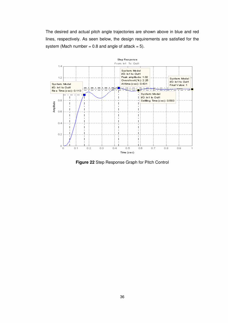
The desired and actual pitch angle trajectories are shown above in blue and red
lines, respectively. As seen below, the design requirements are satisfied for the
system (Mach number = 0.8 and angle of attack = 5).
Figure 22 Step Response Graph for Pitch Control
37
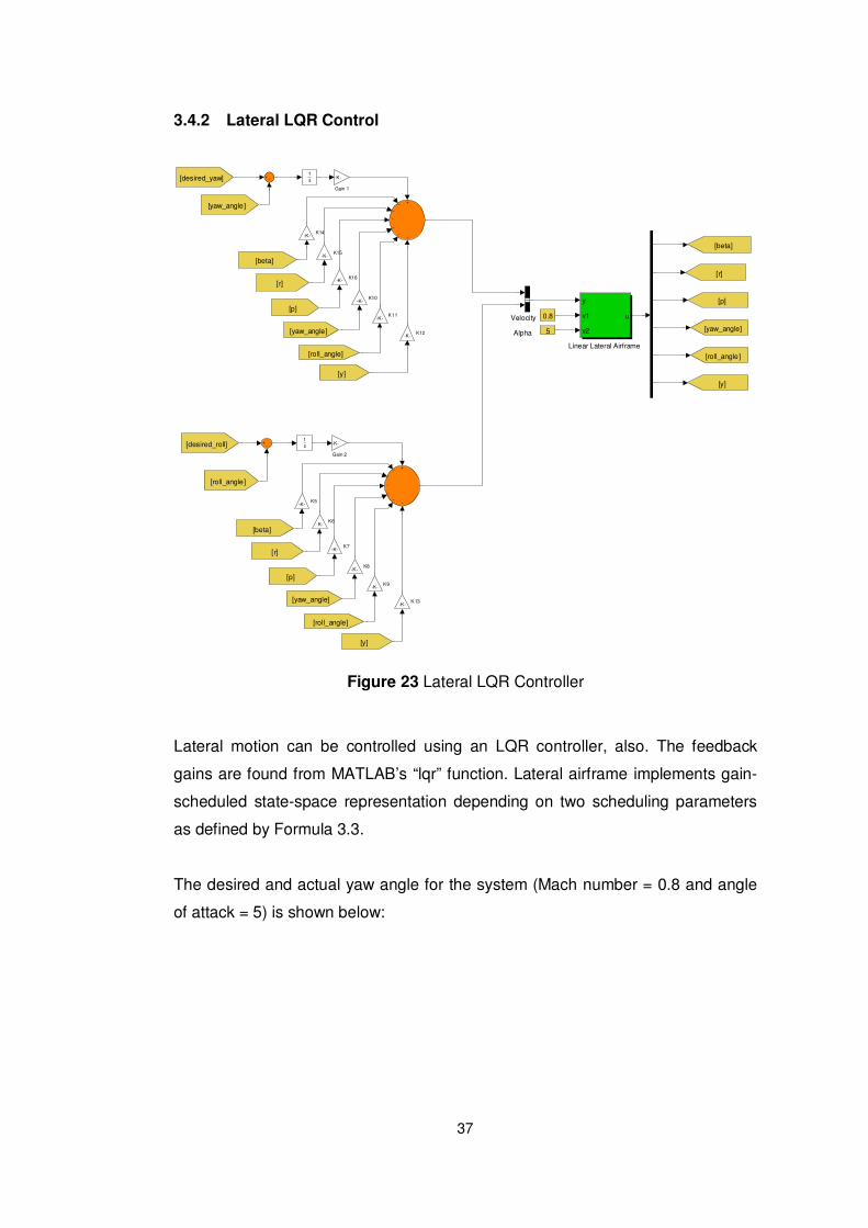
3.4.2 Lateral LQR Control
Velocity
Linear Lateral Airframe
Alpha
1s
K9-K-
K8-K-
K7-K-
K6-K-
K5-K-
K16-K-
K15-K-
K14-K-
K13-K-
K12-K-
K11-K-
K10-K-
1s
[roll_angle]
[p]
[r]
[yaw_angle]
[y]
[beta]
Gain 2
-K-
Gain 1
-K-
[roll_angle]
[yaw_angle]
[p]
[yaw_angle]
[r]
[yaw_angle]
[p]
[beta]
[r]
[y]
[desired_roll]
[roll_angle]
[y]
[beta]
[roll_angle]
[desired_yaw]
0.8
5
y
v1
v2
u
Figure 23 Lateral LQR Controller
Lateral motion can be controlled using an LQR controller, also. The feedback
gains are found from MATLAB’s “lqr” function. Lateral airframe implements gain-
scheduled state-space representation depending on two scheduling parameters
as defined by Formula 3.3.
The desired and actual yaw angle for the system (Mach number = 0.8 and angle
of attack = 5) is shown below:
38
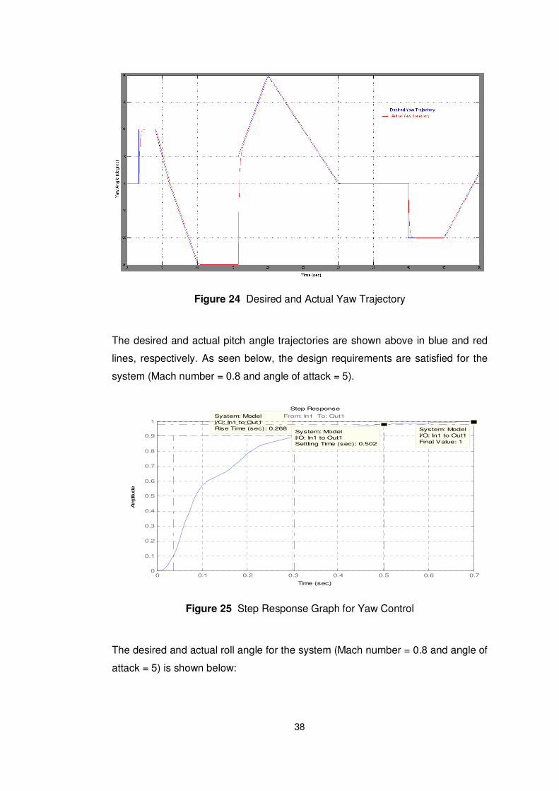
Figure 24 Desired and Actual Yaw Trajectory
The desired and actual pitch angle trajectories are shown above in blue and red
lines, respectively. As seen below, the design requirements are satisfied for the
system (Mach number = 0.8 and angle of attack = 5).
Step Response
Time (sec)
Amplitu
de
0 0.1 0.2 0.3 0.4 0.5 0.6 0.70
0.1
0.2
0.3
0.4
0.5
0.6
0.7
0.8
0.9
1System: ModelI/O: In1 to Out1Rise Time (sec): 0.268 System: Model
I/O: In1 to Out1Final Value: 1
From: In1 To: Out1
System: ModelI/O: In1 to Out1Settling Time (sec): 0.502
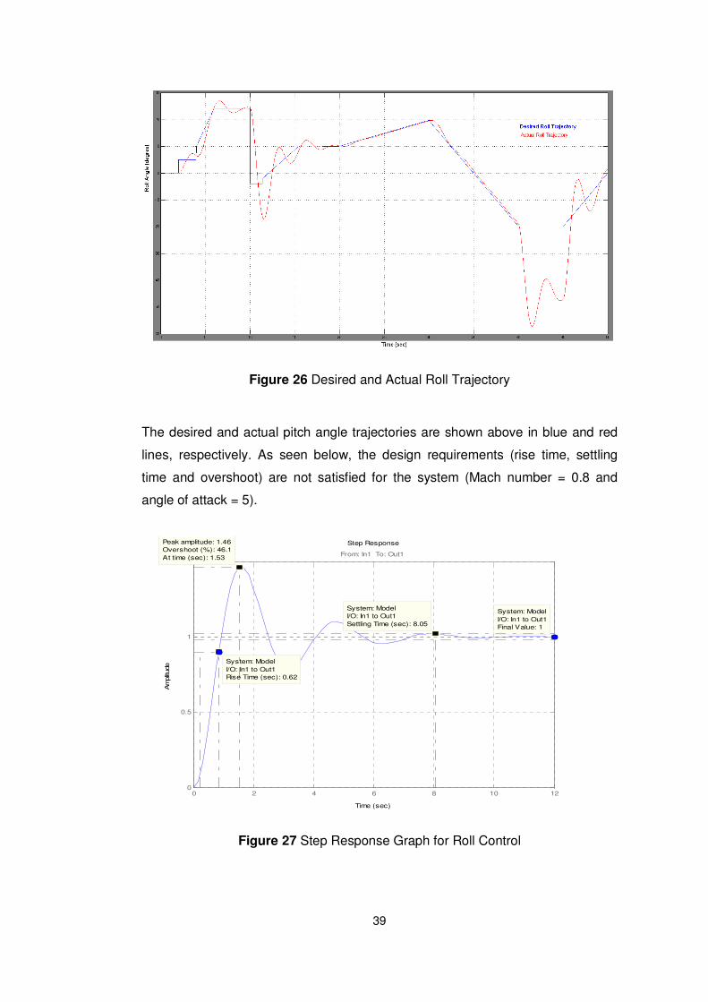
Figure 25 Step Response Graph for Yaw Control
The desired and actual roll angle for the system (Mach number = 0.8 and angle of
attack = 5) is shown below:
39
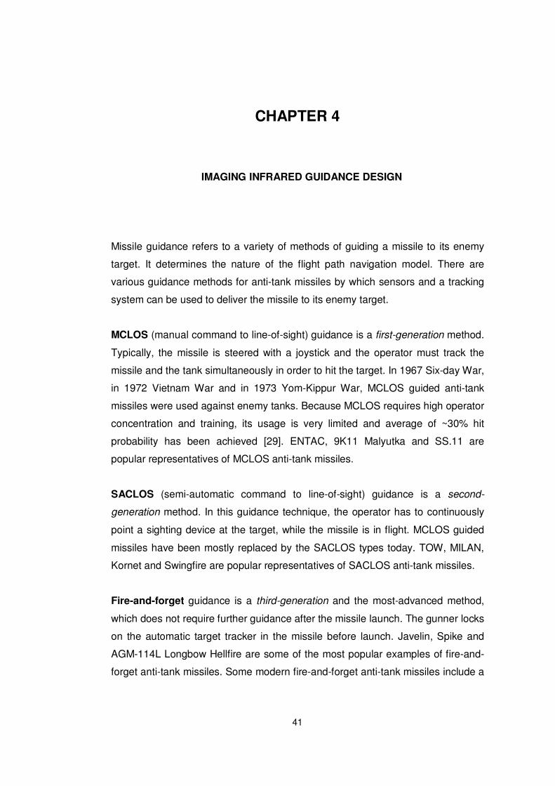
Figure 26 Desired and Actual Roll Trajectory
The desired and actual pitch angle trajectories are shown above in blue and red
lines, respectively. As seen below, the design requirements (rise time, settling
time and overshoot) are not satisfied for the system (Mach number = 0.8 and
angle of attack = 5).
Step Response
Time (sec)
Am
plitu
de
0 2 4 6 8 10 120
0.5
1
1.5
System: ModelI/O: In1 to Out1Final Value: 1
System: ModelI/O: In1 to Out1Rise Time (sec): 0.62
I/O: In1 to Out1Peak amplitude: 1.46Overshoot (%): 46.1At time (sec): 1.53 From: In1 To: Out1
System: ModelI/O: In1 to Out1Settling Time (sec): 8.05
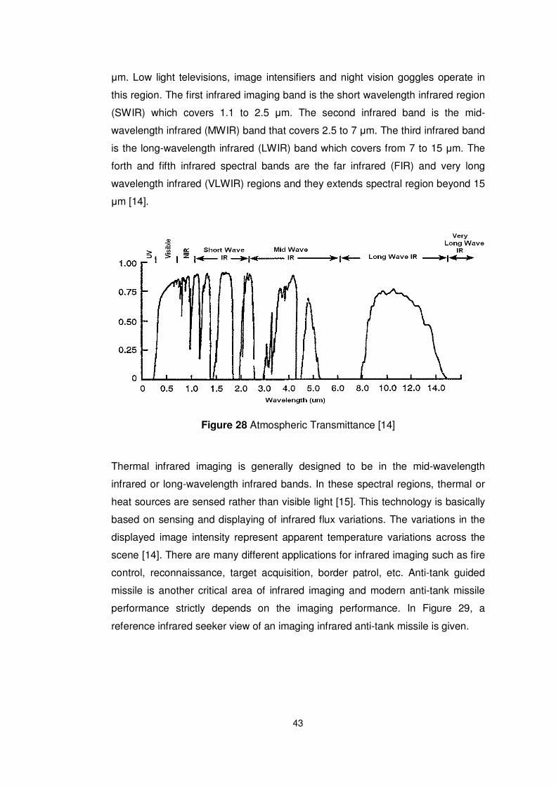
Figure 27 Step Response Graph for Roll Control

40
PID controller satisfies all of the requirements in both planes; however LQR
controller does not satisfy roll control requirements in the lateral plane. Therefore,
PID controller is selected as the basic autopilot controller in the following sections.
41
CHAPTER 4
4 IMAGING INFRARED GUIDANCE DESIGN
Missile guidance refers to a variety of methods of guiding a missile to its enemy
target. It determines the nature of the flight path navigation model. There are
various guidance methods for anti-tank missiles by which sensors and a tracking
system can be used to deliver the missile to its enemy target.
MCLOS (manual command to line-of-sight) guidance is a first-generation method.
Typically, the missile is steered with a joystick and the operator must track the
missile and the tank simultaneously in order to hit the target. In 1967 Six-day War,
in 1972 Vietnam War and in 1973 Yom-Kippur War, MCLOS guided anti-tank
missiles were used against enemy tanks. Because MCLOS requires high operator
concentration and training, its usage is very limited and average of ~30% hit
probability has been achieved [29]. ENTAC, 9K11 Malyutka and SS.11 are
popular representatives of MCLOS anti-tank missiles.
SACLOS (semi-automatic command to line-of-sight) guidance is a second-
generation method. In this guidance technique, the operator has to continuously
point a sighting device at the target, while the missile is in flight. MCLOS guided
missiles have been mostly replaced by the SACLOS types today. TOW, MILAN,
Kornet and Swingfire are popular representatives of SACLOS anti-tank missiles.
Fire-and-forget guidance is a third-generation and the most-advanced method,
which does not require further guidance after the missile launch. The gunner locks
on the automatic target tracker in the missile before launch. Javelin, Spike and
AGM-114L Longbow Hellfire are some of the most popular examples of fire-and-
forget anti-tank missiles. Some modern fire-and-forget anti-tank missiles include a

42
data link between the missile and the launcher platform, which allows the gunner
to watch the video taken by the missile seeker in flight and update the target
information as well as fire-and-forget capability. SPIKE family is an example for
that concept.
Developed first-generation command-guided and second-generation semi-
automatic command guided missiles had many disadvantages and lower hit rates.
For that reason, third generation imaging infrared fire-and-forget anti-tank missile
concept is very popular nowadays.
In this thesis, the anti-tank missile is considered to be a fire and forget type with
update capability. Therefore, the gunner does not need to lock-on the target
before launch, but can choose and lock on the target after launch.
In this chapter, major components of fire-and-forget guidance method are
developed.
4.1 Imaging Infrared Seeker Model
In order to hit the enemy target, it is vital to get correct information about the
target during the missile flight. For imaging infrared fire-and-forget anti-tank
missiles, that information is provided by a seeker. A typical seeker consists of
three major components: (1) An imaging system, (2) a gimbal, and (3) a
processor [2].
4.1.1 Infrared Imaging System
Every object in nature emits radiation, which spread over a frequency spectrum.
Due to atmospheric spectral transmittance, there are seven regions in the
spectrum as described in Figure 28, which should be considered in the design of
an electronic imaging system. The ultraviolet region ranges in wavelength from
0.2 to 0.4 µm. The visible spectrum region ranges in wavelength from 0.4 to 0.7
µm. Televisions, human-eye and most solid state cameras operate in this region.
The near infrared imaging spectral region (NIR) spans approximately 0.7 to 1.1
43
µm. Low light televisions, image intensifiers and night vision goggles operate in
this region. The first infrared imaging band is the short wavelength infrared region
(SWIR) which covers 1.1 to 2.5 µm. The second infrared band is the mid-
wavelength infrared (MWIR) band that covers 2.5 to 7 µm. The third infrared band
is the long-wavelength infrared (LWIR) band which covers from 7 to 15 µm. The
forth and fifth infrared spectral bands are the far infrared (FIR) and very long
wavelength infrared (VLWIR) regions and they extends spectral region beyond 15
µm [14].
Figure 28 Atmospheric Transmittance [14]
Thermal infrared imaging is generally designed to be in the mid-wavelength
infrared or long-wavelength infrared bands. In these spectral regions, thermal or
heat sources are sensed rather than visible light [15]. This technology is basically
based on sensing and displaying of infrared flux variations. The variations in the
displayed image intensity represent apparent temperature variations across the
scene [14]. There are many different applications for infrared imaging such as fire
control, reconnaissance, target acquisition, border patrol, etc. Anti-tank guided
missile is another critical area of infrared imaging and modern anti-tank missile
performance strictly depends on the imaging performance. In Figure 29, a
reference infrared seeker view of an imaging infrared anti-tank missile is given.
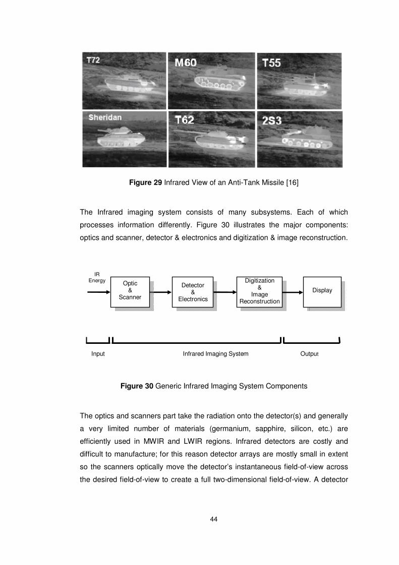
44
Figure 29 Infrared View of an Anti-Tank Missile [16]
The Infrared imaging system consists of many subsystems. Each of which
processes information differently. Figure 30 illustrates the major components:
optics and scanner, detector & electronics and digitization & image reconstruction.
Figure 30 Generic Infrared Imaging System Components
The optics and scanners part take the radiation onto the detector(s) and generally
a very limited number of materials (germanium, sapphire, silicon, etc.) are
efficiently used in MWIR and LWIR regions. Infrared detectors are costly and
difficult to manufacture; for this reason detector arrays are mostly small in extent
so the scanners optically move the detector’s instantaneous field-of-view across
the desired field-of-view to create a full two-dimensional field-of-view. A detector
Digitization &
Image Reconstruction
Display
Detector &
Electronics
Optic &
Scanner
IR Energy
Input
Infrared Imaging System
Output

45
is the hearth of every optical system because it converts scene radiation into a
measurable electrical signal. Amplification and signal processing creates an
electronic image in which voltage differences represent scene intensity
differences due to the various objects in the field-of-view. Signals are then
digitized because of the relative ease to manipulate. Current systems run
software such as gain-level normalization, image enhancement and gamma
correction algorithms after digitization. Finally, scene image is reconstructed again
and displayed on the monitor [14]. For an anti-tank imaging infrared missile,
display is on the launcher platform (helicopter or land vehicle), so video is
transferred via fiber-optic cable or radio frequency datalink between the missile
and the launcher platform. Usually, a human operator views the display and tries
to make a decision as to the existence of a target.
Target acquisition performance depends on many parameters such as detector
resolution, sensitivity, optics, spectral response, A/D performance, human eye
response, display type, etc. In general increasing the range decreases the
acquisition performance, since the number of pixels on the target decreases as a
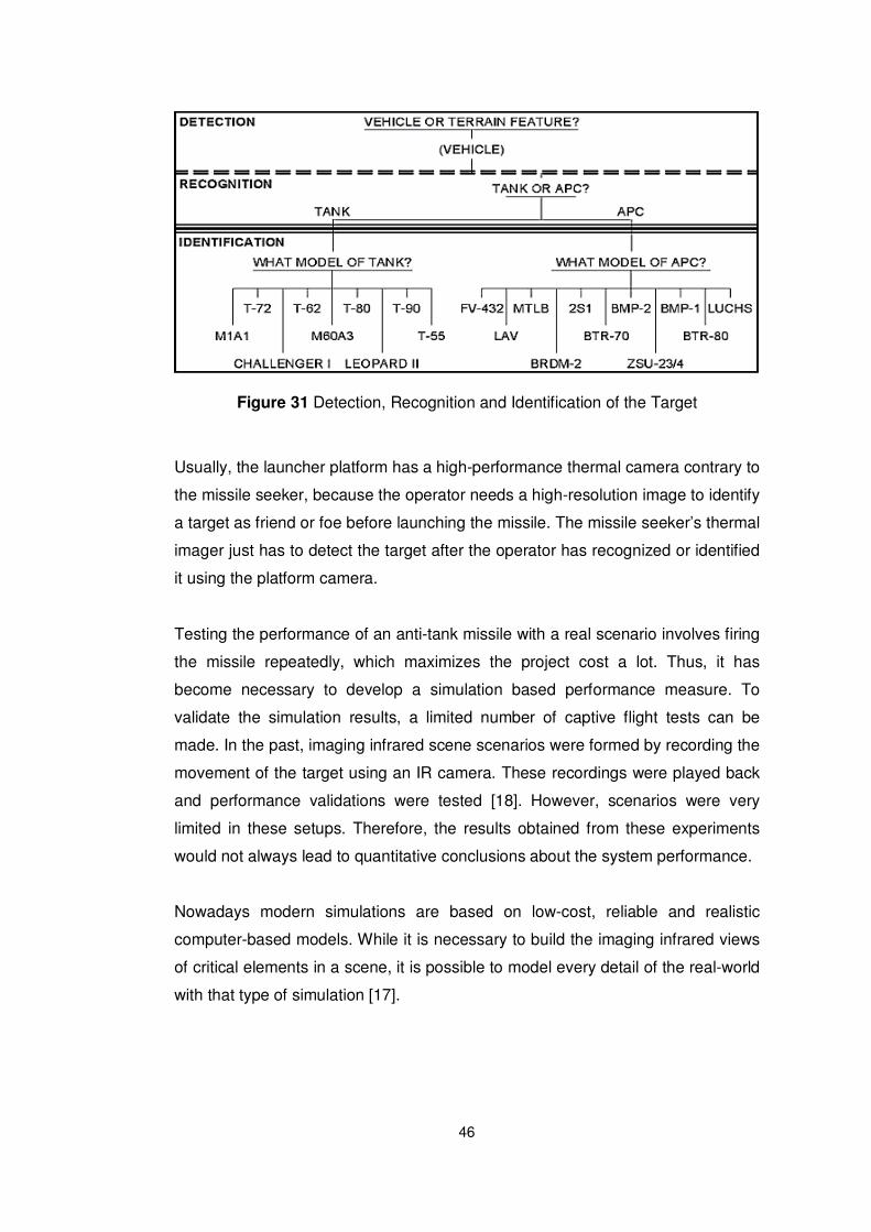
function of range. The first task is searching the field-of-view to find a target. It
varies on observer training and response characteristics. Operator decides
whether suspicious hot spot is a vehicle or a terrain feature on detection level.
After detection, attention is focused on a particular area of the scene. As the
amount of detail perceived by the observer increases, the class to which the
object belongs (tank, tuck, APC, etc.) becomes more clear in the recognition level.
Finally, the target is discerned with sufficient clarity to specify the type (M60, T52,
etc.) in the identification level as described in Figure 31.
46
Figure 31 Detection, Recognition and Identification of the Target
Usually, the launcher platform has a high-performance thermal camera contrary to
the missile seeker, because the operator needs a high-resolution image to identify
a target as friend or foe before launching the missile. The missile seeker’s thermal
imager just has to detect the target after the operator has recognized or identified
it using the platform camera.
Testing the performance of an anti-tank missile with a real scenario involves firing
the missile repeatedly, which maximizes the project cost a lot. Thus, it has
become necessary to develop a simulation based performance measure. To
validate the simulation results, a limited number of captive flight tests can be
made. In the past, imaging infrared scene scenarios were formed by recording the
movement of the target using an IR camera. These recordings were played back
and performance validations were tested [18]. However, scenarios were very
limited in these setups. Therefore, the results obtained from these experiments
would not always lead to quantitative conclusions about the system performance.
Nowadays modern simulations are based on low-cost, reliable and realistic
computer-based models. While it is necessary to build the imaging infrared views
of critical elements in a scene, it is possible to model every detail of the real-world
with that type of simulation [17].
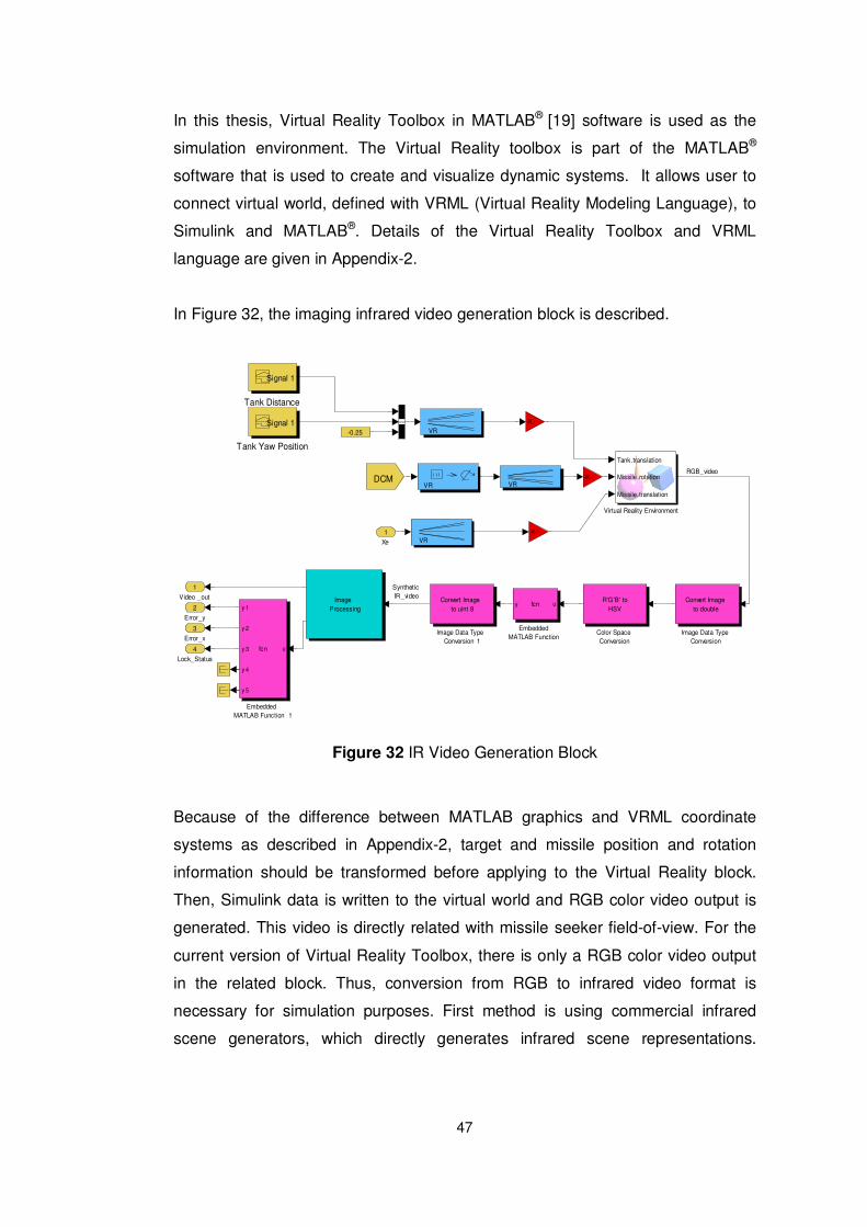
47
In this thesis, Virtual Reality Toolbox in MATLAB® [19] software is used as the
simulation environment. The Virtual Reality toolbox is part of the MATLAB®
software that is used to create and visualize dynamic systems. It allows user to
connect virtual world, defined with VRML (Virtual Reality Modeling Language), to
Simulink and MATLAB®. Details of the Virtual Reality Toolbox and VRML
language are given in Appendix-2.
In Figure 32, the imaging infrared video generation block is described.
RGB_video
Synthetic IR_video
Lock_Status
4
Error_x
3
Error_y
2
Video _out
1
Virtual Reality Environment
Tank.translation
Missile.rotation
Missile.translation
VR
VR
VR
Tank Yaw Position
Signal 1
Tank Distance
Signal 1
VR
Image Processing
Image Data TypeConversion 1
Convert Imageto uint 8
Image Data TypeConversion
Convert Imageto double
-K-
-K-
-K-DCM
EmbeddedMATLAB Function 1
u
y 1
y 2
y 3
y 4
y 5
fcn
EmbeddedMATLAB Function
uy fcn
-0.25
Color Space Conversion
R'G'B' toHSV
Xe
1
Figure 32 IR Video Generation Block
Because of the difference between MATLAB graphics and VRML coordinate
systems as described in Appendix-2, target and missile position and rotation
information should be transformed before applying to the Virtual Reality block.
Then, Simulink data is written to the virtual world and RGB color video output is
generated. This video is directly related with missile seeker field-of-view. For the
current version of Virtual Reality Toolbox, there is only a RGB color video output
in the related block. Thus, conversion from RGB to infrared video format is
necessary for simulation purposes. First method is using commercial infrared
scene generators, which directly generates infrared scene representations.
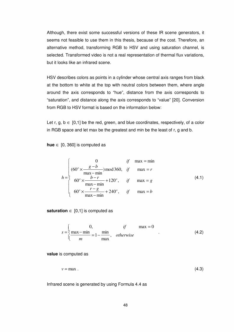
48
Although, there exist some successful versions of these IR scene generators, it
seems not feasible to use them in this thesis, because of the cost. Therefore, an
alternative method, transforming RGB to HSV and using saturation channel, is
selected. Transformed video is not a real representation of thermal flux variations,
but it looks like an infrared scene.
HSV describes colors as points in a cylinder whose central axis ranges from black
at the bottom to white at the top with neutral colors between them, where angle
around the axis corresponds to “hue”, distance from the axis corresponds to
“saturation”, and distance along the axis corresponds to “value” [20]. Conversion
from RGB to HSV format is based on the information below:
Let r, g, b ∈ [0,1] be the red, green, and blue coordinates, respectively, of a color
in RGB space and let max be the greatest and min be the least of r, g and b.
hue ∈ [0, 360] is computed as
=+−
−×
=+−
−×
=−
−×
=
=
bifgr
gifrb
rifbg
if
h
oo
oo
o
max,240minmax
60
max,120minmax
60
max,360mod)minmax
60(
minmax0
(4.1)
saturation ∈ [0,1] is computed as
−=−
==
otherwisem
if
s,
max
min1
minmax
0max,0
. (4.2)
value is computed as
max=v . (4.3)
Infrared scene is generated by using Formula 4.4 as
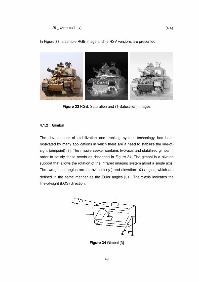
49
)1(_ ssceneIR −= . (4.4)
In Figure 33, a sample RGB image and its HSV versions are presented.
Figure 33 RGB, Saturation and (1-Saturation) Images
4.1.2 Gimbal
The development of stabilization and tracking system technology has been
motivated by many applications in which there are a need to stabilize the line-of-
sight (aimpoint) [3]. The missile seeker contains two-axis and stabilized gimbal in
order to satisfy these needs as described in Figure 34. The gimbal is a pivoted
support that allows the rotation of the infrared imaging system about a single axis.
The two gimbal angles are the azimuth (ψ ) and elevation (θ ) angles, which are
defined in the same manner as the Euler angles [21]. The x-axis indicates the
line-of-sight (LOS) direction.
Figure 34 Gimbal [3]
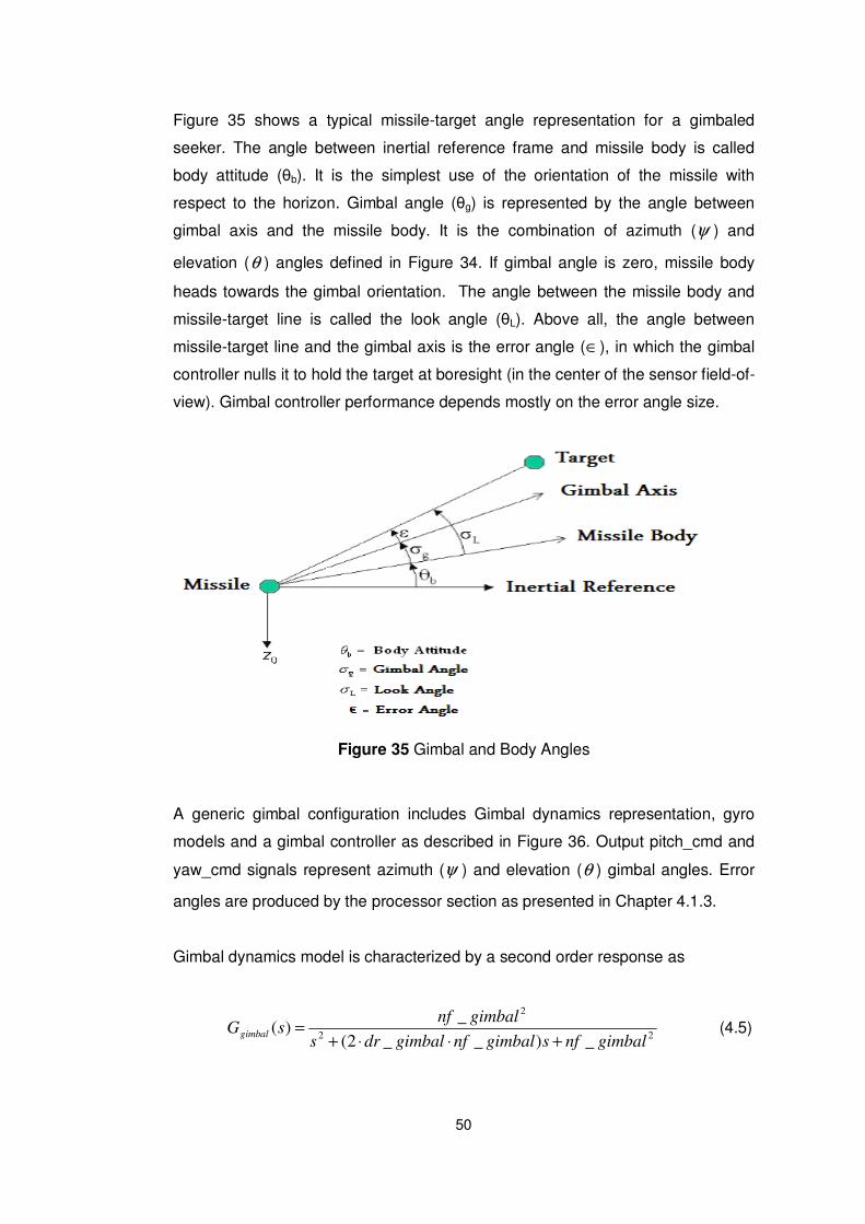
50
Figure 35 shows a typical missile-target angle representation for a gimbaled
seeker. The angle between inertial reference frame and missile body is called
body attitude (θb). It is the simplest use of the orientation of the missile with
respect to the horizon. Gimbal angle (θg) is represented by the angle between
gimbal axis and the missile body. It is the combination of azimuth (ψ ) and
elevation (θ ) angles defined in Figure 34. If gimbal angle is zero, missile body
heads towards the gimbal orientation. The angle between the missile body and
missile-target line is called the look angle (θL). Above all, the angle between
missile-target line and the gimbal axis is the error angle (∈), in which the gimbal
controller nulls it to hold the target at boresight (in the center of the sensor field-of-
view). Gimbal controller performance depends mostly on the error angle size.
Figure 35 Gimbal and Body Angles
A generic gimbal configuration includes Gimbal dynamics representation, gyro
models and a gimbal controller as described in Figure 36. Output pitch_cmd and
yaw_cmd signals represent azimuth (ψ ) and elevation (θ ) gimbal angles. Error
angles are produced by the processor section as presented in Chapter 4.1.3.
Gimbal dynamics model is characterized by a second order response as
22
2
_)__2(
_)(
gimbalnfsgimbalnfgimbaldrs
gimbalnfsGgimbal
+⋅⋅+= (4.5)

51
where natural frequency of the gimbal (nf_gimbal) is 320Hz and the damping ratio
of gimbal (dr_gimbal) is 0.7. Gyro dynamics model is also characterized by a
second order response as
22
2
_)__2(
_)(
gyronfsgyronfgyrodrs
gyronfsGgyro
+⋅⋅+= (4.6)
where natural frequency of gyro (nf_gyro) is 620Hz and the damping ratio of gyro
(dr_gyro) is 0.7.
yaw_cmd
2
pitch _cmd
1
PID PID
PIDPID
1s
1s
Gyro Dynamics Model
nf_gyro^2
s +2*dr_gyro *nf_gyros+nf_gyro^22
Gyro Dynamics Model
nf_gyro^2
s +2*dr_gyro *nf_gyros+nf_gyro^22
Gimbal Dynamics Model 1
nf_gimbal ^2
s +2*dr_gimbal *nf_gimbals +nf_gimbal ^22
Gimbal Dynamics Model
nf_gimbal ^2
s +2*dr_gimbal *nf_gimbals +nf_gimbal ^22
r
q
Error_x
2
Error_y
1
Figure 36 Gimbal Dynamics Representation
Gyro is perhaps the most critical component of the gimbal system. Its dynamic
characteristics largely determine the control system bandwidth and system
performance that can be achieved [3]. The azimuth gyro has its input axis along
the x-axis, and drive the gimbal system about the z-axis, and the elevation gyro
has its input axis along the y-axis [21]. For longitudinal orientation, y-axis angular
rate (q) is added to the gyro response in order to insert the missile body angular
effects to the gimbal dynamics; and for lateral orientation, z-axis angular rate (r) is
added to the gyro response in order to insert the missile body angular effects to
the gimbal dynamics.
52
There exist two gimbal controllers for longitudinal and lateral dynamic parts,
respectively. First controller (proportional controller) is called the tracking
controller; longitudinal part nulls the y-axis error angle (in pixel) and lateral part
nulls the x-axis error angle (in pixel). Inner controller is called the stabilization
controller, which stabilizes the target in the center of the sensor field-of-view. This
inner controller is selected as a PI (proportional integral) controller. Response
Optimization of Simulink is used for determining the gain values for P and PI
parameters.
4.1.3 Processor
For an anti-tank imaging infrared missile, one of the most critical issues to provide
high target kill probability is the tracking performance, running in the processor
section. Tracking systems are employed in a wide variety of environments. They
are used in numerous applications including fire control, navigation and missile
guidance.
In a typical closed loop imaging infrared tracker, the input to the processor
subsystem is the infrared video and the output is the angular displacement
between the measured target LOS and the gimbal axis [22].
Many different methods of target tracking algorithms have been developed, but
fundamental, simple and reliable algorithms, centroid and correlation, are
frequently used in missile applications. Moreover, active contour (snake) method
is studied in this thesis, additionally.
4.1.3.1 Centroid Tracker
Centroid tracker is based on target/background classification and target’s centroid
computation using target and background histograms. It typically operates by
applying a threshold to the image to segment the scene into target and
background regions. The threshold is usually updated during missile flight. Once
target pixels are estimated, the centroid can be determined as the weighted

53
average of measured intensities [22]. Then the gate position and size are updated
according to the centroid coordinates. These steps are presented in Figure 37
and discussed in the following sections.
Figure 37 Centroid Algorithm
4.1.3.1.1 Finding Target and Background Histograms
In every frame, centroid tracker estimates new target position and background
gates according to the target gate as described in Figure 38. Gating reduces the
number of operations that must be performed to determine the target position. In
addition to this, effects of noise and clutter on the tracking process are largely
suppressed by using target and background gates [2].
Figure 38 Target and Background Gates
Finding Target and Background
Histograms
IR Video
Estimating Target Pixels
Computing Target’s Centroid
Updating Gate Position & Size
Target Position
54
In the implementations in this study, there exist one target gate and four
background gates, in which histograms are computed. Histogram shows intensity
distribution of gates. Previous and current frame’s target and background
histograms are correlated using the Formula 4.7, because current histograms can
be unreliable in some frames.
[ ] [ ]( ) [ ]
[ ] [ ]( ) [ ] __Pr1
__
_arg_Pr1
_arg_arg
iHistogramBackgroundevious
iHistogramBackgroundiHistogramBackground
iHistogrametTevious
iHistogrametTiHistogrametT
×−
+×=
×−
+×=
γ
γ
γ
γ
(4.7)
where 0 < γ < 1 is update rate. While γ increases, histogram update rate
increases as well.
4.1.3.1.2 Estimating Target Pixels
After finding target and background histograms, target probability distribution
(TPD) is computed by using Formula 4.8 as,
][_][_arg
][_arg][
iHistogramBackgroundiHistogrametT
iHistogrametTiTPD
+= (4.8)
where i is the intensity and it takes values between 0 and 255 for an 8-bit infrared
video density.
TPD becomes 1 only within the target histogram. Example histogram graphs and
related target probability distribution are presented in Figure 39.
55
Figure 39 Histogram Analysis
Using target probability distribution, target pixels are found by considering the
target threshold. Intensity values bigger than the threshold are considered as
target pixels. Thresholding is critical to separate the target from the background,
effectively. Therefore, the target threshold should be updated during missile flight
in a logical way.
Threshold selection can be based on (1) Histograms Method, (2) Target and
Background Gate Method, and (3) Peak and Average Method [23].
In Histogram Method, threshold is found using scene histogram information.
This method is applicable if the histogram is bimodal, i.e. two distinct local
maxima in the histogram distribution exist. A suitable threshold value can be
chosen within these two maxima. However, in general, distributions are not
56
bimodal, so the threshold selection becomes very difficult [23]. Therefore, this
method is discarded.
In Target and Background Gate Approach, target and background average
intensity levels are computed using Formula 4.9 as
Y
i
AverageBackground
T
i
AverageetT
GateBackground
PixelsetT
∑
∑
=
=
_
_arg
_
_arg
(4.9)
where T is the number of target pixels and Y is the number of pixels enclosed in
the background gate. Threshold is between the target and background averages
and is usually mean of the two.
In Peak and Average Method, peak and average intensity level of complete
scene including target and background are computed. Threshold is fixed in
between the average and the peak and is usually mean of the two.
Thresholding is optimized by combining the second and third approaches for the
centroid tracker algorithm. Threshold is found using Peak and Average method for
the first few frames and later by Target and Background method.
4.1.3.1.3 Computing Target’s Centroid
Once target pixels are classified, the centroid can be computed as the weighted
average of target intensities.
∑
∑
×=
×=
GateetT
n
y
GateetT
j
x
T
ync
T
xjc
_arg
_arg (4.10)
57
where T is the number of target pixels, j is the column number, n is the row
number, xj is the x projection of jth column and yn is the y projection of nth row.
Target x and y projections are found for computing centroid coordinates cx and cy
as described in Figure 40, where red point represents the target centroid.
Figure 40 Computing Centroid Coordinates
4.1.3.1.4 Updating Gate Position and Size
The placement and sizing of target gate affects the ability of computing target
location in the following frame. If the gate is misplaced or is too small, some of the
target can be excluded from target position measurement processing. If it is too
large, then it will include a quantity of background pixels that may interfere with
the computation performance. Therefore, current frame’s characteristics
constitute next frame’s target gate position and size. Position is directly related
with centroid coordinates.
0 0 0 4 8 8 0 0 0
0 0 2 2 3 3 3 3 2 2 0 0
X Projection of
Target Pixels
Y Projection of
Target Pixels
0 1 2 3 4 5 6 7 8
0 1 2 3 4 5 6 7 8 9 1011
cy=[0x0+1x0+2x0+3x4+4x8+5x8+6x0+7x0+8x0]/(0+0+0+4+8+8+0+0+0)=84/20=4.2
cx=[0x0+1x0+2x2+3x2+4x3+5x3+6x3+7x3+8x2+9x2+10x0+11x0]/ (0+0+2+2+3+3+3+3+2+2+0+0)=105/20=5.25
58
One of the most advantageous characteristics of the centroid tracker is the
adaptation capability of enlarging or shrinking targets according to Formula 4.11
as,
( )
( ))__(
)__(_
)__(
)__(_
12
12
buttomsearchupsearchrow
buttomsearchupsearchrowgytotalgk
leftsearchrightsearchcolumn
leftsearchrightsearchcolumngxtotalgk
y
x
⋅⋅
⋅⋅×−×=
⋅⋅
⋅⋅×−×=
(4.11)
where g2 is the changing rate, g1 is the enclosing rate, column is the total column
quantity in gate, row is the total row quantity in gate, search_up is the total
number of upper search columns, search_buttom is the total number of buttom
search columns, total_x is the total target pixels in search columns, total_y is the
total target pixels in search rows, search_right is the total number of right search
rows and search_left is the total number of left search rows.
For both x and y axes, if target is enlarging in one direction and target pixels are
increasing respectively, then the gate size is adjusted as described with an
example in Figure 41 as,
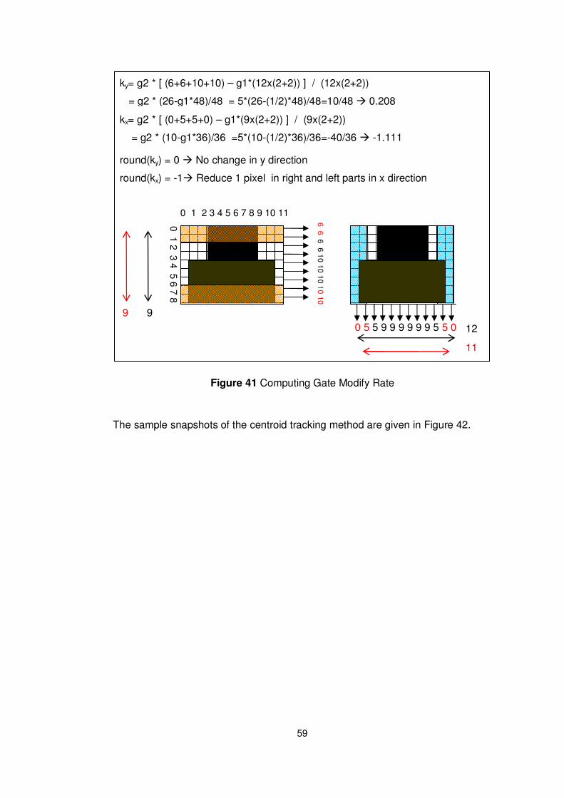
59
Figure 41 Computing Gate Modify Rate
The sample snapshots of the centroid tracking method are given in Figure 42.
0 1 2 3 4 5 6 7 8
0 1 2 3 4 5 6 7 8 9 10 11
0 5 5 9 9 9 9 9 9 5 5 0
kx= g2 * [ (0+5+5+0) – g1*(9x(2+2)) ] / (9x(2+2))
= g2 * (10-g1*36)/36 =5*(10-(1/2)*36)/36=-40/36 -1.111
12
11
9 9
6 6 6 6 10 10
10 1
0 10
ky= g2 * [ (6+6+10+10) – g1*(12x(2+2)) ] / (12x(2+2))
= g2 * (26-g1*48)/48 = 5*(26-(1/2)*48)/48=10/48 0.208
round(ky) = 0 No change in y direction
round(kx) = -1 Reduce 1 pixel in right and left parts in x direction
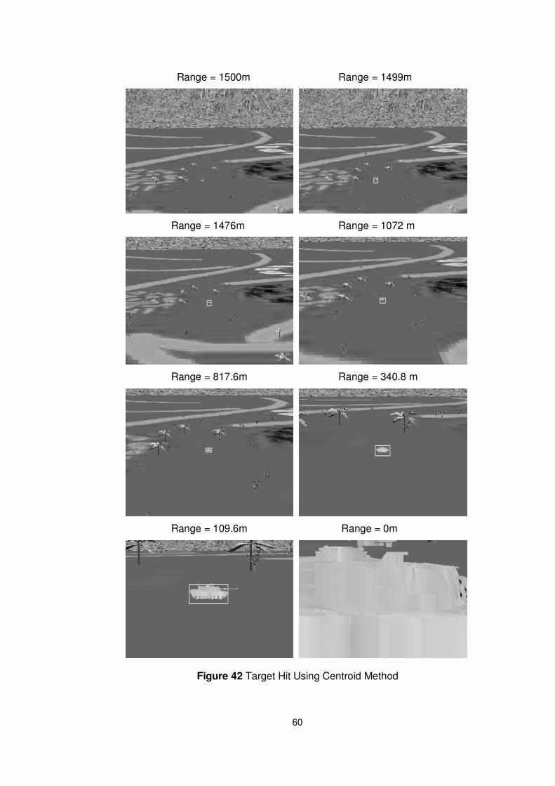
60
Range = 1500m Range = 1499m
Range = 1476m Range = 1072 m
Range = 817.6m Range = 340.8 m
Range = 109.6m Range = 0m
Figure 42 Target Hit Using Centroid Method
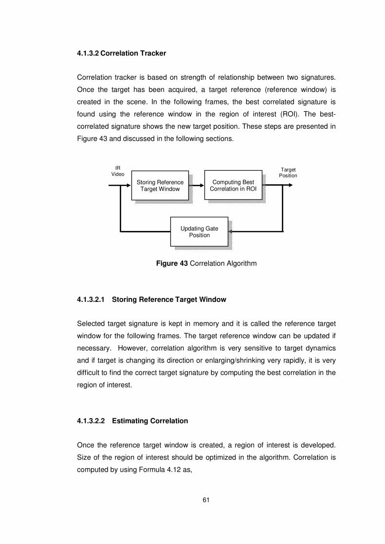
61
4.1.3.2 Correlation Tracker
Correlation tracker is based on strength of relationship between two signatures.
Once the target has been acquired, a target reference (reference window) is
created in the scene. In the following frames, the best correlated signature is
found using the reference window in the region of interest (ROI). The best-
correlated signature shows the new target position. These steps are presented in
Figure 43 and discussed in the following sections.
Figure 43 Correlation Algorithm
4.1.3.2.1 Storing Reference Target Window
Selected target signature is kept in memory and it is called the reference target
window for the following frames. The target reference window can be updated if
necessary. However, correlation algorithm is very sensitive to target dynamics
and if target is changing its direction or enlarging/shrinking very rapidly, it is very
difficult to find the correct target signature by computing the best correlation in the
region of interest.
4.1.3.2.2 Estimating Correlation
Once the reference target window is created, a region of interest is developed.
Size of the region of interest should be optimized in the algorithm. Correlation is
computed by using Formula 4.12 as,
Storing Reference Target Window
IR Video
Computing Best Correlation in ROI
Updating Gate Position
Target Position
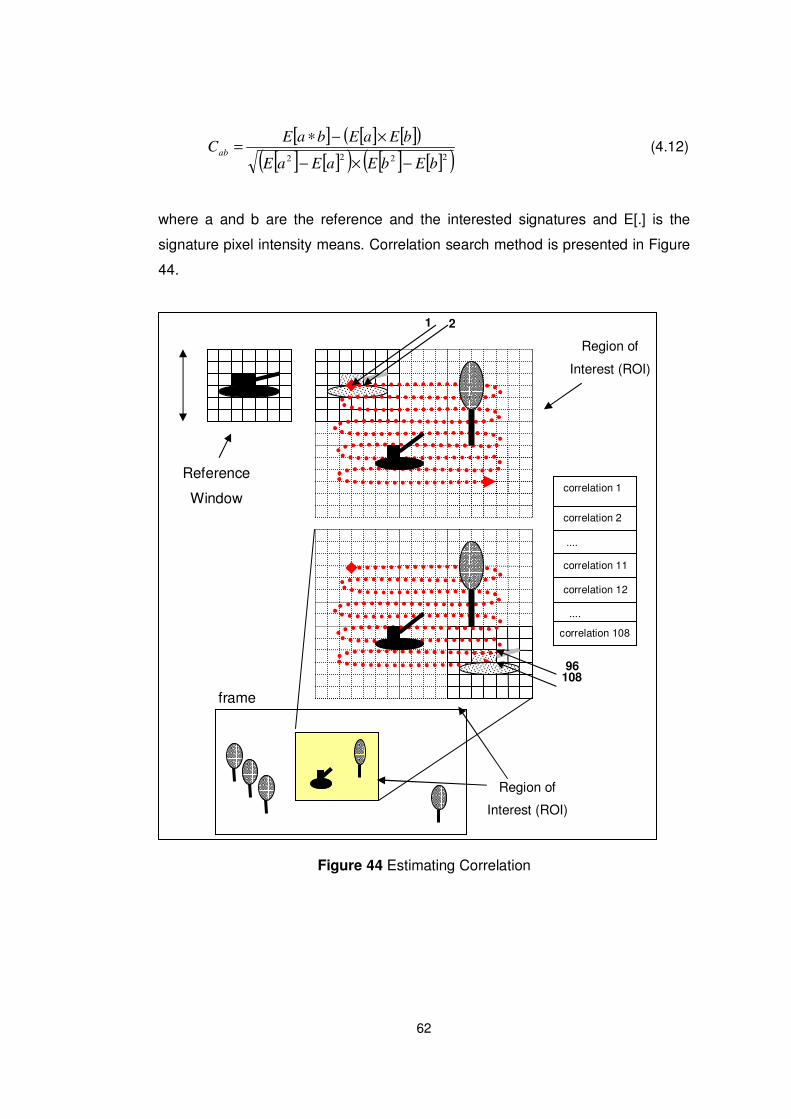
62
[ ] [ ] [ ]( )
[ ] [ ]( ) [ ] [ ]( )2222 bEbEaEaE
bEaEbaEC
ab
−×−
×−∗= (4.12)
where a and b are the reference and the interested signatures and E[.] is the
signature pixel intensity means. Correlation search method is presented in Figure
44.
Figure 44 Estimating Correlation
Reference
Window
1 2
correlation 2
....
correlation 11
correlation 12
....
correlation 108
108 96
frame
Region of
Interest (ROI)
correlation 1
Region of
Interest (ROI)
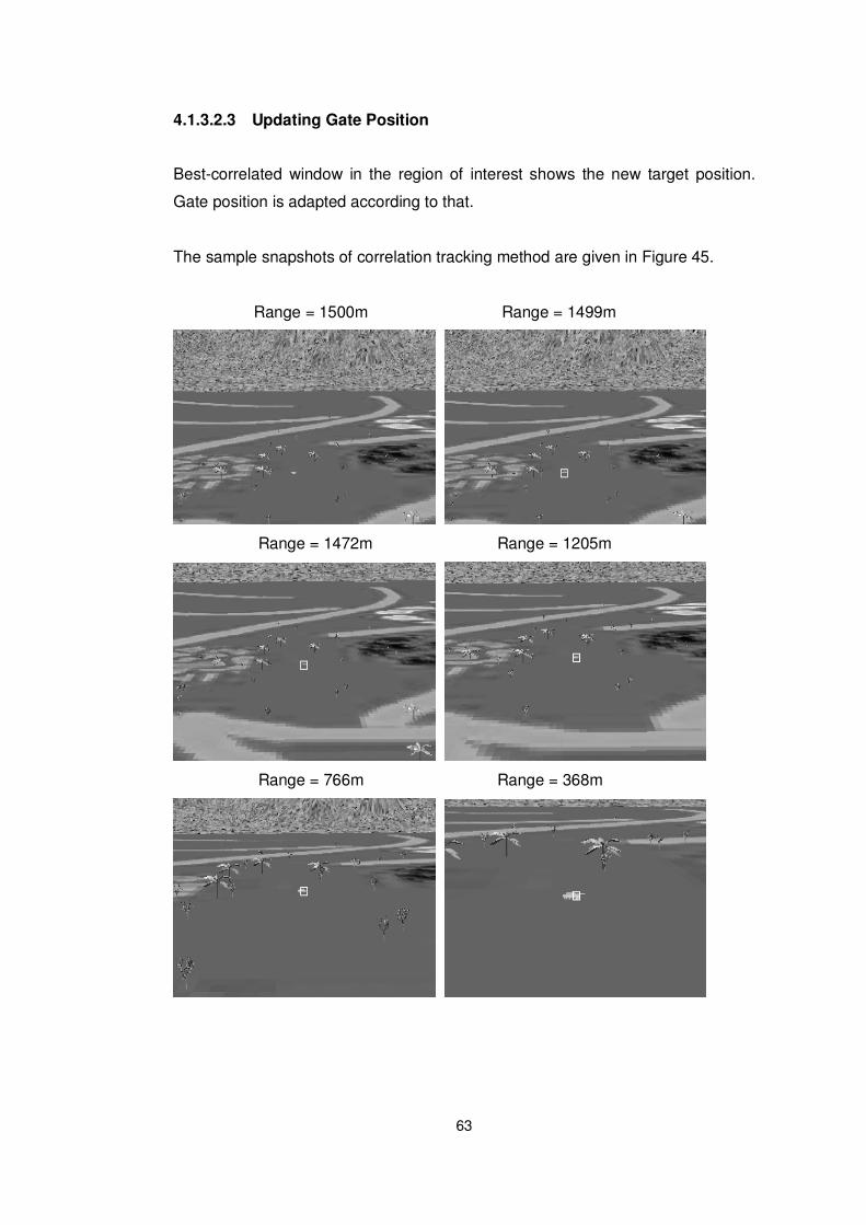
63
4.1.3.2.3 Updating Gate Position
Best-correlated window in the region of interest shows the new target position.
Gate position is adapted according to that.
The sample snapshots of correlation tracking method are given in Figure 45.
Range = 1500m Range = 1499m
Range = 1472m Range = 1205m
Range = 766m Range = 368m
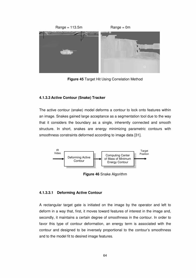
64
Range = 113.5m Range = 0m
Figure 45 Target Hit Using Correlation Method
4.1.3.3 Active Contour (Snake) Tracker
The active contour (snake) model deforms a contour to lock onto features within
an image. Snakes gained large acceptance as a segmentation tool due to the way
that it considers the boundary as a single, inherently connected and smooth
structure. In short, snakes are energy minimizing parametric contours with
smoothness constraints deformed according to image data [31].
Figure 46 Snake Algorithm
4.1.3.3.1 Deforming Active Contour
A rectangular target gate is initiated on the image by the operator and left to
deform in a way that, first, it moves toward features of interest in the image and,
secondly, it maintains a certain degree of smoothness in the contour. In order to
favor this type of contour deformation, an energy term is associated with the
contour and designed to be inversely proportional to the contour’s smoothness
and to the model fit to desired image features.
Deforming Active Contour
IR Video
Computing Center of Mass of Minimum
Energy Contour
Target Position
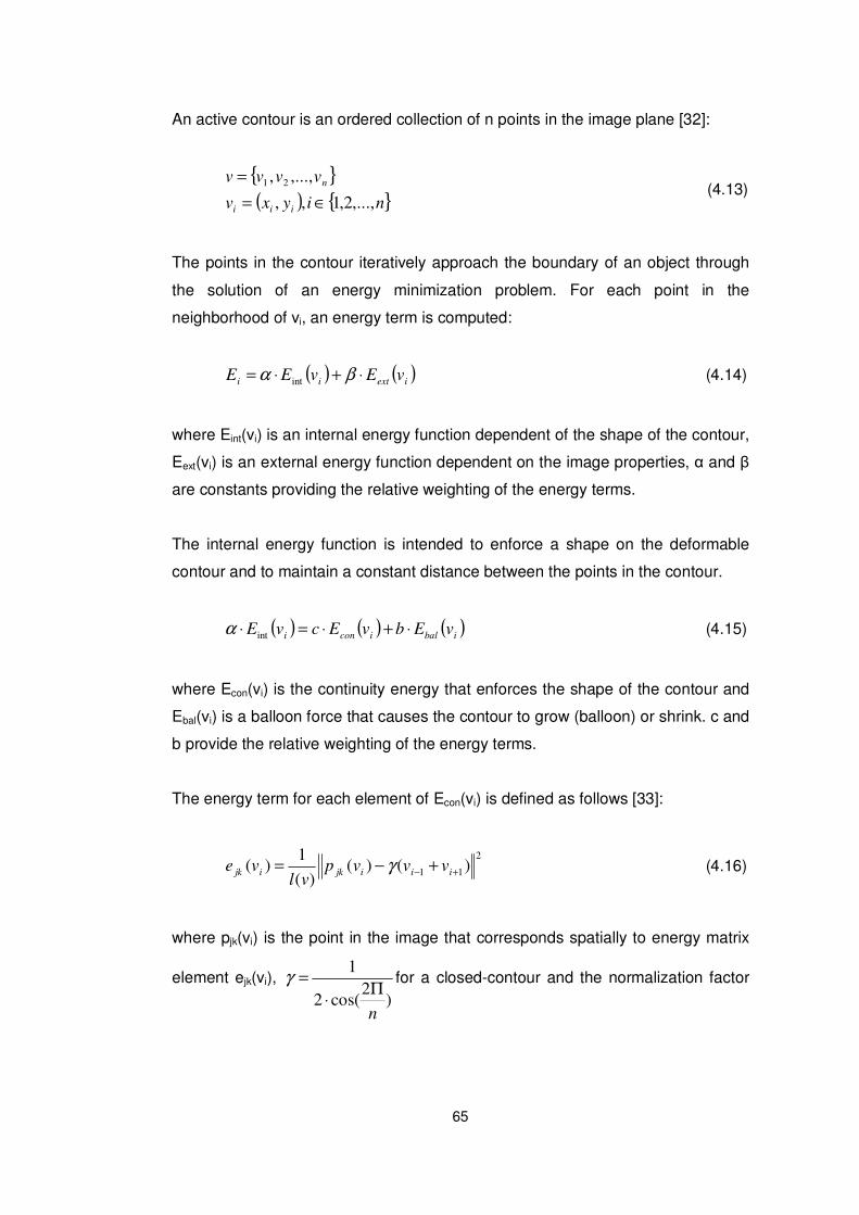
65
An active contour is an ordered collection of n points in the image plane [32]:
( ) niyxv
vvvv
iii
n
,...,2,1,,
,...,, 21
∈=
= (4.13)
The points in the contour iteratively approach the boundary of an object through
the solution of an energy minimization problem. For each point in the
neighborhood of vi, an energy term is computed:
( ) ( )iextii
vEvEE ⋅+⋅= βα int (4.14)
where Eint(vi) is an internal energy function dependent of the shape of the contour,
Eext(vi) is an external energy function dependent on the image properties, α and β
are constants providing the relative weighting of the energy terms.
The internal energy function is intended to enforce a shape on the deformable
contour and to maintain a constant distance between the points in the contour.
( ) ( ) ( )ibaliconi
vEbvEcvE ⋅+⋅=⋅ intα (4.15)
where Econ(vi) is the continuity energy that enforces the shape of the contour and
Ebal(vi) is a balloon force that causes the contour to grow (balloon) or shrink. c and
b provide the relative weighting of the energy terms.
The energy term for each element of Econ(vi) is defined as follows [33]:
2
11 )()()(
1)( +− +−= iiijkijk vvvp
vlve γ (4.16)
where pjk(vi) is the point in the image that corresponds spatially to energy matrix
element ejk(vi), )
2cos(2
1
n
Π⋅
=γ for a closed-contour and the normalization factor
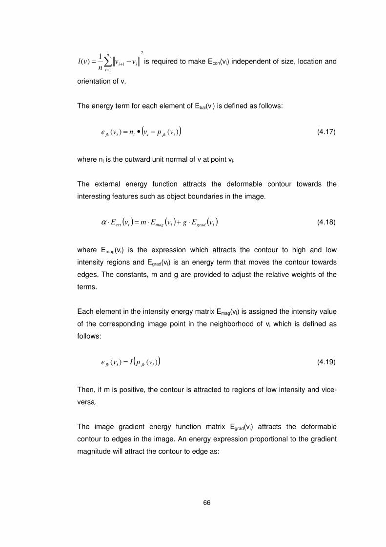
66
2
1
1
1)( ∑
=+ −=
n
i
ii vvn
vl is required to make Econ(vi) independent of size, location and
orientation of v.
The energy term for each element of Ebal(vi) is defined as follows:
( ))()( ijkiiijk vpvnve −•= (4.17)
where ni is the outward unit normal of v at point vi.
The external energy function attracts the deformable contour towards the
interesting features such as object boundaries in the image.
( ) ( ) ( )igradimagiext vEgvEmvE ⋅+⋅=⋅α (4.18)
where Emag(vi) is the expression which attracts the contour to high and low
intensity regions and Egrad(vi) is an energy term that moves the contour towards
edges. The constants, m and g are provided to adjust the relative weights of the
terms.
Each element in the intensity energy matrix Emag(vi) is assigned the intensity value
of the corresponding image point in the neighborhood of vi which is defined as
follows:
( ))()( ijkijk vpIve = (4.19)
Then, if m is positive, the contour is attracted to regions of low intensity and vice-
versa.
The image gradient energy function matrix Egrad(vi) attracts the deformable
contour to edges in the image. An energy expression proportional to the gradient
magnitude will attract the contour to edge as:
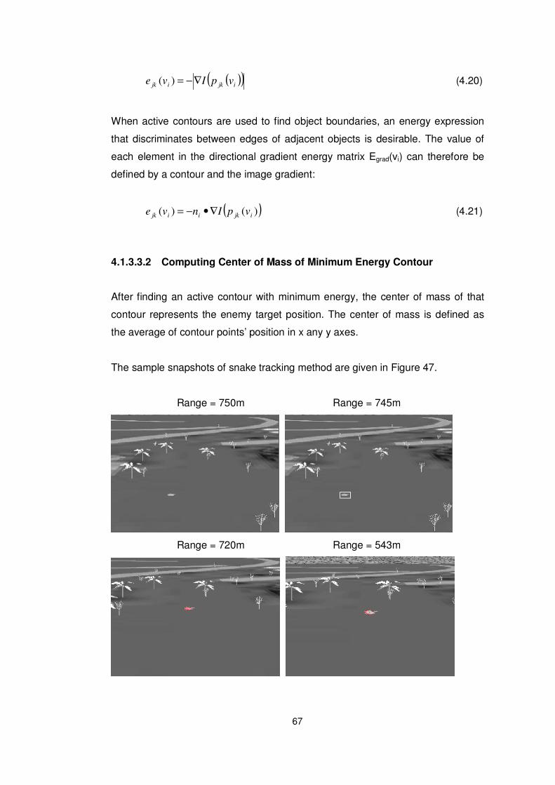
67
( )( )ijkijk vpIve ∇−=)( (4.20)
When active contours are used to find object boundaries, an energy expression
that discriminates between edges of adjacent objects is desirable. The value of
each element in the directional gradient energy matrix Egrad(vi) can therefore be
defined by a contour and the image gradient:
( ))()( ijkiijk vpInve ∇•−= (4.21)
4.1.3.3.2 Computing Center of Mass of Minimum Energy Contour
After finding an active contour with minimum energy, the center of mass of that
contour represents the enemy target position. The center of mass is defined as
the average of contour points’ position in x any y axes.
The sample snapshots of snake tracking method are given in Figure 47.
Range = 750m Range = 745m
Range = 720m Range = 543m
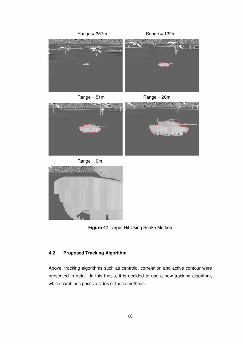
68
Range = 357m Range = 122m
Range = 51m Range = 26m
Range = 0m
Figure 47 Target Hit Using Snake Method
4.2 Proposed Tracking Algorithm
Above, tracking algorithms such as centroid, correlation and active contour were
presented in detail. In this thesis, it is decided to use a new tracking algorithm,
which combines positive sides of these methods.

69
Centroid trackers are most applicable for expanding targets because of gate size
adaptation capability. However, larger targets often have high internal detail,
which are more suitably tracked by correlation or active contour algorithm.
Therefore, when the target occupies a big portion of the scene, active contour
algorithm is switched from centroid method.
Centroid trackers are robust in low-clutter scenarios, with medium-to-high target
SNRs. Centroid algorithm is less effective on lower SNR targets, or in high clutter.
Therefore, when the target is a blob-like small point in the scene, correlation
method is preferred [22].
In the terminal phase, point of impact (POI) is selected as the center of mass of
active contour. Using that information, missile is guided to the high vulnerability
points.
Using above facts, below flow chart is proposed as a new tracking algorithm for
an imaging infrared anti-tank missile application [23]. In the following chapter,
comparison of centroid, correlation, snake and proposed algorithm will be
presented.

70
Figure 48 Proposed Tracking Algorithm Flow Chart
The sample snapshots of proposed tracking method are given in Figure 49.
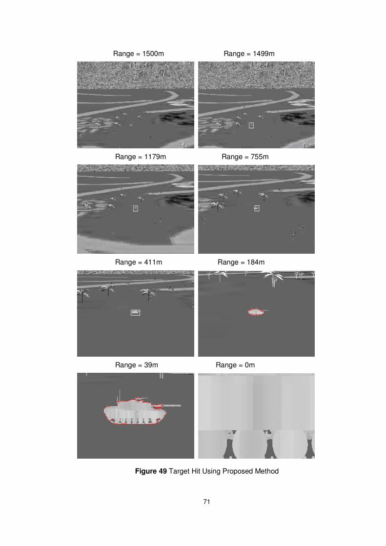
71
Range = 1500m Range = 1499m
Range = 1179m Range = 755m
Range = 411m Range = 184m
Range = 39m Range = 0m
Figure 49 Target Hit Using Proposed Method
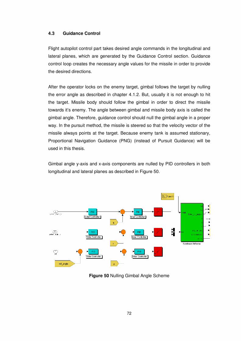
72
4.3 Guidance Control
Flight autopilot control part takes desired angle commands in the longitudinal and
lateral planes, which are generated by the Guidance Control section. Guidance
control loop creates the necessary angle values for the missile in order to provide
the desired directions.
After the operator locks on the enemy target, gimbal follows the target by nulling
the error angle as described in chapter 4.1.2. But, usually it is not enough to hit
the target. Missile body should follow the gimbal in order to direct the missile
towards it’s enemy. The angle between gimbal and missile body axis is called the
gimbal angle. Therefore, guidance control should null the gimbal angle in a proper
way. In the pursuit method, the missile is steered so that the velocity vector of the
missile always points at the target. Because enemy tank is assumed stationary,
Proportional Navigation Guidance (PNG) (instead of Pursuit Guidance) will be
used in this thesis.
Gimbal angle y-axis and x-axis components are nulled by PID controllers in both
longitudinal and lateral planes as described in Figure 50.
Figure 50 Nulling Gimbal Angle Scheme

73
Inner PID controllers were described in chapter 3.3.1 in flight autopilot section.
Response Optimization of Simulink is used for determining gain values for outer
PID controllers. “gimbal_angle_y” and “gimbal_angle_x” angles are produced by
the Gimbal.
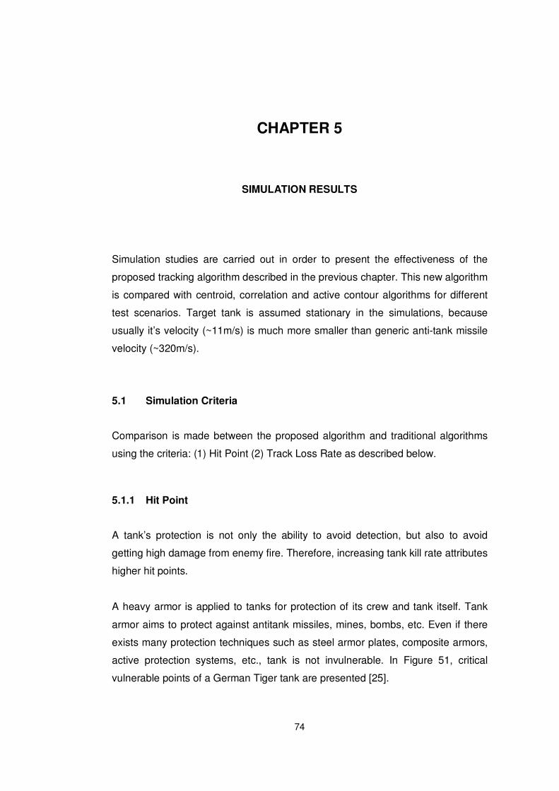
74
CHAPTER 5
5 SIMULATION RESULTS
Simulation studies are carried out in order to present the effectiveness of the
proposed tracking algorithm described in the previous chapter. This new algorithm
is compared with centroid, correlation and active contour algorithms for different
test scenarios. Target tank is assumed stationary in the simulations, because
usually it’s velocity (~11m/s) is much more smaller than generic anti-tank missile
velocity (~320m/s).
5.1 Simulation Criteria
Comparison is made between the proposed algorithm and traditional algorithms
using the criteria: (1) Hit Point (2) Track Loss Rate as described below.
5.1.1 Hit Point
A tank’s protection is not only the ability to avoid detection, but also to avoid
getting high damage from enemy fire. Therefore, increasing tank kill rate attributes
higher hit points.
A heavy armor is applied to tanks for protection of its crew and tank itself. Tank
armor aims to protect against antitank missiles, mines, bombs, etc. Even if there
exists many protection techniques such as steel armor plates, composite armors,
active protection systems, etc., tank is not invulnerable. In Figure 51, critical
vulnerable points of a German Tiger tank are presented [25].
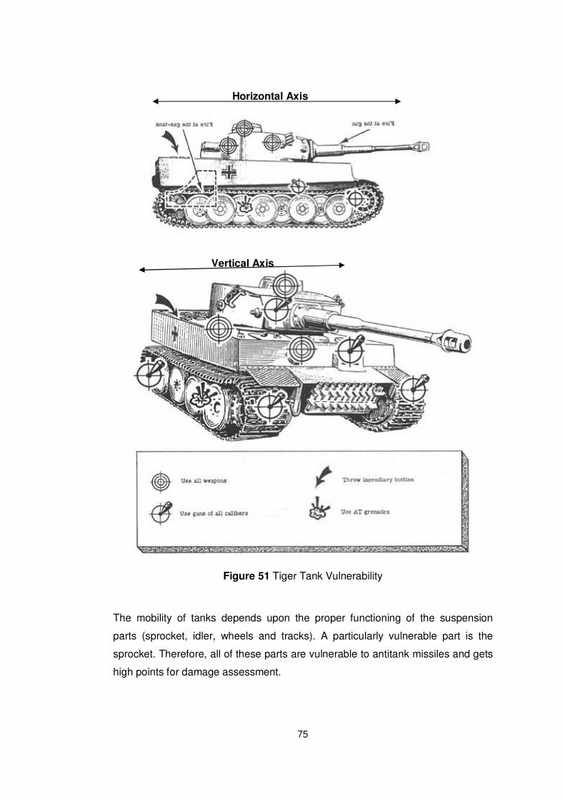
75
Horizontal Axis
Figure 51 Tiger Tank Vulnerability
The mobility of tanks depends upon the proper functioning of the suspension
parts (sprocket, idler, wheels and tracks). A particularly vulnerable part is the
sprocket. Therefore, all of these parts are vulnerable to antitank missiles and gets
high points for damage assessment.
Vertical Axis
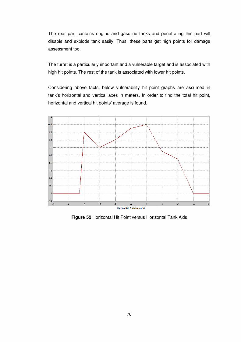
76
The rear part contains engine and gasoline tanks and penetrating this part will
disable and explode tank easily. Thus, these parts get high points for damage
assessment too.
The turret is a particularly important and a vulnerable target and is associated with
high hit points. The rest of the tank is associated with lower hit points.
Considering above facts, below vulnerability hit point graphs are assumed in
tank’s horizontal and vertical axes in meters. In order to find the total hit point,
horizontal and vertical hit points’ average is found.
Figure 52 Horizontal Hit Point versus Horizontal Tank Axis
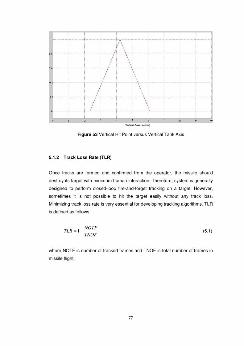
77
Figure 53 Vertical Hit Point versus Vertical Tank Axis
5.1.2 Track Loss Rate (TLR)
Once tracks are formed and confirmed from the operator, the missile should
destroy its target with minimum human interaction. Therefore, system is generally
designed to perform closed-loop fire-and-forget tracking on a target. However,
sometimes it is not possible to hit the target easily without any track loss.
Minimizing track loss rate is very essential for developing tracking algorithms. TLR
is defined as follows:
TNOF
NOTFTLR −= 1 (5.1)
where NOTF is number of tracked frames and TNOF is total number of frames in
missile flight.
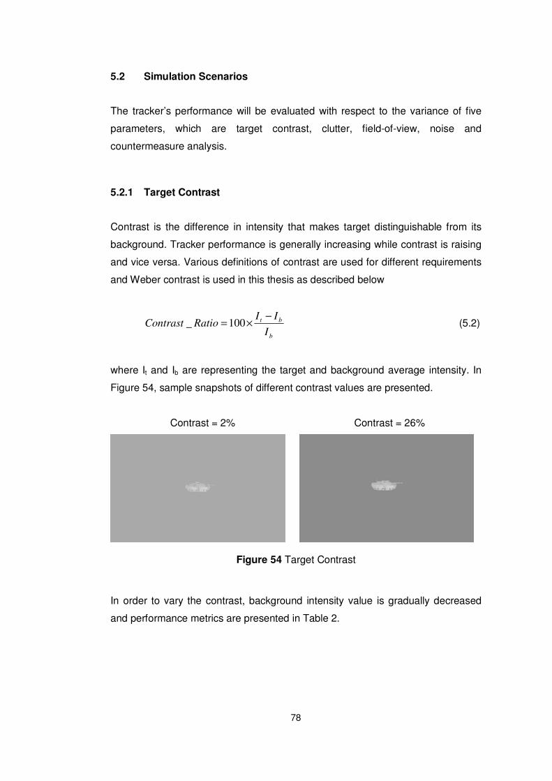
78
5.2 Simulation Scenarios
The tracker’s performance will be evaluated with respect to the variance of five
parameters, which are target contrast, clutter, field-of-view, noise and
countermeasure analysis.
5.2.1 Target Contrast
Contrast is the difference in intensity that makes target distinguishable from its
background. Tracker performance is generally increasing while contrast is raising
and vice versa. Various definitions of contrast are used for different requirements
and Weber contrast is used in this thesis as described below
b
bt
I
IIRatioContrast
−×= 100_ (5.2)
where It and Ib are representing the target and background average intensity. In
Figure 54, sample snapshots of different contrast values are presented.
Contrast = 2% Contrast = 26%
Figure 54 Target Contrast
In order to vary the contrast, background intensity value is gradually decreased
and performance metrics are presented in Table 2.
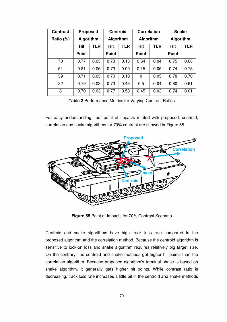
79
Contrast
Ratio (%)
Proposed
Algorithm
Centroid
Algorithm
Correlation
Algorithm
Snake
Algorithm
Hit
Point
TLR Hit
Point
TLR Hit
Point
TLR Hit
Point
TLR
70 0.77 0.03 0.73 0.13 0.64 0.04 0.75 0.68
51 0.81 0.06 0.73 0.09 0.15 0.05 0.74 0.75
39 0.71 0.03 0.70 0.18 0 0.05 0.78 0.70
22 0.79 0.03 0.73 0.43 0.5 0.04 0.80 0.61
8 0.70 0.03 0.77 0.53 0.45 0.03 0.74 0.61
Table 2 Performance Metrics for Varying Contrast Ratios
For easy understanding, four point of impacts related with proposed, centroid,
correlation and snake algorithms for 70% contrast are showed in Figure 55.
Figure 55 Point of Impacts for 70% Contrast Scenario
Centroid and snake algorithms have high track loss rate compared to the
proposed algorithm and the correlation method. Because the centroid algorithm is
sensitive to lock-on loss and snake algorithm requires relatively big target size.
On the contrary, the centroid and snake methods get higher hit points than the
correlation algorithm. Because proposed algorithm’s terminal phase is based on
snake algorithm, it generally gets higher hit points. While contrast ratio is
decreasing, track loss rate increases a little bit in the centroid and snake methods
Correlation
Snake
Centroid
Proposed
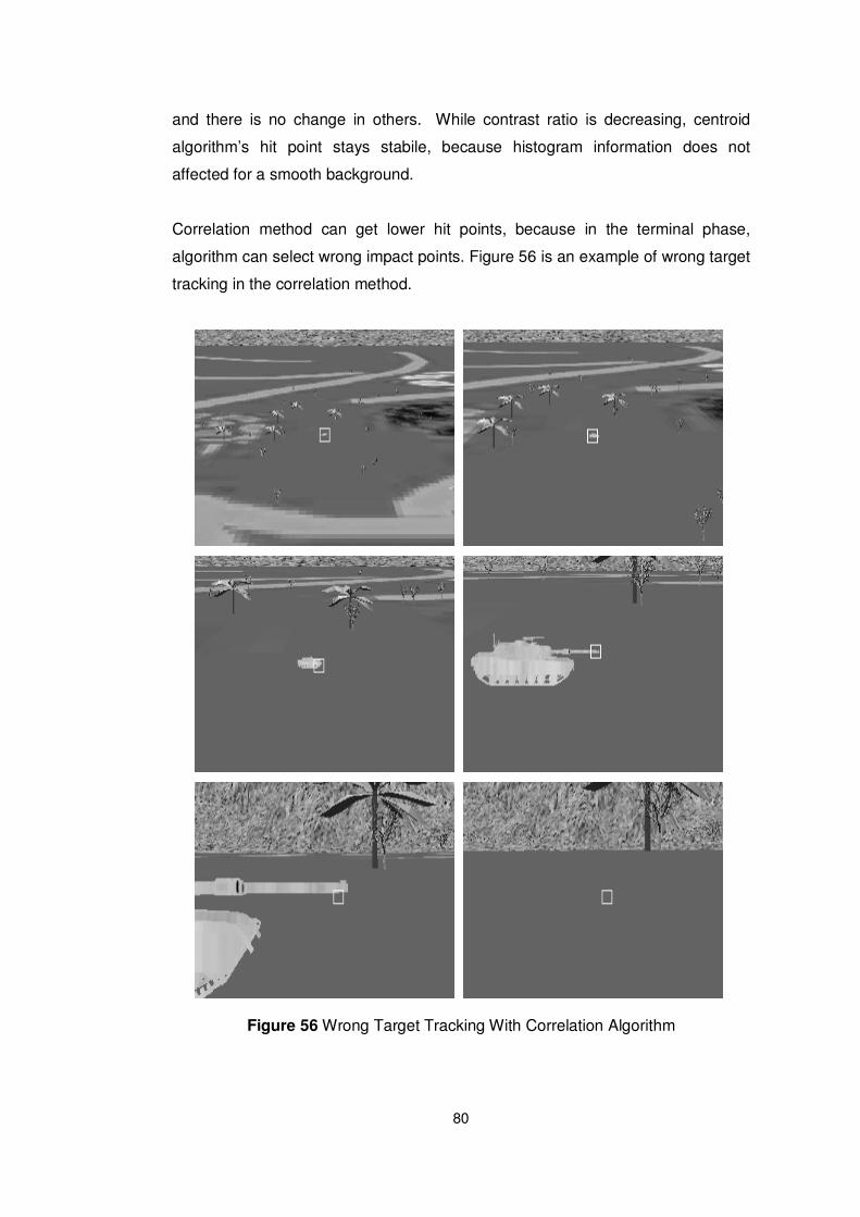
80
and there is no change in others. While contrast ratio is decreasing, centroid
algorithm’s hit point stays stabile, because histogram information does not
affected for a smooth background.
Correlation method can get lower hit points, because in the terminal phase,
algorithm can select wrong impact points. Figure 56 is an example of wrong target
tracking in the correlation method.
Figure 56 Wrong Target Tracking With Correlation Algorithm

81
5.2.2 Clutter
For imaging trackers, any object or scene phenomenon, which has significant
ability to perturb measurements, is called as clutter. A way to estimate the
influence of the clutter is to calculate statistics of the pixel distributions of the
scene.
Schemider and Weathersby suggested a measure that they called signal-to-
clutter ratio (SCR), which was defined as follows [26],
2/1
1
21
max
=
−=
∑=
N
i
i
bt
Nclutter
clutter
meanIISCR
σ
(5.3)
where maxIt is the maximum target intensity, meanIb is the mean background
intensity, σi is the standard deviation of the pixels over an area i and N is the total
divided area.
The statistics of the target and background are computed over regions defined in
Figure 57. The dimensions of the target region are one-third of the dimensions of
the background region and centered within it [27].
Figure 57 SCR Calculation Dimensions
Background
Target y
3y
3x
x
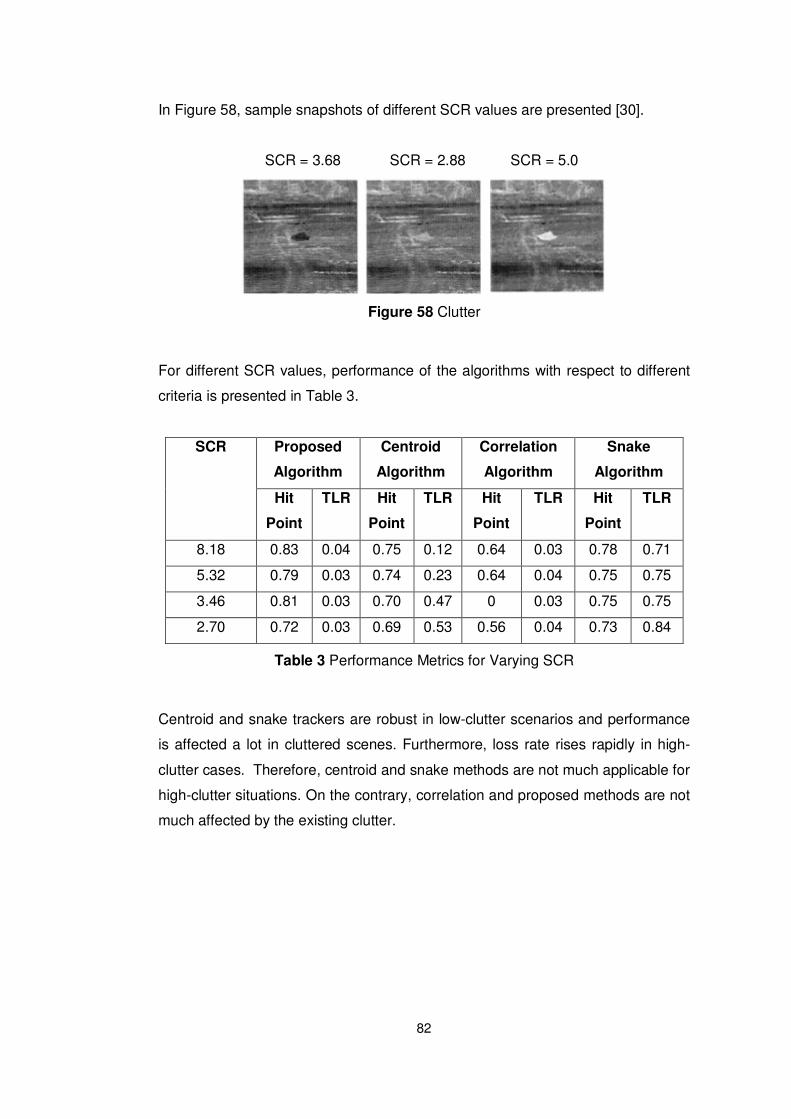
82
In Figure 58, sample snapshots of different SCR values are presented [30].
SCR = 3.68 SCR = 2.88 SCR = 5.0
Figure 58 Clutter
For different SCR values, performance of the algorithms with respect to different
criteria is presented in Table 3.
SCR Proposed
Algorithm
Centroid
Algorithm
Correlation
Algorithm
Snake
Algorithm
Hit
Point
TLR Hit
Point
TLR Hit
Point
TLR Hit
Point
TLR
8.18 0.83 0.04 0.75 0.12 0.64 0.03 0.78 0.71
5.32 0.79 0.03 0.74 0.23 0.64 0.04 0.75 0.75
3.46 0.81 0.03 0.70 0.47 0 0.03 0.75 0.75
2.70 0.72 0.03 0.69 0.53 0.56 0.04 0.73 0.84
Table 3 Performance Metrics for Varying SCR
Centroid and snake trackers are robust in low-clutter scenarios and performance
is affected a lot in cluttered scenes. Furthermore, loss rate rises rapidly in high-
clutter cases. Therefore, centroid and snake methods are not much applicable for
high-clutter situations. On the contrary, correlation and proposed methods are not
much affected by the existing clutter.
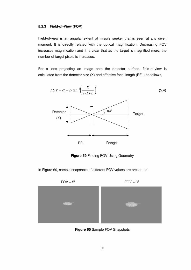
83
5.2.3 Field-of-View (FOV)
Field-of-view is an angular extent of missile seeker that is seen at any given
moment. It is directly related with the optical magnification. Decreasing FOV
increases magnification and it is clear that as the target is magnified more, the
number of target pixels is increases.
For a lens projecting an image onto the detector surface, field-of-view is
calculated from the detector size (X) and effective focal length (EFL) as follows,
⋅⋅== −
EFL
XFOV
2tan2
1α (5.4)
Figure 59 Finding FOV Using Geometry
In Figure 60, sample snapshots of different FOV values are presented.
FOV = 5º FOV = 3o
Figure 60 Sample FOV Snapshots
Detector
(X)
α/2 Target
EFL Range
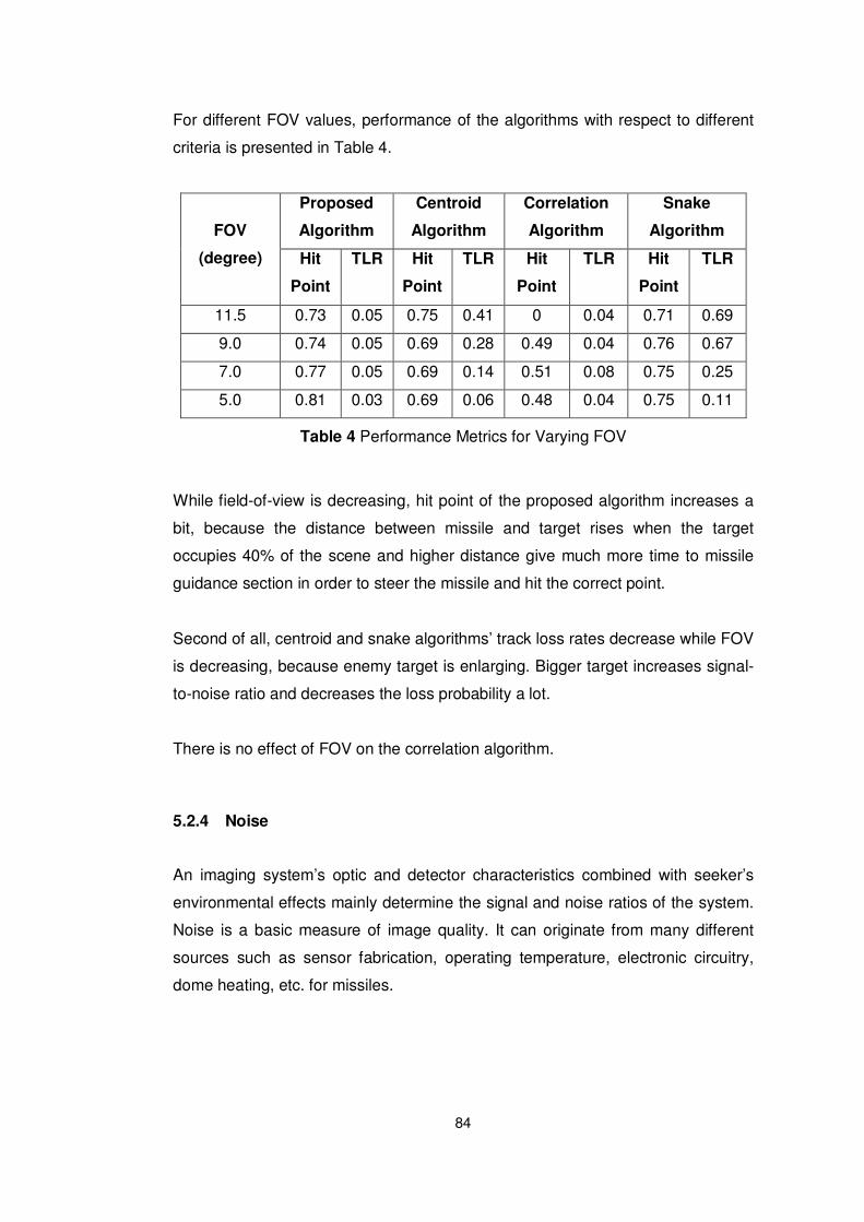
84
For different FOV values, performance of the algorithms with respect to different
criteria is presented in Table 4.
FOV
(degree)
Proposed
Algorithm
Centroid
Algorithm
Correlation
Algorithm
Snake
Algorithm
Hit
Point
TLR Hit
Point
TLR Hit
Point
TLR Hit
Point
TLR
11.5 0.73 0.05 0.75 0.41 0 0.04 0.71 0.69
9.0 0.74 0.05 0.69 0.28 0.49 0.04 0.76 0.67
7.0 0.77 0.05 0.69 0.14 0.51 0.08 0.75 0.25
5.0 0.81 0.03 0.69 0.06 0.48 0.04 0.75 0.11
Table 4 Performance Metrics for Varying FOV
While field-of-view is decreasing, hit point of the proposed algorithm increases a
bit, because the distance between missile and target rises when the target
occupies 40% of the scene and higher distance give much more time to missile
guidance section in order to steer the missile and hit the correct point.
Second of all, centroid and snake algorithms’ track loss rates decrease while FOV
is decreasing, because enemy target is enlarging. Bigger target increases signal-
to-noise ratio and decreases the loss probability a lot.
There is no effect of FOV on the correlation algorithm.
5.2.4 Noise
An imaging system’s optic and detector characteristics combined with seeker’s
environmental effects mainly determine the signal and noise ratios of the system.
Noise is a basic measure of image quality. It can originate from many different
sources such as sensor fabrication, operating temperature, electronic circuitry,
dome heating, etc. for missiles.
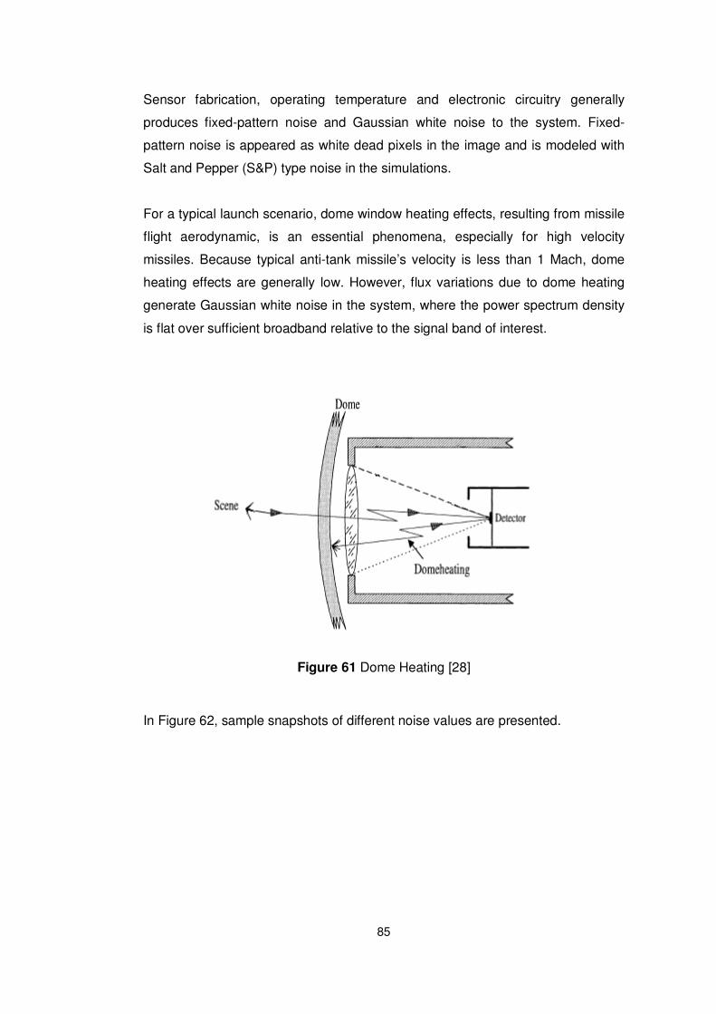
85
Sensor fabrication, operating temperature and electronic circuitry generally
produces fixed-pattern noise and Gaussian white noise to the system. Fixed-
pattern noise is appeared as white dead pixels in the image and is modeled with
Salt and Pepper (S&P) type noise in the simulations.
For a typical launch scenario, dome window heating effects, resulting from missile
flight aerodynamic, is an essential phenomena, especially for high velocity
missiles. Because typical anti-tank missile’s velocity is less than 1 Mach, dome
heating effects are generally low. However, flux variations due to dome heating
generate Gaussian white noise in the system, where the power spectrum density
is flat over sufficient broadband relative to the signal band of interest.
Figure 61 Dome Heating [28]
In Figure 62, sample snapshots of different noise values are presented.

86
%0.5 S&P %1 S&P .02 σ2 White Noise
.05 σ2 White Noise .1 σ2 White Noise
Figure 62 Sample Noise Snapshots
For different noise levels values, performance of the algorithms with respect to
different criteria is presented in Table 5.
Noise
Level
Proposed
Algorithm
Centroid
Algorithm
Correlation
Algorithm
Snake
Algorithm
Hit
Point
TLR Hit
Point
TLR Hit
Point
TLR Hit
Point
TLR
%0.5 S&P
noise
0.71 0.04 0.65 0.34 0.58 0.07 0.73 0.75
%1 S&P
noise
0.69 0.03 0.41 0.57 0.56 0.04 0.67 0.77
.02 σ2 white
noise
0.72 0.08 0.65 0.39 0.61 0.04 0.71 0.74
.05 σ2 white
noise
0.67 0.04 0.63 0.45 0.58 0.03 0.65 0.78
.1 σ2 white
noise
0.62 0.03 0.55 0.53 0.61 0.05 0.64 0.81
Table 5 Performance Metrics for Varying Noise
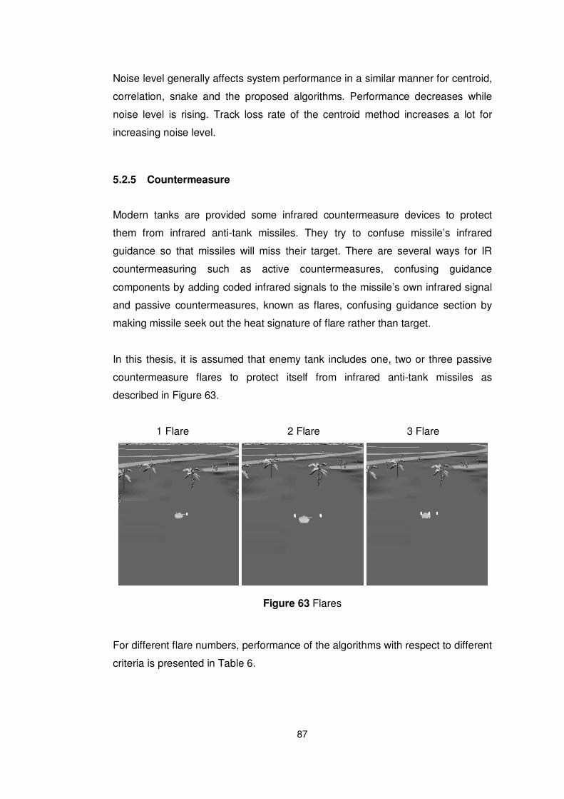
87
Noise level generally affects system performance in a similar manner for centroid,
correlation, snake and the proposed algorithms. Performance decreases while
noise level is rising. Track loss rate of the centroid method increases a lot for
increasing noise level.
5.2.5 Countermeasure
Modern tanks are provided some infrared countermeasure devices to protect
them from infrared anti-tank missiles. They try to confuse missile’s infrared
guidance so that missiles will miss their target. There are several ways for IR
countermeasuring such as active countermeasures, confusing guidance
components by adding coded infrared signals to the missile’s own infrared signal
and passive countermeasures, known as flares, confusing guidance section by
making missile seek out the heat signature of flare rather than target.
In this thesis, it is assumed that enemy tank includes one, two or three passive
countermeasure flares to protect itself from infrared anti-tank missiles as
described in Figure 63.
1 Flare 2 Flare 3 Flare
Figure 63 Flares
For different flare numbers, performance of the algorithms with respect to different
criteria is presented in Table 6.
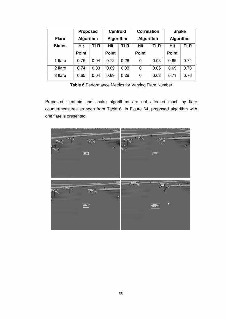
88
Flare
States
Proposed
Algorithm
Centroid
Algorithm
Correlation
Algorithm
Snake
Algorithm
Hit
Point
TLR Hit
Point
TLR Hit
Point
TLR Hit
Point
TLR
1 flare 0.76 0.04 0.72 0.28 0 0.03 0.69 0.74
2 flare 0.74 0.03 0.69 0.33 0 0.05 0.69 0.73
3 flare 0.65 0.04 0.69 0.29 0 0.03 0.71 0.76
Table 6 Performance Metrics for Varying Flare Number
Proposed, centroid and snake algorithms are not affected much by flare
countermeasures as seen from Table 6. In Figure 64, proposed algorithm with
one flare is presented.
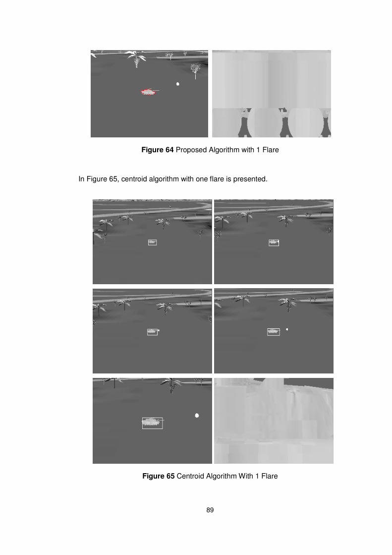
89
Figure 64 Proposed Algorithm with 1 Flare
In Figure 65, centroid algorithm with one flare is presented.
Figure 65 Centroid Algorithm With 1 Flare
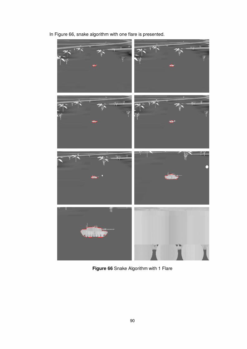
90
In Figure 66, snake algorithm with one flare is presented.
Figure 66 Snake Algorithm with 1 Flare
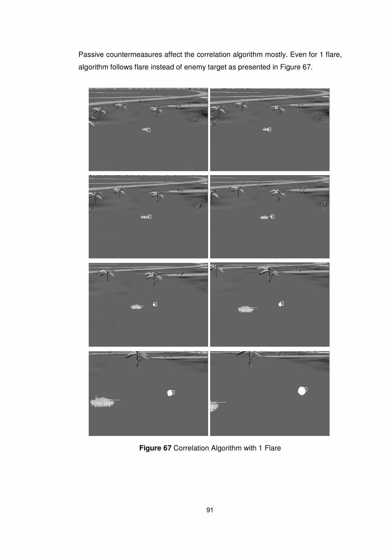
91
Passive countermeasures affect the correlation algorithm mostly. Even for 1 flare,
algorithm follows flare instead of enemy target as presented in Figure 67.
Figure 67 Correlation Algorithm with 1 Flare
92
CHAPTER 6
6 CONCLUSION
In this study, two autopilot control schemes (PID and LQR) are developed for an
anti-tank missile after constructing their mathematical models. PID control
technique is selected for the rest of the work, because it satisfies all of the
requirements. Inputs for the autopilot section are considered as target and missile
error angle.
A typical imaging infrared seeker model is constructed with its subcomponents
imager, gimbal and processor. Generating infrared imaging scene concept is
presented. Two-axis and stabilized gimbal structure is developed. Three tracking
algorithms such as centroid, correlation and active contour (snake) are
considered for the processor section. Then, a new proposed tracking algorithm
combining these methods in order to improve kill rate is developed.
Virtual simulation studies are carried out in order to present the effectiveness of
proposed tracking algorithm comparing with centroid, correlation and snake
algorithms for different test scenarios. This study shows that proposed tracking
algorithm increases the hit and kill rate in different scenarios. There are many
advantageous of the proposed algorithm, especially in high-clutter and noisy real-
world environments. Even when the target tank has one, two or three passive
countermeasure flares to protect itself from infrared anti-tank missiles, proposed
algorithm can hit and destroy its enemy with higher probability.
As a future work, tracking algorithm could be improved by combining effective
filtering blocks such as Kalman Filter. It provides an efficient recursive
computational estimate of the state of the process, which improves tracking

93
capability by predicting future states. Second of all, proportional guidance instead
of pursuit guidance could be developed in order to destroy moving enemy targets
effectively. Target’s mathematical model could be implemented as well.
Commercial infrared scene generators could be integrated to the work. It
increases the ability to simulate infrared scenes more effectively and comparing
different wavelengths such as MWIR and LWIR could be possible.
94
REFERENCES
[1] Terry, A. F., “Short-Range Surface-To-Surface Missile Guidance for Nonlinear
Time-Varying Target State Estimation and Missile Dynamics”, Ph.D. Thesis,
Texas University, 1995.
[2] Nasburg, R.E., “Tracking and Control Systems”, Hughes Aircraft Company,
1994.
[3] Hilkert, J. M., “Stabilization, Pointing and Tracking System Technology
Handbook”, Texas Instruments, 1991.
[4] Zarchan, P., “Tactical and Strategic Missile Guidance”, American Institute of
Aeronautics and Astronautics Inc., USA, 1994.
[5] McLean D., “Automatic Flight Control Systems”, Prentice Hall International,
1990.
[6] Boiffier J., “The Dynamics of Flight the Equations”, John Wiley&Sons, 1997.
[7] Fossen T., “Guidance and Control of Ocean Vehicles” John Wiley&Sons,
1994.
[8] Ateşoğlu, Ö., “Different Autopilot Designs and Their Performance Comparison
for Guided Missiles”, Master’s Thesis, METU, 1996.
[9] Evcimen, Ç., “Development and Comparison of Autopilots and Guidance
Algorithms for Missiles”, Master’s Thesis, METU, 2007.

95
[10] Paz A. Robert, “The Design of the PID Controller”, Klipsch School of
Electrical and Computer Engineering, 2001.
[11] Dorf C. Richard, Bishop H. Robert,“Modern Control Systems“, Prentice Hall,
2001.
[12] Karasu, Ç., “Small Size Unmanned Model Helicopter Guidance and Control”,
Master’s Thesis, METU, 2004.
[13] Burns Keith A. and Blake William B. Blake, “Missile DATCOM User’s
Manual”, 1993.
[14] Holst, G. C., “Electro-optical Imaging Systems Performance”, JCD Publishing,
2000.
[15] Fischer R. E., Tadic-Galeb B., Yoder P. R., “Optical System Design”,
McGraw-Hill Books, 2008.
[16] Vollmerhausen R., “Predicting Field Target Acquisition Performance”, US
Army Night Vision and Electronic Sensors Directorate, 2002.
[17] Brackney B. A., Hammon R. K., Hall R. L., Phillips M. A., “Development of
Simulation Tools for the Analysis of Captive Flight Test Data for Imaging Infrared
Missile Seekers”, Proceedings of SPIE, pp.26-33, 2001.
[18] Çolakoğlu, Ç. “Performance Evaluation of Video Trackers Using Synthetic
Scenarios”, Master’s Thesis, METU, 1999.
[19] MATLAB Virtual Reality Toolbox User’s Guide, Mathworks, 2004.
[20] "HSL and HSV" Wikipedia, The Free Encyclopedia. 26 Jul 2008, 18:09 UTC.
Wikimedia Foundation, Inc., 27 Jul 2008
<http://en.wikipedia.org/w/index.php?title=HSL_and_HSV&oldid=228043437>.

96
[21] Blakelock J. H., “Automatic Control of Aircraft and Missiles”, John Wiley &
Sons Inc., 1991.
[22] Blackman S., Popoli R., “Design and Analysis of Modern Tracking Systems”,
Artech House, 1999.
[23] Venkateswarlu R., Sujata K. V., Rao B. V., “Centroid Tracker and Aim Point
Selection”, SPIE Vol. 1697 Acquisition, Tracking and Pointing VI, pp.520-529,
1992.
[24] “VRealm Builder User’s Guide and Reference”, Ligos Corporation, 1997.
[25] “Tactical and Technical Trends: Vulnerability of Tiger Tanks”, US Military
Intelligence Service, Section 1, 1943.
[26] Schmieder D. A., Weathersby M. R., “Detection Performance In Clutter With
Variable Resolution”, IEEE Trans. Aerop. Electron. Syst., Vol. AES-19, No.3,
pp.622-630, 1983.
[27] Scott A. N., Naylor R. B., “Reliable Motion Detection of Small Targets in
Video With Low Signal-to-Clutter Ratios”, IEEE Trans., pp.447-456, 1995.
[28] Naveh O., “Sensitivity of Scanning and Staring IR Seekers for Air-to-Air
Missiles”, Proceedings of SPIE, pp.692-711, 1997.
[29] "MCLOS" Wikipedia, The Free Encyclopedia. 8 Aug 2008, 17:48 UTC.
Wikimedia Foundation, Inc. 12 Aug 2008
<http://en.wikipedia.org/w/index.php?title=MCLOS&oldid=230653996>.
[30] Phillips M. A., Sims S. R. F., “A Signal to Clutter Measure for ATR
Performance Comparison”, Proceedings of SPIE, pp.74-81, 1997.
[31] Hamarneh G., “Towards Intelligent Deformable Models for Medical Image
Analysis”, Ph.D. Thesis, Chalmers University of Technology, 2001.

97
[32] Kass M., Witkin A., Terzopoulos D., “Snakes: Active contour models”
International Journal of Computer Vision, 1988.
[33] F. L. Kok, “Deformable Contours: Modeling, Extraction, Detection, and
Classification” Ph.D. Thesis, University of Wisconsin-Madison, 1994.

98
APPENDIX A
MISSILE DATCOM USER MANUAL
The fundamental purpose of the Missile DATCOM software is to provide an
aerodynamic design and the capability for the user to easily substitute methods to
fit specific applications [13].
A.1. Input Definitions
The user can enter the flight conditions and geometry of the desired missile using
variety of namelist inputs and control cards. These data should be written in
“for005.dat” file.
A.2. Namelist Inputs
Flight conditions, reference quantities, axisymmetric body definitions, etc. briefly
all properties of desired missile are provided by ten namelists. These namelists
are summarized as follows:
Namelist Definition
FLTCON Flight conditions (angle of attack, Mach numbers, etc.)
REFQ Reference quantities (reference area, length, etc.)
AXIBOD Axisymmetric body definitions
ELLBOD Elliptical body definitions
PROTUB Protuberance information and geometry
FINSETn Fin descriptions by fin set (n is the fin set number 1,2,3
or 4)
DEFLCT Panel deflection values
TRIM Trimming information

99
INLET Inlet geometry
EXPR Experimental data
Table 7 Namelist Inputs
The following rules are common for all namelists:
• Namelist parts start with symbol “$” and ends with the same symbol.
• The namelist can be input any order.
• Namelist inputs are column independent and can begin in any column
including the 1st. If a namelist is continued to a second card, the continued
card must leave column 1 blank. Also, the card before the continued card
must end with a comma. The last usable column is number 79 if column 1
is used and column 80 if column 1 is blank.
• The same namelist can be input multiple times for the same input case.
The total number of namelists read, including repeat occurrences of the
same namelist name, must not exceed 300.
• The last occurrence of a namelist variable in a case is the value for the
calculations.
In our configuration, FLTCON, REFQ, AXIBOD, FINSETn, DEFLCT and TRIM
namelists are provided to the software as follows:
A.3. Flight Conditions
In order to define the flight conditions FLTCON namelist should be run. The
program is limited to no more than 20 angle of attack and 20 Mach numbers.
Therefore, a case is defined as a 10 Mach numbers and 20 angles of attacks as
follows:
$FLTCON
NMACH= 10.0,NALPHA= 20.0,ALT= 0.0,
MACH(1)=.1,.2,.3,.4,.5,.6,.7,.8,.9,1.0,
ALPHA(1)=-9.,-8.,-7.,-6.,-5.,-4.,-3.,-2.,-1.,0.0,
ALPHA(11)=1.,2.,3.,4.,5.,6.,7.,8.,9.,10.,
BETA=0.0,
$END
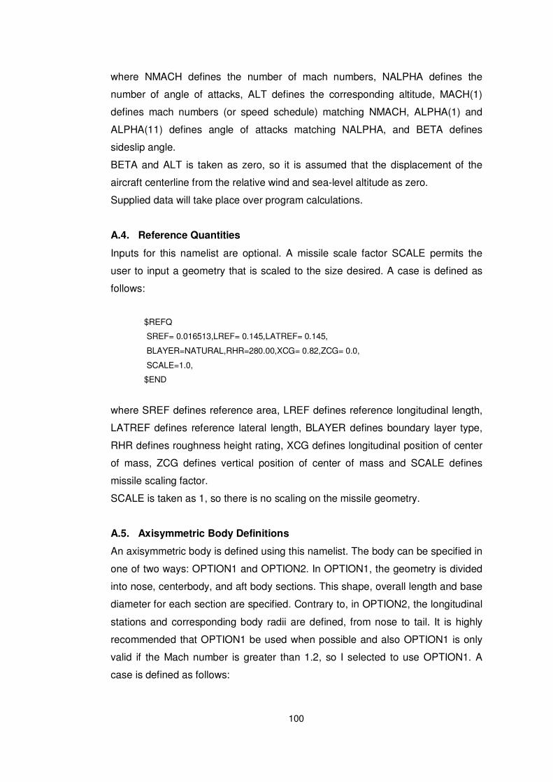
100
where NMACH defines the number of mach numbers, NALPHA defines the
number of angle of attacks, ALT defines the corresponding altitude, MACH(1)
defines mach numbers (or speed schedule) matching NMACH, ALPHA(1) and
ALPHA(11) defines angle of attacks matching NALPHA, and BETA defines
sideslip angle.
BETA and ALT is taken as zero, so it is assumed that the displacement of the
aircraft centerline from the relative wind and sea-level altitude as zero.
Supplied data will take place over program calculations.
A.4. Reference Quantities
Inputs for this namelist are optional. A missile scale factor SCALE permits the
user to input a geometry that is scaled to the size desired. A case is defined as
follows:
$REFQ
SREF= 0.016513,LREF= 0.145,LATREF= 0.145,
BLAYER=NATURAL,RHR=280.00,XCG= 0.82,ZCG= 0.0,
SCALE=1.0,
$END
where SREF defines reference area, LREF defines reference longitudinal length,
LATREF defines reference lateral length, BLAYER defines boundary layer type,
RHR defines roughness height rating, XCG defines longitudinal position of center
of mass, ZCG defines vertical position of center of mass and SCALE defines
missile scaling factor.
SCALE is taken as 1, so there is no scaling on the missile geometry.
A.5. Axisymmetric Body Definitions
An axisymmetric body is defined using this namelist. The body can be specified in
one of two ways: OPTION1 and OPTION2. In OPTION1, the geometry is divided
into nose, centerbody, and aft body sections. This shape, overall length and base
diameter for each section are specified. Contrary to, in OPTION2, the longitudinal
stations and corresponding body radii are defined, from nose to tail. It is highly
recommended that OPTION1 be used when possible and also OPTION1 is only
valid if the Mach number is greater than 1.2, so I selected to use OPTION1. A
case is defined as follows:
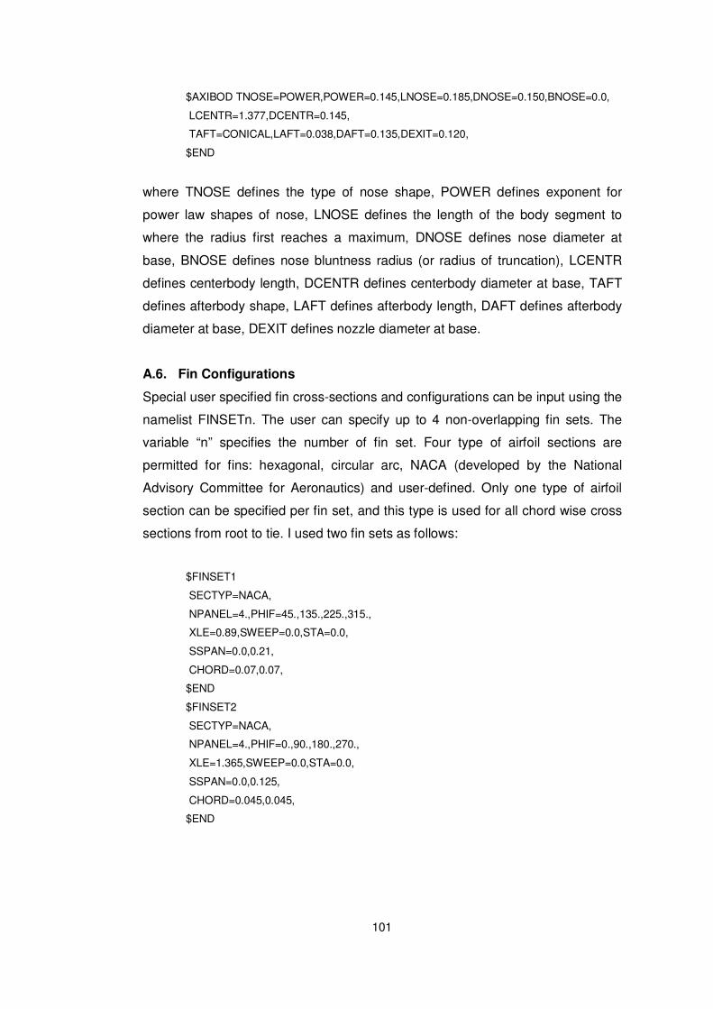
101
$AXIBOD TNOSE=POWER,POWER=0.145,LNOSE=0.185,DNOSE=0.150,BNOSE=0.0,
LCENTR=1.377,DCENTR=0.145,
TAFT=CONICAL,LAFT=0.038,DAFT=0.135,DEXIT=0.120,
$END
where TNOSE defines the type of nose shape, POWER defines exponent for
power law shapes of nose, LNOSE defines the length of the body segment to
where the radius first reaches a maximum, DNOSE defines nose diameter at
base, BNOSE defines nose bluntness radius (or radius of truncation), LCENTR
defines centerbody length, DCENTR defines centerbody diameter at base, TAFT
defines afterbody shape, LAFT defines afterbody length, DAFT defines afterbody
diameter at base, DEXIT defines nozzle diameter at base.
A.6. Fin Configurations
Special user specified fin cross-sections and configurations can be input using the
namelist FINSETn. The user can specify up to 4 non-overlapping fin sets. The
variable “n” specifies the number of fin set. Four type of airfoil sections are
permitted for fins: hexagonal, circular arc, NACA (developed by the National
Advisory Committee for Aeronautics) and user-defined. Only one type of airfoil
section can be specified per fin set, and this type is used for all chord wise cross
sections from root to tie. I used two fin sets as follows:
$FINSET1
SECTYP=NACA,
NPANEL=4.,PHIF=45.,135.,225.,315.,
XLE=0.89,SWEEP=0.0,STA=0.0,
SSPAN=0.0,0.21,
CHORD=0.07,0.07,
$END
$FINSET2
SECTYP=NACA,
NPANEL=4.,PHIF=0.,90.,180.,270.,
XLE=1.365,SWEEP=0.0,STA=0.0,
SSPAN=0.0,0.125,
CHORD=0.045,0.045,
$END
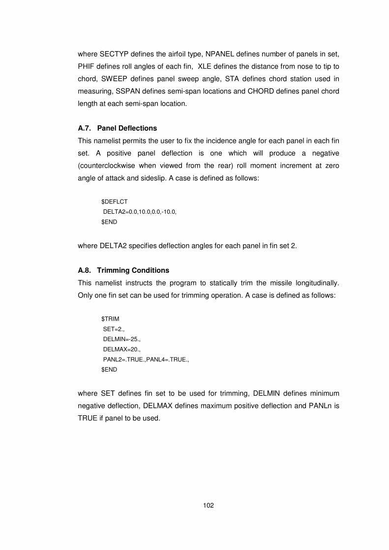
102
where SECTYP defines the airfoil type, NPANEL defines number of panels in set,
PHIF defines roll angles of each fin, XLE defines the distance from nose to tip to
chord, SWEEP defines panel sweep angle, STA defines chord station used in
measuring, SSPAN defines semi-span locations and CHORD defines panel chord
length at each semi-span location.
A.7. Panel Deflections
This namelist permits the user to fix the incidence angle for each panel in each fin
set. A positive panel deflection is one which will produce a negative
(counterclockwise when viewed from the rear) roll moment increment at zero
angle of attack and sideslip. A case is defined as follows:
$DEFLCT
DELTA2=0.0,10.0,0.0,-10.0,
$END
where DELTA2 specifies deflection angles for each panel in fin set 2.
A.8. Trimming Conditions
This namelist instructs the program to statically trim the missile longitudinally.
Only one fin set can be used for trimming operation. A case is defined as follows:
$TRIM
SET=2.,
DELMIN=-25.,
DELMAX=20.,
PANL2=.TRUE.,PANL4=.TRUE.,
$END
where SET defines fin set to be used for trimming, DELMIN defines minimum
negative deflection, DELMAX defines maximum positive deflection and PANLn is
TRUE if panel to be used.
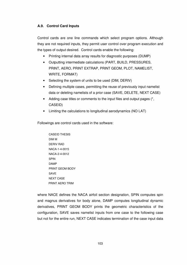
103
A.9. Control Card Inputs
Control cards are one line commands which select program options. Although
they are not required inputs, they permit user control over program execution and
the types of output desired. Control cards enable the following:
• Printing internal data array results for diagnostic purposes (DUMP)
• Outputting intermediate calculations (PART, BUILD, PRESSURES,
PRINT, AERO, PRINT EXTRAP, PRINT GEOM, PLOT, NAMELIST,
WRITE, FORMAT)
• Selecting the system of units to be used (DIM, DERIV)
• Defining multiple cases, permitting the reuse of previously input namelist
data or deleting namelists of a prior case (SAVE, DELETE, NEXT CASE)
• Adding case titles or comments to the input files and output pages (*,
CASEID)
• Limiting the calculations to longitudinal aerodynamics (NO LAT)
Followings are control cards used in the software:
CASEID THESIS
DIM M
DERIV RAD
NACA-1-4-0015
NACA-2-4-0012
SPIN
DAMP
PRINT GEOM BODY
SAVE
NEXT CASE
PRINT AERO TRIM
where NACE defines the NACA airfoil section designation, SPIN computes spin
and magnus derivatives for body alone, DAMP computes longitudinal dynamic
derivatives, PRINT GEOM BODY prints the geometric characteristics of the
configuration, SAVE saves namelist inputs from one case to the following case
but not for the entire run, NEXT CASE indicates termination of the case input data
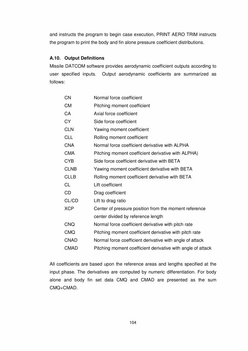
104
and instructs the program to begin case execution, PRINT AERO TRIM instructs
the program to print the body and fin alone pressure coefficient distributions.
A.10. Output Definitions
Missile DATCOM software provides aerodynamic coefficient outputs according to
user specified inputs. Output aerodynamic coefficients are summarized as
follows:
CN Normal force coefficient
CM Pitching moment coefficient
CA Axial force coefficient
CY Side force coefficient
CLN Yawing moment coefficient
CLL Rolling moment coefficient
CNA Normal force coefficient derivative with ALPHA
CMA Pitching moment coefficient derivative with ALPHA)
CYB Side force coefficient derivative with BETA
CLNB Yawing moment coefficient derivative with BETA
CLLB Rolling moment coefficient derivative with BETA
CL Lift coefficient
CD Drag coefficient
CL/CD Lift to drag ratio
XCP Center of pressure position from the moment reference
center divided by reference length
CNQ Normal force coefficient derivative with pitch rate
CMQ Pitching moment coefficient derivative with pitch rate
CNAD Normal force coefficient derivative with angle of attack
CMAD Pitching moment coefficient derivative with angle of attack
All coefficients are based upon the reference areas and lengths specified at the
input phase. The derivatives are computed by numeric differentiation. For body
alone and body fin set data CMQ and CMAD are presented as the sum
CMQ+CMAD.
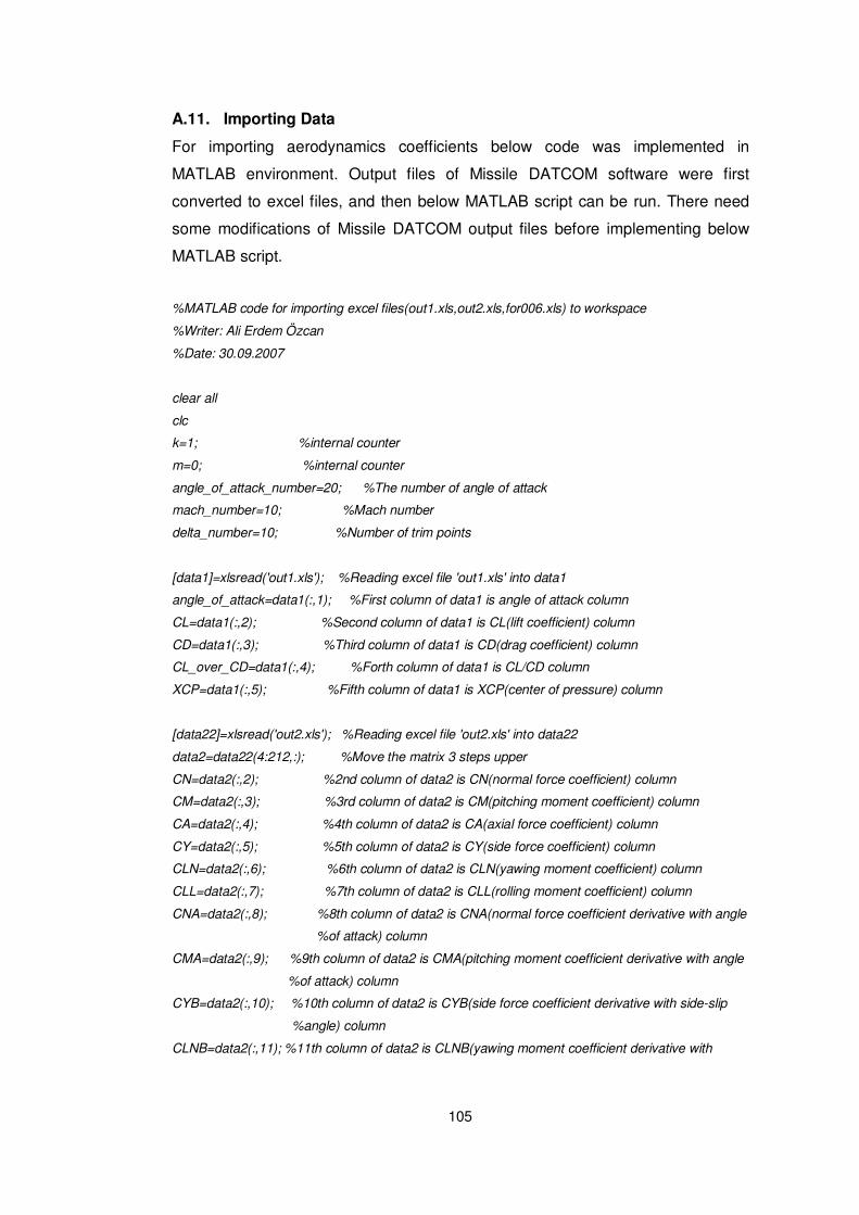
105
A.11. Importing Data
For importing aerodynamics coefficients below code was implemented in
MATLAB environment. Output files of Missile DATCOM software were first
converted to excel files, and then below MATLAB script can be run. There need
some modifications of Missile DATCOM output files before implementing below
MATLAB script.
%MATLAB code for importing excel files(out1.xls,out2.xls,for006.xls) to workspace
%Writer: Ali Erdem Özcan
%Date: 30.09.2007
clear all
clc
k=1; %internal counter
m=0; %internal counter
angle_of_attack_number=20; %The number of angle of attack
mach_number=10; %Mach number
delta_number=10; %Number of trim points
[data1]=xlsread('out1.xls'); %Reading excel file 'out1.xls' into data1
angle_of_attack=data1(:,1); %First column of data1 is angle of attack column
CL=data1(:,2); %Second column of data1 is CL(lift coefficient) column
CD=data1(:,3); %Third column of data1 is CD(drag coefficient) column
CL_over_CD=data1(:,4); %Forth column of data1 is CL/CD column
XCP=data1(:,5); %Fifth column of data1 is XCP(center of pressure) column
[data22]=xlsread('out2.xls'); %Reading excel file 'out2.xls' into data22
data2=data22(4:212,:); %Move the matrix 3 steps upper
CN=data2(:,2); %2nd column of data2 is CN(normal force coefficient) column
CM=data2(:,3); %3rd column of data2 is CM(pitching moment coefficient) column
CA=data2(:,4); %4th column of data2 is CA(axial force coefficient) column
CY=data2(:,5); %5th column of data2 is CY(side force coefficient) column
CLN=data2(:,6); %6th column of data2 is CLN(yawing moment coefficient) column
CLL=data2(:,7); %7th column of data2 is CLL(rolling moment coefficient) column
CNA=data2(:,8); %8th column of data2 is CNA(normal force coefficient derivative with angle
%of attack) column
CMA=data2(:,9); %9th column of data2 is CMA(pitching moment coefficient derivative with angle
%of attack) column
CYB=data2(:,10); %10th column of data2 is CYB(side force coefficient derivative with side-slip
%angle) column
CLNB=data2(:,11); %11th column of data2 is CLNB(yawing moment coefficient derivative with

106
%sideslip angle) column
CLLB=data2(:,11); %12th column of data2 is CLLB(rolling moment coefficient derivative with side-
%slip angle) column
[data3]=xlsread('for006.xls'); %Reading excel file 'for006.xls' into data3
[row_data3,column_data3]=size(data3);
for m=0:(mach_number-1)
CNQ((angle_of_attack_number*m+1):(angle_of_attack_number*m+angle_of_attack_number))=data
3(((103*m+234):(103*m+253)),6);
CNAD((angle_of_attack_number*m+1):(angle_of_attack_number*m+angle_of_attack_number))=dat
a3(((103*m+234):(103*m+253)),8);
CMQ_CMAD((angle_of_attack_number*m+1):(angle_of_attack_number*m+angle_of_attack_numbe
r))=data3(((103*m+234):(103*m+253)),9)*100;
end
CNQ=CNQ'; %Takes its transpose in order to make CNQ as 200x1
CNAD=CNAD'; %Takes its transpose in order to make CNAD as 200x1
CMQ_CMAD=CMQ_CMAD'; %Takes its transpose in order to make CMQ+CMAD as 200x1
CMQ_CMAD(141,1)=CMQ_CMAD(141,1)/10; %Modification should be necessary
CMQ_CMAD(159,1)=CMQ_CMAD(159,1)/10; %Modification should be necessary
CMQ_CMAD(160,1)=CMQ_CMAD(160,1)/10; %Modification should be necessary
CMQ_CMAD(161,1)=CMQ_CMAD(161,1)/10; %Modification should be necessary
CMQ_CMAD(179,1)=CMQ_CMAD(179,1)/10; %Modification should be necessary
CMQ_CMAD(180,1)=CMQ_CMAD(180,1)/10; %Modification should be necessary
for m=0:9
for j=1:6
Delta_neg_25(((120*m)+((j-1)*20)+1):((120*m)+((j-1)*20)+20)) = data3(((43*(j-
1)+1218+(m*317)):(43*(j-1)+1237+(m*317))),3); %-25 degree panel deflection
Delta_neg_20(((120*m)+((j-1)*20)+1):((120*m)+((j-1)*20)+20)) = data3(((43*(j-
1)+1218+(m*317)):(43*(j-1)+1237+(m*317))),4); %-20 degree panel deflection
Delta_neg_15(((120*m)+((j-1)*20)+1):((120*m)+((j-1)*20)+20)) = data3(((43*(j-
1)+1218+(m*317)):(43*(j-1)+1237+(m*317))),5); %-15 degree panel deflection
Delta_neg_10(((120*m)+((j-1)*20)+1):((120*m)+((j-1)*20)+20)) = data3(((43*(j-
1)+1218+(m*317)):(43*(j-1)+1237+(m*317))),6); %-10 degree panel deflection
Delta_neg_05(((120*m)+((j-1)*20)+1):((120*m)+((j-1)*20)+20)) = data3(((43*(j-
1)+1218+(m*317)):(43*(j-1)+1237+(m*317))),7); %-5 degree panel deflection
107
Delta_0(((120*m)+((j-1)*20)+1):((120*m)+((j-1)*20)+20)) = data3(((43*(j-
1)+1218+(m*317)):(43*(j-1)+1237+(m*317))),8); %0 degree panel deflection
Delta_pos_05(((120*m)+((j-1)*20)+1):((120*m)+((j-1)*20)+20)) = data3(((43*(j-
1)+1218+(m*317)):(43*(j-1)+1237+(m*317))),9); %5 degree panel deflection
Delta_pos_10(((120*m)+((j-1)*20)+1):((120*m)+((j-1)*20)+20)) = data3(((43*(j-
1)+1218+(m*317)):(43*(j-1)+1237+(m*317))),10);%10 degree panel deflection
Delta_pos_15(((120*m)+((j-1)*20)+1):((120*m)+((j-1)*20)+20)) = data3(((43*(j-
1)+1218+(m*317)):(43*(j-1)+1237+(m*317))),11);%15 degree panel deflection
Delta_pos_20(((120*m)+((j-1)*20)+1):((120*m)+((j-1)*20)+20)) = data3(((43*(j-
1)+1218+(m*317)):(43*(j-1)+1237+(m*317))),12);%20 degree panel deflection
end
end
Delta_neg_25=Delta_neg_25'; %Make them column vector
Delta_neg_20=Delta_neg_20';
Delta_neg_15=Delta_neg_15';
Delta_neg_10=Delta_neg_10';
Delta_neg_05=Delta_neg_05';
Delta_0=Delta_0';
Delta_pos_05=Delta_pos_05';
Delta_pos_10=Delta_pos_10';
Delta_pos_15=Delta_pos_15';
Delta_pos_20=Delta_pos_20';
% not to care NaN elements of parameters
[row,column]=size(angle_of_attack);
for i=1:row
if mod(i,(angle_of_attack_number+1))~=0
if ~isnan(angle_of_attack(i,1))
angle_of_attack_modified(k,1)=angle_of_attack(i,1);
else
angle_of_attack_modified(k,1)=0;
end
if ~isnan(CL(i,1))
CL_modified(k,1)=CL(i,1);
else
CL_modified(k,1)=0;
end
if ~isnan(CD(i,1))
CD_modified(k,1)=CD(i,1);
else
108
CD_modified(k,1)=0;
end
if ~isnan(CL_over_CD(i,1))
CL_over_CD_modified(k,1)=CL_over_CD(i,1);
else
CL_over_CD_modified(k,1)=0;
end
if ~isnan(XCP(i,1))
XCP_modified(k,1)=XCP(i,1);
else
XCP_modified(k,1)=0;
end
if ~isnan(CN(i,1))
CN_modified(k,1)=CN(i,1);
else
CN_modified(k,1)=0;
end
if ~isnan(CM(i,1))
CM_modified(k,1)=CM(i,1);
else
CM_modified(k,1)=0;
end
if ~isnan(CA(i,1))
CA_modified(k,1)=CA(i,1);
else
CA_modified(k,1)=0;
end
if ~isnan(CY(i,1))
CY_modified(k,1)=CY(i,1);
else
CY_modified(k,1)=0;
end
if ~isnan(CLN(i,1))
CLN_modified(k,1)=CLN(i,1);
else
109
CLN_modified(k,1)=0;
end
if ~isnan(CLL(i,1))
CLL_modified(k,1)=CLL(i,1);
else
CLL_modified(k,1)=0;
end
if ~isnan(CNA(i,1))
CNA_modified(k,1)=CNA(i,1);
else
CNA_modified(k,1)=0;
end
if ~isnan(CMA(i,1))
CMA_modified(k,1)=CMA(i,1);
else
CMA_modified(k,1)=0;
end
if ~isnan(CYB(i,1))
CYB_modified(k,1)=CYB(i,1);
else
CYB_modified(k,1)=0;
end
if ~isnan(CLNB(i,1))
CLNB_modified(k,1)=CLNB(i,1);
else
CLNB_modified(k,1)=0;
end
if ~isnan(CLLB(i,1))
CLLB_modified(k,1)=CLLB(i,1);
else
CLLB_modified(k,1)=0;
end
k=k+1;
end
end
110
APPENDIX B
VIRTUAL REALITY TOOLBOX USER MANUAL
The fundamental purpose of the Virtual Reality Toolbox software is to provide a
connection between a virtual world to Simulink and MATLAB® [19]. It provides a
solution for viewing and interacting with dynamic systems in a 3D virtual reality
environment. To provide a complete working environment, the Virtual Reality
Toolbox includes the following components:
• VRML editor: A classical VRML authoring tool, VRealm Builder, is
included.
• VRML viewer: It visualizes and explores virtual world created by VRML
editor.
B.1. VRML Overview
The Virtual Reality Modeling Language (VRML) is the language to display 3D
objects with a VRML viewer. Since people started to publish their documents on
the World Wide Web, there has been an effort to enhance the content of web
pages with a 3D graphics. In 1994, a Virtual Reality Markup Language was first
introduced as a 3D web standard. Soon afterward, the name for standards
became Virtual Reality Modeling Language (VRML). The result of the effort was to
produce the VRML1 specification. The VRML1 standard was implemented in
several VRML browsers, but it only allowed static virtual worlds. Quickly a new
robust extension of VRML1 was published as VRML2, which includes 3D
animation capabilities. In 1997, it was adopted as International Standard ISO/IEC
14772-1:1997 [19]. Since then it is referred as VRML97. The VRML97 standard
continues to be improved.
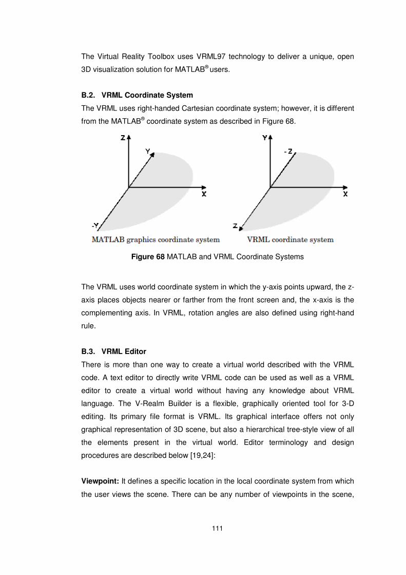
111
The Virtual Reality Toolbox uses VRML97 technology to deliver a unique, open
3D visualization solution for MATLAB® users.
B.2. VRML Coordinate System
The VRML uses right-handed Cartesian coordinate system; however, it is different
from the MATLAB® coordinate system as described in Figure 68.
Figure 68 MATLAB and VRML Coordinate Systems
The VRML uses world coordinate system in which the y-axis points upward, the z-
axis places objects nearer or farther from the front screen and, the x-axis is the
complementing axis. In VRML, rotation angles are also defined using right-hand
rule.
B.3. VRML Editor
There is more than one way to create a virtual world described with the VRML
code. A text editor to directly write VRML code can be used as well as a VRML
editor to create a virtual world without having any knowledge about VRML
language. The V-Realm Builder is a flexible, graphically oriented tool for 3-D
editing. Its primary file format is VRML. Its graphical interface offers not only
graphical representation of 3D scene, but also a hierarchical tree-style view of all
the elements present in the virtual world. Editor terminology and design
procedures are described below [19,24]:
Viewpoint: It defines a specific location in the local coordinate system from which
the user views the scene. There can be any number of viewpoints in the scene,
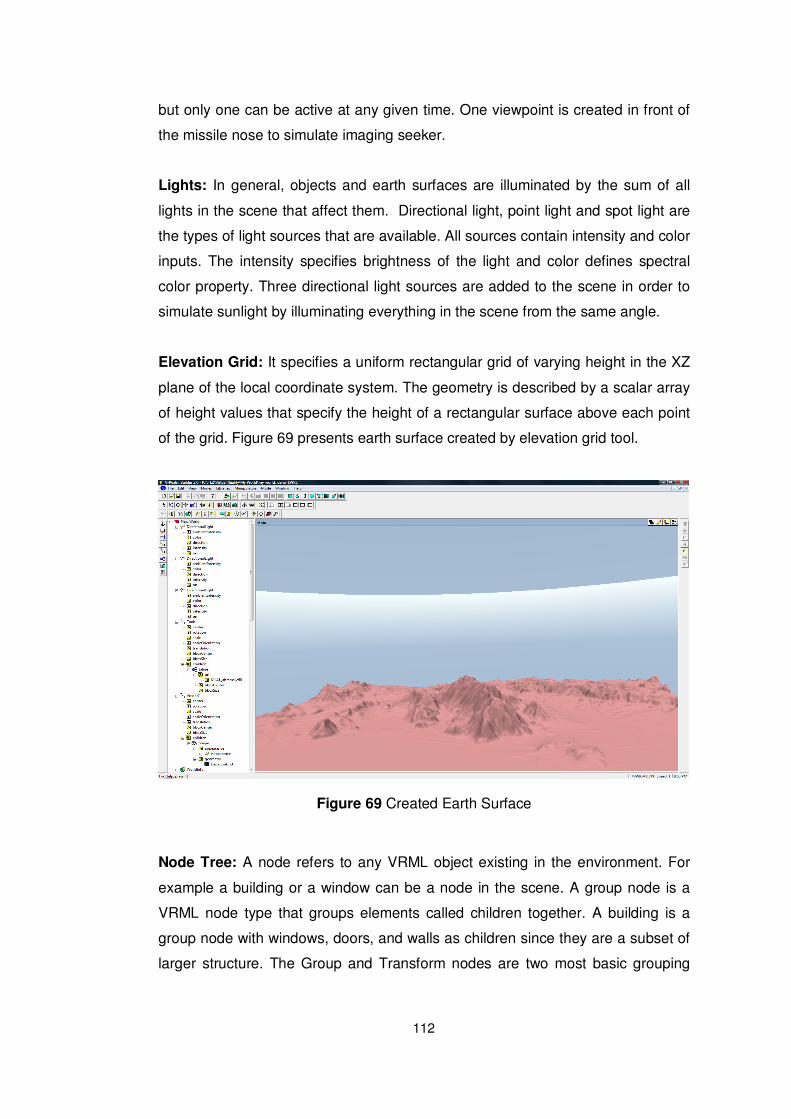
112
but only one can be active at any given time. One viewpoint is created in front of
the missile nose to simulate imaging seeker.
Lights: In general, objects and earth surfaces are illuminated by the sum of all
lights in the scene that affect them. Directional light, point light and spot light are
the types of light sources that are available. All sources contain intensity and color
inputs. The intensity specifies brightness of the light and color defines spectral
color property. Three directional light sources are added to the scene in order to
simulate sunlight by illuminating everything in the scene from the same angle.
Elevation Grid: It specifies a uniform rectangular grid of varying height in the XZ
plane of the local coordinate system. The geometry is described by a scalar array
of height values that specify the height of a rectangular surface above each point
of the grid. Figure 69 presents earth surface created by elevation grid tool.
Figure 69 Created Earth Surface
Node Tree: A node refers to any VRML object existing in the environment. For
example a building or a window can be a node in the scene. A group node is a
VRML node type that groups elements called children together. A building is a
group node with windows, doors, and walls as children since they are a subset of
larger structure. The Group and Transform nodes are two most basic grouping
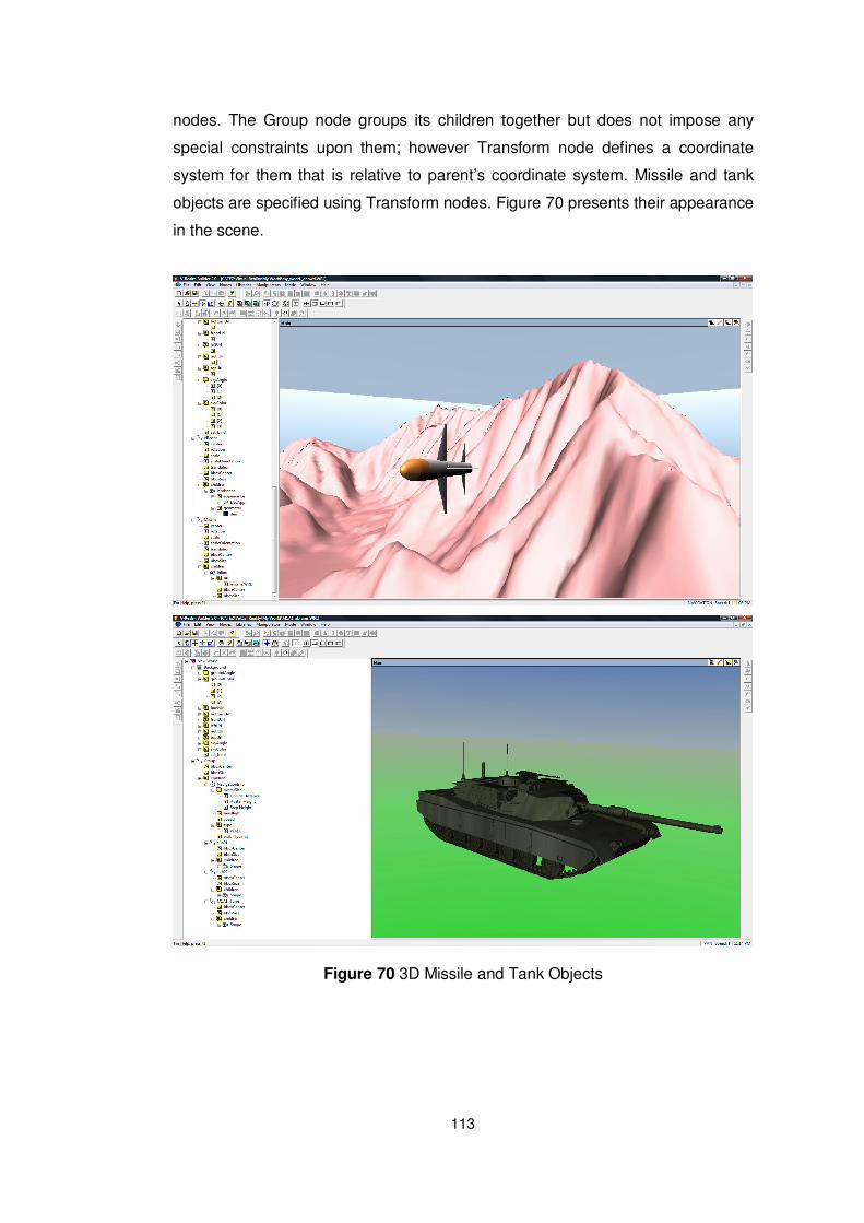
113
nodes. The Group node groups its children together but does not impose any
special constraints upon them; however Transform node defines a coordinate
system for them that is relative to parent’s coordinate system. Missile and tank
objects are specified using Transform nodes. Figure 70 presents their appearance
in the scene.
Figure 70 3D Missile and Tank Objects