Autonomous Mobile Robot Design

Dr. Kostas Alexis (CSE)

Topic: State Estimation

World state (or system state)

Belief state:

Our belief/estimate of the world state

World state:

Real state of the robot in the real world

Parts of this talk are inspired from the edX lecture “Autonomous Navigation for Flying Robots” from TUM

State Estimation

What parts of the world state are (most) relevant for a flying robot?

Position

Velocity

Orientation

Attitude rate

Obstacles

Map

Positions and intentions of other robots/human beings

…

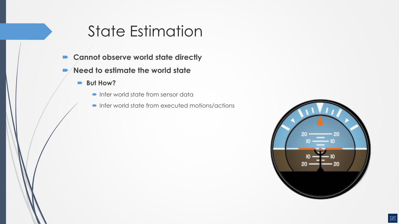
State Estimation

Cannot observe world state directly

Need to estimate the world state

But How?

Infer world state from sensor data

Infer world state from executed motions/actions

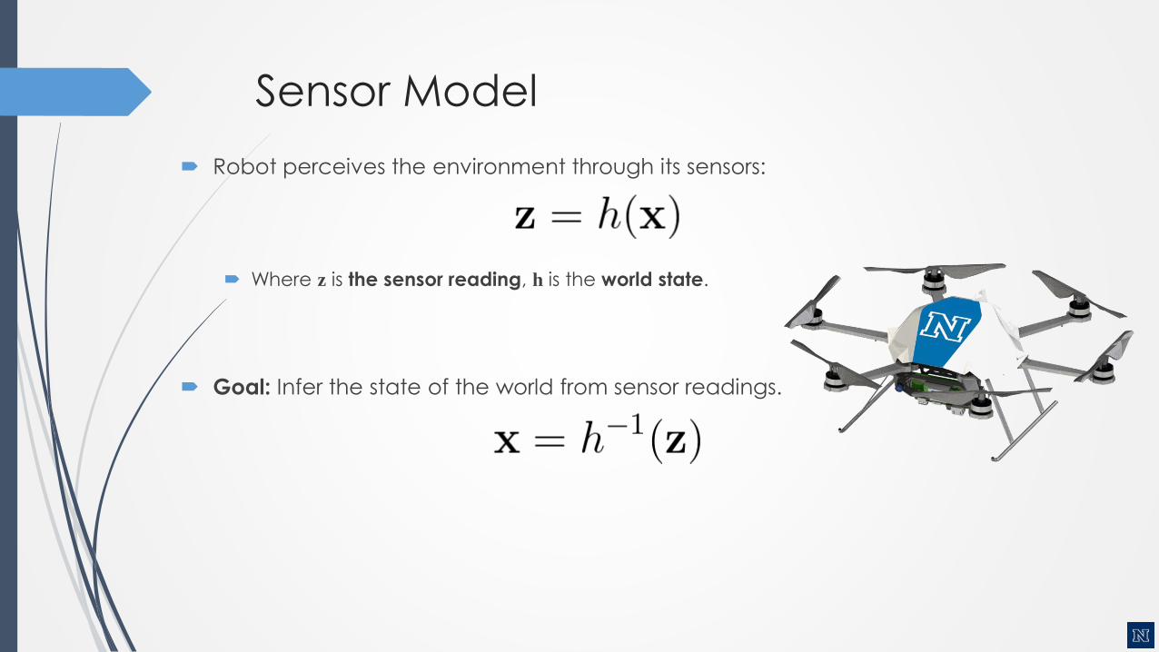
Sensor Model

Robot perceives the environment through its sensors:

Where z is the sensor reading, h is the world state.

Goal: Infer the state of the world from sensor readings.

Motion Model

Robot executes an action (or control) u

e.g: move forward at 1m/s

Update belief state according to the motion model:

Where x’ is the current state and x is the previous state.

Probabilistic Robotics

Sensor observations are noisy, partial, potentially missing.

All models are partially wrong and incomplete.

Usually we have prior knowledge.

Probabilistic Robotics

Probabilistic sensor models:

Probabilistic motion models:

Fuse data between multiple sensors (multi-modal):

Fuse data over time (filtering):

Autonomous Mobile Robot Design

Dr. Kostas Alexis (CSE)

Topic: State Estimation – Recap on Probabilities

Probability theory

Random experiment that can produce a number of outcomes, e.g. a rolling

dice.

Sample space, e.g.: {1,2,3,4,5,6}

Event A is subset of outcomes, e.g. {1,3,5}

Probability P(A), e.g. P(A)=0.5

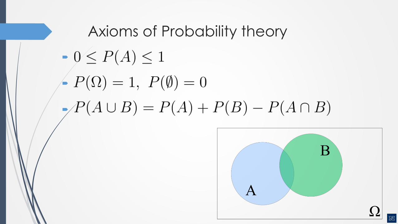
Axioms of Probability theory

Discrete Random Variables

X denotes a random variable

X can take on a countable number of values in {x1,x2,…,xn}

P(X=xi) is the probability that the random variable X takes on value xi

P(.) is called the probability mass function

Example: P(Room)=<0.6,0.3,0.06,0.03>, Room one of the office, corridor, lab,

kitchen

Continuous Random Variables

X takes on continuous values.

P(X=x) or P(x) is called the probability density function (PDF).

Example:

Thrun, Burgard, Fox, “ProbabilisticRobotics”, MIT Press, 2005

Proper Distributions Sum To One

Discrete Case

Continuous Case

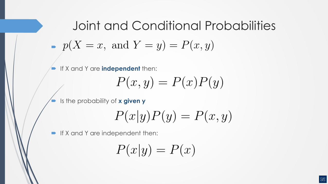
Joint and Conditional Probabilities

If X and Y are independent then:

Is the probability of x given y

If X and Y are independent then:

Conditional Independence

Definition of conditional independence:

Equivalent to:

Note: this does not necessarily mean that:

Marginalization

Discrete case:

Continuous case:

Marginalization example

Expected value of a Random Variable

Discrete case:

Continuous case:

The expected value is the weighted average of all values a random variable

can take on.

Expectation is a linear operator:

Covariance of a Random Variable

Measures the square expected deviation from the mean:

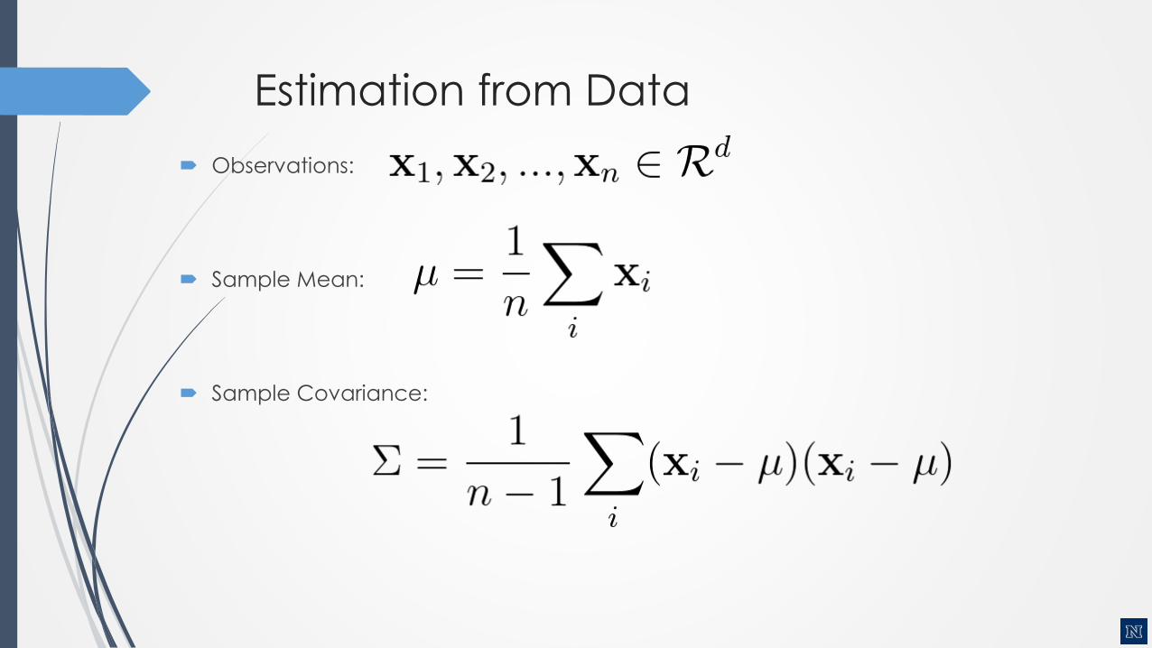
Estimation from Data

Observations:

Sample Mean:

Sample Covariance:

Autonomous Mobile Robot Design

Dr. Kostas Alexis (CSE)

Topic: State Estimation – Reasoning with Bayes Law

The State Estimation problem

We want to estimate the world state x from:

Sensor measurements z and

Controls u

We need to model the relationship between these random variables, i.e:

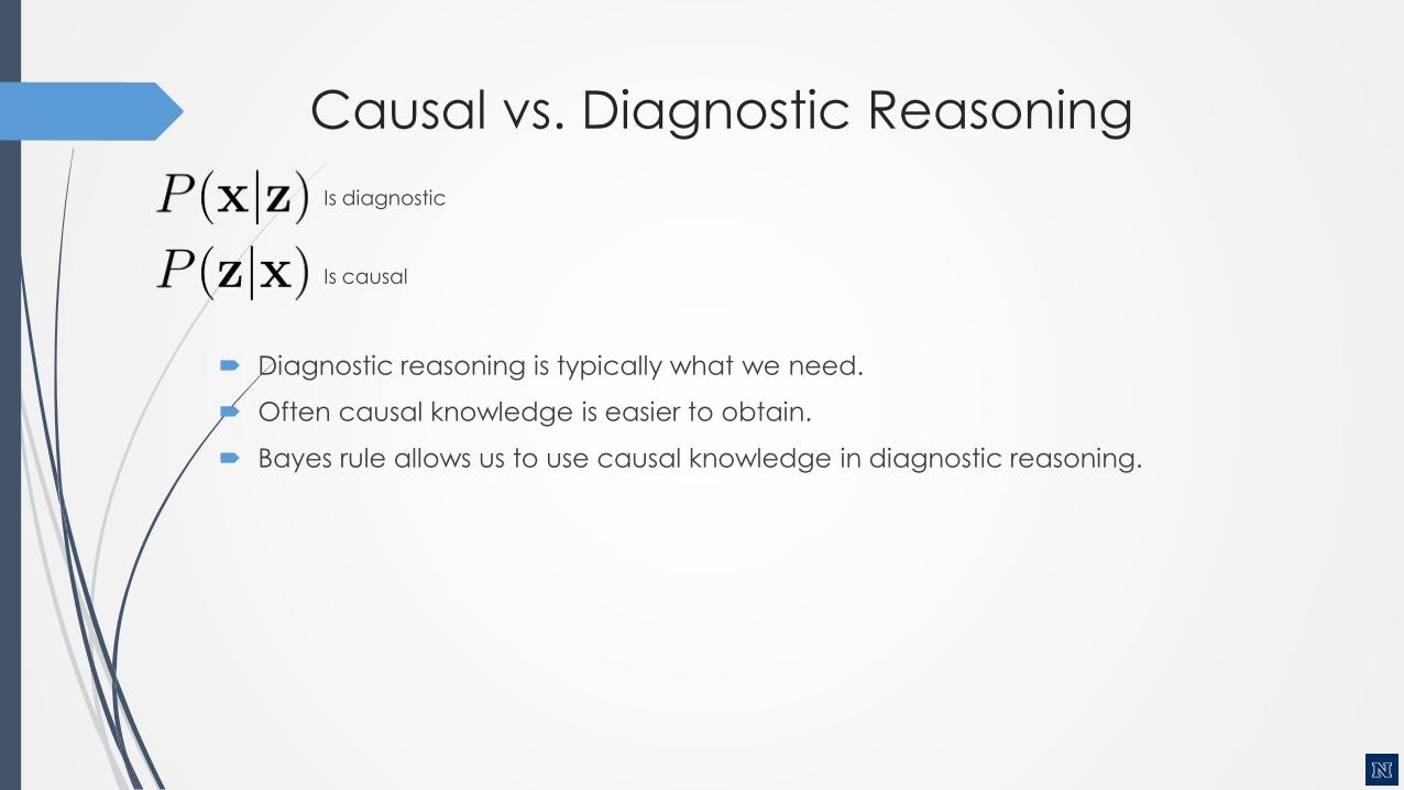
Causal vs. Diagnostic Reasoning

Is diagnostic

Is causal

Diagnostic reasoning is typically what we need.

Often causal knowledge is easier to obtain.

Bayes rule allows us to use causal knowledge in diagnostic reasoning.

Bayes rule

Definition of conditional probability:

Bayes rule:

Observation likelihood Prior on world state

Prior on sensor observations

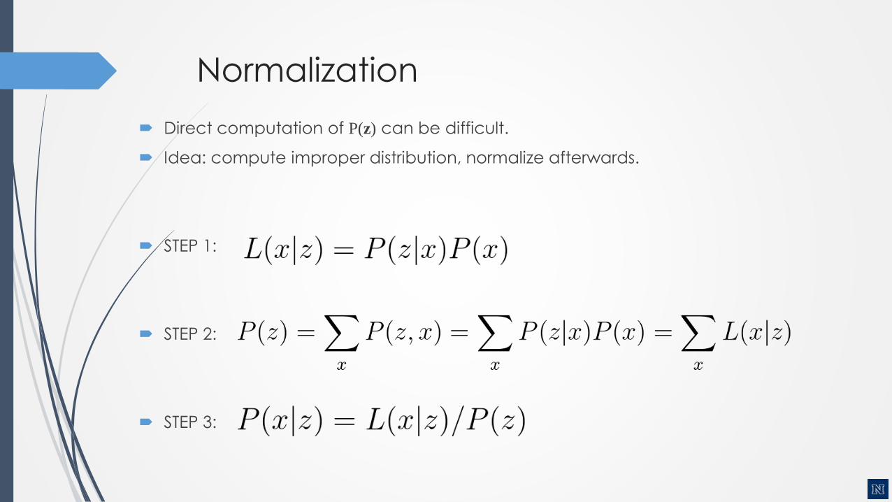
Normalization

Direct computation of P(z) can be difficult.

Idea: compute improper distribution, normalize afterwards.

STEP 1:

STEP 2:

STEP 3:

Normalization

Direct computation of P(z) can be difficult.

Idea: compute improper distribution, normalize afterwards.

STEP 1:

STEP 2:

STEP 3:

Example: Sensor Measurement

Quadrotor seeks the Landing Zone

The landing zone is marked with many bright lamps

The quadrotor has a light sensor.

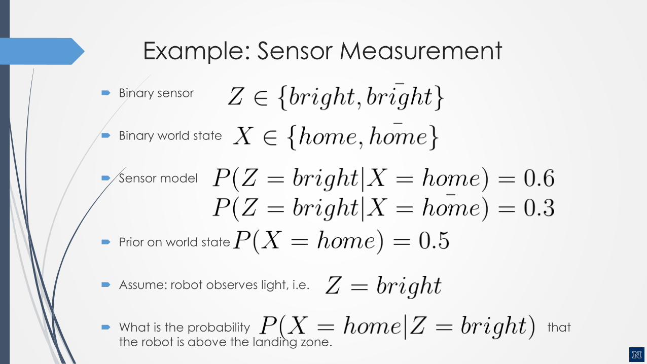
Example: Sensor Measurement

Binary sensor

Binary world state

Sensor model

Prior on world state

Assume: robot observes light, i.e.

What is the probability that

the robot is above the landing zone.

Example: Sensor Measurement

Sensor model:

Prior on world state:

Probability after observation (using Bayes):

Autonomous Mobile Robot Design

Dr. Kostas Alexis (CSE)

Topic: State Estimation – Bayes Filter

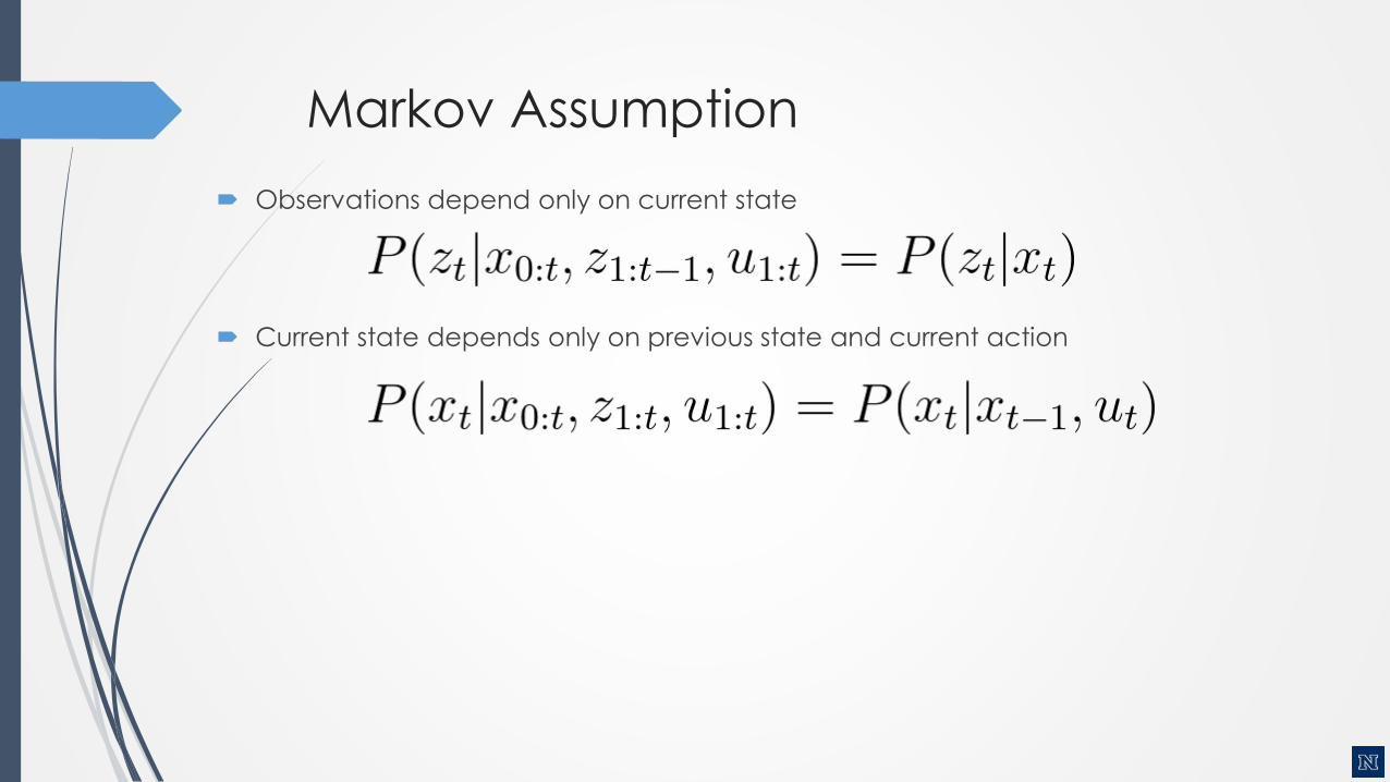
Markov Assumption

Observations depend only on current state

Current state depends only on previous state and current action

Markov Chain

A Markov Chain is a stochastic process where, given the present state, the

past and the future states are independent.

Underlying Assumptions

Static world

Independent noise

Perfect model, no approximation errors

Bayes Filter

Given

Sequence of observations and actions:

Sensor model:

Action model:

Prior probability of the system state:

Desired

Estimate of the state of the dynamic system:

Posterior of the state is also called belief:

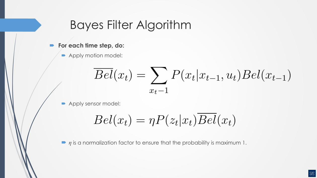
Bayes Filter Algorithm

For each time step, do:

Apply motion model:

Apply sensor model:

η is a normalization factor to ensure that the probability is maximum 1.

Notes

Bayes filters also work on continuous state spaces (replace sum by integral).

Bayes filter also works when actions and observations are asynchronous.

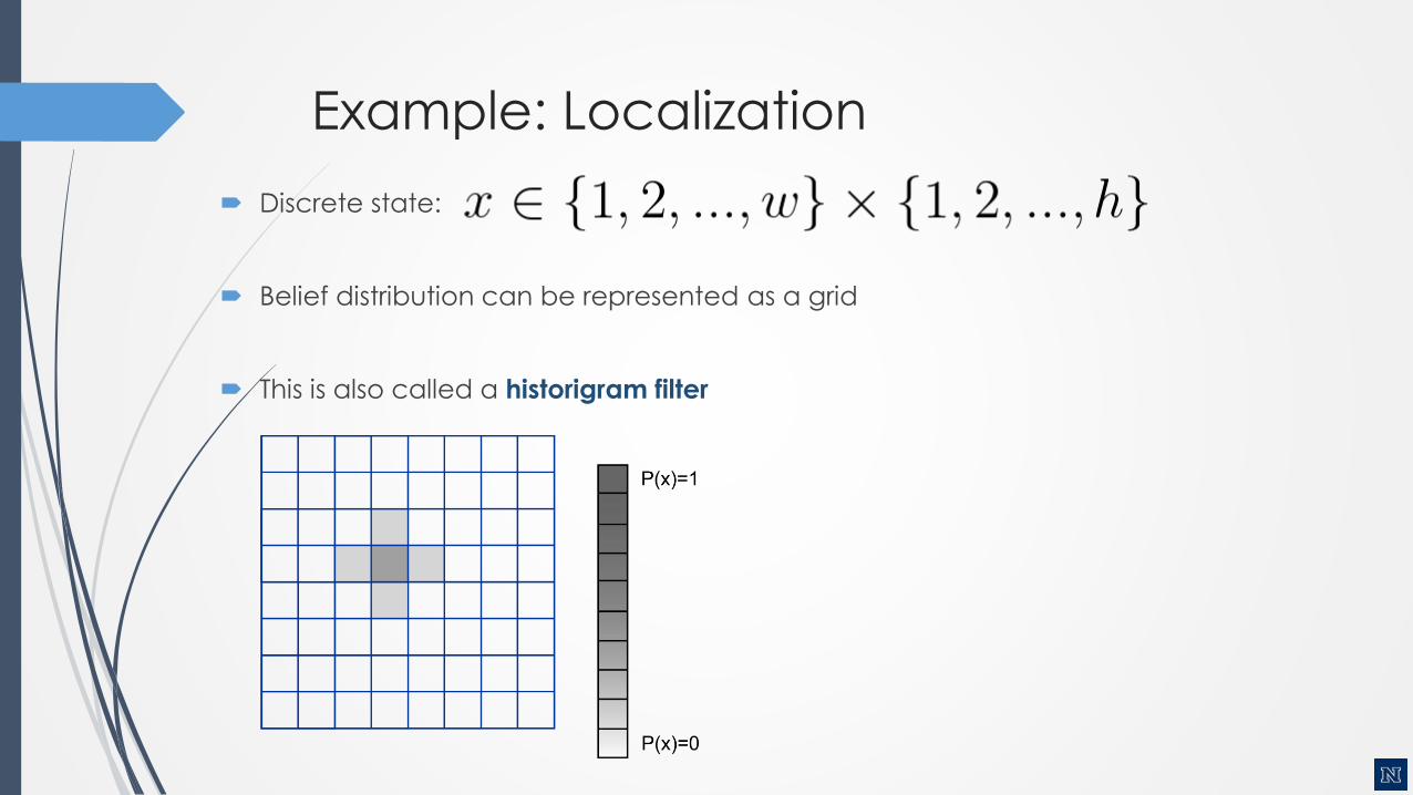
Example: Localization

Discrete state:

Belief distribution can be represented as a grid

This is also called a historigram filter

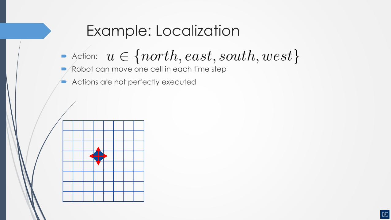
Example: Localization

Action:

Robot can move one cell in each time step

Actions are not perfectly executed

Example: Localization

Action

Robot can move one cell in each time step

Actions are not perfectly executed

Example: move east

60% success rate, 10% to stay/move too far/ move one up/ move one down

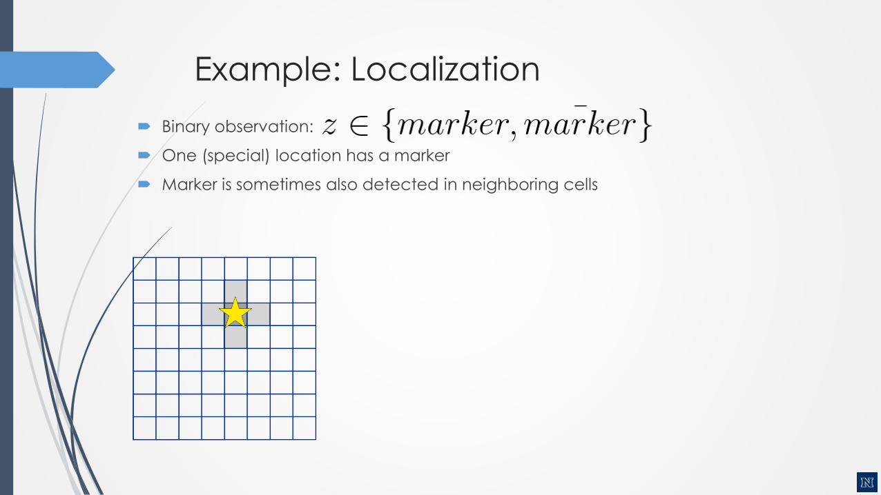
Example: Localization

Binary observation:

One (special) location has a marker

Marker is sometimes also detected in neighboring cells

Example: Localization

Let’s start a simulation run…

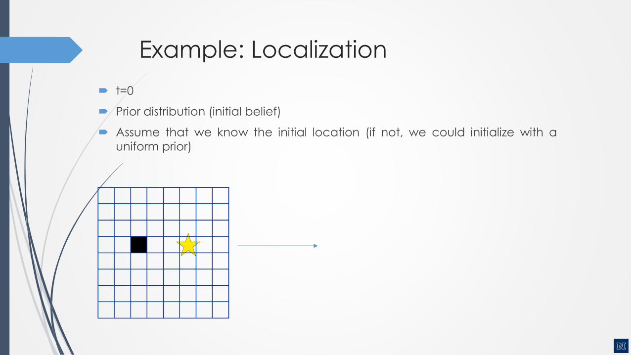
Example: Localization

t=0

Prior distribution (initial belief)

Assume that we know the initial location (if not, we could initialize with a

uniform prior)

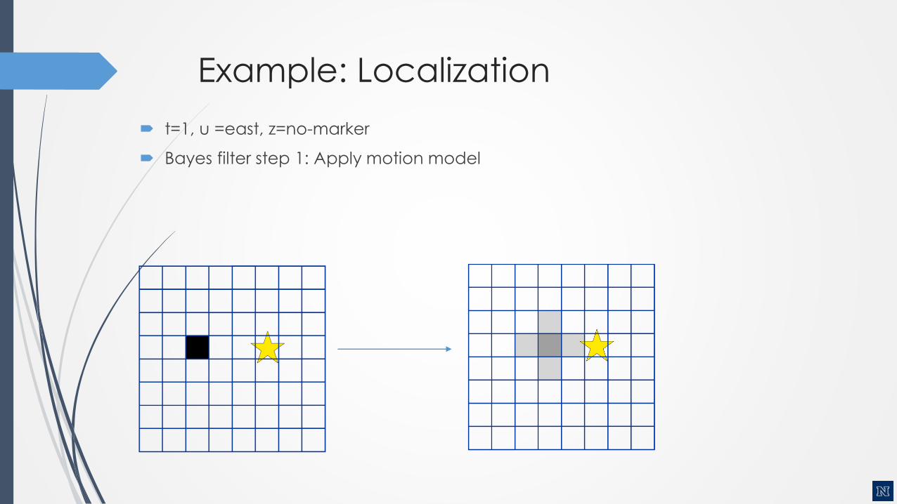
Example: Localization

t=1, u =east, z=no-marker

Bayes filter step 1: Apply motion model

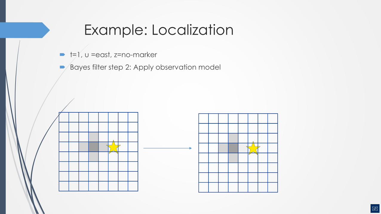
Example: Localization

t=1, u =east, z=no-marker

Bayes filter step 2: Apply observation model

Example: Localization

t=2, u =east, z=marker

Bayes filter step 1: Apply motion model

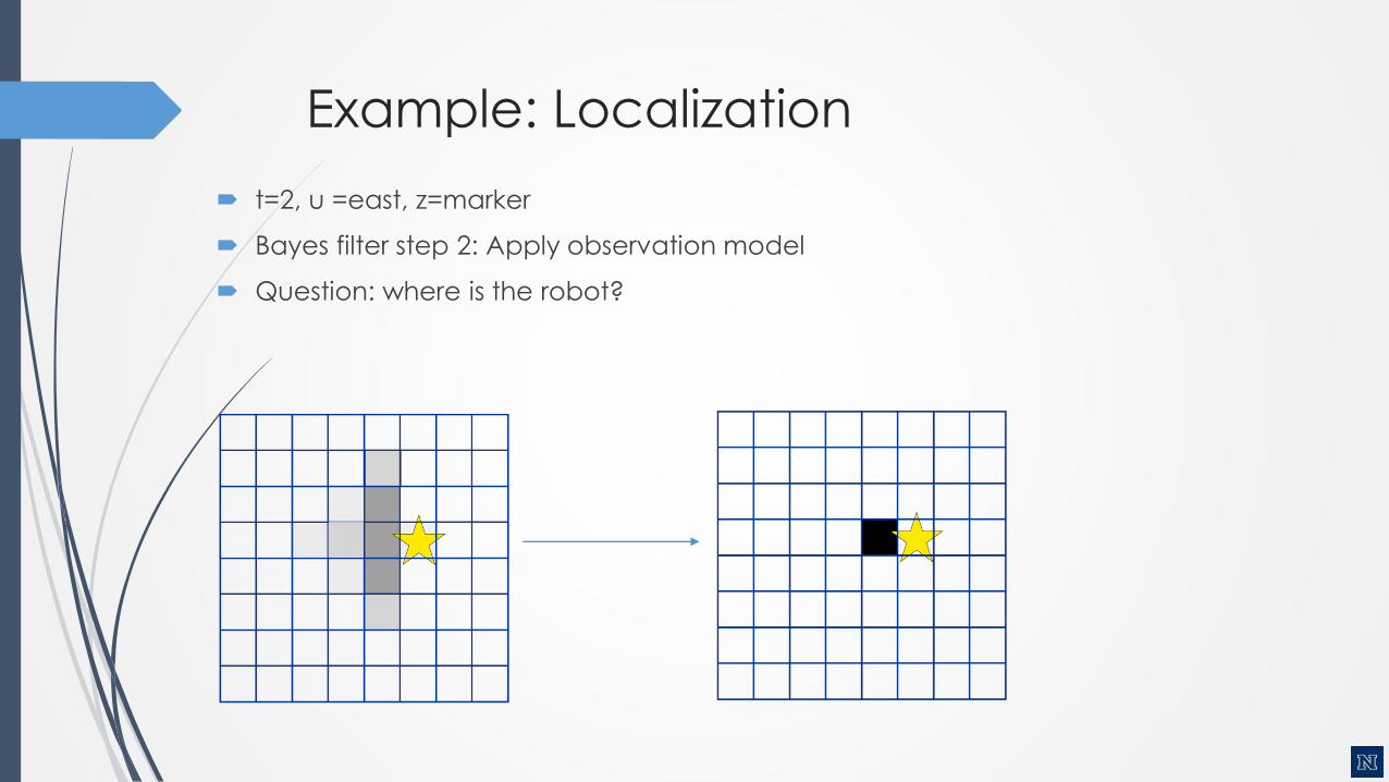
Example: Localization

t=2, u =east, z=marker

Bayes filter step 2: Apply observation model

Question: where is the robot?

Autonomous Mobile Robot Design

Dr. Kostas Alexis (CSE)

Topic: State Estimation – Kalman Filter

Kalman Filter

Bayes filter is a useful tool for state estimation.

Histogram filter with grid representation is not very efficient.

How can we represent the state more efficiently?

Kalman Filter

Bayes filter with continuous states

State represented with a normal distribution

Developed in the late 1950’s. A cornerstone. Designed and first application:

estimate the trajectory of the Apollo missiles.

Kalman Filter is very efficient (only requires a few matrix operations per time

step).

Applications range from economics, weather forecasting, satellite

navigation to robotics and many more.

Kalman Filter

Univariate distribution

mean

Variance (squared

standard deviation)

Kalman Filter

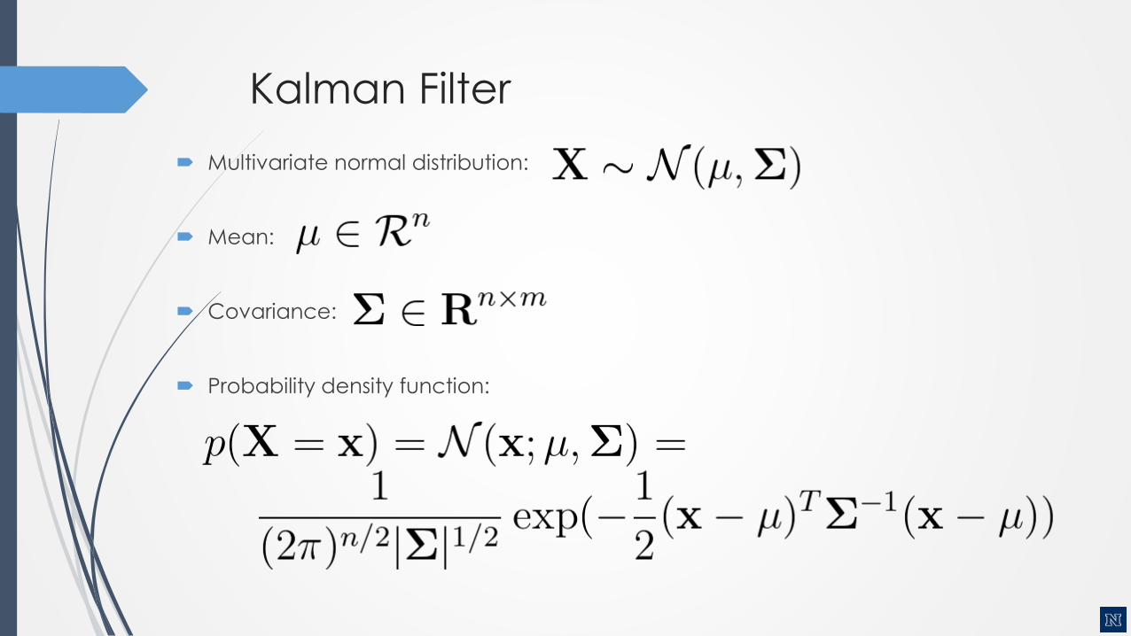
Multivariate normal distribution:

Mean:

Covariance:

Probability density function:

Properties of Normal Distributions

Linear transformation – remains Gaussian

Intersection of two Gaussians – remains Gaussian

Properties of Normal Distributions

Linear transformation – remains Gaussian

Intersection of two Gaussians – remains Gaussian

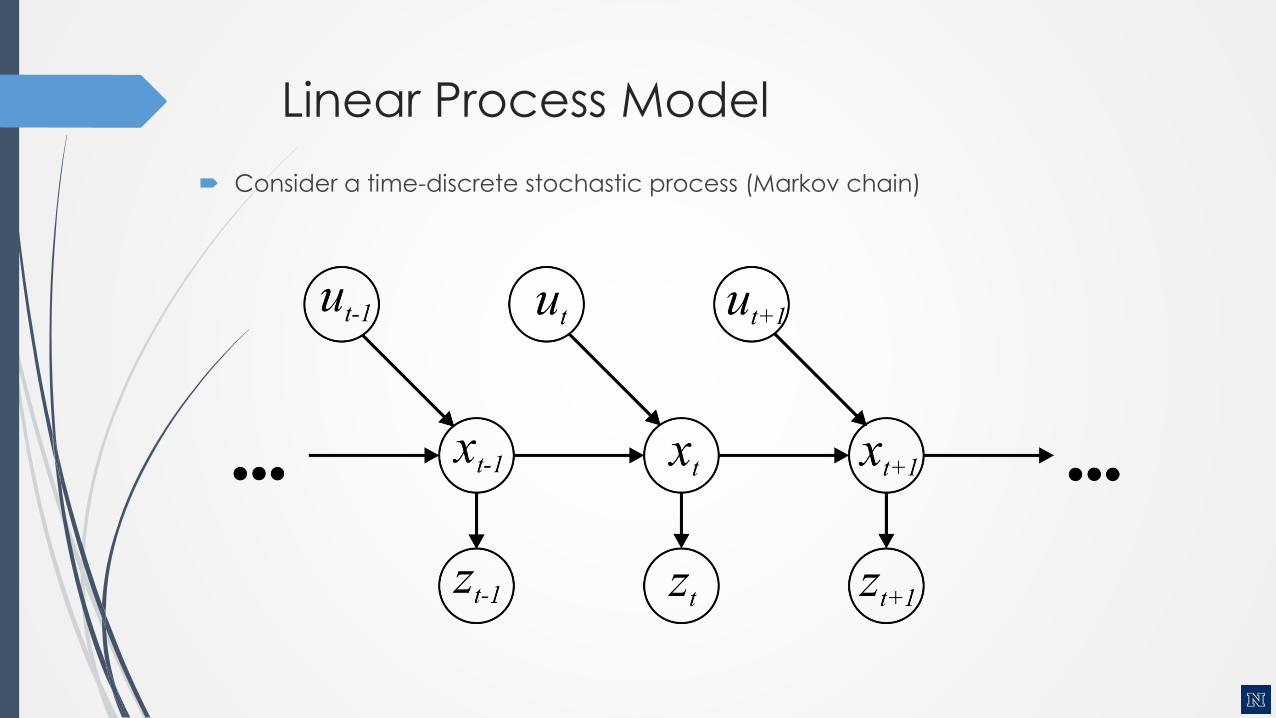
Linear Process Model

Consider a time-discrete stochastic process (Markov chain)

Linear Process Model

Consider a time-discrete stochastic process

Represent the estimated state (belief) with a Gaussian

Linear Process Model

Consider a time-discrete stochastic process

Represent the estimated state (belief) with a Gaussian

Assume that the system evolves linearly over time, then

Linear Process Model

Consider a time-discrete stochastic process

Represent the estimated state (belief) with a Gaussian

Assume that the system evolves linearly over time, then depends linearly on

the controls

Linear Process Model

Consider a time-discrete stochastic process

Represent the estimated state (belief) with a Gaussian

Assume that the system evolves linearly over time, then depends linearly on

the controls, and has zero-mean, normally distributed process noise

With

Linear Observations

Further, assume we make observations that depend linearly on the state

Linear Observations

Further, assume we make observations that depend linearly on the state and

that are perturbed zero-mean, normally distributed observation noise

With

Kalman Filter

Estimates the state xt of a discrete-time controlled process that is governed

by the linear stochastic difference equation

And (linear) measurements of the state

With and

Kalman Filter

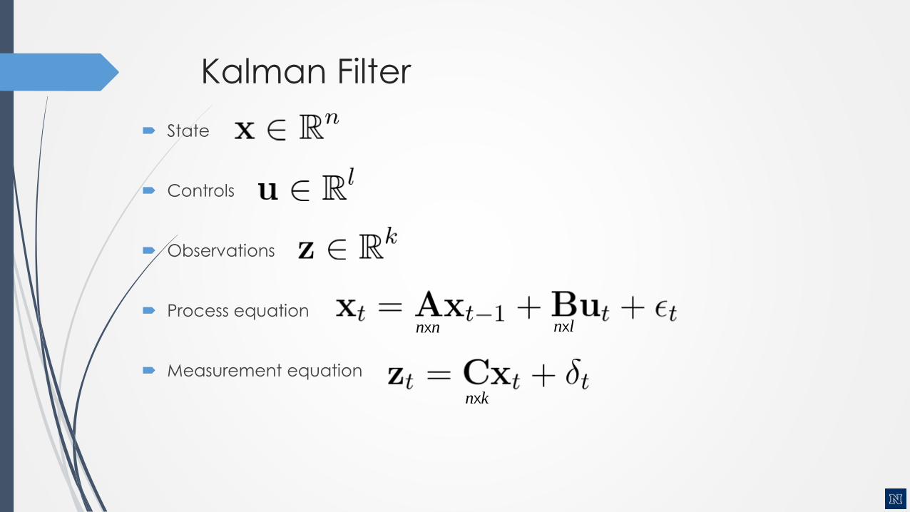
State

Controls

Observations

Process equation

Measurement equation

nxn nxl

nxk

Kalman Filter

Initial belief is Gaussian

Next state is also Gaussian (linear transformation)

Observations are also Gaussian

Recall: Bayes Filter Algorithm

For each step, do:

Apply motion model

Apply sensor model

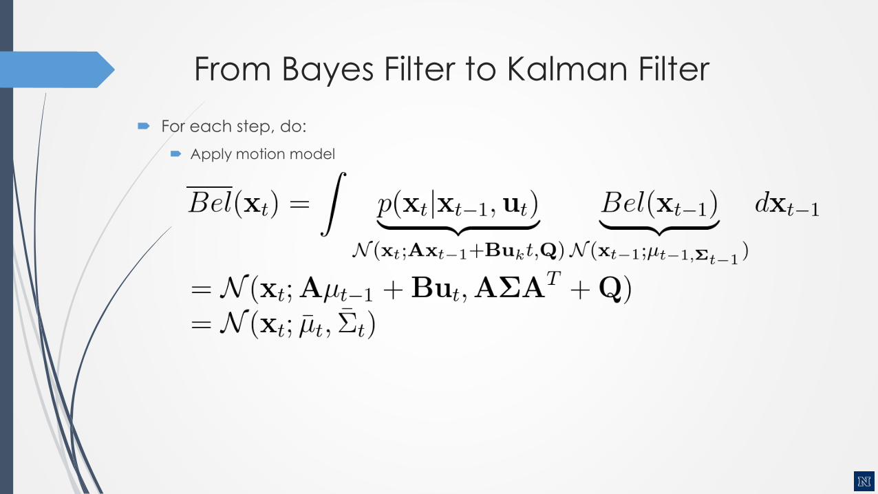
From Bayes Filter to Kalman Filter

For each step, do:

Apply motion model

From Bayes Filter to Kalman Filter

For each step, do:

Apply motion model

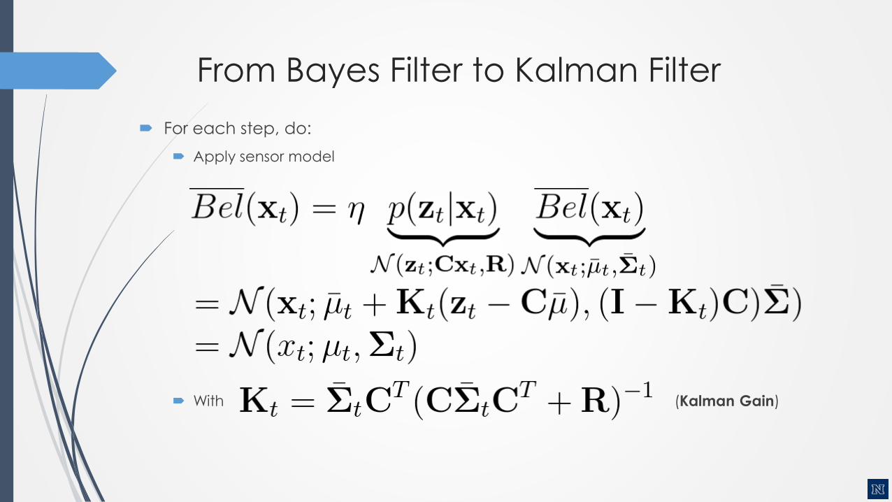
From Bayes Filter to Kalman Filter

For each step, do:

Apply sensor model

With (Kalman Gain)

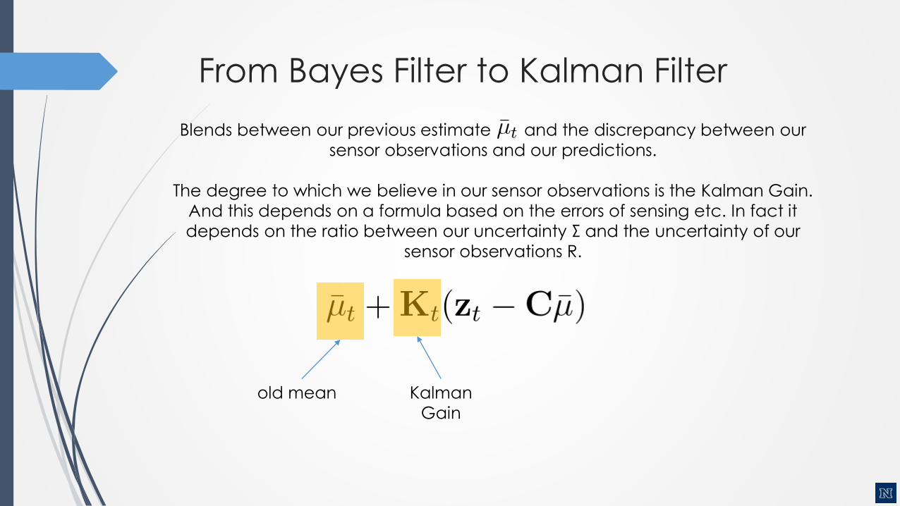
From Bayes Filter to Kalman Filter

old mean Kalman

Gain

Blends between our previous estimate and the discrepancy between our

sensor observations and our predictions.

The degree to which we believe in our sensor observations is the Kalman Gain.

And this depends on a formula based on the errors of sensing etc. In fact it

depends on the ratio between our uncertainty Σ and the uncertainty of our

sensor observations R.

From Bayes Filter to Kalman Filter

For each step, do:

Apply sensor model

With (Kalman Gain)

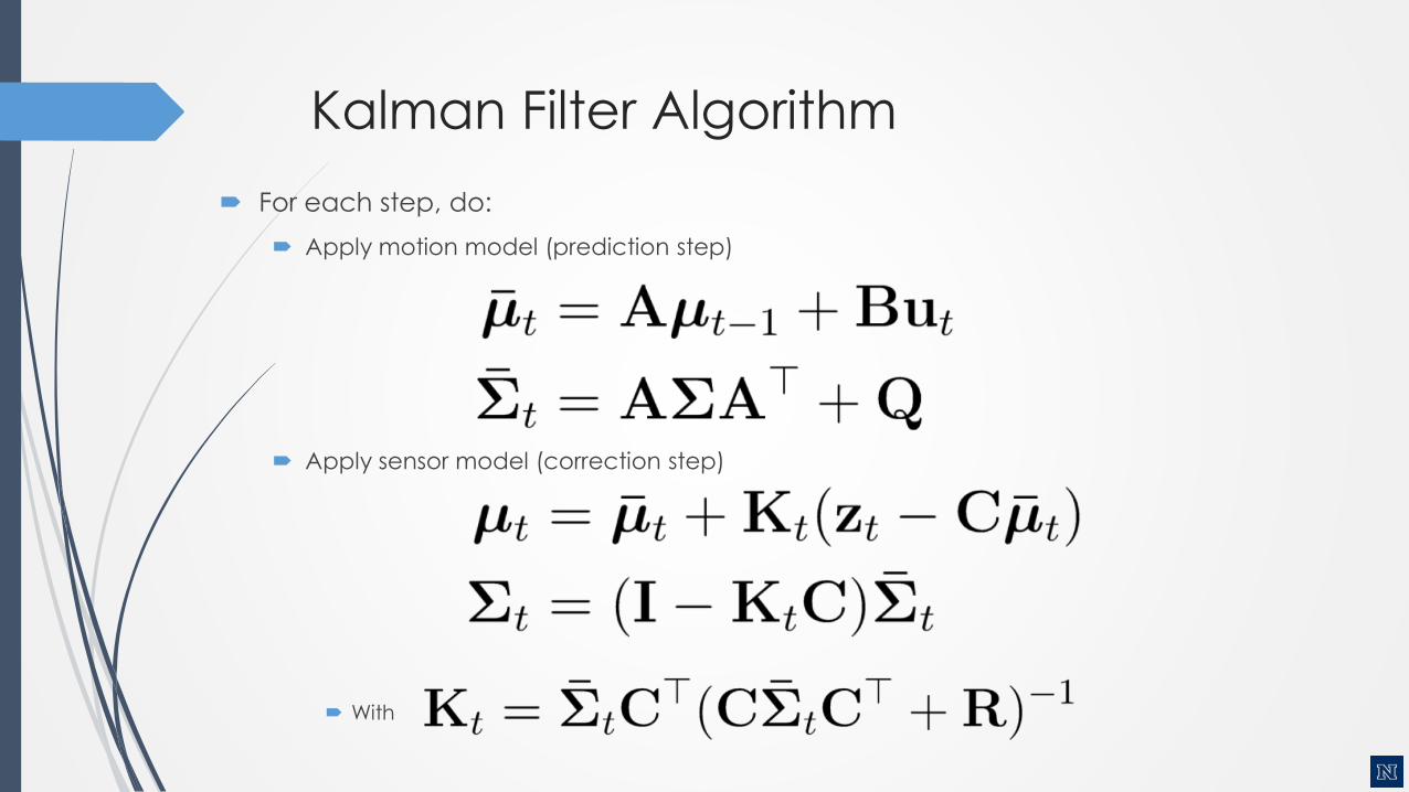
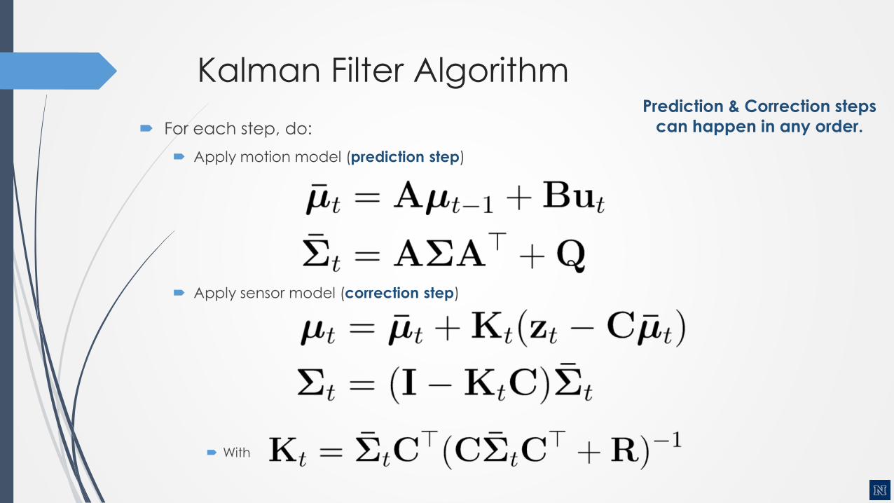
Kalman Filter Algorithm

For each step, do:

Apply motion model (prediction step)

Apply sensor model (correction step)

With

Kalman Filter Algorithm

For each step, do:

Apply motion model (prediction step)

Apply sensor model (correction step)

With

Prediction & Correction steps

can happen in any order.

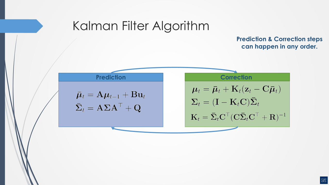
Kalman Filter AlgorithmPrediction & Correction steps

can happen in any order.

Prediction Correction

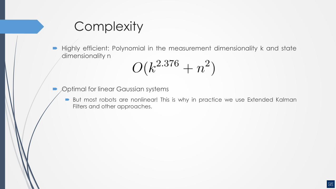
Complexity

Highly efficient: Polynomial in the measurement dimensionality k and state

dimensionality n

Optimal for linear Gaussian systems

But most robots are nonlinear! This is why in practice we use Extended Kalman

Filters and other approaches.

Python KF Implementation

http://www.kostasalexis.com/the-kalman-filter.html

Assignment 1: Estimating a Random Constant

The goal of this task is to estimate a scalar random constant, which may be a voltage level.Let's assume that we have the ability to take measurements of the constant, but that themeasurements are corrupted by 0.1 Volt RMS white measurement noise (e.g. our analog todigital converter is not very accurate). In this example, the process is governed by the lineardifference equation:

with a measurement z that is:

The state does not change from step to step, this is why A=1. There is no control input,therefore B =0,u=0. Our noisy measurement, directly measures the state - therefore H=1.Notice that the subscript k was dropped in several places because the respectiveparameters remain constant in our simple model.

Programming Language: preferably one Python, MATLAB, C++, or JAVA

Form of the Report: 1. Brief report with the code and the relevant plots indicating the correct estimateof the constant, 2. Comments on what you understood about the filter operation.

Deadline: March 11, 2016

Code Examples and Tasks

KF, EKF, UKF

Kalman Filter: https://github.com/unr-

arl/autonomous_mobile_robot_design_course/tree/master/matlab

/state-estimation/kalman-filter

Extended Kalman Filter: https://github.com/unr-

arl/autonomous_mobile_robot_design_course/tree/master/matlab

/state-estimation/extended-kalman-filter

Unscented Kalman Filter: https://github.com/unr-

arl/autonomous_mobile_robot_design_course/tree/master/matlab

/state-estimation/unscented-kalman-filter

How does this apply to my project?

State estimation is the way to use robot sensors to infer the robot state. You

will use it for estimating your robot pose or its map, to track and object and

be able to follow it etc.

Find out more

http://www.kostasalexis.com/the-kalman-filter.html

http://aerostudents.com/files/probabilityAndStatistics/probabilityTheoryFullV

ersion.pdf

http://www.cs.unc.edu/~welch/kalman/

http://home.wlu.edu/~levys/kalman_tutorial/

https://github.com/rlabbe/Kalman-and-Bayesian-Filters-in-Python

http://www.kostasalexis.com/literature-and-links.html

Thank you! Please ask your question!