Autonomous Hexacopter Software Design

Michael Baxter 20503664

Supervisors: Prof. Dr. Thomas Braünl

Mr Chris Croft

Final Year Project Report School of Electrical, Electronic and Computer Engineering

University of Western Australia

28th October 2014

1

Contents Abstract .......................................................................................................................... 3

Acknowledgements ........................................................................................................ 4

1. Introduction and background .................................................................................. 5

1.1 Introduction ..................................................................................................... 5 1.2 Motivation ....................................................................................................... 5 1.3 Background ..................................................................................................... 6 1.4 Goals / design problem .................................................................................... 7

2. Literature review ..................................................................................................... 8

2.1 Sensors and hardware ...................................................................................... 8 2.2 Modeling ......................................................................................................... 9 2.3 Pose estimation and sensor fusion ................................................................. 10 2.4 Control loops ................................................................................................. 10 2.5 Goal setting ................................................................................................... 10

3. System Overview .................................................................................................. 11

3.1 Hardware system ........................................................................................... 11 3.2 Software system ............................................................................................ 12 3.3 Communication system ................................................................................. 14

4. GPS based navigation ........................................................................................... 16

4.1 Distance and bearing calculations ................................................................. 16 4.2 Direct flight vector method ........................................................................... 17 4.3 Waypoint following algorithm ...................................................................... 18

5. Camera based navigation ...................................................................................... 19

5.1 HSV thresholding .......................................................................................... 19 5.2 Single coloured object detection ................................................................... 20 5.3 Coloured object tracking ............................................................................... 20

6. Results and discussion .......................................................................................... 22

6.1 GPS-based navigation ................................................................................... 22 6.2 Camera based navigation .............................................................................. 23 6.3 Discussion of practical issues and problems encountered when using the raspberry pi on a hexacopter platform ..................................................................... 26

2

7. Alternative flight vector methods ......................................................................... 28

7.1 Intermediate goal flight vectoring ................................................................. 28 7.2 Improved direct flight vectoring ................................................................... 29 7.3 Line following flight vectoring ..................................................................... 30 7.4 Curve following............................................................................................. 32

8. Conclusions and future work ................................................................................ 36

8.1 Conclusions ................................................................................................... 36 8.2 Future work ................................................................................................... 36

9. Reference list ........................................................................................................ 37

3

Abstract Multirotor unmanned aerial vehicles are a popular up and coming platform for

autonomous robotics research. This report outlines the design and implementation of

a multithreaded software system for a hexacopter controlled by a raspberry pi.

An array of sensors including a GPS, an IMU and a camera are used on the

hexacopter, and the software system is responsible for collecting data from and

monitoring these sensors through their lower level libraries. A modular approach is

taken to software design so that the system can be used in a variety of applications.

The applications tested in this project were: GPS waypoint navigation and single

coloured object tracking. GPS navigation was achieved with a maximum path

deviation of 5.66m. A discussion on improvements to the navigation algorithm and

the incorporation of course correction methods is provided. Object tracking

algorithms were implemented using center of mass and camshift techniques, which

were optimized using HSV thresholding, lookup tables and reduced colour spaces.

The hexacopter was able to track a red object moving at a slow waking pace for a full

trial, 1.13 minutes in length.

The software system presented is flexible, currently in use with other simultaneous

projects and sets out a framework for future development.

4

Acknowledgements

I would like to thank the following people for their contributions to this project:

My supervisors Mr Chris Croft and Prof. Thomas Braünl for their advice and

guidance with this project.

Chris  Venables  and  Rory  O’Connor  for  the  work  on  the  project  in  2013  and  getting  it  

off the ground, literally.

Tom Drage for his help and support.

Fellow group members: Omid Targhagh, Alex Mazur and Merrick Cloete for their

contributions to the project.

Gordon Henderson, Richard G. Hirst, Emil Valkov, the OpenCV team, the Boost

team, Ariandy, Migiel Grindberg and the mjpg-streamer team for the software

libraries used throughout the project.

5

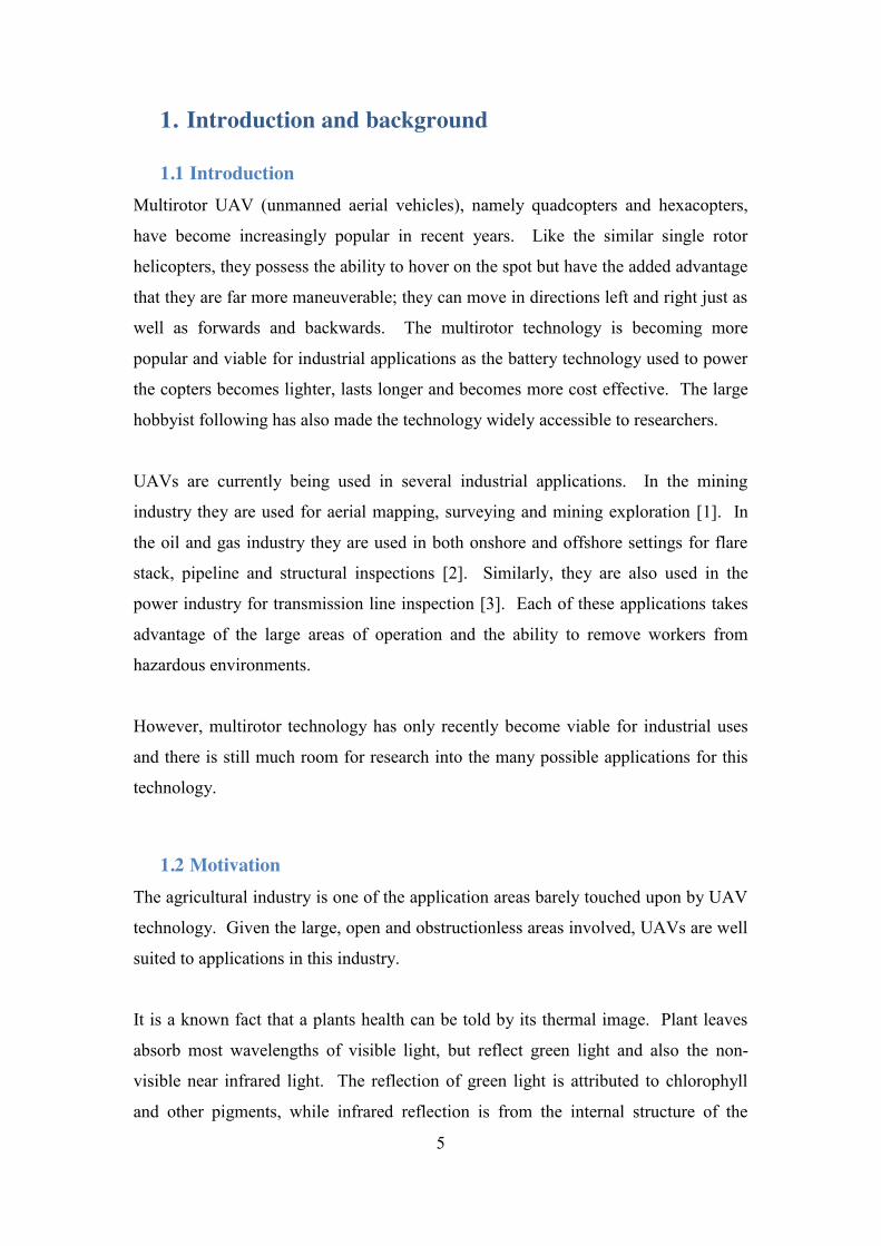
1. Introduction and background

1.1 Introduction Multirotor UAV (unmanned aerial vehicles), namely quadcopters and hexacopters,

have become increasingly popular in recent years. Like the similar single rotor

helicopters, they possess the ability to hover on the spot but have the added advantage

that they are far more maneuverable; they can move in directions left and right just as

well as forwards and backwards. The multirotor technology is becoming more

popular and viable for industrial applications as the battery technology used to power

the copters becomes lighter, lasts longer and becomes more cost effective. The large

hobbyist following has also made the technology widely accessible to researchers.

UAVs are currently being used in several industrial applications. In the mining

industry they are used for aerial mapping, surveying and mining exploration [1]. In

the oil and gas industry they are used in both onshore and offshore settings for flare

stack, pipeline and structural inspections [2]. Similarly, they are also used in the

power industry for transmission line inspection [3]. Each of these applications takes

advantage of the large areas of operation and the ability to remove workers from

hazardous environments.

However, multirotor technology has only recently become viable for industrial uses

and there is still much room for research into the many possible applications for this

technology.

1.2 Motivation The agricultural industry is one of the application areas barely touched upon by UAV

technology. Given the large, open and obstructionless areas involved, UAVs are well

suited to applications in this industry.

It is a known fact that a plants health can be told by its thermal image. Plant leaves

absorb most wavelengths of visible light, but reflect green light and also the non-

visible near infrared light. The reflection of green light is attributed to chlorophyll

and other pigments, while infrared reflection is from the internal structure of the

6

plants leaves [4]. Unhealthy plants reflect less infrared light and this difference can

be detected remotely using a thermal imaging camera.

Causes for unhealthy plants include: disease, pest infestation, frost and water stress

[5]. This leads to practical applications, for example: pesticides can be selectively

applied only to affected regions and irrigation blockages can be detected remotely and

fixed early.

UAVs are being used in conjunction with thermal cameras in an agricultural setting

[6], but the process is yet to be autotomized. The motivation for this project is to

combine the two technologies of autonomous flight and intelligent image processing

to produce a machine that will identify areas of interest in real time and carry out

autonomously inspection.

1.3 Background This project is building onto the efforts of Venables [7] and  O’Connor [8], who in

2013 constructed the hexacopter from a hobbyist kit and demonstrated its capabilities

in autonomous flight with onboard navigation and image processing algorithms.

This  year’s  project  was  adopted  by  myself  and  3  other  students.    The  project  is  split  

into 4 components:

x Myself – Core software system involving interactions with sensors and

actuators.

x Omid Targhagh – GPS based navigation including trajectory planning and

intelligent search patterns.

x Merrick Cloete – Onboard image processing and object detection.

x Alex Mazur – Web based user interface and integration of all parts.

7

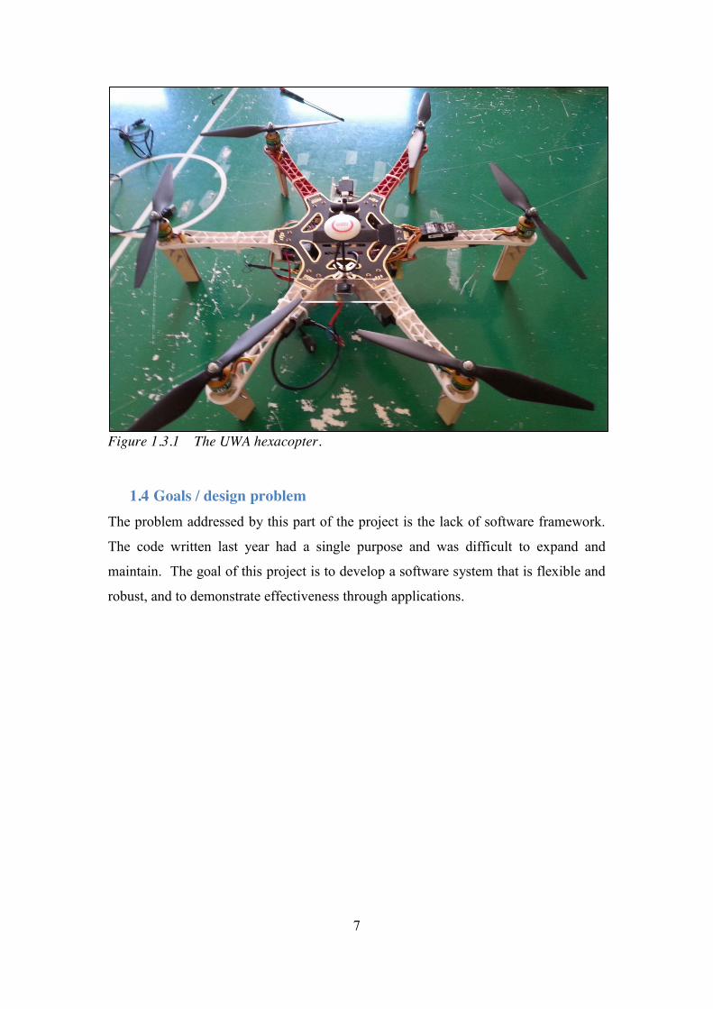
Figure 1.3.1 The UWA hexacopter.

1.4 Goals / design problem The problem addressed by this part of the project is the lack of software framework.

The code written last year had a single purpose and was difficult to expand and

maintain. The goal of this project is to develop a software system that is flexible and

robust, and to demonstrate effectiveness through applications.

8

2. Literature review Multirotor UAVs are a keen platform for many autonomous aerial robotics research

projects. Of the literature surveyed, research divides into either indoor applications,

mainly employing a vision based navigation system, or outdoor applications using

GPS based navigation. Common across the literature are the 5 parts of an

autonomous aerial robotic system:

1) Sensors and hardware

2) System modeling

3) Pose estimation and sensor fusion

4) Control loops

5) Goal setting

2.1 Sensors and hardware Nearly all of the projects surveyed used an IMU (inertial measurement unit) [9-17], a

device that contains accelerometers, gyroscopes, magnetometers and an embedded

controller to combine readings   to  provide   information  on   the  UAV’s   roll,  pitch  and  

yaw, as well as accelerations in each direction. The acceleration data can be

integrated to provide positional data, but as discussed in many papers [10, 15, 17], the

accumulation of errors makes readings unreliable without supplementation with other

sensors.

GPS (global positioning system) is most preferred for outdoor applications [13, 15,

17] and provides a positional fix. GPSs suffer from GPS drift, whereby the accuracy

of positional data is restricted to a window and this window shifts due to the number

of GPS satellite signals received and the relative positions of the satellites [15]. This

problem is solved either by combing data with that from an IMU [10, 15, 17] or by

using a differential GPS system [10, 13]. In the differential GPS system, two GPSs

are used, one fixed and the other roving. The GPS drift that effects both can be

canceled out, provided they are kept close enough together and share access to the

same satellite signals.

9

Vision based navigation systems usually employ either a single camera [9] or stereo

cameras [10-12]. In both cases, a technique called optical flow is used for visual

odometry. It involves identifying features in a frame and tracking how much their

positions change throughout successive frames. With knowledge of how far away the

features are and the frame rate, the copters speed is estimated [10, 11]. Stereo vision

lends itself to calculating the distance of the features from the cameras using

perception [10], while other distance sensors such as ultrasound are needed for single

camera systems [9].

A few systems use more advanced mapping systems such as laser scanners [12] and

infrared motion sensors [16]. These are used in SLAM (simultaneous localization and

mapping) systems, whereby the copter navigates relative to its surroundings, mapped

out by scanners.

2.2 Modeling Most copter project have involves kinematic modeling the copter system. The extent

of modeling varies across the literature. The most basic models are based on the

equations of Newtonian motion [9, 15-17]. For a hovering copter, the force of

upward thrust is equal to its weight. The copter moves by adjusting roll and pitch,

such that a component of thrust is in the horizontal plane. Other projects use much

more advanced models, incorporating fluid dynamics [17], blade flap effects [13] and

gyroscopic effects [18].

A novel approach to modeling was taken by [14], in which the tuning process was

automated. The copter was set up in an environment with VICOM infrared tracking

cameras, so that  the  copter’s  pose  was  digitally  known  at  all  times.    Starting  from  the  

first principles model, the copter was instructed to do a flip. The controlling

computer then readjusted the model parameters to match the observed path and the

process reiterated until an accurate model was determined.

10

2.3 Pose estimation and sensor fusion A problem identified across the literature was that sensors are never completely

accurate; the system must estimate its position and orientation (pose) using the best

combination of data available to it. This is solved using a sensor fusion algorithm,

often a variation on the Kalman filter.

The Kalman filter is a two step algorithm. First the next kinematic state of the system

is predicted using a model (as described above) and the previous system state.

Secondly, the state is corrected based on data from the sensors, taking the expected

error of each sensor into account and weighting appropriately using a least squares

regression method. The process repeats so that the estimated state is constantly

refreshed and corrected [19].

The most popular sensor fusion algorithm used across the literature surveyed is

actually the EFK (Extended Kalman Filter) [9-13, 15-17]. The EKF reflects the fact

that most systems are non-linear and cannot be described by the linear model required

by the regular Kalman filter. The EFK uses a non-linear model, but takes the first

order Taylor expansion to make it fit into the Kalman filter framework [19].

2.4 Control loops Traditional PID controllers have been used for both copter stability [13, 14] and for

velocity regulation [9, 13, 14]. Modern control techniques including state variable

feedback [16, 20] and linear quadratic regulator systems [18] have also be used and

found satisfactory.

2.5 Goal setting Higher level goal setting algorithms have been implemented as finite state machines

[9, 12]. The high-level control loop cycles through states representing goals.

Alternately, [16] uses a path manager and represents paths as edges on a graph, which

is incorporated into its SLAM program.

11

3. System Overview

3.1 Hardware system The hexacopter hardware is mostly unchanged since work done in 2013 [7, 8], except

for the upgrade from a raspberry pi model B to a model B+. A brief overview is a

follows: a commercial hexacopter, the DJI flamewheel [21], was purchased, built

from a kit and serves as an experimental platform. This kit includes a flight board

that contains accelerometers and stabilization algorithms. Under normal operation,

RF   (radio   frequency)   signals   are   sent   from   the   handset’s   transmitter   to the RF

receiver, converted to PWM signals and sent to the flight board.

Apart from stabilization, all other autonomous control algorithms are run on the

raspberry pi. The raspberry pi is programmed to output PWM signals mimicking

those produced by the RF receiver. A relay switch was installed to switch between

the two PWM signals, and is controlled by one of the channels of the RF receiver.

The throttle channel (altitude) is not passed through the switch and the operator is in

control  of  the  aircraft’s  altitude at all times. This was done as a safety precaution.

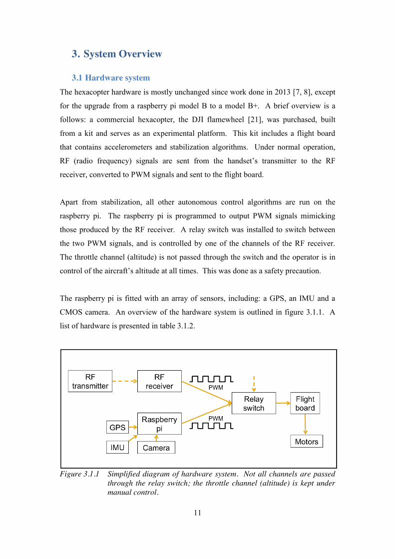
The raspberry pi is fitted with an array of sensors, including: a GPS, an IMU and a

CMOS camera. An overview of the hardware system is outlined in figure 3.1.1. A

list of hardware is presented in table 3.1.2.

Figure 3.1.1 Simplified diagram of hardware system. Not all channels are passed

through the relay switch; the throttle channel (altitude) is kept under manual control.

12

Hardware Brand / model Communication protocol

Library

Flight board DJI / NAZA-M [22] PWM ServoBlaster [23]

GPS Qstarz / BT-Q818X [24] NMEA-0183 wiringPi [25] IMU Xsens / MTi [26] Proprietary serial over

usb Xsens CMT3 [26]

Camera Raspberry pi / Camera module [27]

Serial over 15pin ribbon cable

raspicamCV [28]

Table 3.1.2 List of hardware on hexaopter with communication protocols and software libraries.

A new PIKSI brand differential GPS [29] was trialed for the system. The

manufacturers claim centimeter positional accuracy, however the product is still in its

infancy and the firmware contains too many bugs to be used effectively.

A recent addition to the hexacopter is a low voltage piezo buzzer. This presents the

option of audio feedback for when the copter achieves a goal set out by the top-level

control algorithm.

Communication hardware includes: an analogue video transmitter, a wifi dongle and a

4G dongle. These are discussed in section 3.3.

3.2 Software system In contrast to previous work on this project, a multithreaded approach was taken to

designing the software system. Each sensor has its own background thread that

constantly reads and updates incoming data, whilst monitoring for errors and logging.

This  approach  was  much  inspired  by  Drage’s work on autonomous cars [30]. There is

an emphasis on separating the mid-level system (incorporating data collection and

monitoring of sensors) from the top-level or application level controller, which is

responsible for navigation algorithms and user interactions.

The advantage of this design is that top-level threads can block while waiting for user

input without halting the data gathering threads. Also, this approach is necessary for

integration with the web-based user interface (designed by Mazur), since GPS and

13

orientation data needs to be accessible to both the control systems and for display on

the user interface.

Communication with the flight board was achieved by outputting PWM on the GPIO

pins using the ServoBlaster library written by Hirst [23]. The flight board does not

provide feedback to the raspberry pi. Instead, a copy of the values sent to each

channel is kept and it is assumed that they have been passed to the flight board

correctly. The user does not manipulate the pulse widths of the signals directly; rather

a value is specified between -100 to 100 representing the % power to the channel. For

example 100 on the elevator channel is full power forwards. The values are then

scaled to the appropriate pulse widths.

The GPS is monitored by reading and parsing the character stream read in using the

wiringPi library written by Henderson [25]. The GPS stream is of NMEA [31] format

and an example is provided below. The second, third and fifth values (separated by

commas) are time, latitude and longitude respectively. Other information is also

offered in the NMEA string including the number of satellite signals received and

horizontal dilution; see [31] for more details.

$GPGGA,044130.400,3158.7227,S,11548.9609,E,1,5,11.99,23.8,M,-29.4,M,,*69

The GPS has its own thread that constantly runs it the background, parsing NMEA

messages for appropriate information. The thread also monitors the GPS, and enters

an  error  state  when  the  GPS  is  disconnected,  doesn’t  receive  any  data  after  a  timeout  

period or losses satellite fix. This thread runs at approximately 5Hz, to match the data

rate of the GPS.

The Xsens IMU communicates over RS242 serial over USB through proprietary

CMT3 serial libraries [26]. There were issues with the default data rate being too

high; running the thread at the matched rate caused the thread to hog the CPU

resources, while slowing it down caused data to build up in a buffer (implemented by

the CMT3 library), causing data to be old. Changing the mode of the IMU to

decrease the data transmission rate and running the thread at a matched rate solved

this problem.

14

The IMU was calibrated using the MagfieldMapper program provided by Xsens [26].

The process involved rotating the IMU, whilst in place on the copter, around in as

many different orientations as possible. MagfieldMapper calibrated the IMU

internally against the acceleration due to gravity and the magnetic environment.

Additionally, all image processing is conducted in a self-contained background thread

(the camera is treated as a sensor for coloured objects). Image processing is done

using the OpenCV software libraries [32] and  Valkov’s   RaspiCamCV library [28].

The design criterion for the camera thread is to have the best possible frame rate for a

decent resolution. The focus of the algorithms discussed in section 5 is on efficiency.

Effectiveness and more complex image detection algorithms analyzed in the part of

the project undertaken by Cloete.

The buzzer is operated using a signal from one of the GPIO pins. When activated, a

thread is detached and simulates PWM by turning the pin on and off at frequencies of

up to 100Hz. GPIO manipulation is done using the wiringPi library [25]. This was

chosen over ServoBlaster so that the frequency can be altered without affecting the

pins used for flight board communication. Although the piezo buzzer technically

plays sounds at a single pitch, changing the frequency and pulse width can produce a

noticeable variety of chirps at different volume levels.

3.3 Communication system Three methods of in-flight communication with the raspberry pi were used: direct

connection using Bluetooth keyboard and analogue video transmitter, remote

connection using SSH over a wifi network and communication to a web server over

either wifi or 4G.

Direct communication using the Bluetooth keyboard was the primary communication

method used in 2013 [7]. It involves logging into the raspberry pi on the copter the

same as if it were a desktop computer. In place of a monitor, a video transmitter is

used to send the analogue video to a pair of headset goggles. The goggles can be

plugged into a monitor via RWY connection. Commands are given to the copter

15

through the terminal. Camera vision is streamed by running the X window system

and displaying images on the desktop. This method is effective for up to 20m, the

approximate range of the Bluetooth keyboard.

A similar approach is to remotely log in to the raspberry pi using SSH (secure shell

hosting). This does, however, require a wifi network present, which can either be

provided by a wireless router out on the field, or through an ad hoc network created

by the wifi dongle. Commands are sent through the remote terminal. Camera feed

can be streamed across SSH, but this is slow and laggy (~2fps with a lag of ~3s).

This method can be used for distances up to 30m away, depending on the wifi dongle.

The final communication method to the pi is via the web interface designed by Mazur

for his part of the project. This user friendly interface simplifies communication to

running only a handful of application programs including waypoint following and

area searching and the used defines by dropping markers onto a map. Camera

streaming is available and is incorporated into the camera thread. OpenCVs inbuilt

video writer is used to write the camera feed to a mjpg (using method in [33]) that is

then incorporated into the web server using mjpg-streamer [34, 35]. The web server

can also be set up and used over 4G when the wifi dongle is replaced with a 4G

dongle.

The multi-threaded software system is made robust by using mutexs to protect data as

it is passed from the sensor threads to the controller threads. The modular design

satisfies the flexibility criterion. The effectiveness of the software system is tested

through applications in both GPS-based and camera-based navigation.

16

4. GPS based navigation

4.1 Distance and bearing calculations It should be noted that a convention that bearing is measured clockwise from north is

used.    This  was  chosen  to  align  with  the  flight  board’s  convention,  whereby  a  rotation

right is defined positive.

The flat earth approximation is one method of finding the distance and bearing

between two latitude-longitude coordinates [36]. The assumption made that, in the

neighborhood of the coordinates, the earth is flat, i.e. longitudes are parallel and

bearing does not change along a straight path. The E-W and N-S axes are mapped to

the Cartesian x and y axes respectively. Equations 4.1.1-4 are the flat earth

approximation equations.

𝑥 = 𝑅 × (𝑙𝑜𝑛2 − 𝑙𝑜𝑛1) × cos(𝑙𝑎𝑡1) × Eqn 4.1.1

𝑦 = 𝑅 × (𝑙𝑎𝑡2 − 𝑙𝑎𝑡1) × Eqn 4.1.2

𝑑 =   𝑥 + 𝑦 Eqn 4.1.3

𝜃 = 𝑎𝑡𝑎𝑛2(𝑦, 𝑥) Eqn 4.1.4

Where R is the radius of the earth, d is the distance between the two coordinates and θ  

is the bearing between from coordinate 1 to coordinate 2.

The haversine distance and great circle bearing methods are more accurate over larger

distances [37]. The shortest distance between two coordinates is actually along a

great circle (path with diameter of entire earth). Equations 4.1.5 and 4.1.6 are the

haversine distance and great circle bearing formula respectively.

𝑑 = 2𝑅 sin  sin𝑙𝑎𝑡2 − 𝑙𝑎𝑡1

2+ cos(𝑙𝑎𝑡1) cos(𝑙𝑎𝑡2) sin

𝑙𝑜𝑛2 − 𝑙𝑜𝑛12

Eqn 4.1.5

17

𝜃 = 𝑎𝑡𝑎𝑛2(sin(𝑙𝑜𝑛2 − 𝑙𝑜𝑛1) , cos(𝑙𝑎𝑡1) sin(𝑙𝑎𝑡2)

− sin(𝑙𝑎𝑡1) cos(𝑙𝑎𝑡2) cos(𝑙𝑜𝑛2 − 𝑙𝑜𝑛1))

Eqn 4.1.6

For the scale of distances covered by a hexacopter in autonomous flight, the

difference between the two methods is negligible. For example, taking two GPS

coordinates of neighboring Perth suburbs : (32.071 S, 115.825 E) and (32.888 S,

116.010 E), the haversine formula yields 26.78km, while using flat earth

approximation yields 26.79km, a difference of 0.04%.

4.2 Direct flight vector method A flight vector is defined as the horizontal direction and magnitude of the thrust the

hexacopter applies to its motors.

Direct flight vectoring methods was used in the 2013 project [7] and was

reimplemented on the new software system. Using haversine and great circle bearing

equations, the distance and bearing  from  the  copter’s  current  GPS  coordinate  and  the  

next waypoint is calculated. Speed is controlled using a PI controller on distance, and

bearing is always in the direction towards the next waypoint. The speed saturates at a

maximum safe autonomous speed. There is a dead-band around the waypoint such

that the copter is to stop before the waypoint and use its momentum to drift towards

the waypoint. The waypoint is triggered when the copter enters the dead-band.

This method has an issue that the P controller decreases the speed to a point that the

copter stops before it triggers the waypoint, particularly when the copter misses and

takes a second pass. For that reason the I component is introduced. The accumulator

is cleared every time a waypoint is reached. A D controller is not necessary because

the system relies on overshoot to reach the waypoint.

Figure 4.2.1 shows the speed and direction the copter is to take using this method and

the proportional component only.

18

Figure 4.2.1 Simulation of flight vectors on path from (31.9797S, 115.89177) to

(31.9800S, 115.8181E), with origin at (31.9797S, 115.89177). Kp = 1.

4.3 Waypoint following algorithm When navigation to waypoints, the copter is set to strafe without changing its yaw

(heading). The copter can be facing any direction; the yaw is subtracted from the

desired  bearing  produce  the  relative  bearing  from  the  copter’s  frame  of  reference.

Figure 4.3.1 shows the control flow loop used for waypoint navigation.

Figure 4.3.1 Control flow diagram for waypoints following algorithm

19

5. Camera based navigation The goal of image processing is to find efficient algorithms for image processing.

Image processing is done using OpenCV image processing libraries. The flaw with

this method is that all processing is  done  on  the  raspberry  pi’s  single  core  processor,  

which acts as a bottleneck when reading in and processing images.

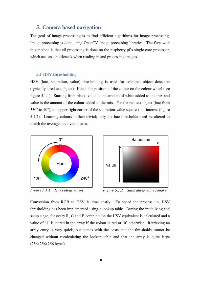
5.1 HSV thresholding HSV (hue, saturation, value) thresholding is used for coloured object detection

(typically a red test object). Hue is the position of the colour on the colour wheel (see

figure 5.1.1). Starting from black, value is the amount of white added to the mix and

value is the amount of the colour added to the mix. For the red test object (hue from

350° to 10°), the upper right corner of the saturation-value square is of interest (figure

5.1.2). Learning colours is then trivial; only the hue thresholds need be altered to

match the average hue over an area.

Figure 5.1.1 Hue colour wheel Figure 5.1.2 Saturation-value square

Conversion from RGB to HSV is time costly. To speed the process up, HSV

thresholding has been implemented using a lookup table. During the initializing and

setup stage, for every R, G and B combination the HSV equivalent is calculated and a

value of ‘1’ is stored in the array if the colour is red or ‘0’ otherwise. Retrieving an

array entry is very quick, but comes with the costs that the thresholds cannot be

changed without recalculating the lookup table and that the array is quite large

(256x256x256 bytes).

20

To offset the large memory cost the colour space has been reduced. Each channel is

mapped from [0,255] down to buckets of [0,7]. This conversion is also done using a

lookup table.

5.2 Single coloured object detection A center of mass type algorithm is used for coloured object detection. The average

position of the red pixels is calculated as the sum of rows or columns of the red pixels

divided by the total number of red pixels. If the number of red pixels is larger than a

certain threshold, a red object is considered as being detected.

The flaw with this algorithm is when more than one red object is present in the frame;

the average is split between the objects. An improvement on is the cam-shift

algorithm [38]. Rather than scanning over the whole frame, only a window is

scanned. Assuming that a red object is present in the frame and moves slow enough

that it does not escape the widow entirely, the center of mass is recalculated and the

window for the next frame is constructed around the new center of mass. That way

the window follows the object.

If the window is of a fixed size, the algorithm is called a mean-shift [38]. For an

adaptive window, the algorithm is a cam-shift (continuously adaptive mean-shift) and,

using the assumption that the object is square, the length and width of the window are

made proportional to area of the object, or the number of pixels detected. In the

implementation of this algorithm on the copter, the window is set to the entire frame

when no objects are detected.

5.3 Coloured object tracking The following program loop was used for tracking a red object (figure 5.3.1). The

copter hovers, rotates on the spot and lowers/raises the gimbal to keep the object in

frame.

21

Figure 5.3.1 Control flow diagram for object tracking

22

6. Results and discussion

6.1 GPS-based navigation Trials  were  done  at  UWA’s  James  oval  over  the  cricket  pitch. As a safety precaution,

no one is to walk under the hexacopter whilst in flight. The cricket pitch was used for

convenience because the grounds people barricad it off to prevent people from

walking on it.

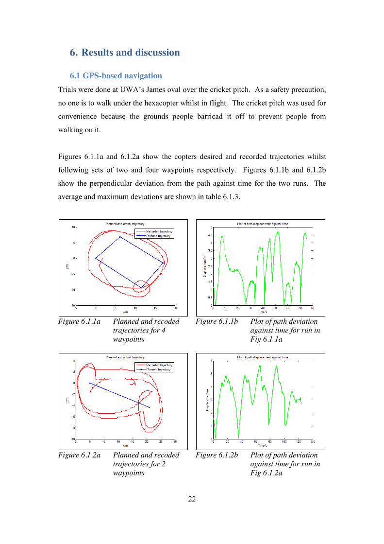
Figures 6.1.1a and 6.1.2a show the copters desired and recorded trajectories whilst

following sets of two and four waypoints respectively. Figures 6.1.1b and 6.1.2b

show the perpendicular deviation from the path against time for the two runs. The

average and maximum deviations are shown in table 6.1.3.

Figure 6.1.1a Planned and recoded

trajectories for 4 waypoints

Figure 6.1.1b Plot of path deviation

against time for run in Fig 6.1.1a

Figure 6.1.2a Planned and recoded

trajectories for 2 waypoints

Figure 6.1.2b Plot of path deviation

against time for run in Fig 6.1.2a

23

Average deviation Maximum deviation

Run 1 2.33 m 4.70 m

Run 2 3.39 m 5.66 m

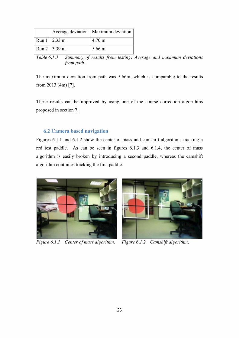
Table 6.1.3 Summary of results from testing: Average and maximum deviations from path.

The maximum deviation from path was 5.66m, which is comparable to the results

from 2013 (4m) [7].

These results can be improved by using one of the course correction algorithms

proposed in section 7.

6.2 Camera based navigation Figures 6.1.1 and 6.1.2 show the center of mass and camshift algorithms tracking a

red test paddle. As can be seen in figures 6.1.3 and 6.1.4, the center of mass

algorithm is easily broken by introducing a second paddle, whereas the camshift

algorithm continues tracking the first paddle.

Figure 6.1.1 Center of mass algorithm.

Figure 6.1.2 Camshift algorithm.

24

Figure 6.1.3 Center of mass algorithm

with second red object introduced.

Figure 6.1.4 Camshift algorithm with

second red object introduced.

The main goal of this part of the project is to increase the efficiency of image

processing. Experiments were conducted as follows: the program was run in isolation

exhaustively and timed how long it took to capture process and display 10000 frames,

and the average frame duration is taken as a measure of efficiency (the shorter, the

more efficient). Frame rate is found by taking the inverse of average frame duration.

Figure 6.2.5 is a comparison of capturing and displaying different resolution images

without any image processing algorithms. Using the smallest resolution (320x240)

produced the best results.

Figure 6.2.5 Frame durations for capturing and displaying images at different

resolutions. No image processing conducted in this set of tests.

25

Figure 6.2.6 is a comparison of the different image processing algorithms proposed in

section 5.2. The resolutions listed are virtual resolutions; resolution was decreased by

skipping pixels when processing without creating a new image. All images are still

captured and displayed at the minimal 320x240 resolution. The algorithm performs

satisfactorily when images are processed at a resolution of 160x120.

Figure 6.2.6 Frame durations for capturing, processing and displaying images. All

images are captured and displayed at 320x240. The resolutions listed are those of the image processing algorithm.

Figure 6.2.7 is a comparison of the image processing whilst being streamed as an

mjpg. All images are captured at a resolution of 320x240 and processed at a

resolution of 160x120. Streaming at 160x120 produced a satisfactory video stream

for viewing on a tablet or smart phone.

26

Figure 6.2.7 Frame durations for capturing, processing and streaming images. All

images are captured at 320x240 and processed at 160x120. The resolutions listed are those of the image stream.

For a reasonable resolution of 320x160, images can be processed using the camshift

algorithm with resolution of 160x120 at a frame rate of up to 26fps. This is a

considerable improvement from 2013 where the maximum frame rate achieved with a

similar algorithm was 8.5fps [7].

This process can also be streamed with a resolution of 160x120 at 9.8fps.

Using the flow program devised in section 5.3, the copter was able to track a red bin

lid moving at slow walking pace (~1kph) for 1.13min, the entire length of the trial.

The video is hosted at:

<https://dl.dropboxusercontent.com/u/68798381/Hex%20Demo.mp4>

6.3 Discussion of practical issues and problems encountered when using the raspberry pi on a hexacopter platform

Several practical issues have arisen when using the current hardware setup. These

range from power to vibration issues.

27

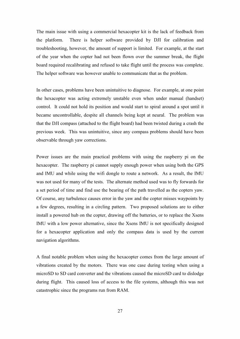
The main issue with using a commercial hexacopter kit is the lack of feedback from

the platform. There is helper software provided by DJI for calibration and

troubleshooting, however, the amount of support is limited. For example, at the start

of the year when the copter had not been flown over the summer break, the flight

board required recalibrating and refused to take flight until the process was complete.

The helper software was however unable to communicate that as the problem.

In other cases, problems have been unintuitive to diagnose. For example, at one point

the hexacopter was acting extremely unstable even when under manual (handset)

control. It could not hold its position and would start to spiral around a spot until it

became uncontrollable, despite all channels being kept at neural. The problem was

that the DJI compass (attached to the flight board) had been twisted during a crash the

previous week. This was unintuitive, since any compass problems should have been

observable through yaw corrections.

Power issues are the main practical problems with using the raspberry pi on the

hexacopter. The raspberry pi cannot supply enough power when using both the GPS

and IMU and while using the wifi dongle to route a network. As a result, the IMU

was not used for many of the tests. The alternate method used was to fly forwards for

a set period of time and find use the bearing of the path travelled as the copters yaw.

Of course, any turbulence causes error in the yaw and the copter misses waypoints by

a few degrees, resulting in a circling pattern. Two proposed solutions are to either

install a powered hub on the copter, drawing off the batteries, or to replace the Xsens

IMU with a low power alternative, since the Xsens IMU is not specifically designed

for a hexacopter application and only the compass data is used by the current

navigation algorithms.

A final notable problem when using the hexacopter comes from the large amount of

vibrations created by the motors. There was one case during testing when using a

microSD to SD card converter and the vibrations caused the microSD card to dislodge

during flight. This caused loss of access to the file systems, although this was not

catastrophic since the programs run from RAM.

28

7. Alternative flight vector methods The following alternate flight vectoring methods were designed and simulated. A

crash late in the project prevented them from being tested.

7.1 Intermediate goal flight vectoring To add course correction capabilities, a number of intermediate goals or path points

are plotted, equally spaced apart and in a line between the previous waypoint and the

last. A path point is counted as reached either if the copter comes within a predefined

distance of the path point, or if the next path point is closer than the current one.

The speed of the flight vector is calculated using a PI controller on distance to the last

path point or next waypoint, same as in 4.2. This was done rather than making speed

proportional to the distance to the closest path point so that the copter does not slow

down for each path point.

The bearing of the flight vector is calculated as a linear combination of bearings to all

unreached path points. Many path points are used to calculate bearing to prevent

oscillations due to the large changes in bearing that occur when the copter is close to

the path point.

Bearings are summed using the weighted average angle formula (adapted from [39]):

𝛼 = 𝑎𝑡𝑎𝑛2(∑ w ∙ sin(𝛼 ) , ∑ w ∙ cos(𝛼 )  )   Eqn 7.1.1

Where n is the number of angles, alpha is the angle and w is the weight for each

angle:

𝑤 = Eqn 7.1.2

The path points are weighted such that each progressive path point is weighted less

than the previous one.

Figure 7.1.1 is a quiver plot showing the flight vectors using the above method and a

P controller only. The main feature is course correction.

29

Figure 7.1.1 Simulation of flight vectors on path using intermediate goal method.

Kp = 1.

7.2 Improved direct flight vectoring In the previous flight vectoring methods, the only one controller is used and the

direction it acts on changes depending on the relative positions waypoints to the

copter. An improved version is proposed by using two orthogonal controllers, one

acting on the N-S axis and another on the E-W axis.

Using the flat earth approximation, lat/lon coordinates are transformed into Cartesian

coordinates  (using  the  copter’s  location as the origin). A waypoint is represented by

vector X0:

𝑋 =𝑥𝑦 Eqn 7.2.1

And the hexacopter is represented by vector H:

𝐻 = 00 Eqn 7.2.2

Therefore the error matrix contains each orthogonal component in separate rows:

𝑒 = 𝐻 − 𝑋 =  −𝑥−𝑦 Eqn 7.2.3

This method is more intuitive, since the memory of the PID controller has a notion of

direction, although this has reduced effect since the copter is flying to a position

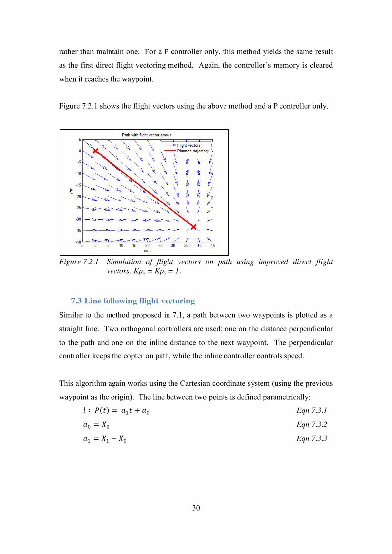
30

rather than maintain one. For a P controller only, this method yields the same result

as  the  first  direct  flight  vectoring  method.    Again,  the  controller’s  memory  is  cleared  

when it reaches the waypoint.

Figure 7.2.1 shows the flight vectors using the above method and a P controller only.

Figure 7.2.1 Simulation of flight vectors on path using improved direct flight

vectors. Kpx = Kpy = 1.

7.3 Line following flight vectoring Similar to the method proposed in 7.1, a path between two waypoints is plotted as a

straight line. Two orthogonal controllers are used; one on the distance perpendicular

to the path and one on the inline distance to the next waypoint. The perpendicular

controller keeps the copter on path, while the inline controller controls speed.

This algorithm again works using the Cartesian coordinate system (using the previous

waypoint as the origin). The line between two points is defined parametrically:

𝑙 ∶  𝑃(𝑡) =  𝑎 𝑡 + 𝑎 Eqn 7.3.1

𝑎 = 𝑋 Eqn 7.3.2

𝑎 = 𝑋 − 𝑋 Eqn 7.3.3

31

Where X1 is the next waypoint and X0 is the previous one. t is only the linking

parameter for the line such that P(t=0) is the start of the line segment and P(t=1) is the

end. t does not represent time.

After plotting the path as a line segment, the next part of this method is projecting the

copter’s  position  onto   the  path.    This   is   taken  as   the  closest  point  on   the   line   to   the  

copter, point P(t1). This is the point where vectors HP(t1) and X1X2 are perpendicular,

and t1 is when the dot product of the two vectors id zero.

𝐻 − 𝑃(𝑡 ) ∙ (𝑋 − 𝑋 ) =  0 Eqn 7.3.4

Working backwards, t1 is found. The side point H is on the line is found using the

sign of determinant:

|𝐻 − 𝑋 ⋮ 𝑋 − 𝑋 | =  𝐻 − 𝑋 𝑋 − 𝑋𝐻 − 𝑋 𝑋 − 𝑋 Eqn 7.3.5

Where the determinant is positive when the H is on the right hand side of line X0X1

and negative when it is on the left.

The perpendicular and inline errors are calculated as:

𝑒 =  −𝑠𝑔𝑛(|𝐻 − 𝑋 ⋮ 𝑋 − 𝑋 |) ∙ ‖𝐻 − 𝑃(𝑡 )‖   Eqn 7.3.6

𝑒 = 𝑠𝑔𝑛(𝑡 − 1) ∙ ‖𝑋 − 𝑃(𝑡 )‖ Eqn 7.3.7

Where the Euclidian norm is used to calculate distances.

The system must then be rotated to the global frame of reference by adding the

following angle to the bearing:

𝜃 = 𝑎𝑡𝑎𝑛2(𝑋 − 𝑋 ,  𝑋 − 𝑋 ) Eqn 7.3.8

Figure 7.3.1 shows the flight vector plot using this method. This system has course

correction like that in section 7.1.

32

Figure 7.3.1 Simulation of flight vectors on path from using line following

algorithm. Kpinline = 1, Kpperpendicular = 1.

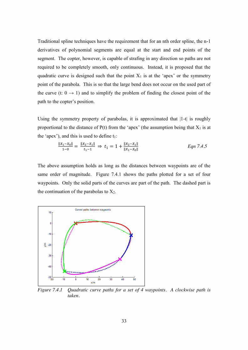
7.4 Curve following The last navigation technique proposed is to follow a simple curve. Curve following

give the added feature that the copter does not need to stop at waypoints; rather it

slows down to make turns and passes smoothly through all waypoints.

The approach taken is extended from the straight-line method above. Paths are made

by interpolating quadratic curves between groups of three waypoints. Higher order

polynomial splines could be used, but are kept to the 2nd order for simplicity.

The parabola is defined parametrically, such that P(t=0) = X0, P(t=1) = X1 and P(t=t1)

= X2 with t1 > 1. The following equations are used [40]:

𝑐 ∶  𝑃(𝑡) =  𝑎 𝑡 + 𝑎 𝑡 + 𝑎 Eqn 7.4.1

𝑎 = 𝑋 Eqn 7.4.2

𝑎 = 𝑋 − 𝑋 − 𝑡 Eqn 7.4.3

𝑎 = ( )  ( )( )

Eqn 7.4.4

Given that X0, X1 and X2 are defined by the waypoints list, the last defining constant

is t1, which is visualized as how much further X2 is along the path from X0 than X1.

In the proposed navigation method, only the portion of the curve from X0 to X1 (t =

[0, 1]) is used. Once X1 is reached, a new curve is calculated using X1, X2 and the

next waypoint.

33

Traditional spline techniques have the requirement that for an nth order spline, the n-1

derivatives of polynomial segments are equal at the start and end points of the

segment. The copter, however, is capable of strafing in any direction so paths are not

required to be completely smooth, only continuous. Instead, it is proposed that the

quadratic curve is designed such that the point X1 is   at   the   ‘apex’  or   the   symmetry  

point of the parabola. This is so that the large bend does not occur on the used part of

the curve (t: 0 →  1) and to simplify the problem of finding the closest point of the

path  to  the  copter’s  position.

Using the symmetry property of parabolas, it is approximated that |1-t| is roughly

proportional  to  the  distance  of  P(t)  from  the  ‘apex’  (the  assumption  being that X1 is at

the  ‘apex’),  and  this  is  used  to  define  t1:

‖ ‖ =   ‖ ‖  ⇒   𝑡 = 1 + ‖ ‖‖ ‖ Eqn 7.4.5

The above assumption holds as long as the distances between waypoints are of the

same order of magnitude. Figure 7.4.1 shows the paths plotted for a set of four

waypoints. Only the solid parts of the curves are part of the path. The dashed part is

the continuation of the parabolas to X2.

Figure 7.4.1 Quadratic curve paths for a set of 4 waypoints. A clockwise path is

taken.

34

Now that the set of rules for planning a path given a set of 3 waypoints has been

defined, the next part of this method is an algorithm for projecting the copters position

onto the path. Based on the assumption that the symmetry point of the parabola is at

t=1, there will only be one point P(t2) with t2<1 where the distance between the

copter’s   location  and   the   curve   is   at   a  minimum.    Therefore   the  closet  point  on   the  

curve to H can be found using a binary search.

The search is restricted to 10 iterations so that the time taken on this step is roughly

constant, and gives t2 to a resolution of 0.001, which translates to a 10m path being

broken up into 1cm sections.

The next part is to find which side of the path the copter lays. A line segment

tangential to the path is extended from point P(t2) to point Q:

𝑄 = 𝑃(𝑡 ) +   ( ) ∙ 1 = 𝑃(𝑡 ) +  2𝑎 𝑡 + 𝑎 Eqn 7.4.6

And equation 7.3.5 is again used to calculate which side of the path the point lays on.

The perpendicular distance is calculated using the Euclidian distance between H and

P(t), same as above:

𝑒 =  −𝑠𝑔𝑛(|𝐻 − 𝑃(𝑡 ) ⋮ 𝑄 − 𝑃(𝑡 )|) ∙ ‖𝐻 − 𝑃(𝑡 )‖   Eqn 7.4.7

Course correction is achieved using a PID controller on the above error.

It is also desired that the copter only slows for waypoints without actually stopping.

The amount it slows down should depend on the angle between waypoints X0X1X2,

i.e. the copter should stop for 180° turns but pass through linear points (0° turn) at full

speed. The speed controller should only begin to take effect when the copter is a

predefined distance from the waypoint. The proposed speed controller equation is set

out below:

𝑠𝑝𝑒𝑒𝑑 =  𝑀𝐴𝑋                                                                                                                                                                         𝑑𝑖𝑠𝑡 > 𝑎𝑝𝑝𝑟𝑜𝑎𝑐ℎ

𝑀𝐴𝑋 + (𝑀𝐴𝑋 −𝑀𝐼𝑁) sin𝜃2   1 −

𝑑𝑖𝑠𝑡𝑎𝑝𝑝𝑟𝑜𝑎𝑐ℎ

𝑜/𝑤

Eqn 7.4.8

35

Where MAX is the maximum speed, MIN is the minimum speed, θ is the angle

between waypoints, dist is the straight line distance to the waypoint and approach is

the predefined distance of approach when the copter is to start slowing for a turn.

Figure 7.4.2 is a plot of the flight vectors on a curved path using the above method.

Points  towards  the  right  of  the  figure  aren’t  populated  with  vectors  since  it  is  assumed  

that the copter is following the new path it plotted after it passed the second waypoint.

Figure 7.4.2 Simulation of flight vectors on path from using curve following

algorithm.

36

8. Conclusions and future work

8.1 Conclusions A multithreaded software system was designed for and implemented on an

autonomous hexacopter. The modular design made this system flexible and

adaptable. The use of mutexs to protect resources across threads makes the design

robust.

The software system was proved to successfully control a hexacopter in autonomous

flight. GPS waypoint navigation was achieved with a path deviation comparable to

last year. Camera image processing streamlined, effectively doubling previous frame

rates. Finally the object tracking was sustained for 1.13 minutes, the entire length of

the test.

This system is currently in use with a variety of simultaneous projects, including field

searching and multiple object tracking, all tied in together with a web based user

interface.

8.2 Future work Modeling of the system is a priority. This will allow for efficient tuning of PID

parameter, the application of state estimation algorithms, namely the EFK, and even

integration with robotics simulators.

Finally, the hexacopter must be fitted with a thermal imaging camera to achieve the

projects original goal: an autonomous application in the agricultural setting.

37

9. Reference list

[1] Global Unmanned Systems Pty Ltd. (2013, 27 October 2014). Mining,

Quarrying & Mineral Exploration. Available: http://www.gus-

uav.com/mining-quarrying-mineral-exploration

[2] CYBERHAWK Innovations Ltd. (2014, 27 October 2014). ROAV inspection

for the offshore oil & gas industry. Available:

http://www.thecyberhawk.com/inspections/offshore-oil-gas/

[3] CYBERHAWK Innovations Ltd. (2014, 27 October 2014). UAV inspection

for the Power and Utility industries. Available:

http://www.thecyberhawk.com/inspections/utilities/

[4] E. B. Knipling, "Physical and physiological basis for the reflectance of visible

and near-infrared radiation from vegetation," Remote Sensing of Environment,

vol. 1, pp. 155-159, 1970.

[5] P. L. Hatfield and P. J. Pinter Jr, "Remote sensing for crop protection," Crop

Protection, vol. 12, pp. 403-413, 1993.

[6] Falcon UAV. (2014, 28 October 2014). Falcon UAV - Increase yeild Reduce

Costs. Available: http://www.falconuav.com.au/

[7] C. Venables, "Mulitrotor Unmanned Aerial Vehicle Autonomous Operation in

an Industrial Environment using On-board Image Processing," B.E. Thesis,

Faculty of Engineering, Computing and Mathematics, University of Western

Australia, 2013.

[8] R. O'Connor, "Developing A Multirotor UAV Platform To Carry Out

Research Into Autonomous Behaviours, Using On-board Image Processing

Techniques," B.E. Thesis, Faculty of Engineering, Computing and

Mathematics, University of Western Australia, 2013.

[9] J. Pestana, I. Mellado-Bataller, J. L. Sanchez-Lopez, C. H. Fu, I. F.

Mondragon, and P. Campoy, "A General Purpose Configurable Controller for

Indoors and Outdoors GPS-Denied Navigation for Multirotor Unmanned

Aerial Vehicles," Journal of Intelligent & Robotic Systems, vol. 73, pp. 387-

400, Jan 2014.

[10] J.-P. Tardif, M. George, M. Laverne, A. Kelly, and A. Stentz, "Vision-aided

Inertial Navigation for Power Line Inspection," in Proc. of the 1st

38

International Conference on Applied Robotics for the Power Industry

(CARPI), 2010, pp. 1-6.

[11] R. Voigt, J. Nikolic, C. Hurzeler, S. Weiss, L. Kneip, and R. Siegwart,

"Robust Embedded Egomotion Estimation," 2011 Ieee/Rsj International

Conference on Intelligent Robots and Systems, pp. 2694-2699, 2011.

[12] T. Tomic, K. Schmid, P. Lutz, A. Domel, M. Kassecker, E. Mair, I. L. Grixa,

F. Ruess, M. Suppa, and D. Burschka, "Toward a Fully Autonomous UAV

Research Platform for Indoor and Outdoor Urban Search and Rescue," Ieee

Robotics & Automation Magazine, vol. 19, pp. 46-56, Sep 2012.

[13] H. Huang, G. M. Hoffmann, S. L. Waslander, and C. J. Tomlin,

"Aerodynamics and control of autonomous quadrotor helicopters in aggressive

maneuvering," in Robotics and Automation, 2009. ICRA'09. IEEE

International Conference on, 2009, pp. 3277-3282.

[14] S. Lupashin, A. Schollig, M. Sherback, and R. D'Andrea, "A Simple Learning

Strategy for High-Speed Quadrocopter Multi-Flips," 2010 Ieee International

Conference on Robotics and Automation (Icra), pp. 1642-1648, 2010.

[15] A. Nemra and N. Aouf, "Robust INS/GPS Sensor Fusion for UAV

Localization Using SDRE Nonlinear Filtering," Ieee Sensors Journal, vol. 10,

pp. 789-798, Apr 2010.

[16] R. Leishman, J. Macdonald, T. McLain, and R. Beard, "Relative navigation

and control of a hexacopter," in Robotics and Automation (ICRA), 2012 IEEE

International Conference on, 2012, pp. 4937-4942.

[17] N. Abdelkrim, N. Aouf, A. Tsourdos, and B. White, "Robust nonlinear

filtering for INS/GPS UAV localization," 2008 Mediterranean Conference on

Control Automation, Vols 1-4, pp. 1090-1097, 2008.

[18] S. Bouabdallah, A. Noth, and R. Siegwart, "PID vs LQ control techniques

applied to an indoor micro quadrotor," in Intelligent Robots and Systems,

2004.(IROS 2004). Proceedings. 2004 IEEE/RSJ International Conference on,

2004, pp. 2451-2456.

[19] G. Welch and G. Bishop, "An introduction to the Kalman filter," Department

of Computer Science, University of North Carolina, 1995.

39

[20] R. Baránek and F. Solc, "Modelling and control of a hexa-copter," in

Carpathian Control Conference (ICCC), 2012 13th International, 2012, pp.

19-23.

[21] DJI. (2014, 28 October 2014). Flame Wheel Arf Kit. Available:

http://www.dji.com/product/flame-wheel-arf

[22] DJI. (2014, 28 October 2014). NAZA-M. Available:

http://www.dji.com/product/naza-m

[23] R. G. Hirst. (2014). ServoBlaster. Available:

https://github.com/richardghirst/PiBits/tree/master/ServoBlaster

[24] Qstarz International Co. Ltd. (2013, 28 October 2014). BT-Q818X XGPS.

Available: http://www.qstarz.com/Products/GPS%20Products/BT-Q818X-

S.htm

[25] G. Henderson. (2014). wiringPi. Available: http://wiringpi.com/

[26] Xsens North America Inc. (n.d., 27 October 2014). MTi - Miniature MEMS

based AHRS. Available: https://www.xsens.com/products/mti/

[27] RS Components Pty Ltd. (n.d., 28 October 2014). CAMERA MODULE.

Available: http://docs-

asia.electrocomponents.com/webdocs/127d/0900766b8127db0a.pdf

[28] E. Valkov. (2014). RaspiCamCV. Available:

https://github.com/robidouille/robidouille/tree/master/raspicam_cv

[29] Swift Navigation Inc. (2014, 27 October 2014). Piksi. Available:

http://www.swiftnav.com/piksi.html

[30] T. H. Drage, "Development of a Navigation Control System for an

Autonomous Formula SAE-Electric Race Car," B.E. Thesis, School of

Electrical, Electronic and Computer Engineering, University of Western

Australia, 2013.

[31] D. DePriest. (n.d., 28 October 2014). NMEA data. Available:

http://www.gpsinformation.org/dale/nmea.htm

[32] opencv dev team. (2014, 28 October 2014). OpenCV 2.4.9.0 documentation.

Available: http://docs.opencv.org/

[33] Ariandy. (2013, 28 October 2014). Streaming OpenCV Output Through

HTTP/Network with MJPEG. Available:

40

http://ariandy1.wordpress.com/2013/04/07/streaming-opencv-output-through-

httpnetwork-with-mjpeg/

[34] M. Grinberg. (2013, 28 October 2014). How to build and run MJPG-Streamer

on the Raspberry Pi. Available: http://blog.miguelgrinberg.com/post/how-to-

build-and-run-mjpg-streamer-on-the-raspberry-pi

[35] a-n-d-r-e-a-s and tom_stoeveken. (2014). MJPG-streamer. Available:

http://sourceforge.net/projects/mjpg-streamer/

[36] B. Chamberlain. (1998, 28 October 2014). Computing distances. Available:

http://www.cs.nyu.edu/visual/home/proj/tiger/gisfaq.html

[37] C. Veness. (2012, 28 October 2014). Calculate distance, bearing and more

between Latitude/Longitude points. Available: http://www.movable-

type.co.uk/scripts/latlong.html

[38] G. R. Bradski, "Real time face and object tracking as a component of a

perceptual user interface," Fourth Ieee Workshop on Applications of Computer

Vision - Wacv'98, Proceedings, pp. 214-219, 1998.

[39] NCSS Statistical Software. (n.d., 28 October 2014). NCSS Circular Data

Analysis. Available: http://www.ncss.com/wp-

content/themes/ncss/pdf/Procedures/NCSS/Circular_Data_Analysis.pdf

[40] A. Salter. (n.d., 28 October 2014). 3. Parametric spline curves. Available:

http://www.doc.ic.ac.uk/~dfg/AndysSplineTutorial/Parametrics.html