Automotive Sketch Processing in C++ with MATLAB Graphic ...

18

Automotive Sketch Processing in C++ with MATLAB Graphic Library

Qiang Li Jilin University

P. R. China

1. Introduction

The purpose of automotive sketch processing is to separate the sketch into patches and

extract the useful information and apply it to assist 2D to 3D transformation. How to extract

the useful information depends on what the resources are, what kinds of information are

needed, and what methods are applied. In sketches, the information may be extracted from

features such as the geometry features, shading, colours and lighting. Geometry features are

the most important because they contain the information to identify and distinguish

between forms. For example, edges can be used to determine the shapes, and areas can be

used to match the size.

This chapter introduces a way to make the automotive sketches ready for 2D to 3D

transformation. Three aspects of problems are discussed including the pre-processing of

sketches outside computer, the processing of pre-processed sketches inside computer, and

the extraction of features. Some of sketch processing algorithms are implemented in C++

using the MATLAB image processing toolbox, Graphic Library and Math Library. Some

have been developed from scratch. The work describe in this chapter is concerned with the

production of a feasible routine, from the point of view of application, which is capable of

dealing with the real world characteristics of automotive sketches. There is no established

method which provides a suitable starting point for the transformation of real automotive

sketches. The combined algorithms, which are discussed in this chapter, have been found to

be useful.

2. A glimpse of the 23D system

A brief set of requirements, from a usability point of view, for 2D to 3D tool can be summaried as follow:

• Can deal with 2D sketches and 3D models.

• Intuitive, simplified and robust.

• Flexible and expandable.

• Compatible with other CAD and CAM systems. Following the above requirements, a prototype of 2D to 3D system, called “23D”, has been implemented to support the novel method of transforming 2D automotive sketches quickly into 3D surface models.

www.intechopen.com

MATLAB – A Ubiquitous Tool for the Practical Engineer

372

2.1 The development environment

The main development language is Microsoft Visual C++® (Ladd, 1996; Seed, 1996; Smith,

1997; Schildt, 1998) with OpenGL® (Kilgard, 1996; Wright & Sweet, 1996; Fosner, 1997;

Silverio et al., 1997; Chin et al., 1998; Segal & Akeley, 2001), MATLAB® C/C++ Math and

Graphics Libraries (MathWorks, 2001). The basic functions and some algorithms are

implemented based on the Open Geometry (Glaeser & Stachel, 1999), MATLAB

optimisation toolbox (MathWorks, 2000), spline toolbox, and image processing toolbox

(MathWorks, 2001), Image Analysis Pro (IaePro) (Matthews, 2002) and Microsoft VisSDK

(The Vision Technology Group, 2000).

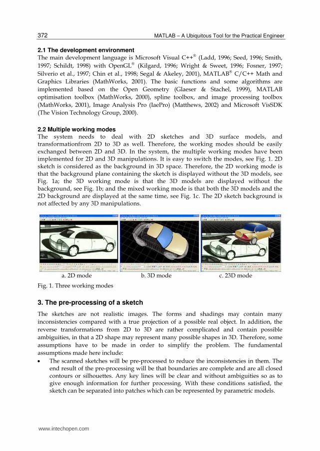
2.2 Multiple working modes The system needs to deal with 2D sketches and 3D surface models, and transformationfrom 2D to 3D as well. Therefore, the working modes should be easily exchanged between 2D and 3D. In the system, the multiple working modes have been implemented for 2D and 3D manipulations. It is easy to switch the modes, see Fig. 1. 2D sketch is considered as the background in 3D space. Therefore, the 2D working mode is that the background plane containing the sketch is displayed without the 3D models, see Fig. 1a; the 3D working mode is that the 3D models are displayed without the background, see Fig. 1b; and the mixed working mode is that both the 3D models and the 2D background are displayed at the same time, see Fig. 1c. The 2D sketch background is not affected by any 3D manipulations.

a. 2D mode b. 3D mode c. 23D mode

Fig. 1. Three working modes

3. The pre-processing of a sketch

The sketches are not realistic images. The forms and shadings may contain many

inconsistencies compared with a true projection of a possible real object. In addition, the

reverse transformations from 2D to 3D are rather complicated and contain possible

ambiguities, in that a 2D shape may represent many possible shapes in 3D. Therefore, some

assumptions have to be made in order to simplify the problem. The fundamental

assumptions made here include:

• The scanned sketches will be pre-processed to reduce the inconsistencies in them. The end result of the pre-processing will be that boundaries are complete and are all closed contours or silhouettes. Any key lines will be clear and without ambiguities so as to give enough information for further processing. With these conditions satisfied, the sketch can be separated into patches which can be represented by parametric models.

www.intechopen.com


373

• Shadings of sketches may be ignored initially, since many techniques of the representations in sketches are not realistic and exact. To derive meaning from them requires psychological interpretation of the intention of the designer, which is beyond the scope of this project.

• Any side, front, rear or top view of automotive model in the sketches is considered to be

orthographic projection, others such as front or rear ¾ perspective views are considered

to be perspective projection.

• Minor details are ignored and allowing concentration on the major ones which establish the essential 3D geometry. It is possible that these could be restored after the basic form has been determined, perhaps using parts from a parts library.

• There is a limit to the exaggeration of forms in a sketch that can be used. Designers

often do use exaggerated geometry to achieve a desired mood. If translated into 3-D,

the resultant model will also contain exaggerated geometry.

• No attempt is made to correct ambiguities of the reverse transformation automatically. These functions are best left for user intervention. The user is likely to be the stylist, who is in a good position to judge which of a number of possibilities best represents the intended vehicle.

As known, not all the sketches are suitable for 3D modelling by the 23D system, but many

do contain the required characteristics. There are many different styles in automotive

sketching, according to the stylist’s personal practice. The information contained varies at

the different conceptual design stages, and is not exactly correct in geometry shape and

projection, because the sketches are not real-world images. Humans can easily interpret the

shape through adding additional information, in the form of prior knowledge of automotive

forms to the sketches and ignoring the faults according to this knowledge. However, the

computer is not as agile as the human. It must have available enough information to create

the shape, which can come from various sources. One approach is to establish a powerful

knowledge database to support the object recognition; another approach is to add the

information before image processing. The former needs larger investment and longer time

to train the computer, and the later needs less investment and is easy to realize. Two

examples of the use of an original sketch as a basis for two well established edge detection

algorithms are shown in Fig. 2c and 2d. The results show that they are difficult to be

interpreted, even by a human. If the results are to be interpretable by a computer program,

significantly more sophisticated processing will be required. Therefore, it is necessary and

feasible to establish some input requirements for the sketches that will be used for 3D

modelling by the method proposed in 23D system, and will form the requirements for the

pre-processing stage. The requirements are relative. The more powerful the pre-processing

method is, the lower the requirements for the interpretive program are. The original

sketches are drawn by stylist, as shown in Fig. 2a and 2e. The results after pre-processing are

shown in Fig. 2b and 2f.

The aim of the pre-processing of sketches is to allow the requirements for the interpretive

program to be met by a greater variety of original sketches. Essentially, the pre-processing

emphasises useful features in the sketches and eliminates useless ones. According to the

analysis of Tingyong Pan (Pan, 2002), the form-lines and form-shadings should be enhanced

and kept, and the non-form-lines and non-form-shadings should be ignored. The vehicle

components should be simplified in details and ambiguities removed. One of the important

www.intechopen.com


374

requirements is that the input sketches should have completed and closed contours or

silhouettes. Any key form-lines should be clear to give enough information to the further

processing. For example, the original sketches (Fig. 2a and 2e) leave some missing and

unclear contours or silhouettes to give an imaginary space. These should be redrawn by

stylists, see the sketches in Fig. 2b and 2f. All the silhouettes are closed and clear. Some

details are ignored such as small lights, highlights, and shadings. The shading information

can be separated from the contour or silhouette information. If the shading information is

important and near realistic, and is within the closed contours, it can be kept. Otherwise, it

should be ignored or further processed to a suitable form. The shadows of the vehicles are

deleted, and the completed silhouettes of wheels are added, which are very important for

the determination of the 3D coordinates. Side elevations, front and rear ¾ perspective views

are the best starting point for system processing.

a. The original sketch b. The pre-processed sketch

(Both sketches by courtesy of Tingyong Pan)

c. Canny method d. Sobel method

e. Canny method f. Sobel method

(Both sketches by courtesy of Tingyong Pan)

Fig. 2. The pre-processing of the sketch

www.intechopen.com


375

It is also important to produce pre-processed sketches with simple patches, which can be

represented using existing parametric models.

Because the features extracted from sketches are currently pixel-based in order to keep the

balance between the speed of processing and the precision of calculation, the suitable size of

input sketches should be carefully considered.

4. Sketch processing

Even though the sketches have been pre-processed before scanning, they also need to be

subject to further image processing before transforming them into 3D. Some basic functions

- such as the adjustment of lightness, hue, and saturation, the exchange from colour to grey

scale and B&W, the erasure of unnecessary areas in the sketch, the separation of form from

non-form line and shading - are used before edge detection and segmentation. To decrease

the size of the dataset and smooth the boundaries, B-spline or NURBS curve fitting to the

outlines are applied. These form-lines are disassembled into spline segments and are used to

build up the patches, which represent the whole surface model.

The original sketches (if applicable) or pre-processed sketches still need to be processed

further in order to obtain a sketch with single pixel edges and closed boundaries, and this

sketch is separated into patches for the downstream processes. Therefore, it is necessary to

investigate a set of efficient image processing algorithms for this application.

4.1 Image mode selection There are many modes for the different purposes of raster image processing including colour and non-colour ones. Some typical colour modes such as RGB (red, green and blue), HSV (hue, saturation and value), HLS (hue, lightness and saturation), and CYMK (cyan, yellow, magenta and black) have been described in the books (Foley et al., 1996; Salomon, 1999). The Adobe Photoshop 6.0 supports colour modes such as RGB, CYMK, Lab (lightness, green-red axis and blue-yellow axis), Indexed Colour, and HSB (hue, saturation and brightness), and non-colour modes such as Greyscale, Multi-channel, Bitmap and Duotone. There are four modes for image displaying and processing supported by the 23D system:

RGB colour, 256 greyscale, 16 greyscale, and black and white (B&W). The internal format is

RGBA colour; therefore the modes can be changed reversibly. The algorithms of greyscale

are different. For example, the Image Analysis Explorer Pro (IaePro) supports three methods

to obtain a greyscale as follows.

0.2125 0.7154 0.0721 Greyscale BT709

0.299 0.587 0.114 Greyscale Y

0.5 0.419 0.081 Greyscale RMY

ij ij ij

ij ij ij ij

ij ij ij

R G B

A R G B

R G B

⎧ + +⎪⎪= + +⎨⎪ + +⎪⎩ (1)

However, for simplification, the transformation from RGB to 256 greyscale used here is an

average algorithm of the colour RGB values (Jain, 1995, pp. 281).

0, , _ 1

0, , _ 1

11 ( )

3i BmpBgr wij ij ij ijj BmpBgr h

A R G B= −= −

= + +AA

(2)

www.intechopen.com


376

Where 1ijA is the greyscale value of a point in image including three components ijR , ijG

and ijB ; BmpBgr_w and BmpBgr_h are the width and the height of sketch in pixels,

respectively. In B&W mode, the two levels are obtained from a point between 0 and 255

to bisect the whole range. A similar function is used in Adobe Photoshop 6.0 (Adobe,

2000).

0, , _ 1

0, , _ 1

0 10 02

1 255 1 255

ij Li BmpBgr wij

L ijj BmpBgr h

A DA

D A= −= −

≤ <⎡ ⎤ ⎡ ⎤= =⎢ ⎥ ⎢ ⎥ ≤ ≤⎣ ⎦ ⎣ ⎦AA

(3)

Where 2ijA is determined by 1ijA , and LD is a threshold to determine a dividing level. The

default of LD is 192, and can be adjusted. The change from 256 greyscale to 16 greyscale is

obtained according to the average rule. A coding scheme proposed in 23D system is that the

values of 16 intervals are increased through adding the value 17 for smoothness and

keeping it spanning to the two ends (0 and 255).

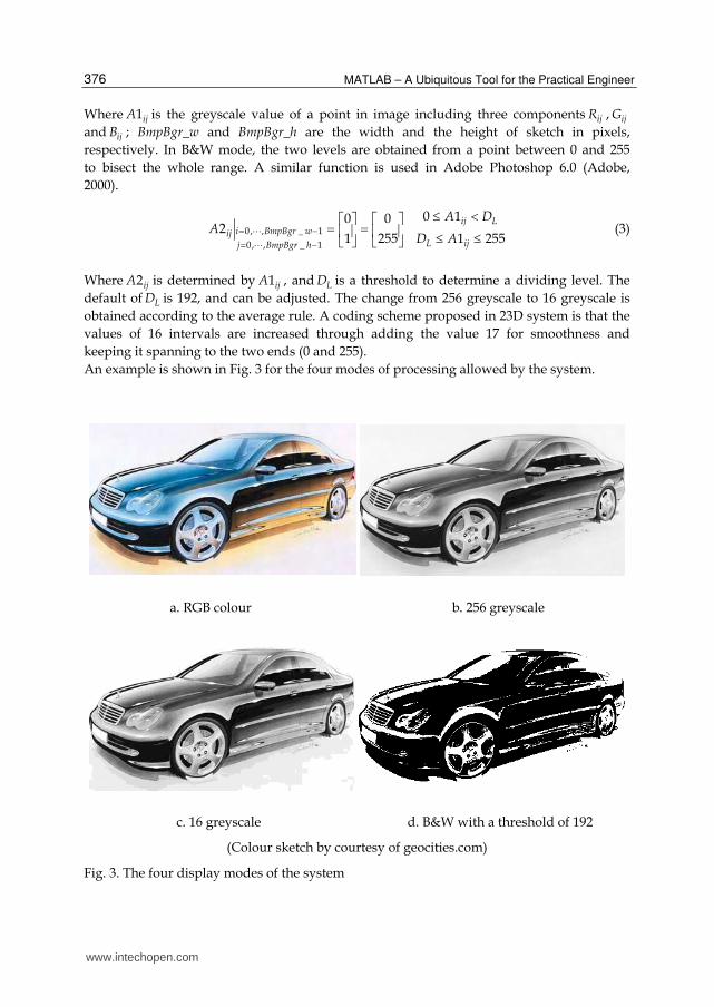
An example is shown in Fig. 3 for the four modes of processing allowed by the system.

a. RGB colour b. 256 greyscale

c. 16 greyscale d. B&W with a threshold of 192

(Colour sketch by courtesy of geocities.com)

Fig. 3. The four display modes of the system

www.intechopen.com


377

0, , _ 1

0, , _ 1

0 0

1 17

2 34

3 51

4 68

5 85

6 102

7 1193

8 136

9 153

10 170

11 187

12 204

13 221

14 238

15 255

i BmpBgr wijj BmpBgr h

A = −= −

⎡ ⎤ ⎡ ⎤⎢ ⎥ ⎢ ⎥⎢ ⎥ ⎢ ⎥⎢ ⎥ ⎢ ⎥⎢ ⎥ ⎢ ⎥⎢ ⎥ ⎢ ⎥⎢ ⎥ ⎢ ⎥⎢ ⎥ ⎢ ⎥⎢ ⎥ ⎢ ⎥⎢ ⎥ ⎢ ⎥⎢ ⎥ ⎢ ⎥⎢ ⎥ ⎢ ⎥= =⎢ ⎥ ⎢ ⎥⎢ ⎥ ⎢ ⎥⎢ ⎥ ⎢ ⎥⎢ ⎥ ⎢ ⎥⎢ ⎥ ⎢ ⎥⎢ ⎥ ⎢ ⎥⎢ ⎥ ⎢ ⎥⎢ ⎥ ⎢ ⎥⎢ ⎥ ⎢⎢ ⎥ ⎢⎢ ⎥ ⎢⎢ ⎥ ⎢⎢ ⎥ ⎢⎣ ⎦ ⎣ ⎦

AA

0 1 16

16 1 32

32 1 48

48 1 64

64 1 80

80 1 96

96 1 112

112 1 128

128 1 144

144 1 160

160 1 176

176 1 192

192 1 208

208 1 224

224 1 240

240 1 255

ij

ij

ij

ij

ij

ij

ij

ij

ij

ij

ij

ij

ij

ij

ij

ij

A

A

A

A

A

A

A

A

A

A

A

A

A

A

A

A

≤ <≤ <≤ <≤ <≤ <≤ <≤ <≤ <≤ <≤ <≤ <≤ <≤ <⎥⎥ ≤ <⎥⎥ ≤ <⎥ ≤ ≤

(4)

4.2 Brightness and contrast adjustment The adjustments of brightness and contrast supply the basic means of image enhancement,

which compensate for the losses caused by imperfect scanning methods. The algorithm from

MATLAB (MathWorks, 2001) imadjust function was used to control the values of RGB

components directly. The brightness bf can be adjusted as follows.

}}

00

0

00

0

(255 ) /1000

(255 ) /100[0,255]

/1000

/100

bb

bb b

bb

b

f b t bf

f t t bf f

f t t bf

f b t b

− ≥⎧ ≥⎪ − <⎪= ∈⎨ ≥⎪ <⎪ <⎩ (5)

Where 0bf is the original value of brightness; t and b are the top and the bottom values of

brightness. They are adjusted by bf , bt t f= + and bb b f= + ; h and l are the highest and the

lowest values among the values of RGB. The differences are defined as dx h l= − , dy t b= − .

They are limited within 0~255.

(255 ) / , 255 255

/ , 0 0

/ , 0 0

( 255) / , 255 255

h l b dx dy t t

h l bdx dy t t

l h tdx dy b b

l h t dx dy b b

= + − = >⎧⎪ = − = <⎪⎨ = − = <⎪⎪ = − − = >⎩ (6)

If the original value 0 0cf ≥ , the contrast cf can be adjusted as

www.intechopen.com


378

0 / 200 [0,255]c c cf f dx f= ∈ (7)

Then h and l should be adjusted as ch h f= − and cl l f= + . Otherwise, the image is not

enhanced. The boundaries should be adjusted again.

0 1

1 1 0 0

0 2 1 0 0

2 2 2 0 0

0.5 / [ ( / )(100 )]

255; 0.5( ), 0.5( )where

0.5 / (255 )

0;

ch x dy k y t k tg arctg dy dx f

h t y y t x h l y t b

l x dy k y b y y k x

l b y y b y y kx

= + ≥ = +⎧ ⎧⎪ ⎪= = < = + = +⎪ ⎪⎨ ⎨= − ≤ = + −⎪ ⎪⎪ ⎪= = > = −⎩ ⎩ (8)

The Gamma value fγ is adjusted according to the original value 0fγ as follow.

( )1.2

0 / 5 [1,10]f f fγ γ γ= ∈ (9)

Therefore, the RGB values of each pixel can be calculated as follow.

( )( )( )

( )/( )

( )/( )

( )/( )

( )

0, , _ 1( )

0, , _ 1

( )

ij

ij

ij

R l h l

ijG l h l

ij

B l h lij

b t b CR

i BmpBgr wG b t b C

j BmpBgr hB

b t b C

γγγ

− −− −− −

⎡ ⎤+ −⎡ ⎤ ⎢ ⎥⎢ ⎥ = −⎢ ⎥= + −⎢ ⎥ ⎢ ⎥ = −⎢ ⎥ ⎢ ⎥⎢ ⎥ ⎢ ⎥⎣ ⎦ + −⎣ ⎦

AA (10)

The dialog window and examples are shown in Fig. 4. The range of the sliders is 100± .

4.3 Edge detection Many algorithms for edge detection have been developed for different image resources.

Because the sketches are not the real-world images and can be pre-processed before

imported into the system, the edge detection is just a simple routine to quickly find the

necessary points for the further processing. Therefore some basic and common algorithms

are implemented into the system including Sobel, Prewitt, Roberts, Canny, Zerocross, Direct

and Sobel+. The system was built using the MATLAB C++ Math Library and the Graphics

Library (MathWorks, 2000). The dialog window is shown in Fig.5, which is similar to the

MATLAB find edges function.

Some examples are shown in Fig. 6 and Fig. 7. In most cases, the algorithms from the

MATLAB edge functions can give good results for original sketches, shown in Fig. 6.

However, they give poor results on pre-processed sketches, shown in Fig. 7b and Fig. 7d.

The pre-processed sketches are composed of sets of dense and thick strokes coming from a

quick expression of the edges according to the original sketches. Therefore, a hybrid

algorithm, Direct, is proposed to deal with such styled sketches.

The idea comes from a demo – Region Labelling of Steel Grains – in the MATLAB image

processing toolbox. Two binary images are obtained from pre-processed sketches by using

low and high thresholds. The edge points from low threshold image are used to delete the

same points from high threshold image. The left edge points from the high threshold image

are considered as the edges. In this way minor regions caused by strokes are deleted. The

result is shown in Fig. 7c produce from a thick edge image.

www.intechopen.com


379

a. Original Sketch b. fb = -33%

c. fc = 45% d. fb = 34%, fc = -50%

e. fγ = 25% f. The dialog window designed

Fig. 4. The samples of the brightness and contrast adjustment

Fig. 5. The dialog window of Find Edges function

www.intechopen.com


380

a. Original sketch b. Sobel algorithm, threshold = 0.13

c. Canny algorithm, threshold = 0.15-1.0 d. LoG algorithm, threshold = 0.007

(Original sketch by courtesy of Cor Steenstra, Foresee Car Design)

Fig. 6. Edge detection of the original colour sketch with the different algorithms

a. Pre-processing sketch b. Roberts algorithm, threshold = 0.1

c. Hybrid algorithm d. Sobel+ algorithm

Fig. 7. Edge detection of the pre-processed sketch

www.intechopen.com


381

To obtain a satisfactory result, it is crucial to select a suitable threshold for edge detection. However, some problems are still left such as thick edges, double edges and broken edges which cause unclosed boundaries, and small ‘spurs’ or ‘prickles’. Therefore, further processing is needed to eliminate these problems.

4.4 Edge morphing Edge morphing can further refine the image obtained from edge detection. This function is implemented using the MATLAB bwmorph function including the method Bothat, Bridge, Clean, Close, Diag, Dilate, Erode, Fill, Hbreak, Majority, Open, Remove, Shrink, Skel, Spur, Thicken, Thin and Tophat, as shown in Fig. 8. It can apply specific morphological operations to the binary image. Repeated application of these operations may be necessary. Infinite means that Times are determined by the methods automatically.

Fig. 8. The dialog window of Edge Morphing function

a. Thin operation (Times = 7) b. Debubble algorithm

Fig. 9. Edge thins and debubbles (Please refer to Fig. 7c)

When the edges are not single pixels such as the ones shown in Fig. 7c, edge morphing should be applied. The result after the seven applications of the thin operation is shown in Fig. 9a. The edges become the single pixels, but with some small holes and spurs. This is still not a satisfactory starting point for the transformation. The bubbles and spurs must be eliminated.

4.5 Debubble – a hybrid algorithm It has not proved to be possible to obtain the required result using a single method. Different hybrid methods have been applied to achieve a good result. Here is a hybrid algorithm proposed in this research to perform an operation of deleting the small holes and spurs, such as shown in Fig. 9a. The algorithm entitled Debubble, shown in Fig. 10, applies

www.intechopen.com


382

firstly the Bwlabel algorithm in MATLAB to find the small bubbles (holes), which are determined by the bubble size parameter. Once the small bubbles are found, they are filled into solid areas. Then the Skel and Spur algorithms are applied to obtain the single pixel edges. The actual bubble size is the percentage of the maximum size in pixels, which is compared with the image size in pixels. For example, to obtain the result in Fig. 9b, the

actual bubble size is 165, and the image size is 524288 (1024×512). This is just 0.0315% of the image size – very small bubbles! In this case, all the bubbles those are smaller than 165 are deleted. The result shown in Fig. 9b is quite acceptable. Using the Direct, Thin, and Debubble algorithms for the pre-processed sketches can give a good result.

Fig. 10. The dialog window of Debubble function

4.6 Edge refinement Once satisfactory edges are obtained, the image is ready for segmentation. However, there are still anomalies that must be handled. For example, see the case in Fig. 11a, the crossing point of the three patches is not unique. This produces three crossing points. In order to delete this small error, the edge points must be checked and refined.

a. Crossing points are not unique b. Unique crossing point

Fig. 11. Crossing point searching

An algorithm is proposed here to perform this operation. It is described as follow:

• Every point is checked in the whole image.

• If it is an edge point, a counter is set with initial value of zero. The point is the current point.

• The eight neighbours of the current point are checked one by one from 0 to 7, see Fig. 12a.

• Once a neighbour point is edge point, the counter is increased by one.

• The current neighbour point is anomaly point, once the counter reaches three within the eight neighbours.

www.intechopen.com


383

• The last current neighbour is deleted.

3 2 1 5 1 4

4 ● 0 a 2 ● 0 b

5 6 7 6 3 7

Fig. 12. Eight-neighbour graph

The result is shown in Fig. 11b. Now the three patches share the same single pixel boundaries and have a unique crossing point.

4.7 Patch segmentation with colours It is easy to separate an image with closed boundaries into patches by applying the MATLAB Bwlabel function, and it can then be displayed with the different colour maps. The Pseudo Colormap includes Autumn, Bone, Colorcube, Cool, Copper, Flag, Gray, Hot, HSV, Jet, Lines, Pink, Prism, Spring, Summer, White and Winter, as shown in Fig. 13. The label 0 is assigned to the boundaries between the patches. Label 1 is assigned to the background and used as the silhouette of the whole vehicle. From label 2 onwards, they are assigned to the patches which form the surfaces of the vehicle. After labelling, a pseudo colour map is added for separating the patches. The labelled image is shown in Fig. 14.

Fig. 13. The dialog window of Patch Segmentation function

a. Labelled sketch b. Multiple Selection of patches

Fig. 14. The sketch after segmentation

www.intechopen.com


384

As well as the labelling and colour mapping, some other tasks are performed at the same time, such as finding out the start points of each patch on the boundary and the maximum rectangles containing each patch, initialising the boundary node data and searching all the sequential nodes and the crossing points on the boundary of each patch, and calculating the areas and centres of patches.

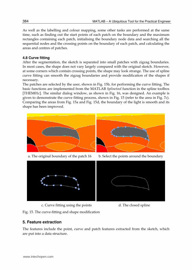
4.8 Curve fitting After the segmentation, the sketch is separated into small patches with zigzag boundaries. In most cases, the shape does not vary largely compared with the original sketch. However, at some corners which contain crossing points, the shape may look strange. The use of spline curve fitting can smooth the zigzag boundaries and provide modification of the shapes if necessary. The patches are selected by the user, shown in Fig. 15b, for performing the curve fitting. The basic functions are implemented from the MATLAB Splinetool function in the spline toolbox [THEM01c]. The similar dialog window, as shown in Fig. 16, was designed. An example is given to demonstrate the curve fitting process, shown in Fig. 15 (refer to the area in Fig. 7c). Comparing the areas from Fig. 15a and Fig. 15d, the boundary of the light is smooth and its shape has been improved.

a. The original boundary of the patch 16 b. Select the points around the boundary

c. Curve fitting using the points d. The closed spline

Fig. 15. The curve-fitting and shape modification

5. Feature extraction

The features include the point, curve and patch features extracted from the sketch, which

are put into a data structure.

www.intechopen.com


385

Fig. 16. The dialog window of Curve Fitting function

5.1 Data structure for sketch The points after labelling contain a lot of information for further processing and analysis. Therefore, it is important to establish an efficient data management system. A proposed sketch structure is shown in Fig. 17. The basic unit is a single point, a set of points presents a curve, a close curve or several curves stands for a patch, all the patches make a vehicle.

Fig. 17. Sketch data structure

5.2 Point features After labelling, the sketch becomes a two-dimensional integer array. Zero stands for boundaries as known, but it is necessary to find out which patch it belongs to. They are just the separate edge points with the value of zero at the moment, nothing else. They should be reorganised to useful data. As the basic unit from data structure, 2D point contains three basic features – the coordinates {x, y}, attributes (crosspoint, selected, breakpoint), and links (previous point, next point).

Sketch

Patch Patch Patch

Point Point Point

Curve Curve Curve Curve Curve Curve

www.intechopen.com


386

After labelling, each boundary point has at least two different neighbours. If more than two, the point is a crosspoint. If the point is selected for spline fitting, the selected attribute is true. If the point is used for breaking whole boundary into pieces, the breakpoint attribute is true. The links like a chain join the separated points into a sequential structure. The extraction of point features follows the other feature calculations. A simple algorithm searching related neighbours is developed as follows

• Assume that the current point is an edge point. The eight neighbours of the current point are checked one by one from 0 to 7, see Fig. 12a.

• Once a neighbour is not an edge point, the first related neighbour is found and saved.

• Carry on searching, any different neighbour will be saved until all neighbours are checked. Return the number of related neighbours and an array containing the different neighbours.

• If the number of related neighbours is greater than two, the current point is a breakpoint.

5.3 Curve features A set of edge points around a patch make a closed curve. Each closed boundary may have more than one curve segments, i.e., each segment has its own point set. The point sets may be sparse for curve fitting in order to reduce the size of data and obtain a precise representation of the sketch. The following features need to be extracted in a curve:

• Number of points, and the coordinates of each point (values)

• Number of breakpoints if a closed boundary is broken down to several segments.

• The first point and the last point, if the last point is equal to the first point, it is a closed boundary.

• Curve type, either the outer silhouette curve or the internal curve If using spline fitting to present a curve, the following features need to be extracted.

• Number of selected points for curve fitting

• Fitting method selected.

• End conditions.

• If the point doesn’t belong to the original boundary point, a changed tag is given.

• If displaying a spline, a view tag is given.

• If displaying marks on each node, a mark tag is given. A searching algorithm of boundary curve point setting is based on single pixel has been developed as follows.

• If a point is an edge point and one of its neighbours is the patch, the edge point belongs to the patch.

• The first edge point is the start point of boundary curve, and it becomes the current point, previous point 1 and previous point 2.

• Check the eight neighbours of the current point using the graph in Fig. 12b.

• Once a neighbour point is the edge point and it belongs to the patch, and it is not the previous point 1 and 2, it is a new edge point. Add it to the curve.

• The new edge point becomes the current point. Repeat the same procedure from beginning, until the point is equal to the first point.

In the algorithm, two previous points are used to determine the direction of processing. Using the neighbour graph in Fig. 12b will obtain slightly smoother curves than using the one in Fig. 12a.

www.intechopen.com


387

5.4 Patch features Several curve segments are joined together into a closed curve to form a patch. The following features can be extracted.

• The patch serial number, i.e. the label number

• The colour and the title of patch

• If selected for display or processing, a selected tag is given

• The minimum rectangle containing the patch

• The area and centre of the area of patch, the area value is the number of points within the patch. The centre is the sum of coordinates divided by the area.

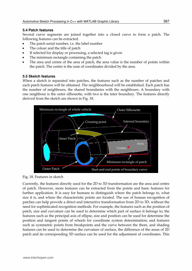
5.5 Sketch features When a sketch is separated into patches, the features such as the number of patches and each patch features will be obtained. The neighbourhood will be established. Each patch has the number of neighbours, the shared boundaries with the neighbours. A boundary with one neighbour is the outer silhouette, with two is the inter boundary. The features directly derived from the sketch are shown in Fig. 18.

Fig. 18. Features in sketch

Currently, the features directly used for the 2D to 3D transformation are the area and centre

of patch. However, more features can be extracted from the points and basic features for

further application. It is easy for humans to distinguish where the patch belongs to, what

size it is, and where the characteristic points are located. The use of human recognition of

patches can help provide a direct and interactive transformation from 2D to 3D, without the

need for sophisticated recognition methods. For example, the features such as the position of

patch, size and curvature can be used to determine which part of surface it belongs to; the

features such as the principal axis of ellipse, size and position can be used for determine the

position and tangent points of wheels for coordinate system determination; and features

such as symmetric points from breakpoints and the curve between the them, and shading

features can be used to determine the curvature of surface, the difference of the areas of 2D

patch and its corresponding 3D surface can be used for the adjustment of coordinates. This

Minimum rectangle of patch

Minimum rectangle of whole vehicle

Internal boundary Crossing point

Start and end points of boundary curve

Centre

Area

Inner Patch

Outer Patch

Outer Silhouette

www.intechopen.com


388

can all be done in a straightforward manner so long as the patch is correctly identified,

which is most readily done by human intervention (although an automated, possibly

artificial intelligence based method for this may be feasible, but is outside the scope of this

research).

6. Implementation of MATLAB functions

As mentioned above, the 23D system has been implemented the MATLAB functions.

Differing from the proposed method of MATLAB implementation, our method was to apply

directly the kernel part of their functions. At first, the MATLAB *.m files were converted

into *h and *.cpp files of C++. Then, it was to extract the kernel part of the function, and to

add them into the 23D system. It was necessary to implement all the related functions.

Therefore, no *.dll or *.lib files of MATLAB were used. This method is quite simple and easy

to change or enhance the implemented functions.

7. Conclusion

The approach here has been to reduce the problem of pre-processing of the sketch into a

number of separate stages, each of which refines or extracts a particular piece of information

embodied in the sketch. Some conclusions are summarized below:

• The pre-processing of sketches plays an important role for the input sketches. The more precise the sketches are, the easier the sketch processing is. Pre-processing can be used to translate ‘imprecise’ sketches to more ‘precise’ ones, providing a better starting point for the transformation process. This approach allows the system to deal with sketches that have roughly closed boundaries, in turn allowing easier separation into patches.

• For the pre-processed sketches, the related processing algorithms have been investigated in order to obtain the separated patches with single-pixel and closed boundary, which are ready for the 2D to 3D transformation. Facing the specific sketches, some existing or new algorithms and new hybrid algorithms have been proposed.

• Some basic features are extracted from the patches to present points, curves and patches. They are listed below.

• The boundary points

• The relationships of the patches

• The minimum rectangle containing the patches

• The start and end points for each boundary

• The areas and geometric centres of the patches

• The attributes of the points whether they are the selected, break or crossing points Related searching and calculating algorithms have been also developed. Some features are

discussed and may be applied in further research.

• The sketch processing and feature extraction depend on the raster data. Therefore, the method is device dependent. The inherent error is one pixel. Increasing the sketch size can reduce error. But the important issue is the quality of the input sketch. A good sketch will produce significantly better results.

• Curve fitting supplies an additional way to improve the patches. Through the selection and modification of the edge points, the shapes of the patches can be smoothed or even

www.intechopen.com


389

be changed in some places. This process allows resolution of a further set of imperfections in the original sketch.

• Direct implementation of MATLAB functions is a feasible way to enhance 23D system functions.

8. Acknowledgment

I would like to take this opportunity to express my special thanks to my supervisor, Dr. R. M. Newman, for his invaluable guidance, supports and helps in the research project. Many thanks also go to the other members of the research group, Prof. M. Tovey, C. S. Porter and J. Tabor, for their ideas, supports and helps in the research project, and T. Y. Pan for his exchanging the information, ideas and supports with me. I am grateful to a number of staffs and students in the MIS, especial in the CTAC, who have discussed with me on my project and have given me lots of support and help, especially to Prof. Keith. J. Burnham, Mrs. A. Todman, and Miss Y. Xie.

9. References

Adobe System Incorporated. (2000). Adobe® Photoshop® 6.0 user guide for Windows® and Macintosh, Adobe System Incorporated, 90024592

Chin, N.; Frazier, C. & Ho, P. (1998). The OpenGL® Graphics System Utility Library. version 1.3, ed. Leech, J.

Foley, J. D.; van Dam, A. & Feiner, S. K. (1996), Computer graphics: principles and practice, 2nd ed. in C, Addison-Wesley Publishing Company, Inc. ISBN 0-201-84840-6

Fosner, R. (1997). OpenGLTM Programming for Windows® 95 and Windows NTTM. Addison-Wesley, ISBN 0-201-40709-4

Glaeser, G. & Stachel, H. (1999). Open Geometry: OpenGL® + Advanced Geometry. Springer-Verlag New York, Inc., ISBN 0-387-98599-9

Kilgard, M. J. (1996). The OpenGL Utility Toolkit (GLUT) Programming Interface. API version 3, Silicon Graphics, Inc.

Ladd, S. R. (1996). C++ Templates and Tools. 2nd ed., M&T Books, ISBN 1-55851-465-1 Matthews, J. (2002). Image Analysis Explorer Pro. version 1.01, http://www.gener-

ation5.org/iae.shtml Pan, T. Y. (2002). Identification of 3D Information from 2D Sketches in Automotive Design,

MPhil paper, School of Art and Design, Coventry University Salomon, D. (1999), Computer graphics and geometric modelling, Springer-Verlag New

York, Inc. ISBN 0-387-98682-0 Schildt, H. (1998). C++ from the Ground up. 2nd ed., Osborne/McGraw-Hill, ISBN 0-07-

882405-2 Seed, G. H. (1996). An Introduction to Object-oriented Programming in C++: With

Applications in Computer Graphics. Springe-Verlag London Ltd., ISBN 3-540-76042-3

Segal, M. & Akeley, K. (2001). The OpenGL® Graphics System: A Specification. version 1.3, ed. Leech, J.

Silverio, C. J.; Fryer, B. & Hartman, J. (1997). OpenGL® Porting Guide. rev. Kempf, R. ed. Cary, C., Silicon Graphics, Inc.

www.intechopen.com


390

Smith, J. T. (1997). C++ Toolkit for Scientists and Engineers. International Thomson Computer Press, ISBN 1-85032-889-7

The MathWorks, Inc. (2000). MATLAB® C/C++ Graphics Library – The Language of Technical Computing - User’s Guide, version 2

The MathWorks, Inc. (2000). MATLAB® C Math Library – The Language of Technical Computing - User’s Guide, version 2

The MathWorks, Inc. 2000, “MATLAB® C++ Math Library – The Language of Technical Computing - User’s Guide”, version 2, The MathWorks, Inc.

The MathWorks, Inc. 2001, “MATLAB® Compiler – The Language of Technical Computing - User’s Guide”, version 2, The MathWorks, Inc.

The MathWorks Inc. (2001). MATLAB® The Image Processing Toolbox User's Guide, version 3

The MathWorks, Inc. (2001). Spline Toolbox for Use with MATLAB® - User’s Guide, version 3.

The Vision Technology Group, Microsoft Research. (2000). The Microsoft Vision SDK. version 1.2, [email protected].

Wright, R. S. & Sweet M. (1996). OpenGL Superbible: The Complete Guide to OpenGL Programming for Windows NT and Windows 95. The Waite Group, Inc.

www.intechopen.com

MATLAB - A Ubiquitous Tool for the Practical EngineerEdited by Prof. Clara Ionescu

ISBN 978-953-307-907-3Hard cover, 564 pagesPublisher InTechPublished online 13, October, 2011Published in print edition October, 2011

InTech EuropeUniversity Campus STeP Ri Slavka Krautzeka 83/A 51000 Rijeka, Croatia Phone: +385 (51) 770 447 Fax: +385 (51) 686 166www.intechopen.com

InTech ChinaUnit 405, Office Block, Hotel Equatorial Shanghai No.65, Yan An Road (West), Shanghai, 200040, China

Phone: +86-21-62489820 Fax: +86-21-62489821

A well-known statement says that the PID controller is the â€œbread and butterâ€ of the control engineer. Thisis indeed true, from a scientific standpoint. However, nowadays, in the era of computer science, when thepaper and pencil have been replaced by the keyboard and the display of computers, one may equally say thatMATLAB is the â€œbreadâ€ in the above statement. MATLAB has became a de facto tool for the modernsystem engineer. This book is written for both engineering students, as well as for practicing engineers. Thewide range of applications in which MATLAB is the working framework, shows that it is a powerful,comprehensive and easy-to-use environment for performing technical computations. The book includesvarious excellent applications in which MATLAB is employed: from pure algebraic computations to dataacquisition in real-life experiments, from control strategies to image processing algorithms, from graphical userinterface design for educational purposes to Simulink embedded systems.

How to referenceIn order to correctly reference this scholarly work, feel free to copy and paste the following:

Qiang Li (2011). Automotive Sketch Processing in C++ with MATLAB Graphic Library, MATLAB - A UbiquitousTool for the Practical Engineer, Prof. Clara Ionescu (Ed.), ISBN: 978-953-307-907-3, InTech, Available from:http://www.intechopen.com/books/matlab-a-ubiquitous-tool-for-the-practical-engineer/automotive-sketch-processing-in-c-with-matlab-graphic-library

© 2011 The Author(s). Licensee IntechOpen. This is an open access articledistributed under the terms of the Creative Commons Attribution 3.0License, which permits unrestricted use, distribution, and reproduction inany medium, provided the original work is properly cited.

http://creativecommons.org/licenses/by/3.0

Automotive Sketch Processing in C++ with MATLAB Graphic ...

Documents

Transcript of Automotive Sketch Processing in C++ with MATLAB Graphic ...