Automating Wrong-Way Driving Detection Using Existing CCTV ...
50
Automating Wrong-Way Driving Detection Using Existing CCTV Cameras Final Report December 2020 Sponsored by Iowa Department of Transportation (InTrans Project 18-677)
Transcript of Automating Wrong-Way Driving Detection Using Existing CCTV ...

Automating Wrong-Way Driving Detection Using Existing CCTV CamerasFinal ReportDecember 2020
Sponsored byIowa Department of Transportation(InTrans Project 18-677)

About InTrans and CTREThe mission of the Institute for Transportation (InTrans) and Center for Transportation Research and Education (CTRE) at Iowa State University is to develop and implement innovative methods, materials, and technologies for improving transportation efficiency, safety, reliability, and sustainability while improving the learning environment of students, faculty, and staff in transportation-related fields.
Iowa State University Nondiscrimination Statement Iowa State University does not discriminate on the basis of race, color, age, ethnicity, religion, national origin, pregnancy, sexual orientation, gender identity, genetic information, sex, marital status, disability, or status as a US veteran. Inquiries regarding nondiscrimination policies may be directed to the Office of Equal Opportunity, 3410 Beardshear Hall, 515 Morrill Road, Ames, Iowa 50011, telephone: 515-294-7612, hotline: 515-294-1222, email: [email protected].
Disclaimer NoticeThe contents of this report reflect the views of the authors, who are responsible for the facts and the accuracy of the information presented herein. The opinions, findings and conclusions expressed in this publication are those of the authors and not necessarily those of the sponsors.
The sponsors assume no liability for the contents or use of the information contained in this document. This report does not constitute a standard, specification, or regulation.
The sponsors do not endorse products or manufacturers. Trademarks or manufacturers’ names appear in this report only because they are considered essential to the objective of the document.
Iowa DOT Statements Federal and state laws prohibit employment and/or public accommodation discrimination on the basis of age, color, creed, disability, gender identity, national origin, pregnancy, race, religion, sex, sexual orientation or veteran’s status. If you believe you have been discriminated against, please contact the Iowa Civil Rights Commission at 800-457-4416 or the Iowa Department of Transportation affirmative action officer. If you need accommodations because of a disability to access the Iowa Department of Transportation’s services, contact the agency’s affirmative action officer at 800-262-0003.
The preparation of this report was financed in part through funds provided by the Iowa Department of Transportation through its “Second Revised Agreement for the Management of Research Conducted by Iowa State University for the Iowa Department of Transportation” and its amendments.
The opinions, findings, and conclusions expressed in this publication are those of the authors and not necessarily those of the Iowa Department of Transportation.

Technical Report Documentation Page
1. Report No. 2. Government Accession No. 3. Recipient’s Catalog No.
InTrans Project 18-677
4. Title and Subtitle 5. Report Date
Automating Wrong-Way Driving Detection Using Existing CCTV Cameras December 2020
6. Performing Organization Code
7. Author(s) 8. Performing Organization Report No.
Arya Ketabchi Haghighat (orcid.org/0000-0003-1643-3575), Tongge Huang
(orcid.org/0000-0002-5534-4623), and Anuj Sharma (orcid.org/0000-0001-
5929-5120)
InTrans Project 18-677
9. Performing Organization Name and Address 10. Work Unit No. (TRAIS)
Center for Transportation Research and Education
Iowa State University
2711 South Loop Drive, Suite 4700
Ames, IA 50010-8664
11. Contract or Grant No.
12. Sponsoring Organization Name and Address 13. Type of Report and Period Covered
Iowa Department of Transportation
800 Lincoln Way
Ames, IA 50010
Final Report
14. Sponsoring Agency Code
TSIP
15. Supplementary Notes
Visit www.intrans.iastate.edu for color pdfs of this and other research reports.
16. Abstract
The goal of this project was to detect wrong-way driving using only closed circuit television (CCTV) camera data on a real-time
basis with no need to manually pre-calibrate the camera. Based on this goal, a deep learning model was implemented to detect
and track vehicles, and a machine learning model was trained to classify the road into different directions and extract vehicle
properties for further comparisons.
The objective of this project was to detect wrong-way driving on Iowa highways in 10 different locations. When wrong-way
driving was detected, the system would record the violation scene and send the video file via email to any recipient in charge of
appropriate reactions for the event.
This report covers the background and methodology for the work and the models and modules implemented to compare them to
one another. The Conclusions and Key Findings chapter provides a brief summary of the work and the findings. The final
chapter, Implementation Recommendations Based on Cloud Computing for the Future, includes a discussion of costs and
requirements, along with an economic analysis and future computing suggestions.
17. Key Words 18. Distribution Statement
intelligent transportation systems—wrong-way driving—WWD detection No restrictions.
19. Security Classification (of this
report)
20. Security Classification (of this
page)
21. No. of Pages 22. Price
Unclassified. Unclassified.
46 NA
Form DOT F 1700.7 (8-72) Reproduction of completed page authorized


AUTOMATING WRONG-WAY DRIVING
DETECTION USING EXISTING CCTV CAMERAS
Final Report
December 2020
Principal Investigator
Anuj Sharma, Research Scientist and Leader
Center for Transportation Research and Education, Iowa State University
Research Assistants
Arya Ketabchi Haghighat and Tongge Huang
Authors
Arya Ketabchi Haghighat, Tongge Huang, and Anuj Sharma
Sponsored by
Iowa Department of Transportation
Preparation of this report was financed in part
through funds provided by the Iowa Department of Transportation
through its Research Management Agreement with the
Institute for Transportation
(InTrans Project 18-677)
A report from
Institute for Transportation
Iowa State University
2711 South Loop Drive, Suite 4700
Ames, IA 50010-8664
Phone: 515-294-8103 / Fax: 515-294-0467
www.intrans.iastate.edu


v
TABLE OF CONTENTS
ACKNOWLEDGMENTS ............................................................................................................ vii
EXECUTIVE SUMMARY ........................................................................................................... ix
1 INTRODUCTION, LITERATURE REVIEW, AND BACKGROUND .....................................1
1.1 Goal and Scope ..............................................................................................................5 1.2 Objective and Requirements ..........................................................................................5 1.3 Report Organization .......................................................................................................6
2 PROPOSED METHODS ..............................................................................................................7
2.1 Methodology ..................................................................................................................7
2.1 Structure and Modules ...................................................................................................9
3 EXPERIMENT AND RESULTS ...............................................................................................20
3.1 Calibration....................................................................................................................20
3.2 Results and Discussion ................................................................................................25
4 CONCLUSIONS AND KEY FINDINGS ..................................................................................29
5 IMPLEMENTATION RECOMMENDATIONS BASED ON CLOUD COMPUTING
FOR THE FUTURE .........................................................................................................30
REFERENCES ..............................................................................................................................33

vi
LIST OF FIGURES
Figure 1.1. Implemented passive mechanisms to inform driver to prevent wrong-way
driving: wrong-way signs (top) and in-pavement warnings (bottom) ............................2 Figure 1.2. Implemented sensors to detect wrong-way driving: radar (top), fusion of
camera and radar (middle), and electromagnetic sensors embedded in the
pavement (bottom) ..........................................................................................................3 Figure 2.1. Flow of the fully automated wrong-way driving detection system when
YOLOv3 acts as the detector with SORT as the tracker .................................................9 Figure 2.2. Flow of the fully automated wrong-way driving detection system when
DeepStream produces detection and tracking results ...................................................10 Figure 2.3. Darknet-53 structure ....................................................................................................11 Figure 2.4. Detected vehicles by YOLO ........................................................................................12 Figure 2.5. Tracked vehicles by SORT, results, and losing tracklets ............................................13 Figure 2.6. NVIDIA DeepStream perception module architecture ...............................................14 Figure 2.7. Sample output from DeepStream model where DeepStream does both vehicle
detection and vehicle tracking .......................................................................................15 Figure 2.8. DeepStream with Apache analysis module architecture .............................................16 Figure 2.9. Result of label allocation to each grid using Gaussian mixture model and
classification using SVM with camera field of view (top), Gaussian mixture
model results (bottom left), and SVM results (bottom right)........................................17 Figure 2.10. Result of text recognition module .............................................................................19 Figure 3.1. Result of road side classification for different traffic volumes ...................................21 Figure 3.2. How the road is divided into two different roadside ...................................................22 Figure 3.3. View of 10 tested cameras ...........................................................................................27 Figure 5.1. Main components of the latency of perception module simultaneously running
a different number of cameras per GPU .......................................................................30 Figure 5.2. Daily operating costs for 160 cameras with sustained use discount (left) and
without sustained use discount (right) ..........................................................................31
LIST OF TABLES
Table 1.1. General requirements of the project ................................................................................6 Table 3.1. Different experimental setups for model calibration ....................................................20 Table 3.2. Number of false positives for different values of wrong-way detection model
parameters with YOLO + SORT ..................................................................................23 Table 3.3. Minimum number for n3 to avoid false positive detection for different numbers
of n1 and n2 with DeepStream ......................................................................................24 Table 3.4. Number of false negatives for different values of wrong-way detection model
parameters with YOLO + SORT ..................................................................................24 Table 3.5. Maximum number for n3 to avoid false negative detection for different numbers
of n1 and n2 with DeepStream ......................................................................................25 Table 3.6. Tested cameras in Iowa and their properties ................................................................26 Table 3.7. Final results of two models compared ..........................................................................28 Table 5.1. Summary of computational resource usage on the GCP ..............................................31

vii
ACKNOWLEDGMENTS
The authors would like to thank the Iowa Department of Transportation (DOT) for sponsoring
this research using transportation safety improvement program (TSIP) funds. The team
acknowledges the significant contributions made by Willy Sorenson, Tim Simodynes, Sinclair
Stolle, Jan Laser-Webb, and Angela Poole, who were part of the technical advisory committee
(TAC).


ix
EXECUTIVE SUMMARY
Background and Problem Statement
A high percentage of wrong-way driving (WWD) crashes are fatal or near-fatal. According to
federal and state crash data, 20 to 25% of crashes from WWD events are fatal. This percentage is
significant compared to the 0.5% fatality rate for all vehicle crashes. The fact that these crashes
often involve head-on crashes at high speeds makes these crashes one of the most severe types of
crashes.
Goal
The goal of this project was to detect WWD using only closed-circuit television (CCTV) traffic
surveillance cameras on a real-time basis with no need to manually pre-calibrate the cameras.
Objective and Requirements
The objective of this project was to detect WWD events on Iowa highways in 10 different
locations. When WWD events were detected, the system would record the violation scene and
send the video file via email to any recipient in charge of appropriate reactions for the event.
These were the requirements for the system:
Detect any WWD event from AMTV18, AMTV19, and WWD cameras during the daylight
hours and be able to be implemented on all cameras in the state
Work in a real-time manner
Record the violation scene when detecting any WWD event
Send an email to the responsible operator and attach the recorded scene as soon as any WWD
event is detected
Be independent of any operator during the work, detect any changes in camera direction, and
automatically react
Research Description
For this project, the researchers proposed a fully automated algorithm to detect WWD events
using a CCTV camera dataset without any need to pre-calibrate the camera. In this algorithm,
data from the camera were analyzed to detect all vehicles and track them. Then, by gathering
information from the camera, the algorithm was trained to understand the two sides of the
roadway and the correct travel direction for each side. Finally, by comparing the velocity of the
vehicles with the permitted velocity for the roadway, the algorithm can judge whether or not a
vehicle is driving on the right side of the roadway.
x
To perform all of this and compare and contrast two different software solutions, the researchers
implemented two different pre-trained models to detect and track the vehicles. One used You
Only Look Once (YOLO), which is a state-of-the-art, real-time, object detection system, as the
detector and Simple Online and Realtime Tracking (SORT) as the tracker. The second was
implemented using DeepStream as the detector and tracker.
In this study, the researchers calibrated 10 different cameras and tested the performance of the
model on those 10 data streams.
Key Findings
The researchers implemented the two models on a real world dataset, as detailed in the final
report for this project along with the results. Suffice it to say, the researchers strictly tuned the
YOLO+SORT model, and, as a result, it captured lots of regular events as WWD events (false
positives), drastically reducing the precision of the model. Due to the more reliable tracking
using the DeepStream model, the researchers were able to strike a nice balance between
parameters using that model.
Implementation Readiness and Benefits
A deep learning model was implemented to detect and track vehicles, and a machine learning
model was trained to classify the roadway into different directions and extract vehicle properties
for further comparisons. The main innovation of this work was training a model to learn the
correct driving direction after each movement of the camera to provide a model to automatically
re-calibrate itself as needed, rather than needing to re-calibrate each camera.
The model is also able to create a video of the WWD event based on the related frames for the
last 20 seconds. This video is automatically attached to an email message that can be sent to all
recipients in charge for further actions.
Implementation Recommendations and Economic Analysis
The researchers used a GeForce GTX 1080 graphics processing unit (GPU) to run the model on a
local machine. With increasing suppliers of cloud computing, it would be a good idea to move
the computation to the cloud and store the results and saved data there to provide them for other
use cases. Both saved images and tracking results can be used for other applications such as
incident detection and congestion detection. It would be more efficient to run that part of the
model once and share it for all other modules that need these data.
Iowa has 390 operating traffic surveillance cameras on the road network. Turning all of the
surveillance cameras into connected smart sensors would cost $1,601.40 per month using a
cloud-enabled system, with the benefit of eliminating additional infrastructure costs.

xi
The last chapter of the final project report provides an economic assessment regarding the
expenses of running DeepStream on 160 cameras to give an estimate of the average cost of
running the model on most of the existing highway traffic surveillance cameras in Iowa. The
daily operating cost for 160 cameras was $21.59 with the sustained use discount (assuming such
a traffic video analysis framework would be operating for the long term).
The GPUs and vCPUs are the two major costs, which made up 46.4% and 19.7%, respectively,
of the total cost, while the persistent storage, network, and random access memory (RAM)
together made up 33.9% of the total cost. Thus, the daily cost of the proposed framework for
each camera was $0.135, leading to the yearly cost per camera of $49.30.


1
1 INTRODUCTION, LITERATURE REVIEW, AND BACKGROUND
According to the U.S. Department of Transportation’s Federal Highway Administration
(FHWA), wrong-way driving crashes result in 300 to 400 deaths each year. Based on the
National Highway Traffic Safety Administration’s (NHTSA’s) Fatality Analysis Reporting
System (FARS) from 2004 through 2011, the annual average was 269 fatal crashes per year due
to wrong-way driving, and, as a result, more than 350 people died from these crashes each year
(Pour-Rouholamin 2015).
Although this is a small percentage of the total number of traffic-related fatalities, a high
percentage of wrong-way driving crashes are fatal or near-fatal. According to federal and state
crash data, 20 to 25% of crashes from wrong-way driving are fatal. This percentage is significant
compared to the 0.5% fatality rate for all vehicle crashes (MH Corbin 2020). The fact that these
crashes often involve head-on crashes at high speeds makes these crashes one of the most severe
types of crashes (Morena and Leix 2012, Baratian-Ghorghi et al. 2014).
Several studies (such as Kaminski Leduc 2008 and Zhou et al. 2012) showed that consumption
of alcohol or drugs is one of the key factors in most of the crashes that resulted in wrong-way
driving. Baratian-Ghorghi et al. 2014 also did research on different statistics involved in wrong-
way driving fatal crashes and reported that, in 58% of the crashes, drivers were under the
influence. Several prevention mechanisms had been implemented, such as wrong-way signs or
raised pavement markers on the roads (Cooner et al. 2004) and also in-pavement warning lights.
These mechanisms represent informative solutions to warn those who are driving on the wrong
side of the road. Figure 1.1 shows some of these passive mechanisms.

2
Nevada DOT (left) and Michigan DOT (right)
TxDOT (left) and possibly Caltrans from TTI/Cooner et al. 2004 (right)
Figure 1.1. Implemented passive mechanisms to inform driver to prevent wrong-way
driving: wrong-way signs (top) and in-pavement warnings (bottom)
Despite all these mechanisms, many wrong-way driving events occur across the nation. This fact
reveals the importance of the mitigation mechanisms that help reduce the risk. Indeed, one of the
efficient ways to reduce the danger of wrong-way driving is to quickly detect these events and
trigger several warnings to the driver and others in the vicinity as appropriate.
Many attempts have been made to implement different technologies and methods to detect
wrong-way driving. Haendeler et al. (2014) used a combination of roadside radio sensors to
detect wrong-way driving based on how the sensors sense the presence of a vehicle in the
roadway. Steux et al. (2002) fused data from cameras and radar to detect vehicles and their
speeds and determine whether or not the vehicle was on the wrong side of the road. Similarly,
Babic et al. (2010) and Sreelatha et al. (2020) used Doppler radar to detect wrong-way driving
using microwave detectors. Simpson (2013) proposed several different sensors to detect wrong-
way driving including in-pavement magnetic sensors, which were able to detect direction of the
vehicle by changing the magnetic field while a vehicle passes the road. MH Corbin (2020)
suggests implementation of equipment such as light detection and ranging (LiDAR) and radar in
combination of fixed, pan tilt zoom (PTZ) or thermal cameras to make wrong-way driving
detection more robust. With this solution, vehicles are detected within a marked zone and their

3
behavior in that zone gets analyzed. Figure 1.2 shows some of the implemented sensors that are
used to detect wrong-way driving.
University of South Florida Center for Urban Transportation Research
© 2020 Carmanah Technologies Corp. All rights reserved
Dawn McIntosh, WSDOT from Moler 2002
Figure 1.2. Implemented sensors to detect wrong-way driving: radar (top), fusion of
camera and radar (middle), and electromagnetic sensors embedded in the pavement
(bottom)
Although these methods are able to respond to the needs for real-time, wrong-way driving
detection, they also have their disadvantages. One of the main disadvantages of these methods is

4
their requirement to install extra devices. To detect wrong-way driving at each site, several
sensors should be installed, which results in extra costs and difficulties. To avoid this barrier,
several researchers have tried to use videos from existing traffic surveillance camera systems as
input data.
Using existing traffic cameras instead of radar, LiDAR, and other equipment can decrease the
equipment needs for a wrong-way detection system to implement new sensors; however, in the
new setup, a method needs to be developed to detect the vehicles in the videos. To detect any
upcoming objects in a video, Ha et al. (2014) used several image processing techniques, such as
background subtraction and masking, to extract moving objects. Similarly, Jain and Tiwari
(2015) used the histogram of oriented gradients (HOG) technique to detect moving objects in a
video and, based on the object’s orientation in the view, determined whether or not the vehicle
was going the wrong way.
Despite all of this research to address object detection in a video stream by implementing image
processing techniques, researchers found that the techniques were not highly efficient, and they
also could not clearly detect a vehicle from any other object coming into the field of view with
high accuracy. To increase detection accuracy, Sentas et al. (2019) trained a support-vector
machine (SVM) model on extracted features using the HOG technique to detect different type of
vehicles.
Traditionally, traffic control and transportation decisions used engineering tools such as
mathematical modeling (Gunay et al. 2020, Zarindast et al. 2018). With recent emerging
artificial intelligence and the ability to process and store big data, learning from current or past
behavior has become possible. Therefore, data driven methods have increased our understanding
in many domains, including health care (Rajabalizadeh 2020) and traffic planning and control
(Zarindast 2019). As a result, decision-making in planning and control systems have moved to
analytical and data-driven methods. The new technologies include computer vision and deep
neural networks. With emerging deep learning techniques and improved computer vision
techniques, using closed-circuit television (CCTV) cameras as a surveillance method has become
much easier and more popular.
Mampilayil and Rahamathullah (2019) used a pre-trained model provided by the Tensor flow’s
object detection model to detect vehicles and tracked them by their centroids to detect wrong-
way driving. Meanwhile, several research studies have been conducted to detect vehicles and
control traffic flow using deep models. A comprehensive list of these studies and a brief
explanation of their methods is included in Haghighat et al. 2020.
The main idea in most of the methods discussed to detect wrong-way driving is to detect a
vehicle on a roadway and, by comparing some features of the detected vehicle with manually
predefined features of the road, determine if the vehicle is driving on the right side of the road.
For instance, Sentas et al. (2019) manually defined the location of lanes in the data from the
camera and, if a vehicle trajectory crossed these lanes, a violation was recorded for the vehicle.

5
Another detection method was proposed by Jain and Tiwari (2015) based on the orientation of
the vehicles. By comparing this orientation with a predefined permitted orientation of vehicles in
that part of the road, it was determined whether or not the vehicle was moving correctly.
Although these methods are easy to use, they put limitations on camera movement. Most of the
CCTV cameras installed for the roads are used for surveillance of the road and can frequently
rotate alongside of the road and zoom in or out on a particular part of the road. In this scenario,
after each change is made in the preset situation of the camera, all the predefined features change
and there is a need to redefine everything.
In this report, we propose a fully automated and intelligent solution to detect wrong-way driving
by using CCTV camera data. With this method, we implement a deep model to detect and track
all vehicles on the roadway. Then, a separate model is trained to understand and detect the right
direction in each part of the road that is present in the field of view of the camera. By
implementing this model, the system can easily re-calibrate itself after each change in the camera
and automatically redefine all the necessary criteria. As a result, there is no limitation on the
movement of the camera.
1.1 Goal and Scope
The goal of this project was to detect wrong-way driving using only CCTV camera data on a
real-time basis with no need to manually pre-calibrate the camera. Based on this goal, a deep
learning model was implemented to detect and track vehicles, and a machine learning model was
trained to classify the road into different directions and extract vehicle properties for further
comparisons.
1.2 Objective and Requirements
The objective of this project was to detect wrong-way driving on Iowa highways in 10 different
locations. When wrong-way driving was detected, the system would record the violation scene
and send the video file via email to any recipient in charge of appropriate reactions for the event.
A list of requirements for this project is summarized in Table 1.1.

6
Table 1.1. General requirements of the project
Req. ID Requirement Notes
1 The system shall detect any wrong-way driving
event in AMTV 18, AMTV19, and WWD cameras
during the daylight period
The system shall be able to be
implemented on all cameras
in the state
2 The system shall work in a real-time manner
3 The system shall record the violation scene when
detecting any wrong-way driving event
4 The system shall send an email to the responsible
operator and attach the recorded scene as soon as
any wrong-way driving event is detected
5 The system shall be independent of any operator
during the work
The system detects any
changes in direction of
camera and will automatically
react respectively
1.3 Report Organization
The remainder of this report is organized as follows. In the Proposed Methods chapter, we
discuss the methodology of our work and the required background knowledge for this work.
Then, we talk about the different implemented structures and modules to detect and track
vehicles and calibrate the models and how they are connected and work together. In the
Experiment and Results chapter, we talk in more detail about how we determine some
hyperparameters of the models and how accurate the models are under the experimental setups.
After that, the Conclusions and Key Findings chapter provides a brief summary of the work and
the findings. The final chapter, Implementation Recommendations Based on Cloud Computing
for the Future, includes a discussion of costs and requirements, along with an economic analysis
and computing suggestions.

7
2 PROPOSED METHODS
For this project, we proposed a fully automated algorithm to detect wrong-way driving using a
CCTV camera dataset without any need to pre-calibrate the camera. In this algorithm, data from
the camera were analyzed to detect all vehicles and track them. Then, by gathering information
from the camera, the algorithm was trained to understand the two sides of the roadway and the
correct travel direction for each side. Finally, by comparing the velocity of the vehicles with the
permitted velocity for the roadway, we can judge whether or not the vehicle is driving on the
right side of the roadway. To perform all of this, we implemented two different pre-trained
models to detect and track the vehicles.
One used You Only Look Once (YOLO), which is a state-of-the-art, real-time, object detection
system, as the detector and Simple Online and Realtime Tracking (SORT) as the tracker. The
second was implemented using DeepStream as the detector and tracker.
In this chapter, the proposed methods for wrong-way driving detection are explained in detail,
and all of the components are described.
2.1 Methodology
In this section we briefly explain our algorithm for wrong-way driving detection. The first step in
detecting wrong-way driving in a fully automatic manner is to detect and track all vehicles
passing the camera on the roadway. As mentioned before, in this work we used data from CCTV
cameras. Due to format of the input, which is video, a computer vision model needs to be
implemented to detect vehicles and track them in the video. In this work, we used two different
pre-trained models to detect the vehicles in real-time and track each individual vehicle.
In the first, we implemented YOLOv3 (Redmon and Farhadi 2018) as a detector and then fed
detection results from YOLO to a Kalman filter based tracking model (Bewley et al. 2016) to
track all of the detected vehicles in the video. In the second, we implemented NVIDIA
DeepStream Toolkit (NVIDIA 2020a) for both detection and tracking the vehicles on the
roadway. These models and additional details about how they are connected to each other are
presented in the next section.
As discussed in the Introduction chapter, the goal of this work was to develop and train a fully
automated model to detect wrong-way driving in a video without any need to manually calibrate
the camera or define any preset for the camera. This aim needs the unsupervised trained model to
distinguish the correct direction of movement on the roadway.
To do this, we need to somehow consider a particular feature of the road, calculate its value all
over the roadway view, and classify the correct direction of travel based on this value. In this
work, we used permitted velocity for the road as suggested by Monteiro et al. (2007). From
tracking results for each vehicle, we can calculate the vehicle’s velocity by measuring the

8
distance between locations of the vehicle in two different time steps. For the calibration of the
model, we need to know the permitted velocity in each location.
To address this issue, the camera’s field of view was meshed into 50×50 grids. Then, from the
results of the tracking model, the location of each vehicle in that time step and its velocity in
both the x and y axis directions are determined. By recording data for a while, there are several
data points for each grid, which shows the average velocity in that particular grid. (The
Experiment and Results chapter provides a detailed explanation regarding how much data is
sufficient for calibration.) The permitted velocity in each grid is assumed to be in the range of the
following interval by considering velocities of all the vehicles that passed in that particular grid:
Vx permitted,grid=μ Vxgrid±n1×σ Vxgrid
Vy permitted,grid=μ Vygrid±n1×σ Vygrid
Θ permitted,grid=μ θgrid±n1×σ θgrid
where Vx is velocity of the vehicle in the x axis direction, Vy is the velocity of the vehicle in the
y axis direction, and θ is the angle of the total velocity, which defines the direction of movement.
It is also possible for the trajectory of a vehicle that is driving on the correct side of the road to
sometimes be out of the defined range due to lane changing. This scenario is possible to not be
captured for a particular grid during the calibration period. However, even in these situations, the
trajectory of the movement is more similar to the other trajectories on that side of the roadway
rather than the other side of it. So, in this case, we not only need to know the common velocity of
the vehicle in each grid, but also the common velocity of that side of the roadway.
For this, we need to divide the road into two main sides and put data for each vehicle into the
appropriate section. To avoid manually dividing the roadway, we trained the unsupervised model
to cluster all data into two different categories based on the location of those data and their
velocity. In this step, we actually produce annotations using a Gaussian mixture model to decide
how we can divide the road into two different sides. Finally, after classifying present data, by
training a SVM layer, we are able to predict what particular location belongs to which side of the
road. By clustering these data, we can easily calculate the average velocity on each side and its
standard deviation. So, we are able to calculate the permitted velocity for that band in the road as
follows:
V xpermitted,side=μ V xband±n2×σ V xband
V ypermitted,side=μ V yband±n2×σ V yband
Θ permitted,side=μ θband±n2×σ θband
With this part, the calibration of the camera is done. The next step is detection of any wrong-way
driving. To do so at each time step, first, we compare the velocity of the passing vehicle with the
permitted velocity for the grid. In case of contradiction, we predict what location belongs to
which side of the road and, based on that, compare velocity of the vehicle with permitted
velocity for that band of the road. If contradicted, we nominate the vehicle for wrong-way

9
driving. When a vehicle is nominated for wrong-way driving more than n3 times, the vehicle will
be reported to all centers in charge of further actions.
The Experiments and Results chapter discusses additional details on how the exact values of n1,
n2, and n3 are selected. In the next section, we explain more in detail about the models that are
trained, and the Experiment and Results chapter discusses how some hyperparameters are
chosen.
2.1 Structure and Modules
In this section, we discuss more in detail for each module that we used in the model and how
these modules connect to each other to build the model. Figure 2.1 provides a process flow for
the fully automated wrong-way driving detection system when using YOLOv3 and SORT as the
detection and tracking modules.
Figure 2.1. Flow of the fully automated wrong-way driving detection system when YOLOv3
acts as the detector with SORT as the tracker
Figure 2.2 shows the model when using DeepStream as the detector and tracker module.

10
Figure 2.2. Flow of the fully automated wrong-way driving detection system when
DeepStream produces detection and tracking results
As depicted in these flows, the system contains several modules to analyze the video, analyze the
direction, understand the situation, and detect wrong-way driving. Finally, a stack of downloaded
frames will be presented as the violation scene to be provided as an output when the wrong-way
driving alarm is triggered.
In the following subsections, each module in Figure 2.1 and Figure 2.2 are described in detail.
2.1.1 Vehicle Detection Using YOLOv3
With YOLOv3 as the backbone structure for object detection from CCTV camera data, instead
of using localizers, this model uses a single neural network for the full image to predict bounding
boxes. This trick makes the model 100 times faster than common classifier-based models (such
as Fast R-CNN) (Redmon and Farhadi 2018). This model has53 successive convolutional layers
with kernels of 3×3 and 1×1 to extract all the features of the image. The structure of this model,
which is also known as Darknet-53, is depicted in Figure 2.3.

11
Redmon and Farhadi. 2018
Figure 2.3. Darknet-53 structure
In this project, we used the pre-trained weights of YOLOv3 trained on the COCO dataset, which
is a large-scale object detection, segmentation, and captioning dataset. The COCO dataset
includes 80 different classes including car, truck, motorcycle, bike, pedestrian, and several traffic
signs, which are usually the main targets in the field of transportation. The pre-trained weights
can be found at https://pjreddie.com/darknet/yolo/. For this project, we only need to detect cars,
trucks, and motorcycles, and other objects (if present) will be filtered out. Figure 2.4 shows how
YOLO detects different types of vehicles on sample data from CCTV cameras.

12
Figure 2.4. Detected vehicles by YOLO
As shown, the vehicles that are far from the camera usually are missing, and, due to this fact, we
usually crop those locations that are far from the camera before working on the videos.
The performance of this module on the COCO dataset is up to 45 frames per second with 51.5
mean average precision (mAP) at a 0.5 Intersection over Union (IoU) metric. The link to the
CCTV camera can be fed directly to YOLOv3 as an input, but YOLO does not simultaneously
save the result in a separate file. Since we need to get the results on a real-time basis, in order to
feed it into the tracking module, we changed some parts of the code to continuously store the
detection results in a separate file. This file gets updated after each iteration of YOLO on the
video and saves all new locations of the objects in a separate file.
2.1.2 Tracking Model (SORT)
The results of the detection module contains locations of all detected objects for each frame of
the input video. However, in order to track a particular object in the video, we need to use a

13
tracker module to find the same object in different frames. In this work, we used the SORT
model (Bewley et al. 2016) to track detected objects from YOLOv3 SORT, which is a super-fast
tracker that can track multiple objects with high accuracy with its backbone being a combination
of a Kalman filter and Hungarian algorithm.
As mentioned before, output from YOLOv3 is continuously stored real-time to a separate file. In
this work, the SORT module runs iteratively on the file to track the vehicles every time new
objects are detected using YOLOv3. Results of this tracking are stored in a data frame to be
processed for the upcoming purposes. Also, in order to avoid excessive computation, we set the
code to be run only up to the most 500 recent frames.
In Figure 2.5, output of the SORT module has been visualized to show how it detects different
vehicles from each other and how it tracks them in the video.
Figure 2.5. Tracked vehicles by SORT, results, and losing tracklets
As depicted in the two images on the left, which have more than 3 seconds between them, two
vehicles that are tracked are the same vehicle (with one traveling in each direction). However it
is not always the case due to various reasons, such as noise (low quality of the camera or the
internet to flawlessly stream the video), low stability of small detections (which are usually far
from the camera, or high density of traffic.
The SORT module may lose the tracking and allocate a new ID to a vehicle that had another ID
before. In Figure 2.5, the two images on the right show this situation, where the truck that is
entering the highway (oncoming) from the ramp is detected as a vehicle in the top frame and

14
detected as a different vehicle in the bottom frame. Note that, in this figure, the same vehicles in
two frames are depicted with the same color boundaries (squares marked around them).
2.1.3 Detection and Tracking Using DeepStream
NVIDIA DeepStream is an accelerated artificial intelligence- (AI-)powered framework based on
GStreamer, which is an open source multimedia processing framework (NVIDIA 2020b). The
key features of NVIDIA DeepStream can be summarized as follows. First, it provides a multi-
stream processing framework with low latency to help developers build interactive visual
analysis (IVA) frameworks easily and efficiently. (IVA is a methodology for visual exploration
and data mining of complex datasets.) Second, it delivers high throughput model inference for
object detection, tracking, etc. Also, it enables the transmission and integration between model
inference results and the Internet of Things (IoT) interface, which describes the network of
physical objects—or things—that are embedded with sensors, software, and other technologies
for the purpose of connecting and exchanging data with other devices and systems over the
internet. Examples of IoT interfaces that can be used include the event streaming platform,
Apache Kafka; the lightweight, publish-subscribe network protocol, MQTT, that transports
messages between devices; and the open standard application layer protocol for message-
oriented middleware, Advanced Message Queuing Protocol (AMQP).
Combined with the NVIDIA Transfer Learning Toolkit (TLT), NVIDIA DeepStream provides
highly flexible customization for developers to train and optimize their desired AI models.
Therefore, NVIDIA DeepStream can be used as a perception module, as shown in Figure 2.6.
Figure 2.6. NVIDIA DeepStream perception module architecture
The main components of the perception module are as follows:
Video pre-processing, which decodes and forms the batches of frames from multiple video
stream sources
Model inference, which loads TensorRT-optimized models for vehicle detection
OpenCV-based tracker, which tracks the detected vehicles to provide detailed trajectories
Model inference results like bounding boxes and vehicle IDs drawn on composite frames for
visualization in on-screen display

15
Model inference results converted and transmitted through the IoT interface by the message
handler using the JSON format
In this study, we used 10 live video streams recorded by traffic cameras through the public Real
Time Streaming Protocol (RTSP) managed by the Iowa DOT. (RTSP is a network control
protocol designed for use in entertainment and communications systems to control streaming
media servers. The protocol is used for establishing and controlling media sessions between
endpoints.) For the primary vehicle detector, we used TrafficCamNet (NVIDIA 2020b), which
utilizes ResNet18 as its backbone for feature extraction (He et al. 2016).
The model was trained to detect four object classes: car, person, road sign, and two-wheeler. A
total of 200,000 images, which included 2.8 million car class objects captured by traffic signal
cameras and dashcams, were used in the training. The model’s accuracy and F1 score (for false
positives and negatives), which were measured against 19,000 images across various scenes,
achieved 83.9 % and 91.28 %, respectively. For the multi-object tracking (MOT) task, occlusion
and shadow are inevitable issues, especially for vehicle tracking in complex scenarios. Thus, to
recognize traffic patterns more robustly and efficiently, we used the NvDCF tracker, which is a
low-level tracker based on the discriminative correlation filter (DCF) and Hungarian algorithm
(NVIDIA 2020a).It is noteworthy to mention that, similar to what we did for the YOLO with
SORT model, we filtered out all detected objects except for vehicles. Figure 2.7 depicts sample
output of the DeepStream model.
Figure 2.7. Sample output from DeepStream model where DeepStream does both vehicle
detection and vehicle tracking

16
As mentioned, one of DeepStream’s strengths is its ability to simultaneously process multi-
stream videos with a low latency, which we implemented on 10 different CCTV cameras in
Iowa. However, when the number of cameras increases, the volume of incoming data drastically
increases, and managing that high-volume of data has its difficulties. To process the data, as
previously mentioned, the model’s inference results are delivered to the data transmission
interface. Here, the analysis module processes and analyzes the resulting metadata for other
intelligent transportation system (ITS) applications, as shown in Figure 2.8.
Figure 2.8. DeepStream with Apache analysis module architecture
In the analysis module, we used Apache Kafka, an open-source stream-processing software
platform, written in Scala and Java, to handle the data transmissions on a large-scale basis.
(Kafka has been introduced as a real-time, fault-tolerant, distributed streaming data platform.)
Kafka takes input data from various sources, like mobile devices, physical sensors, web servers,
etc. The data collected from edge devices (say traffic cameras) are published to the Kafka broker
with predefined Kafka topics. Each Kafka topic is maintained in many partitions to achieve the
purpose of high throughput and fault tolerance. In addition, data from multiple sources can be
connected to different Kafka brokers, which are managed by a zookeeper.
For large-scale batch data processing in streaming environments, Apache Spark was used for this
study. Spark is recognized as a computationally efficient, large-scale, data processing platform.
By using resilient distributed datasets (RDDs) and directed acyclic graphs (DAGs), Spark
provides a high speed and robust fault-tolerant engine for big data processing. In the analysis
module, Spark acts like a “consumer,” subscribing to the streaming data from Kafka for further
data cleaning, data analysis, trend predictions with machine learning, etc. More specifically,
Spark structured streaming is used, which is an exactly-once operation built on the Spin of an
unbounded table, which allows the append operation for micro-batch processing. This module
takes the published metadata from the perception module, and the Spark streaming module
makes that data neat. For each input source, it produces a list of files that includes tracking
results for the camera and keeps updating the files as soon as the perception module publishes
any new data.

17
It is noteworthy to mention that, for this study, we used DeepStream-5.0, the Spark streaming
version of the module was 2.4.5, and Kafka had a version of 2.4. For convenience and to avoid
installation difficulties, we did buildup for our project on the dockerized NVIDIA Smart Parking
Solution (NVIDIA 2020c).
2.1.4 Calibration
As previously mentioned, after each movement of the camera, we need to re-calibrate the model
to have reliable criteria for wrong-way detection. To do so, by getting tracking results for an
adequate number of vehicles, we mesh the image into 50×50grids and calculate in each grid the
velocity of vehicles in both the x and y axis directions. Then, as previously described, for each
grid, we calculate the average velocity and its standard deviation to define the permitted velocity
in that grid. Then, by fitting a Gaussian mixture model to the location and the average velocity of
vehicles in each grid, we attribute a label to each grid, which shows what grid belongs to which
side of the road. A sample of results from the Gaussian mixture model for a particular field of
view is depicted in Figure 2.9.
Figure 2.9. Result of label allocation to each grid using Gaussian mixture model and
classification using SVM with camera field of view (top), Gaussian mixture model results
(bottom left), and SVM results (bottom right)
First of all, the model allocates a label to each grid that has a recorded vehicle passing through
that grid. However, most of the time, it doesn’t cover all of the possible locations where vehicles

18
can pass in traveling the roadway. There are some grids that are not swept due to the number of
events that we used to calibrate the model. For instance, the grids that contain the lanes are
usually untouched, except when a vehicle changes lanes, and there is probability that we don’t
have that event in the calibration period. Due to this fact, by increasing the number of passing
vehicles during the calibration, better results are attained; however, more time will be consumed.
In the Experiment and Results chapter, we describe in detail how we should do this trade off.
Also, as shown in Figure 2.9, the output of the Gaussian mixture model has some noise in the
allocation. In fact, what this model does is predict, in an unsupervised manner, if the grid belongs
to the north band or south band, and, to do so, it takes the location of the grid and average
velocity of the vehicles that passed through it. To address these two issues—untouched grids and
noisy results—we trained an SVM model based on the results of the Gaussian mixture model to
perfectly divide the road into two different bands, only based on the location of the grids. After
dividing the road into two bands, permitted velocity of the vehicles in each band is calculated as
described in the previous Methodology section.
2.1.5 Video Capturing
Parallel to streaming the video from CCTV cameras to the detection model to detect passing
vehicles, we need to store the videos for future reference. So, for any wrong-way driving, we can
go through those saved videos and show the event scenes. To do so, we wrote code in OpenCV
to frequently connect to the camera and request a frame from the camera and store it on the local
host. At the same time, a key to the stored data is stored in Mongodb. While this code runs in
parallel with the wrong-way detection model, it is storing the same video that is feeding to that
model, so, in case of any wrong-way driving observation, a video can be created by putting
together recent frames that show the violation scene.
2.1.6 Direction Detection
As previously mentioned, we trained the model to be able to re-calibrate itself every time the
camera moves. Although we provide this feature for the model, we still we need to detect if the
camera is rotated or not, so we can trigger the re-calibration process. For all of the CCTV
cameras that we are using, heading of the camera, time of the day, and location of the camera is
written on top of the video. The best way to understand the camera is rotated as soon as it
happens is to read the heading of the camera from the top of the video. To do so, we used a
combination of OpenCV optical character recognition (OCR) and Tesseract text recognition
(Rosebrock 2018) to read the heading of the camera.
In this module, the stored frames from the video capturing module is continuously fed to the
OpenCV Efficient Accurate Scene Text (EAST) detector. This detector extracts the text region of
interest (ROI) and feeds it to the Tesseract V4 OCR with long short-term memory (LSTM) to
recognize the content of the text, which is detected in the last step. In the Figure 2.10 sample, the
result of this module is visualized to show how it works.

19
Figure 2.10. Result of text recognition module
This figure shows that we cropped only the top left corner of the image (bottom) that contains
the direction to reduce the run time and complexity of detecting other text. The other problem
that sometimes happens is that the text recognition module can misunderstand the whole text.
For example, when the image contains West, it recognizes it as Wost. In order to overcome this
problem, we defined sets of conditions that, even by misunderstanding one or two characters, the
output of the model is correct.
The result of this text recognition is saved into the same data frame that is created by the tracking
module and stored in the result as the heading of the camera; whenever this heading changes, the
model re-calibration process needs to be started.
2.1.7 Wrong-Way Detection
After all of the modules are started, a data frame stores all of the tracking results and the camera
heading. Also, calibration information is stored separately from the calibration process. In the
inference period, at each timestamp, we check if the heading has not changed. Then, we calculate
to which grid and band of the road the detected vehicle belongs.
In the next step, by comparing the velocity of the vehicle with the permitted velocity of the grid,
we filter all the vehicles that are in the permitted range. When contradicted with the grid’s
permitted velocity, we compare the vehicle’s velocity with the permitted velocity of the band.
Again, if the velocity does not drop into the permitted range, the vehicle is nominated as a
wrong-way driving event. If the same vehicle is reported to the nomination list for n3 times, we
wait for 10 more seconds and then create a video based on the related frames for the last 20
seconds. This video contains the violation scene. This video is automatically attached to an email
message and will be sent to all recipients in charge for further actions.

20
3 EXPERIMENT AND RESULTS
In the last chapter, we discussed the methodology and structure of the model detecting wrong-
way driving. In this chapter, we discuss experiments that were done to set up the
hyperparameters of the model and also the experiments to evaluate performance of the model.
3.1 Calibration
As mentioned in the previous chapter, we need to calibrate the model to understand the correct
direction for a vehicle. To do so, we assumed the distribution of velocities of the vehicles in each
cell follows the normal distribution. Also, to understand the permitted velocity of each particular
band, we need to gather enough data for passing vehicles to learn the allowed velocity based on
the gathered data.
The first question to answer for model calibration is how many vehicles are assumed as enough
for passing vehicle volume. To answer this question, we had our experiment on US 30, which
has two main lanes on each side of the road, with an exit ramp on one side and an entrance ramp
on the other side. The Iowa DOT camera in this location is known as AMTV19, and the link to
the video stream for this camera is rtsp://amesvid-1.iowadot.gov:554/rtplive/amtv19hb. A
snapshot of the view of this camera is depicted in the previous Figure 2.9.
We detected and tracked all passing vehicles from the location for five different traffic volumes.
Then, based on the trajectory of the tracked vehicles, a clustering and classification of the road
sides was done. These five experiments and their details are detailed in Table 3.1.
Table 3.1. Different experimental setups for model calibration
Experiment Duration
Total
Volume
North band
Volume
South band
Volume
1 0.75 min 20 7 13
2 3 min 74 35 39
3 7.5 min 133 61 72
4 9 min 211 109 102
5 24 min 436 204 232
The results of these different experiments are presented in Figure 3.1.

21
Figure 3.1. Result of road side classification for different traffic volumes
As shown in this figure, when the number of vehicles is relatively low, dividing the road into two
different sides is easily done. However, in this situation, a significant number of grids remain
untouched, and, as a result, in many cases, we do not have enough data to calculate the permitted
velocity. By increasing the number of vehicles, given these data are distributed in thicker parts,
dividing them is more difficult, like when the number of passing vehicles is 133, with more
distant locations where two sides of the road appear to be closer together. Due to the perspective
effect, the classification has a lot of error. Finally, when each side of the roadway has more than
100 passing vehicles, the classification would be highly accurate; but, also, by comparing this
setup to the one with more than 200 passing vehicles on each side of the road, we can see that
most of the grids are swept with 100 passing vehicles. So, although we would have more
accurate information about the vehicles on the roadway by increasing the number of vehicles, it
seems that, after having 100 vehicles for each side of the roadway, enough information is
available to pass through the next steps.
We also put the final results on top of the image of the camera to show how the roadway is
automatically divided through the model calibration. The result is depicted in Figure 3.2.

22
Figure 3.2. How the road is divided into two different roadside
The next question for model calibration is how to define the permitted vehicle velocity. In tuning
these hyperparameters, we need to consider the fact that, if the range of permitted velocity is
narrow, many driving speeds drop out of the range, defining more events as wrong-way driving.
On the other hand, if the range is too wide, there is a possibility that we do not detect actual
wrong-way driving events.
So, for tuning, we need to consider all parameters that result in false positives (when the model
determines there is wrong-way driving but there is not) or false negatives (when the model
cannot detect wrong-way driving), and reach a balance between all the parameters in real-time.
As covered in the previous Methodology section of the Proposed Methods chapter, we used the
following equations to define the permitted velocity for each grid:
Vx permitted,grid=μ Vxgrid±n1×σ Vxgrid
Vy permitted,grid=μ Vygrid±n1×σ Vygrid
Θ permitted,grid=μ θgrid±n1×σ θgrid
Similarly, to define the permitted velocity of the road side, we used the following:
V xpermitted,side=μ V xband±n2×σ V xband
V ypermitted,side=μ V yband±n2×σ V yband
Θ permitted,side=μ θband±n2×σ θband
Also, after defining the permitted velocities, if a new vehicle received nominations to be on the
wrong side of the road more than n3 times, the model reports it as a wrong-way driving event.
So, in order to tune the model to simultaneously minimize the false positives and negatives, we
need to tune n1, n2, and n3 together.

23
Given that we studied two different models for detection and tracking passing vehicles, we
needed to tune the parameters separately for each model. The key point in this tuning was that
calculating velocity is different with the two different models. The difference in calculating
velocity in the two comes from the fact that, with the YOLO + SORT model, we are obtaining
detection results for each frame, but, with DeepStream detection and tracking, results are
reported based on timestamps. The other difference between the two models is that DeepStream
usually generates more stable tracking results than SORT. It means that, usually during a vehicle
entering the field of view of the camera until leaves it, the SORT model loses it several times,
and a new tracking ID gets assigned to the same vehicle each time. Whereas, DeepStream does
not lose the vehicle or does so with less frequency most of the time. This is important when we
are tuning n3.
Assume we usually can track a vehicle for a q successive timestamp, and most of the time after
that, the tracker loses the vehicle and allocates a new ID to that the same vehicle. If the vehicle is
driving on the wrong side and q¡n3, then the particular ID does not reach the border and the
model cannot detect the positive wrong-way driving event. In other words, if a tracker frequently
loses a vehicle by increasing n3, the probability of losing a wrong-way driving event also
increases. On the other hand, as previously discussed, increasing n3 can reduce false positive
event reports. Due to the balance that needs to be struck, we need to tune n3 for each trained
model separately.
We designed an experiment to see the impact of each of the parameters in the performance of
each model. To do so, we calibrated each model on a 211 vehicle dataset and divided the
roadway into two main bands. Then, we recorded 10 chunks of video with 30-second durations.
These videos contained an average of 14 vehicles. On the other five chunks of video, which had
maximum traffic volume of six vehicles, we flipped the video and played them from the end of
the video to the beginning. With this trick, we can show how it would look when a vehicle drives
in an opposite direction. On these datasets, we tried our models with different parameters. Table
3.2 shows the result of the experiment using the YOLO + SORT model on 10 correct videos,
which did not include any wrong-way driving in them, for different values of parameters.
Table 3.2. Number of false positives for different values of wrong-way detection model
parameters with YOLO + SORT
N1 N2 N3
Average number of
false positives in each video
2 1 3 6.2
2 1 5 1.4
2 1 7 0.4
2 2 3 5.5
2 2 5 0.7
2 2 7 0.2
3 1 3 1.3
3 1 5 0.2
3 1 7 0
3 2 3 1.1
3 2 5 0
3 2 7 0

24
Table 3.3 shows the same test for our second model.
Table 3.3. Minimum number for n3 to avoid false positive detection for different numbers
of n1 and n2 with DeepStream
N1 N2 Min N3
2 1 10
2 2 7
3 1 9
3 2 7
As shown in Table 3.2 for three sets of values, there were no false positive reported for the
designed experiment. It shows that, in these three sets, the range is wide enough to avoid
capturing regular driving as a wrong-way driving event. These three sets of values are as follows:
n1 = 3, n2 = 1, n3 = 7
n1 = 3, n2 = 2, n3 = 5
n1 = 3, n2 = 2, n3 = 7
On the other hand, in Table 3.3, we showed for each set of n1 and n2 what should be the
minimum number for n3 to avoid any wrong-way driving detection in this test. As shown in this
table, the best choices are n1=2 with n2=2 and n1=3 with n2=2 when n3 is equal to or greater
than 7. In this case, we would have no false positives on our wrong-way driving free dataset.
Table 3.4 shows the result of the same model on five videos playing backward to generate
wrong-way driving for three sets of values that result in 0 false positives.
Table 3.4. Number of false negatives for different values of wrong-way detection model
parameters with YOLO + SORT
N1 N2 N3 FN in Vid 1 FN in Vid 2 FN in Vid 3 FN in Vid 4 FN in Vid 5
3 1 7 1/6 0/1 0/4 0/4 0/2
3 2 5 0/6 0/1 0/4 0/4 0/2
3 2 7 2/6 0/1 0/4 0/4 0/2
As shown in this table, the only sets of values that captures all the wrong-way driving events is
n1=3 with n2=2 and n3=5. The main reason for this is that, in the videos, due to several
incentives, the tracker loses the vehicle between two frames and, in the next frame, starts to track
it as a new vehicle. So, if the maximum number of repetition sets is 7 in some cases, it can lose
the tracked vehicle.
Table 3.5, on the other hand, shows the maximum number for n3 using each n1 and n2
combination using the DeepStream model

25
Table 3.5. Maximum number for n3 to avoid false negative detection for different numbers
of n1 and n2 with DeepStream
N1 N2 Max n3
2 2 30
3 2 15
If the number for n3 surpasses this amount in some cases, we lose at least one wrong-way
driving event.
Based on results shown in Table 3.3 and Table 3.5, we chose the following for the model
parameters when using DeepStream:
n1 = 2, n2 = 2, n3 = 30
3.2 Results and Discussion
In this section, we discuss the results from implementing the two models on a real world dataset.
We calibrated the first, YOLOv3 + SORT, model, as previously discussed, for 15 minutes, and
then ran the model for 2 hours, from 4:30 p.m. to 6:30 p.m.
The desktop computer was equipped with a GeForce GTX 1080 Titanium (Ti) graphic card, and
its processor was an Intel core I7-8700 central processing unit (CPU) @ 3.20 GHz x 12. On this
computer, one source of input (one flawless camera stream) can be analyzed in a real-time
manner. By increasing the number of streams to two, the computing speed is drastically reduced,
and it lags behind the real-time videos. So, we can only run this model on one camera at a time.
To evaluate this, we ran the code on a stream of the AMTV19 camera, which is located at
42°00'29.6"N, 93°33'36.4"Won US 30 just outside the east edge of Ames, Iowa, and the camera
view includes the exit ramp from and entrance ramp to I-35 northbound when pointed to the west
on US 30.
In this period, 3,455 passing vehicles were recorded. It is noteworthy to mention that the tracker
gave 14,480 different IDs to all passing vehicles, showing the tracker cannot follow a vehicle for
all of its path. For this traffic volume, the system reported 38 vehicles as wrong-way driving. In
reality, none of the events were driving on the wrong side of the roadway, and all of the reported
events were false positives. Also, it is important to mention that, during this period, the camera
rotated once from westbound to eastbound, which the model correctly detected.
The main issue that resulted in wrong-way driving prediction was the tracking method using
SORT. As previously discussed in Chapter 2, we cannot increase the value of n3 without missing
real wrong-way driving events. When this value is low, several vehicles can easily be captured as
wrong-way driving events when they are not, resulting in false positives.

26
To further evaluate the model for detection of true wrong-way driving events, again as described
in the last chapter, we recorded a five-minute video and played it backward. In this video, 117
vehicles were passing in front of the camera and all of these vehicles should be detected as
wrong-way driving events since they were traveling in exactly the opposite direction in which
they should be traveling. The model detected 113 of these vehicles as wrong-way driving events.
So, due to the results, the false negatives of this model for this test was 4.
In these four events, two vehicles were covered in the view by large trucks and were not detected
in the first place. The other two vehicles were regular vehicles that had a noisy detection and, as
a result, the SORT tracker couldn’t follow them for a long period. Finally, it is important to say
that, as mentioned before, in this test, the real traffic volume was 117 vehicles; however, the
tracker reported 1,027 different vehicles, which shows for a long path, the SORT tracker loses
the object several times.
For the second model, using DeepStream as both the detector and object tracker, we
implemented the model on a desktop machine equipped with a GeForce GTX 1080 Ti graphic
card, and its processor was an Intel core I7-7800X CPU @3.60 GHz x 16.
As previously mentioned, one of the key features of the DeepStream model is its powerful
platform for simultaneously analyzing multi-stream videos with low latency. Actually, Huang
(2020) showed that DeepStream can simultaneously manage processing and analysis of data
from up to 160 traffic surveillance cameras in real-time on two NVIDIA T4 graphics processing
units (GPUs).
In this study, we calibrated 10 different cameras and tested the performance of the model on
those 10 streams. A list of these cameras, their locations, and the RTSP links to access their
streams are listed in Table 3.6.
Table 3.6. Tested cameras in Iowa and their properties
Sensor
ID Longitude Latitude
Heading
of the
camera RTSP Link
AMTV12 42.014856 -93.698778 East rtsp://amesvid-1.iowadot.gov:554/rtplive/amtv12hb
AMTV18 42.006272 -93.586508 East rtsp://amesvid-1.iowadot.gov:554/rtplive/amtv18hb
AMTV19 42.008233 -93.560122 West rtsp://amesvid-1.iowadot.gov:554/rtplive/amtv19hb
BNTV03 42.034339 -93.815578 West rtsp://amesvid-1.iowadot.gov:554/rtplive/bntv03hb
BNTV05 42.023047 -93.776964 East rtsp://amesvid-1.iowadot.gov:554/rtplive/bntv05hb
DMTV63 41.820539 -93.5704 North rtsp://amesvid-1.iowadot.gov:554/rtplive/dmtv63hb
NVTV02 42.008661 -93.540638 West rtsp://amesvid-2.iowadot.gov:554/rtplive/nvtv02hb
WWD 42.496107 -92.346054 -------- rtsp://amesvid-2.iowadot.gov:554/rtplive/wwdhb
DMTV31 41.511154 -93.527448 West rtsp://dmvid-2.iowadot.gov:554/rtplive/dmtv31hb
DMTV58 41.65325 -93.568472 East rtsp://dmvid-3.iowadot.gov:554/rtplive/dmtv58hb
Screenshots of the 10 locations are presented in Figure 3.3.

27
Figure 3.3. View of 10 tested cameras
We tried this model on the 10 locations for five days, November 15 through November 19, 2020,
every day from 10 a.m. to 5 p.m., and recorded only one alert for a wrong-way driving event
during this time, but it was a false positive alert. By checking the video, we saw that the camera
was vibrating a lot due to the wind speed.
We also tested the model on the same video reversed five-minutes, which we used for evaluation
of the YOLO+SORT model, previously discussed, when that model caught 114 events of those
117 vehicles as wrong-way events. Again, in this period, two vehicles were covered by a larger

28
truck, and the model didn’t detect them, and the other false negative was related to a truck that
had noisy tracking where the model couldn’t track it well.
It is noteworthy to mention that the DeepStream model reported 522 different vehicles compared
to the YOLO+SORT model, making it much more consistent and reliable. As demonstrated, the
DeepStream model outperformed the YOLO+SORT model both in cases of false positive errors
and in cases of false negative errors. The precision and recall of these two models are
summarized in Table 3.7.
Table 3.7. Final results of two models compared
Model Precision Recall
YOLO + SORT 0.75 0.96
DeepStream 0.99 0.97
As discussed, to minimize the loss of any wrong-way driving event, we tuned the YOLO+SORT
model strictly and, as a result, it captured lots of regular events as wrong-way driving events,
drastically reducing the precision. However, due to the more reliable tracking using the
DeepStream model, we were able to strike a nice balance between parameters.

29
4 CONCLUSIONS AND KEY FINDINGS
For this project, we proposed a fully automated algorithm to detect wrong-way driving using a
CCTV camera dataset without any need to pre-calibrate the camera. In this algorithm, data from
the camera were analyzed to detect all vehicles and track them. Then, by gathering information
from the camera, the algorithm was trained to understand the two sides of the roadway and the
correct travel direction for each side of the roadway. Finally, by comparing the velocity of the
vehicles with the permitted velocity of the roadway, we can judge whether or not the vehicle is
driving on the right side of the road. To perform all of this, we implemented two different pre-
trained models to detect and track the vehicles.
One model used YOLOv3 as the detector and SORT as the tracker. Although this model enabled
us to easily detect and categorize vehicles in different classes, including trucks, cars, etc., two
main deficiencies were apparent for this model. First, SORT is not able to produce consistent,
reliable tracking results, and each vehicle is lost several times in the time period studied. As
explained, this results in weakness of the wrong-way detection model due to its inability to
follow one vehicle for a long time. Second, this model is not able to process and analyze more
than one camera at a time and increasing the number of cameras means losing real-time analysis.
The second pre-trained model was implemented using DeepStream as the detector and tracker.
We showed that this model can easily process data from several cameras simultaneously with
low latency and produce consistent results. In the next step, by training our Gaussian mixture
model, we allocated a direction to each part of the roadway in an unsupervised manner by
considering the location of the segment and the average of the vehicles’ velocities passing that
segment. Then, by training an SVM model, we divided the roadway into two different sections
only as a subject of the locations that happen in the real world. At the end of the algorithm, to
define the permitted velocity of the roadway, we designed several experiments to find the best
range to reduce both false negative errors and false positive errors at the same time. Finally, by
comparing the actual velocity of the vehicles and the permitted velocity of the roadway for that
location, the determination is made on right- or wrong-way driving of the vehicle.
As previously explained, to detect wrong-way driving using a camera dataset, the constraint is
that the camera should be fixed, and no movement of the camera can be tolerated. The main
innovation of this work was developing a model that can detect camera rotation and
automatically re-calibrate the detection model to learn the correct driving direction with the new
camera direction.
30
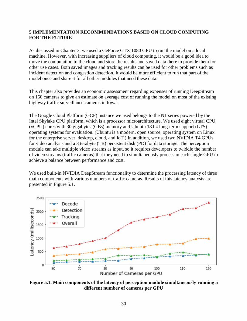
5 IMPLEMENTATION RECOMMENDATIONS BASED ON CLOUD COMPUTING
FOR THE FUTURE
As discussed in Chapter 3, we used a GeForce GTX 1080 GPU to run the model on a local
machine. However, with increasing suppliers of cloud computing, it would be a good idea to
move the computation to the cloud and store the results and saved data there to provide them for
other use cases. Both saved images and tracking results can be used for other problems such as
incident detection and congestion detection. It would be more efficient to run that part of the
model once and share it for all other modules that need these data.
This chapter also provides an economic assessment regarding expenses of running DeepStream
on 160 cameras to give an estimate on average cost of running the model on most of the existing
highway traffic surveillance cameras in Iowa.
The Google Cloud Platform (GCP) instance we used belongs to the N1 series powered by the
Intel Skylake CPU platform, which is a processor microarchitecture. We used eight virtual CPU
(vCPU) cores with 30 gigabytes (GBs) memory and Ubuntu 18.04 long-term support (LTS)
operating systems for evaluation. (Ubuntu is a modern, open source, operating system on Linux
for the enterprise server, desktop, cloud, and IoT.) In addition, we used two NVIDIA T4 GPUs
for video analysis and a 3 terabyte (TB) persistent disk (PD) for data storage. The perception
module can take multiple video streams as input, so it requires developers to twiddle the number
of video streams (traffic cameras) that they need to simultaneously process in each single GPU to
achieve a balance between performance and cost.
We used built-in NVIDIA DeepStream functionality to determine the processing latency of three
main components with various numbers of traffic cameras. Results of this latency analysis are
presented in Figure 5.1.
Figure 5.1. Main components of the latency of perception module simultaneously running a
different number of cameras per GPU

31
For the purpose of processing data in near real-time, we distributed 80 cameras to each T4 GPU
so that the overall processing latency caused by the perception module was less than 1 second.
Thus, the total of 160 cameras was split into two T4 GPUs where the average GPU memory
usage was around 65%. In other words, the number of cameras could be decided by a traffic
agency based on their tolerance of processing delay without necessarily exceeding the total GPU
memory.
In the perception module, six consecutive frames were skipped at the model inference stage for
computational efficiency. The coexisting CUDA 10.2 and CUDA 10.1 GPU drivers version
418+ and TensorRT 7.0 were used to improve the performance of the NVIDIA T4 GPU
according to the T4 workaround specification (NVIDIA 2020a).Kafka 2.4, Spark 2.4.5, and
Elasticsearch/Kibana 7.5.2 were used in the analysis module. (Kibana is an open source data
visualization dashboard for Elasticsearch, and Elasticsearch is a search engine based on the
Lucene library.) In Table 5.1, we summarize the computational resource usage for running our
framework on the GCP.
Table 5.1. Summary of computational resource usage on the GCP
Container CPU Memory GPU memory (Per GPU) GPU Util (Per GPU)
Perception0 22.3% 6.9% 65.5% 71.0%
Perception1 21.6% 6.5% 64.1% 69.0%
Kakfa 3.8% 2.2% 0% 0%
Spark 30.6% 29.8% 0% 0%
Elasticsearch 10.3% 3.3% 0% 0%
Kibana 0.18% 0.4% 0% 0%
To measure the operating costs in detail, we implemented the proposed framework using the
GCP for 5 days. The GCP provides a sustained use discount cost based on monthly usage level.
In Figure 5.2, we show the average daily cost with (left) and without (right) the sustained use
discount.
Figure 5.2. Daily operating costs for 160 cameras with sustained use discount (left) and
without sustained use discount (right)

32
The daily operating cost for 160 cameras was $21.59 with the sustained use discount (assuming
such a traffic video analysis framework would be operating for the long term). The GPUs and
vCPUs are the two major costs, which made up 46.4% and 19.7%, respectively, of the total cost,
while the persistent storage, network, and random access memory (RAM) together made up
33.9% of the total cost. Thus, the daily cost of the proposed framework for each camera was
$0.135, leading to the yearly cost per camera of $49.30.
Iowa has 390 operating traffic surveillance cameras on the road network. Thus, turning all of
these surveillance cameras into connected smart sensors would cost $1,601.40 per month using
this cloud-enabled system, with the benefit of eliminating additional infrastructure costs.

33
REFERENCES
Babic, S., M. I. Valic, S. Golob, and T. Tekavec. 2010. Proposal for a New Method for Wrong
Way Detection. https://sipronika.si/.
Baratian-Ghorghi, F., H. Zhou, and J. Shaw. 2014. Overview of Wrong-Way Driving Fatal
Crashes in the United States. ITE Journal, Vol. 84, No. 8, pp. 41–47.
Bewley, A., Z. Ge, L. Ott, F. Ramos, and B. Upcroft. 2016. Simple Online and Realtime
Tracking. 2016 IEEE International Conference on Image Processing (ICIP), pp. 3464–
3468.
Cooner, S. A., A. S. Cothron, and S. E. Ranft. 2004. Countermeasures for Wrong-Way
Movement on Freeways: Overview of Project Activities and Findings. Texas
Transportation Institute, Texas A&M University System, College Station, TX.
GStreamer. 2019. Gstreamer Open Source Multimedia Framework.
Gunay, E. E., G. E. O. Kremer, and A. Zarindast. 2020. A Multi-Objective Robust Possibilistic
Programming Approach to Sustainable Public Transportation Network Design. Fuzzy
Sets and Systems.
Ha, S. V.-U., L. H. Pham, H. M. Tran, and P. H. Thanh. 2014. Improved Optical Flow
Estimation in Wrong Way Vehicle Detection. Journal of Information Assurance &
Security, Vol. 9, No. 7.
Haendeler, S., A. Lewandowski, and C. Wietfeld. 2014. Passive Detection of Wrong Way
Drivers on Motorways Based on Low Power Wireless Communications. 2014 IEEE 79th
Vehicular Technology Conference (VTC Spring), pp. 1–5.
Haghighat, A. K., V. Ravichandra-Mouli, P. Chakraborty, Y. Esfandiari, S. Arabi, and A.
Sharma. 2020. Applications of Deep Learning in Intelligent Transportation Systems.
Journal of Big Data Analytics in Transportation, Vol. 2, No. 2, pp. 115–145.
He, K., X. Zhang, S. Ren, and J. Sun. 2016. Deep Residual Learning for Image Recognition.
2016 IEEE Conference on Computer Vision and Pattern Recognition (CVPR), pp. 770–
778.
Huang, T. 2020. Designing the Next Generation Intelligent Transportation Sensor System Using
Big Data Driven Machine Learning Techniques. PhD dissertation. Iowa State University,
Ames, IA.
Jain, A. M. and N. Tiwari. 2015. Airborne Vehicle Detection with Wrong-Way Drivers Based on
Optical Flow. International Conference on Innovations in Information, Embedded and
Communication Systems (ICIIECS), pp. 1–4.
Kaminski Leduc, J. L. 2008. Wrong Way Driving Countermeasures. Office of Legislative
Research (OLR) Research Report. Connecticut General Assembly, Hartford, CT.
Mampilayil, H. R. and K. Rahamathullah. 2019. Deep Learning Based Detection of One Way
Traffic Rule Violation of Three Wheeler Vehicles. 2019 International Conference on
Intelligent Computing and Control Systems (ICCS), May 15–17, Madurai, India, pp.
1453–1457.
MH Corbin. 2020. The Right Solution for Wrong-Way Driving.
https://mhcorbin.com/Solutions/Wrong-Way-Detection.
Morena, D. A. and T. J. Leix. 2012. Where These Drivers Went Wrong. Public Roads, Vol. 75,
No. 6.
Moler, S. 2002. Stop. You’re Going the Wrong Way! Public Roads, Vol. 66, No. 2.

34
Monteiro, G., M. Ribeiro, J. Marcos, and J. Batista. 2007. Wrong Way Drivers Detection Based
on Optical Flow. 2007 IEEE International Conference on Image Processing, Vol. 5, pp.
141–144.
NVIDIA Corporation. 2020a. NVIDIA DeepStream SDK.
https://developer.nvidia.com/deepstream-sdk.
NVIDIA Corporation. 2020b. NVIDIA Transfer Learning Toolkit.
https://developer.nvidia.com/transfer-learning-toolkit.
NVIDIA Corporation. 2020c. Smart Parking Detection.
https://ngc.nvidia.com/catalog/containers/nvidia:deepstream_360d.
Pour-Rouholamin, M., H. Zhou, J. Shaw, and P. Tobias. 2015. Current Practices of Safety
Countermeasures for Wrong-Way Driving Crashes. 94th Annual Meeting of the
Transportation Research Board, January 11–15, Washington, DC.
Rajabalizadeh, A., J. N. Nia, N. Safaei, M. Talafidaryani, R. Bijari, A.Zarindast, F. Fotouhi, M.
Salehi, and M. Moqri. 2020. Exploratory Analysis of Electronic Intensive Care Unit
(eICU). medRxiv.
Redmon, J. and A. Farhadi. 2018. YOLOv3: An Incremental Improvement. arXiv. Cornell
University, Ithaca, NY.
Rosebrock, A. 2018. OpenCV OCR and Text Recognition with Tesseract.
https://www.pyimagesearch.com/2018/09/17/opencv-ocr-and-text-recognition-with-
tesseract/.
Sentas, A., S. Kul, and A. Sayar. 2019. Real-Time Traffic Rules Infringing Determination Over
the Video Stream: Wrong Way and Clearway Violation Detection. 2019 International
Artificial Intelligence and Data Processing (IDAP) Symposium, Malatya, Turkey, pp. 1–
4.
Simpson, S. A. 2013. Wrong-Way Vehicle Detection: Proof of Concept. Arizona. Department of
Transportation, Phoenix, AZ.
Sreelatha, R., R. Roopalakshmi, and K. A. Bharadwaj. 2020. An Enhanced Traffic Abnormality
Detection System for Vehicle Characteristics Tracking Using Radar Signals. 2020 2nd
International Conference on Innovative Mechanisms for Industry Applications (ICIMIA),
pp. 1–4.
Steux, B, C. Laurgeau, L. Salesse, and D. Wautier. 2002. Fade: A Vehicle Detection and
Tracking System Featuring Monocular Color Vision and Radar Data Fusion. Intelligent
Vehicle Symposium, Vol. 2, pp. 632–639.
Zarindast, A., E. E. Gunay, K. Park, and G. E. Okudan Kremer. 2018. Determination of Bus
Station Locations under Emission and Social Cost Constraints. Proceedings of the 2018
IISE Annual Conference and Expo. May 19–22, Orlando, FL.
Zarindast, A. 2019. A Data Driven Method for Congestion Mining Using Big Data Analytics.
MS thesis. Iowa State University, Ames, IA.
Zhou, H., J. Zhao, R. Fries, M. R. Gahrooei, L. Wang, B. Vaughn, K. Bahaaldin, and B.
Ayyalasomayajula. 2012. Investigation of Contributing Factors Regarding Wrong-Way
Driving on Freeways. Illinois Center for Transportation, University of Illinois at Urbana-
Champaign, Urbana, IL.


THE INSTITUTE FOR TRANSPORTATION IS THE FOCAL POINT FOR TRANSPORTATION AT IOWA STATE UNIVERSITY.
InTrans centers and programs perform transportation research and provide technology transfer services for government agencies and private companies;
InTrans contributes to Iowa State University and the College of Engineering’s educational programs for transportation students and provides K–12 outreach; and
InTrans conducts local, regional, and national transportation services and continuing education programs.
Visit InTrans.iastate.edu for color pdfs of this and other research reports.