AUTOMATIC RECONSTRUCED ROOF SHAPES FOR LIDAR STRIP ADJUSTMENT AND QUALITY CONTROL

M. Rentsch *, P. Krzystek

University of Applied Sciences Muenchen, Department of Geographic Information Sciences, 80333 Munich, Germany

- (rentsch, krzystek)@hm.edu

Commission III, WG III/2

KEY WORDS: LIDAR, Reconstruction, Adjustment, Building, Point Cloud, Quality ABSTRACT: In the recent years, the performance of LiDAR systems was improved by acquisition of the terrain surface with steadily increasing point densities. However, the main error sources affecting the quality of LiDAR derived secondary products like DTMs and DSMs are resulting from systematic residual errors coming from insufficient calibration and strip adjustment, and from deficiencies in classification and filtering of the laser points. The systematic errors are recognized as discrepancies of the laser point clouds in overlapping areas of neighboring LiDAR strips. In this work, the main focus is on a new 3D measurement technique based on intersecting roof ridge lines and roof planes which are automatically reconstructed from the laser point clouds. The coordinate differences between conjugate intersection points are incorporated in an adjustment process to resolve for the residual errors of each LiDAR strip separately. The new 3D reconstruction method is applied on two different datasets, consisting of last pulse and full waveform data, and also taking advantage of full waveform measurements like intensity and pulse width which are decomposed from the waveforms. In general, the results show that significant discrepancies mainly in position still exist. After the strip adjustment and correction, the relative horizontal displacements between adjacent strips are improved significantly by more than 70%. The investigations also show that the higher laser point density of full waveform LiDAR data (3-5 points/m2) leads to better results after the adjustment with respect to the last pulse dataset (density 1-2 points/m2).

* Corresponding author.

1. INTRODUCTION

Geospatial databases are essential for describing the Earth’s surface with the requirement of high quality and being up-to-date. LiDAR has been established as technology for fast and high-resolution acquisition of the terrain surface. Major secondary products of LiDAR data are DTMs and DSMs for various applications in geosciences. Due to the rapidly growing amount of LiDAR data in the recent years, the users were increasingly faced with the cost-intensive collection, continuation and quality assessment of geospatial databases. The dominant sources affecting the quality of LiDAR derived products are residual errors coming from insufficient calibration and strip adjustment, and errors in data classification and filtering. In most cases, LiDAR data acquisition is conducted by private companies who also perform the pre-processing, the classification and the quality control. Nevertheless, subsequent quality investigations still exhibit horizontal and vertical offsets which are clearly visible at distinct objects (e.g. roof profiles) in overlapping areas of adjacent tracks. In the literature, various methods have been proposed for the adequate measurement of horizontal and vertical offsets. Burman (2002) derives the height discrepancy for a laser point of a strip by relating the position to the TIN surface of an adjacent strip. Maas (2002) is generating local TINs for small areas in overlapping strips and derives 3D offsets through a least squares matching between the selected subsets. The focus in Filin and Vosselman (2004) and Pfeifer et al. (2005) is on the extraction of suitable planar segments (natural or man-made)

for the determination of corresponding tie and control elements in different LiDAR strips. Pfeifer et al. (2005) select surface elements and determine strips offsets by comparing the barycenters of the selected surfaces. In the recent years, the emphasis was also on the extraction of building roof shapes as tie elements. The fully 3D adjustment approach of Kager (2004) incorporates three (neighboured) homologues planes equivalent to a fictitious tying point. Pothou et al. (2008) conduct the estimation of boresight misalignment parameters by comparing LiDAR derived roof surfaces with photogrammetrically reconstructed reference surfaces. Ahokas et al. (2004) are using ridge lines for a comparison study with repeated LiDAR observations. Habib et al. (2008) are computing corresponding linear features from intersections of roof planes in overlapping LiDAR strips. The linear features are represented by its end points and their coordinate discrepancies between different strips serve as input for a strip adjustment and quality control. Vosselman (2008) presents a largely automatic procedure for assessing the planimetric accuracy of three LiDAR surveys in the Netherlands. Relative horizontal shifts between overlapping areas of adjacent strips are measured by detection and comparison of reconstructed roof ridge lines derived from the LiDAR data. The main focus of the presented work is on the development of a new method for the precise 3D measurement of remaining horizontal and vertical offsets between overlapping areas of adjacent LiDAR strips. For this purpose, appropriate roof shapes with crossing ridge lines are reconstructed from the laser point clouds. Then, 2D and 3D points are derived by

In: Bretar F, Pierrot-Deseilligny M, Vosselman G (Eds) Laser scanning 2009, IAPRS, Vol. XXXVIII, Part 3/W8 – Paris, France, September 1-2, 2009Contents Keyword index Author index

117

intersecting the roof planes and ridge lines for each strip separately. The approach is basically suitable for full waveform data comprising the pulse energy (viz. the intensity) and the pulse width as additional laser point attributes. The strip-to-strip coordinate differences of the 2D and 3D intersection points represent the displacements which are mainly caused by residual systematic errors concerning the laser range measurement, GPS position, IMU attitudes and the alignment of the LiDAR system components. The relation of measured horizontal and vertical offsets and residual errors is modeled by a simplified 3D transformation. By introducing the offset measurements as observations, the residual errors for shifts and rotations are resolved by means of an adjustment approach and finally, the resulting corrections are applied to the laser points. The paper is organized as follows. Section 2 highlights the strip adjustment model and the reconstruction of roof shapes. Section 4 addresses the results we obtained with two datasets com-prising last pulse and full waveform data. Finally, the results are discussed in Section 5 with conclusions given in Section 6.

2. METHODS

2.1 Concept

Due to the strip-wise acquisition of LiDAR surveys, the systematic errors are supposed to affect the coordinate offsets for each strip separately (Figure 1). For simplification, some assumptions are defined for the mathematical model of our approach (Equation 1).

Figure 1. Sample configuration of LiDAR strips with control

(green) and tie elements (orange). As example, relative horizontal offsets ∆X’ and ∆Y’ between overlapping strips are

measured for a tie element (violet)

⎟⎟⎟

⎠

⎞

⎜⎜⎜

⎝

⎛+

⎟⎟⎟

⎠

⎞

⎜⎜⎜

⎝

⎛

−−−

⋅⎟⎟⎟

⎠

⎞

⎜⎜⎜

⎝

⎛=

⎟⎟⎟

⎠

⎞

⎜⎜⎜

⎝

⎛

0i

0i

0i

siik

siik

siik

i

ii

i

'ik

'ik

'ik

ZYX

zzyyxx

1∆r0∆r-1∆h0∆h-1

ZYX

(1)

where X'ik , Y'ik , Z'ik Coordinates of laser point k of corrected strip i ∆ri , ∆hi Rotation angles for roll and heading of strip i xik , yik , zik Coord. of laser point k of uncorrected strip i X0i , Y0i , Z0i Shifts of uncorrected strip i xi

s , yis , zi

s Centroid of uncorrected strip i

First, time dependent portions are not considered. The rotation angles (roll and heading) are assumed as small values and no rotation angle along the y-axis of a strip i is applied. This means that we do not compensate for a pitch angle error which causes essentially a horizontal shift in the laser points. The error model resp. the observation equations are established in a local strip coordinate system in which the strip centroids represent the origin and the local x-axis is approximately aligned to the flight direction prior to the strip adjustment procedure (Vosselman and Maas, 2001). The unknown parameters of each strip i are found in a combined adjustment using control and tie elements. Control and tie elements are usually horizontal, vertical or 3D elements measured by an appropriate measurement technique. 2.2 Automatic reconstruction roof shapes

The new method has been developed to derive 2D as well as 3D points from the intersection of modeled roof ridge lines coming from different LiDAR strips. The main processing steps can be divided as follows: (1) Selection of buildings with appropriate roof surfaces, e.g. L-shaped or T-shaped. (2) Separation of roof points from bare Earth points. Herein, the separation is supported by predetermined building outlines or, if not available, by dividing the points according to their pre-classified point class and height values. (3) Computation of geometric and physical laser point features. At each laser point location, a local fitting RANSAC plane is computed from the surrounding points (Figure 2). According to the given point density, an appropriate search radius is determined to ensure that a predefined number of points (e.g. 30) is included. Laser points for which the height variations with respect to the local plane exceed a defined threshold (this appears for example for points on a roof ridge) are rejected. Afterwards, for each selected laser point, a list of features is determined: The xyz-components of the plane normal vector nx, ny and nz, the orientation of the roof plane po=arctan(nx/ny) (Fig. 3.1), the laser intensity and the pulse width (Fig. 3.2 and 3.3). Note that the features intensity and pulse width are optional and are dedicated to full waveform LiDAR systems. They can be calculated via waveform decomposition (Reitberger et al., 2008). Here, the intensity is understood as the pulse energy that can be calculated from the amplitude and the pulse width of a single return. (4) Segmentation of roof planes by means of clustering using the derived features. A preliminary clustering of laser points is performed by the k-means algorithm and a given number of clusters. For each of the found clusters, common features as described before are derived and assigned. Tiny clusters with a very small number of points (e.g. 5) are apparently discarded (Fig. 3.4). Then, the clusters undergo a hierarchical clustering which leads to a merging of clusters with nearly coinciding features and resulting to clearly separated roof planes. (5) Finally, an adjusting plane is computed including all laser points from each merged cluster. Laser points on small features like chimneys or dormers are detected by means of their distance to the adjusting plane and are filtered out. (6) Evaluation of roof ridge lines by means of plane intersections. The appropriate roof planes which are used for plane intersection are selected according to their features (e.g. opposite orientation) and are intersected, leading to a pair of ridge lines in the normal case. (7) Derivation of 2D points from line intersections and 3D points from plane-line intersection. Because the extracted ridge lines are representing skewed straight lines in space, a 3D intersection between them cannot be carried out. However, a 2D intersection is always feasible meaning that the X- and Y-coordinates of a ridge line intersection are always ascertained. Fully 3D coordinates can be

In: Bretar F, Pierrot-Deseilligny M, Vosselman G (Eds) Laser scanning 2009, IAPRS, Vol. XXXVIII, Part 3/W8 – Paris, France, September 1-2, 2009Contents Keyword index Author index

118

achieved by intersecting the lower of the two ridge lines with the opposite roof planes, resulting in two intersection points (Figure 4). (8) Finally, the coordinate differences of conjugate 2D and 3D intersection points in overlapping strip areas can be calculated, revealing the spatial offsets caused by remaining shifts and rotations (Figure 5).

2.3

Figure 2. Construction of local fitting RANSAC plane at each

laser point location

Fig. 3.1. Plane orientation po Fig. 3.2. Laser intensity

Fig. 3.3. Pulse width Fig. 3.4. Preliminary plane clustering (with chimneys and dormers)

Figure 4. Calculation of 2D and 3D intersection points

Figure 5. Determination of 2D and 3D offsets

Strip Adjustment

For this purpose, two basic types of observation equations are established. Equation 2 stands for an absolute measurement for a control element, Equation 3 for a relative measurement between overlapping strips and are given as follows

⎟⎟⎟

⎠

⎞

⎜⎜⎜

⎝

⎛+

⎟⎟⎟

⎠

⎞

⎜⎜⎜

⎝

⎛

−−−

⋅⎟⎟⎟

⎠

⎞

⎜⎜⎜

⎝

⎛=

⎟⎟⎟

⎠

⎞

⎜⎜⎜

⎝

⎛+

⎟⎟⎟

⎠

⎞

⎜⎜⎜

⎝

⎛

0i

0i

0i

siik

siik

siik

i

ii

i

Z

Y

X

'ik

'ik

'ik

ZYX

zzyyxx

1∆r0∆r-1∆h0∆h-1

vvv

ZYX (2)

−⎟⎟⎟

⎠

⎞

⎜⎜⎜

⎝

⎛

−−−

⋅⎟⎟⎟

⎠

⎞

⎜⎜⎜

⎝

⎛=

⎟⎟⎟

⎠

⎞

⎜⎜⎜

⎝

⎛+⎟⎟⎟

⎠

⎞

⎜⎜⎜

⎝

⎛

siik

siik

siik

i

ii

i

∆Z

∆Y

∆X

'ijk

'ijk

'ijk

zzyyxx

1∆r0∆r-1∆h0∆h-1

vvv

∆Z∆Y∆X

⎟⎟⎟

⎠

⎞

⎜⎜⎜

⎝

⎛

−−−

+⎟⎟⎟

⎠

⎞

⎜⎜⎜

⎝

⎛

−−−

⋅⎟⎟⎟

⎠

⎞

⎜⎜⎜

⎝

⎛

0j0i

0j0i

0j0i

sjjk

sjjk

sjjk

j

jj

j

ZZYYXX

zzyyxx

1∆r0∆r-1∆h0∆h-1 (3)

where X'ik , Y'ik , Z'ik represent the measurements on a control element k in the strip i, and ∆X'ijk , ∆Y'ijk , ∆Z'ijk are the offset measurements between strip i and j on a tie element k. The terms vX, vY, vZ stand for the residuals of the measurements on a control element, and v∆X, v∆Y, v∆Z for the residuals of the measurements on a tie element. The unknown shifts of strip i are given by X0i, Y0i, Z0i, and the unknown rotation angles (compensating IMU rotations roll and heading) for the strip i by ∆ri and ∆hi. The coordinates xi

S, yiS,zi

S of the strip centroids are calculated from laser points of the uncorrected strip. For the strip adjustment, six different observation types are introduced; type 1-3 belonging to Equation 2, type 4-6 to Equation 3. The measurements of vertical discrepancies (observation types 1 and 4) are not described in this context, for more details see Rentsch and Krzystek (2009). For the stochastic model, each of the observation types can be assigned with individual a-priori standard deviations reflecting their varying accuracy levels.

Obs. Type Description

1 Absolute vertical measurement with respect to a height control element (e.g. soccer field)

2 Absolute horizontal measurements with respect to a control element

3 Absolute 3D measurements with respect to a control element

4 Relative vertical offset measurement between adjacent strips for a tie element

5 Relative horizontal offset measurement between adjacent strips for a tie element

6 Relative 3D offset measurement between adjacent strips for a tie element

Table 1. Observation types used within the strip adjustment

3. MATERIAL

The algorithms were evaluated with two different datasets. The first project ‘Kempten’ is located in Southern Bavaria and was surveyed in May 2006 (Figure 6). The entire project area was flown strip wise with a direction deviating about 30 degrees against east-west. With a predefined flight altitude of 1000 m and a scan angle of 22 degrees, this led to strip width of around 800 m. 45 % were chosen as across-track overlap resulting in approximately 300 m wide common areas of adjacent strips.

In: Bretar F, Pierrot-Deseilligny M, Vosselman G (Eds) Laser scanning 2009, IAPRS, Vol. XXXVIII, Part 3/W8 – Paris, France, September 1-2, 2009Contents Keyword index Author index

119

The data were recorded with a first/last pulse scanner (Optech ALTM-3100). The mean point density is about 1-2 points/m2. The size of the investigation area is 13.2 x 7.2 km including eight parallel LiDAR strips.

Figure 6. Dataset ‘Kempten’ (Blue squares = vertical offsets; Red squares = 2D/3D offsets; Red triangles = control elements;

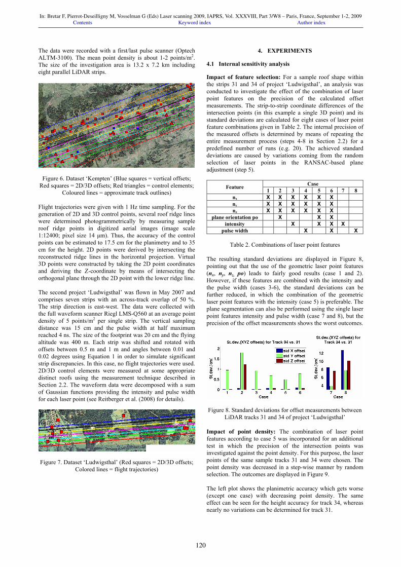
Coloured lines = approximate track outlines) Flight trajectories were given with 1 Hz time sampling. For the generation of 2D and 3D control points, several roof ridge lines were determined photogrammetrically by measuring sample roof ridge points in digitized aerial images (image scale 1:12400; pixel size 14 µm). Thus, the accuracy of the control points can be estimated to 17.5 cm for the planimetry and to 35 cm for the height. 2D points were derived by intersecting the reconstructed ridge lines in the horizontal projection. Virtual 3D points were constructed by taking the 2D point coordinates and deriving the Z-coordinate by means of intersecting the orthogonal plane through the 2D point with the lower ridge line. The second project ‘Ludwigsthal’ was flown in May 2007 and comprises seven strips with an across-track overlap of 50 %. The strip direction is east-west. The data were collected with the full waveform scanner Riegl LMS-Q560 at an average point density of 5 points/m2 per single strip. The vertical sampling distance was 15 cm and the pulse width at half maximum reached 4 ns. The size of the footprint was 20 cm and the flying altitude was 400 m. Each strip was shifted and rotated with offsets between 0.5 m and 1 m and angles between 0.01 and 0.02 degrees using Equation 1 in order to simulate significant strip discrepancies. In this case, no flight trajectories were used. 2D/3D control elements were measured at some appropriate distinct roofs using the measurement technique described in Section 2.2. The waveform data were decomposed with a sum of Gaussian functions providing the intensity and pulse width for each laser point (see Reitberger et al. (2008) for details).

Figure 7. Dataset ‘Ludwigsthal’ (Red squares = 2D/3D offsets;

Colored lines = flight trajectories)

4. EXPERIMENTS

4.1 Internal sensitivity analysis

Impact of feature selection: For a sample roof shape within the strips 31 and 34 of project ‘Ludwigsthal’, an analysis was conducted to investigate the effect of the combination of laser point features on the precision of the calculated offset measurements. The strip-to-strip coordinate differences of the intersection points (in this example a single 3D point) and its standard deviations are calculated for eight cases of laser point feature combinations given in Table 2. The internal precision of the measured offsets is determined by means of repeating the entire measurement process (steps 4-8 in Section 2.2) for a predefined number of runs (e.g. 20). The achieved standard deviations are caused by variations coming from the random selection of laser points in the RANSAC-based plane adjustment (step 5).

Case Feature 1 2 3 4 5 6 7 8 nx X X X X X X ny X X X X X X nz X X X X X X

plane orientation po X X X intensity X X X X

pulse width X X X

Table 2. Combinations of laser point features

The resulting standard deviations are displayed in Figure 8, pointing out that the use of the geometric laser point features (nx, ny, nz, po) leads to fairly good results (case 1 and 2). However, if these features are combined with the intensity and the pulse width (cases 3-6), the standard deviations can be further reduced, in which the combination of the geometric laser point features with the intensity (case 5) is preferable. The plane segmentation can also be performed using the single laser point features intensity and pulse width (case 7 and 8), but the precision of the offset measurements shows the worst outcomes.

Figure 8. Standard deviations for offset measurements between

LiDAR tracks 31 and 34 of project ‘Ludwigsthal’

Impact of point density: The combination of laser point features according to case 5 was incorporated for an additional test in which the precision of the intersection points was investigated against the point density. For this purpose, the laser points of the same sample tracks 31 and 34 were chosen. The point density was decreased in a step-wise manner by random selection. The outcomes are displayed in Figure 9. The left plot shows the planimetric accuracy which gets worse (except one case) with decreasing point density. The same effect can be seen for the height accuracy for track 34, whereas nearly no variations can be determined for track 31.

In: Bretar F, Pierrot-Deseilligny M, Vosselman G (Eds) Laser scanning 2009, IAPRS, Vol. XXXVIII, Part 3/W8 – Paris, France, September 1-2, 2009Contents Keyword index Author index

120

Figure 9. Intersection accuracy (left=planimetric, right=height)

vs. point density for tracks 31 and 34 4.2 Adjustment results

The adjustment process was performed according to the mathematical model given by Equations 2 and 3 with the number of observations shown in Tables 3 and 4. The redundancy was 330 for dataset ‘Kempten’ and 683 for dataset ‘Ludwigsthal’. As mentioned in Section 2.3, the different observation types had to be handled individually in terms of their varying standard deviations. As consequence, a variance component analysis (VCA) was conducted to achieve suitable a-priori standard deviations to be incorporated into the stochastic model (Tables 3 and 4). The comparison of the standard deviations before (sigma a-priori) and after the strip adjustment (sigma a-posteriori) for the individual observation types reveal a high consistency, confirming that the stochastic model is appropriate to account for individual precision levels.

Obs. Type

sigma naught (a-priori) [cm]

sigma naught (a-posteriori) [cm]

#Obs.

1 9.5 9.4 2 2 13.0 12.7 4 3 19.0 (planimetry),

12.0 (height) 18.6 (planimetry), 11.7

(height) 42

4 8.5 8.4 5 5 8.5 7.2 68 6 8.5 (planimetry),

7.0 (height) 8.3 (planimetry),

6.6 (height) 249

Table 3. Standard deviations before and after strip adjustment

for each observation type separately (project ‘Kempten’)

Obs. Type

sigma naught (a-priori) [cm]

sigma naught (a-posteriori) [cm]

#Obs.

5 4.5 4.5 184 6 5.4 (planimetry),

3.6 (height) 4.8 (planimetry),

3.6 (height) 498

Table 4. Standard deviations before and after strip adjustment for each observation type separately (project ‘Ludwigsthal’)

4.3 Strip correction and validation

The corrections for the project ‘Kempten’ were applied for each LiDAR strip using the flight trajectories consisting of the 1-s GPS positions, the date and time and the GDOP (global dilution of precision). For each laser point location, the measurement constellation was reconstructed by calculating the orthogonal plane of the trajectory including the uncorrected laser point. Then, the derived shifts and rotations resulting from the adjustment were applied to the points of each LiDAR strip separately. In the case of project ‘Ludwigsthal’, the correction of the laser points was calculated just using Equation 1. Finally, the 3D measurement technique was carried out for the corrected

laser points revealing that the relative displacements between adjacent strips could be significantly reduced (Tables 5 and 6).

r.m.s. planimetry [cm] r.m.s. height [cm] before strip adjustment 35.6 9.5

after strip adjustment 10.2 6.6

Table 5. Relative displacements of 50 virtual check elements

before and after strip adjustment (project ‘Kempten’)

r.m.s. planimetry [cm] r.m.s. height [cm] before strip adjustment 58.5 49.9

after strip adjustment 5.9 5.2

Table 6. Relative displacements of 66 virtual check elements

before and after strip adjustment (project ‘Ludwigsthal’)

5. DISCUSSION

The main focus of the present work is on a new and precise 3D measurement technique for the determination of horizontal and vertical offsets between overlapping regions of adjacent LiDAR strips. The discrepancies can be measured using the intersection points of reconstructed roof ridge lines and roof planes. The high accuracy level of the proposed method is revealed in Tables 3 and 4 showing estimated standard deviations after the strip adjustment of about 8 cm (planimetry) and 7 cm (height) for the block ‘Kempten’ resp. 5 cm (planimetry) and 4 cm (height) for the block ‘Ludwigsthal’. However, the control points in Table 3 show standard deviations that are roughly worse by a factor 2. This can be mostly attributed to unresolved systematic errors in the photogrammetric stereo models which reduce the absolute measuring accuracy. Interestingly, the estimated accuracy is for both blocks worse than the precision delivered by the new measurement technique (see Section 4.1 and Figure 8). This disagreement can be explained on the one hand by a non-perfect tie element configuration causing a weak adjustment result. Also, non-linear strip deformations caused by e.g. non-adequate IMU measurements during jerky platform movements or uncalibrated non-linear scan angle errors might not sufficiently be modelled in case of the block ‘Kempten’ by the mathematical model (Equation 1). Moreover, another reason might be that in some cases the roof structures are not correctly represented by the intersecting planes, thus causing a larger intersection error due to the inadequate geometric model. Similar effects could be observed by Vosselman and Maas (2001) and Maas (2002) who report on a precision of the applied TIN least-squares matching of 10 cm and estimated standard deviations after the strip adjustment (Block Eelde) of 25 cm in planimetry and 8.5 cm in height. The measured offsets are incorporated in a strip adjustment approach to resolve for remaining shifts and rotations between LiDAR strips. Vertical shifts of a few centimeters and horizontal shifts with a magnitude higher are resolvable for the already pre-adjusted LiDAR strips in case of project ‘Kempten’ (see Table 5). Filin and Vosselman (2004) have detected comparable horizontal offsets by analysing 10 parallel and 10 crossing strips. The resolved rotations are marginal with respect

In: Bretar F, Pierrot-Deseilligny M, Vosselman G (Eds) Laser scanning 2009, IAPRS, Vol. XXXVIII, Part 3/W8 – Paris, France, September 1-2, 2009Contents Keyword index Author index

121

to the derived shifts, thus a simple horizontal shift of the laser strips is sufficient for an significant improvement (see also Vosselman (2008)). Correcting the strips of the block ‘Kempten’ with the adjusted strip parameters improves the horizontal discrepancies between the LiDAR strips by 70%. Nearly no improvement is achieved for the vertical discrepancies which are below 10 cm anyway before the adjustment. The results are comparable to the findings from Vosselman and Maas (2001), in which the degree of improvement was around 40% for the horizontal discrepancies. The remaining relative r.m.s. displacements after the strip adjustment of the project ‘Ludwigsthal’ mainly reveal the total accuracy the 3D measuring technique can provide for the selected roof shapes in this project area. All in all, the r.m.s. displacements after the strip adjustment in Tables 5 and 6 match quite well with the estimated accuracy for both blocks after the adjustment (Tables 3 and 4), showing the appropriate correction of the laser points with the adjusted strip parameters. The r.m.s. displacements after the strip adjustment clearly reveal that the precision of the full waveform dataset ‘Ludwigsthal’ is better roughly by a factor 2. This can be explained by the different length of the LiDAR strips, in which the larger LiDAR strips of the last pulse dataset ‘Kempten’ (around 13 km) are possibly more affected by non-linear strip deformations than the LiDAR strips of dataset ‘Ludwigsthal’ with a mean strip length of around 7 km. Moreover, the precision of the 3D measurement technique is dependent on the laser point density which was demonstrated for a sample roof in two strips. This leads to the assumption that the performance of the proposed method will benefit from a high point density. In addition, with increasing point density, smaller roof surfaces can be incorporated as adequate objects into the proposed measurement approach to optimize the configuration of the tie points. Furthermore, the precision of the 3D measurement technique is minimized if all the geometric features (nx, ny, nz and po) are combined with the intensity and pulse width. Thus, all in all, the comparison between the two blocks show that the usage of highly dense full waveform LiDAR points plus the intensity and pulse width as additional point attributes leads to a better strip adjustment accuracy.

6. CONCLUSIONS

The experiments of this study point out that significant discrepancies still exist between individual LiDAR strips. These offsets can be detected by visual inspections, a common but cost-intensive and time-consuming practice often performed by end-users like survey administrations. With a new 3D measurement technique based on reconstructed roof shapes and roof ridge lines, remaining horizontal and vertical discrepancies between LiDAR strips now can be precisely detected, thus serving as a helpful tool for a comprehensive quality control. In addition, a subsequent strip adjustment can resolve systematic errors that are the reasons for the detected shifts. As expected, the method is dependent on the point density. Moreover, if full waveform data are available the intensity and the pulse width improve the precision of the method.

ACKNOWLEDGEMENTS

We thank Dr. Kistler and the Bavarian Office for Surveying and Geographic Information for their productive contributions and

for giving us the opportunity to use the dataset ‘Kempten’. This research has been funded by the German Department of Education and Research (BMBF) under the contract number 1714A06.

REFERENCES

Ahokas, E., H. Kaartinen, and J. Hyyppä, 2004. A quality assessment of repeated airborne laser scanner observations. Int. Arch. Photogramm. Remote Sens. Spat. Inf. Sci., 35 (B3), pp. 237-242.

Burman, H., 2002. Laser strip adjustment for data calibration and verification. Int. Arch. Photogramm. Remote Sens., 34 (part 3A), pp. 67-72.

Filin, S., and G. Vosselman, 2004. Adjustment of airborne laser altimetry strips. Int. Arch. Photogramm. Remote Sens. Spat. Inf. Sci., 35 (B3), pp. 285-289.

Habib, A.F., A.P. Kersting, Z. Ruifang, M. Al-Durgham, C. Kim, and D.C. Lee, 2008. LiDAR strip adjustment using conjugate linear features in overlapping strips. Int. Arch. Photogramm. Remote Sens. Spat. Inf. Sci., 37 (part B1), pp. 385-390.

Kager, H., 2004. Discrepancies between overlapping laser scanner strips – simultaneous fitting of aerial laser scanner strips. Int. Arch. Photogramm. Remote Sens. Spat. Inf. Sci., 35 (B1), pp. 555-560.

Maas, H.-G., 2002. Methods for measuring height and planimetry discrepancies in airborne laserscanner data. Photogramm. Eng. Rem. S. 68(9), pp. 933-940.

Pfeifer, N., S. Oude Elberink, and S. Filin, 2005. Automatic tie elements detection for laser scanner strip adjustment. Int. Arch. Photogramm. Remote Sens. Spat. Inf. Sci., 36 (3/W19), pp. 174-179.

Pothou, A., C. Toth, S. Karamitsos, and A. Georgopoulos, 2008. An approach to optimize reference ground control requirements for estimating LiDAR/IMU boresight misalignment. Int. Arch. Photogramm. Remote Sens. and Spat. Inf. Sci., 37 (part B1), pp. 301-307.

Reitberger, J., P. Krzystek, and U. Stilla, 2008. Analysis of full waveform LiDAR data for the classification of deciduous and coniferous trees. Int. J. Remote Sens. 29(5), pp. 1407-1431.

Rentsch, M., and P. Krzystek, 2009. Precise quality control of LiDAR strips. Proceedings ASPRS 2009 Annual Conference, 9-13 Mar 2009, Baltimore, MD, 11 p.

Vosselman, G., 2008. Analysis of planimetric accuracy of airborne laser scanning surveys. Int. Arch. Photogramm. Remote Sens. Spat. Inf. Sci., 37 (part B3a), pp. 99-104.

Vosselman, G., and H.-G. Maas, 2001. Adjustment and filtering of raw laser altimetry data, Proceedings OEEPE Workshop on Airborne Laserscanning and Interferometric SAR for Detailed Digital Elevation Models, Stockholm, Sweden, 01-03 March, OEEPE Publication No. 40, 62-72.

In: Bretar F, Pierrot-Deseilligny M, Vosselman G (Eds) Laser scanning 2009, IAPRS, Vol. XXXVIII, Part 3/W8 – Paris, France, September 1-2, 2009Contents Keyword index Author index

122