Automatic Photograph Enhancement -...
6
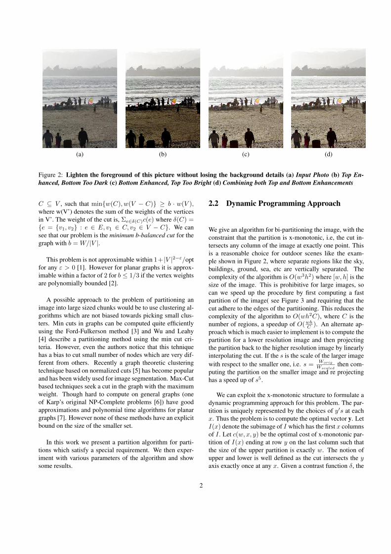
Automatic Photograph Enhancement Subhransu Maji [email protected] University of California at Berkeley Spring’07 Abstract We propose a method of image enhancement, based on a spatial domain technique called histogram equalization. Traditional histogram equalization is only useful for images with backgrounds and foregrounds that are both bright or both dark, whereas our method works for images with high dynamic range. The technique is to segment the image into large regions with high contrast separations which are then enhanced locally. The general problem of finding balanced cuts is NP-Hard and for the special case where the parti- tions have a special structure we give an polynomial time algorithm for finding good separations. Finally we demon- strate the algorithm on an example. 1 Introduction The aim of image enhancement is to improve the inter- pretability or perception of information in images for hu- man viewers, or to provide better’ input for other automated image processing techniques. The very nature of the prob- lem makes it ill posed, as there is no objective measure of quality. Spatial domain techniques enhance the image by finding a transform, T (f (x, y)) = g(x, y), in the image space. Examples include mean and median filters which are used for reducing noise in images. Frequency domain tech- niques work on the fourier transform of the image. Exam- ples include low pass filtering (analogous to blurring), Ho- momorphic filtering. Details of various techniques of image enhancement can be found in [10] and [11]. In this work we use a spatial domain filter called his- togram equalization. Histogram equalization is a method of contrast adjustment using the image’s histogram. It re- assigns intensities to the image so that the they are better distributed on a histogram thereby increasing its dynamic range. Excellent description of the theory of histogram equalization can be found in [10]. The method is useful in images with backgrounds and foregrounds that are both bright or both dark. In particular, the method can lead to bet- ter views of bone structure in x-ray images, and to better de- tail in photographs that are over or under-exposed. However Figure 1: Steps in the Enhancement Pipeline. for the images which already have a wide dynamic range, like the one shown Figure 2(a), histogram equalization does not work well (see Figure 5(c)). In this project we propose to enhance the image by breaking down an image into regions of similar intensities and apply local histogram equalization on each of the re- gions. For the histograms to be reliable each of the regions have to be large, and for histogram equalization to work well the regions should have high inter region contrast and low intra region contrast. The image enhancement pipeline (Figure 1) in the above formulation can be seen a combina- tion of two steps (1) Image Partitioning (2) Image Enhance- ment. In the sections that follow we describe the choices of algorithms for each of the steps, and present an approxima- tion scheme for (1), when the partition has a special struc- ture. 2 Image Partitioning Theoretical Abstraction: Given a target weight W and a planar graph G a with nodes representing the pixels, and edges denoting the similarity of the pixels. Find a cut through the graph of least weight in G and size of each of the parts should be at least >W . 2.1 Hardness of the Problem The problem of finding minimum b-balanced cut for graphs, is similar to our problem, and is defined as follows; Given a Graph G =(V,E), a vertex-weight function w : V → N , an edge-cost function c : E → N , and a rational b, 0 < b ≤ 1/2. Find a cut C of minimum weight, i.e., a subset 1
-
Upload
phungthuan -
Category
Documents
-
view
218 -
download
1
Transcript of Automatic Photograph Enhancement -...
Automatic Photograph Enhancement
Subhransu [email protected]
University of California at BerkeleySpring’07
AbstractWe propose a method of image enhancement, based ona spatial domain technique called histogram equalization.Traditional histogram equalization is only useful for imageswith backgrounds and foregrounds that are both bright orboth dark, whereas our method works for images with highdynamic range. The technique is to segment the image intolarge regions with high contrast separations which are thenenhanced locally. The general problem of finding balancedcuts is NP-Hard and for the special case where the parti-tions have a special structure we give an polynomial timealgorithm for finding good separations. Finally we demon-strate the algorithm on an example.
1 IntroductionThe aim of image enhancement is to improve the inter-pretability or perception of information in images for hu-man viewers, or to provide better’ input for other automatedimage processing techniques. The very nature of the prob-lem makes it ill posed, as there is no objective measure ofquality. Spatial domain techniques enhance the image byfinding a transform, T (f(x, y)) = g(x, y), in the imagespace. Examples include mean and median filters which areused for reducing noise in images. Frequency domain tech-niques work on the fourier transform of the image. Exam-ples include low pass filtering (analogous to blurring), Ho-momorphic filtering. Details of various techniques of imageenhancement can be found in [10] and [11].
In this work we use a spatial domain filter called his-togram equalization. Histogram equalization is a methodof contrast adjustment using the image’s histogram. It re-assigns intensities to the image so that the they are betterdistributed on a histogram thereby increasing its dynamicrange. Excellent description of the theory of histogramequalization can be found in [10]. The method is usefulin images with backgrounds and foregrounds that are bothbright or both dark. In particular, the method can lead to bet-ter views of bone structure in x-ray images, and to better de-tail in photographs that are over or under-exposed. However
Figure 1: Steps in the Enhancement Pipeline.
for the images which already have a wide dynamic range,like the one shown Figure 2(a), histogram equalization doesnot work well (see Figure 5(c)).
In this project we propose to enhance the image bybreaking down an image into regions of similar intensitiesand apply local histogram equalization on each of the re-gions. For the histograms to be reliable each of the regionshave to be large, and for histogram equalization to workwell the regions should have high inter region contrast andlow intra region contrast. The image enhancement pipeline(Figure 1) in the above formulation can be seen a combina-tion of two steps (1) Image Partitioning (2) Image Enhance-ment. In the sections that follow we describe the choices ofalgorithms for each of the steps, and present an approxima-tion scheme for (1), when the partition has a special struc-ture.
2 Image PartitioningTheoretical Abstraction: Given a target weight W and aplanar graph G a with nodes representing the pixels, andedges denoting the similarity of the pixels. Find a cutthrough the graph of least weight in G and size of each ofthe parts should be at least > W .
2.1 Hardness of the ProblemThe problem of finding minimum b-balanced cut for graphs,is similar to our problem, and is defined as follows; Given aGraph G = (V,E), a vertex-weight function w : V → N ,an edge-cost function c : E → N , and a rational b, 0 <b ≤ 1/2. Find a cut C of minimum weight, i.e., a subset
1
(a) (b) (c) (d)
Figure 2: Lighten the foreground of this picture without losing the background details (a) Input Photo (b) Top En-hanced, Bottom Too Dark (c) Bottom Enhanced, Top Too Bright (d) Combining both Top and Bottom Enhancements
C ⊆ V , such that min{w(C), w(V − C)} ≥ b · w(V ),where w(V’) denotes the sum of the weights of the verticesin V’. The weight of the cut is, Σe∈δ(C)c(e) where δ(C) ={e = {v1, v2} : e ∈ E, v1 ∈ C, v2 ∈ V − C}. We cansee that our problem is the minimum b-balanced cut for thegraph with b = W/|V |.
This problem is not approximable within 1+ |V |2−ε/optfor any ε > 0 [1]. However for planar graphs it is approx-imable within a factor of 2 for b ≤ 1/3 if the vertex weightsare polynomially bounded [2].
A possible approach to the problem of partitioning animage into large sized chunks would be to use clustering al-gorithms which are not biased towards picking small clus-ters. Min cuts in graphs can be computed quite efficientlyusing the Ford-Fulkerson method [3] and Wu and Leahy[4] describe a partitioning method using the min cut cri-teria. However, even the authors notice that this tehniquehas a bias to cut small number of nodes which are very dif-ferent from others. Recently a graph theoretic clusteringtechnique based on normalized cuts [5] has become popularand has been widely used for image segmentation. Max-Cutbased techniques seek a cut in the graph with the maximumweight. Though hard to compute on general graphs (oneof Karp’s original NP-Complete problems [6]) have goodapproximations and polynomial time algorithms for planargraphs [7]. However none of these methods have an explicitbound on the size of the smaller set.
In this work we present a partition algorithm for parti-tions which satisfy a special requirement. We then exper-iment with various parameters of the algorithm and showsome results.
2.2 Dynamic Programming Approach
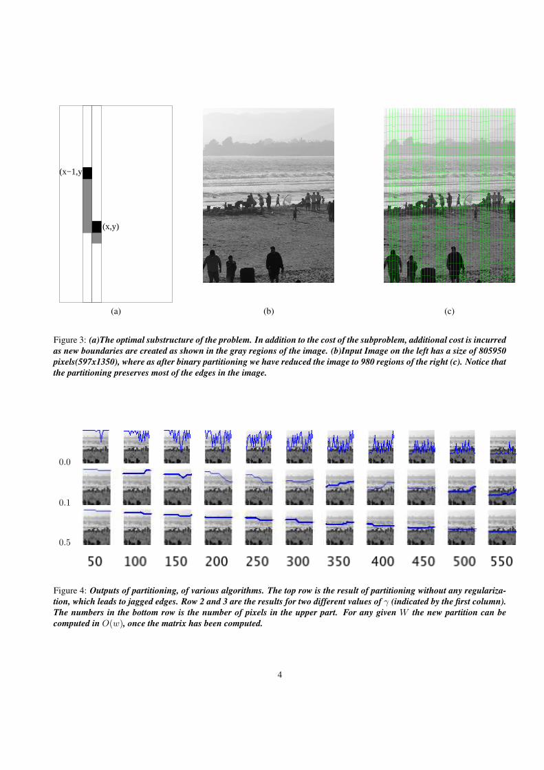
We give an algorithm for bi-partitioning the image, with theconstraint that the partition is x-monotonic, i.e, the cut in-tersects any column of the image at exactly one point. Thisis a reasonable choice for outdoor scenes like the exam-ple shown in Figure 2, where separate regions like the sky,buildings, ground, sea, etc are vertically separated. Thecomplexity of the algorithm is O(w3h2) where [w, h] is thesize of the image. This is prohibitive for large images, socan we speed up the procedure by first computing a fastpartition of the image( see Figure 3 and requiring that thecut adhere to the edges of the partitioning. This reduces thecomplexity of the algorithm to O(wh2C), where C is thenumber of regions, a speedup of O(wh
C ). An alternate ap-proach which is much easier to implement is to compute thepartition for a lower resolution image and then projectingthe partition back to the higher resolution image by linearlyinterpolating the cut. If the s is the scale of the larger imagewith respect to the smaller one, i.e. s = Worig
Wscaledthen com-
puting the partition on the smaller image and re projectinghas a speed up of s5.
We can exploit the x-monotonic structure to formulate adynamic programming approach for this problem. The par-tition is uniquely represented by the choices of y′s at eachx. Thus the problem is to compute the optimal vector y. LetI(x) denote the subimage of I which has the first x columnsof I . Let c(w, x, y) be the optimal cost of x-monotonic par-tition of I(x) ending at row y on the last column such thatthe size of the upper partition is exactly w. The notion ofupper and lower is well defined as the cut intersects the yaxis exactly once at any x. Given a contrast function δ, the
2

recurrence relations for c(w, x, y) can be written as:
c(w, x, y) = maxy′{c(w − y′, x− 1, y′)+ δ(I(x, y), I(x, y + 1))
+max(y,y′)∑
z=min(y,y′)
δ(I(x− 1, z), I(x, z))}
The boundary conditions are
c(w, 1, y) =
{−∞ if y 6= w,δ(I(1, y), I(1, y + 1)) if y = w.
The working of the algorithm is illustrated in Figure 3.The summation denoted by V (x, y, y′), can be computed inO(1) time if we precompute the sum of differences of pix-els, i.e., D(x, y) denotes the
∑yz=1 δ(I(x − 1, z), I(x, z)).
This is due to the fact that
V (x, y, y′) =max(y,y′)∑
z=min(y,y′)
δ(I(x− 1, z), I(x, z))
= D(x,max(y, y′)−D(x, min(y, y′))
D can be computed in one pass over the image.To solve theproblem we have to look for the max value of c(w′, w, h′)where w′ ∈ {W, . . . , N −W} and h′ ∈ {1, . . . , h}. Thuseach of the entries can be computed in O(h) time leadingto an overall complexity of O(w2h3). In case the image ispartitioned then we have to only compute O(NC) entries,with requiring a time of O(wh2C).
In practice however the cut resulting from this leads tovery jagged edges. This is because large difference in theadjacent positions of the vector y, leads to a larger bound-ary and hence a higher value of the function c. To preventthis we add a regularization term to the cut, which ensuressmoothness. The smoothness cost for a cut y, is given by
S(γ, y) =w∑
i=2
γ ∗ (yi − yi−1)2
The term γ, is a trade off between the smoothness and thecontrast. The optimal regularized cut can still can be com-puted by dynamic programming by observing that the regu-larized cost cr function can computed recursively in a man-ner similar to c as follows:
cr(w, x, y) = maxy′{cr(w − y′, x− 1, y′)+ δ(I(x, y), I(x, y + 1)) + V (x, y, y′)− γ ∗ (y − y′)2}
Different low level features can be taken into account forcomputing the contrast function δ between the adjacent pix-els. For the implementation we use δ(x, y) = |x − y|, i.e.difference in intensity values. One may also combine tex-ture which can be measured as the response to DOOG filters[12] at various orientation and scales. Cuts obtained for var-ious values of W and γ are shown in Figure 4. The imageis rescaled to about 1000 pixels, and an implementation inMATLAB takes about a minute to compute the matrix cr
for a given value of γ.
3 Image EnhancementWe look at the problem of enhancing grayscale images.Color images can be enhanced by extracting the luminos-ity channel of the image and enhancing it separately. Weuse histogram equalization of local regions obtained in theprevious step.
The result of histogram equalization on the global imageand the local image is shown in Figure 5. Though the localalgorithm improves the contrast better it leads to a visibleedge along the boundary of the two regions, which is highlyundesirable. Simple bilinear interpolation does not reducethe artifact much, hence we use a simple scheme of assign-ing a grayscale value as a weighted sum of its earlier colorand the new color estimated by histogram normalization.
If (x, y) = Io(x, y) ∗ w + Ie(x, y) ∗ (1− w), w ∈ [0,1]
Where If , Io, Ie is the final, original and enhancedgrayscale values respectively. The weight, w for each pixelis 1 at the boundary and 0 far away from it. We model it us-ing a gaussian function centered on the boundaries. Figure5 shows the result of enhancing the input image.
4 ConclusionIn this work we show how one can combine techniques ofsegmentation and image enhancement to contrast enhancegrayscale images with high dynamic range. The specialcase where the partitions are required to be x-monotonic hasa efficient algorithm. Though the final results are visuallygood, qualitatively measuring the performance of variousalgorithms is hard due to the lack of a well defined criteriaof performance.
References[1] Bui, T. N., and Jones, C. (1992), “Finding good ap-
proximate vertex and edge partitions is NP-hard”, In-form. Process. Lett. 42, 153-159.
3
(x−1,y)
(x,y)
(a) (b) (c)
Figure 3: (a)The optimal substructure of the problem. In addition to the cost of the subproblem, additional cost is incurredas new boundaries are created as shown in the gray regions of the image. (b)Input Image on the left has a size of 805950pixels(597x1350), where as after binary partitioning we have reduced the image to 980 regions of the right (c). Notice thatthe partitioning preserves most of the edges in the image.
0.0
0.1
0.5
Figure 4: Outputs of partitioning, of various algorithms. The top row is the result of partitioning without any regulariza-tion, which leads to jagged edges. Row 2 and 3 are the results for two different values of γ (indicated by the first column).The numbers in the bottom row is the number of pixels in the upper part. For any given W the new partition can becomputed in O(w), once the matrix has been computed.
4
(a) (b) (c)
(d) (e) (f)
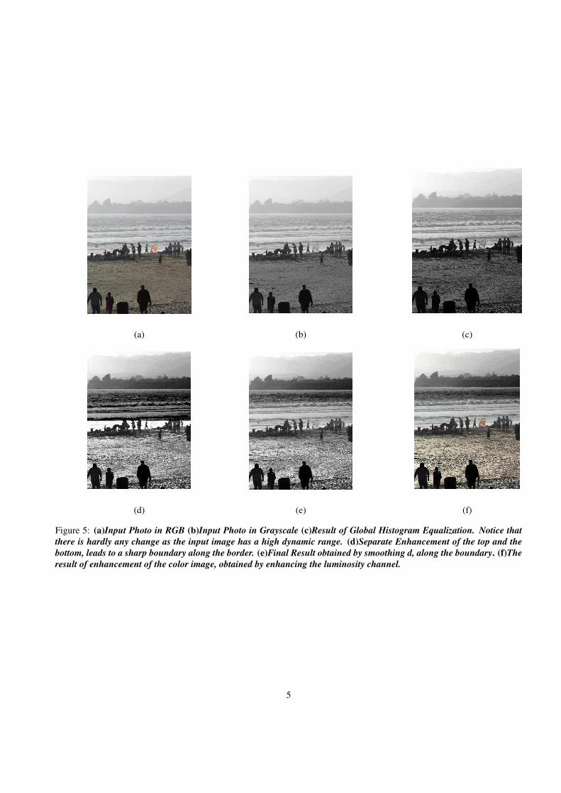
Figure 5: (a)Input Photo in RGB (b)Input Photo in Grayscale (c)Result of Global Histogram Equalization. Notice thatthere is hardly any change as the input image has a high dynamic range. (d)Separate Enhancement of the top and thebottom, leads to a sharp boundary along the border. (e)Final Result obtained by smoothing d, along the boundary. (f)Theresult of enhancement of the color image, obtained by enhancing the luminosity channel.
5
[2] Garg, N., Saran, H., and Vazirani, V. (1994), “Findingseparator cuts in planar graphs within twice the opti-mal”, Proc. 35th Ann. IEEE Symp. on Foundations ofComput. Sci., IEEE Computer Society, 14-23.
[3] Thomas H. Cormen, Charles E. Leiserson, RonaldL. Rivest, and Clifford Stein. Introduction to Algo-rithms, Second Edition. MIT Press and McGraw-Hill,2001. ISBN 0-262-03293-7. Section 26.2: The Ford-Fulkerson method, pp.651-664.
[4] W. Shih, S. Wu, and Y. Kuo. Unifying maximum cutand minimum cut of a planar graph. IEEE Trans. Com-puters, 39(5):694-697, 1990.
[5] Jianbo Shi and Jitendra Malik, ”Normalized Cuts andImage Segmentation”, IEEE Transactions on PatternAnalysis and Machine Intelligence, 22(8), 888-905,August 2000.
[6] Richard M. Karp. Reducibility Among CombinatorialProblems. In Complexity of Computer Computations,Proc. Sympos. IBM Thomas J. Watson Res. Center,Yorktown Heights, N.Y.. New York: Plenum, p.85-103. 1972.
[7] F. Hadlock, Finding a Maximum Cut of a PlanarGraph in Polynomial Time, SIAM, vol.4, no.3,p.221-225
[8] Morrow, W.M.; Paranjape, R.B.; Rangayyan, R.M.;Desautels, J.E.L. ”Region-based contrast enhance-ment of mammograms”, Medical Imaging, IEEETransactions on, Vol.11, Iss.3, Sep 1992 Pages:392-406
[9] Sakreya. Chitwong, Fusak Cheevasuvit, Kobchai De-jhan and Somsak Mitatha, ”Color Image Enhancementbased on Segmentation Region Histogram Equaliza-tion”,
[10] Digital Image Processing, Rafael C. Gonzalez ,Richard E. Woods, Addison-Wesley Pub (Sd); 3r.e.edition (March 1992)
[11] Two-Dimensional Signal and Image Processing, J. S.Lim, Prentice Hall, 1990
[12] J. Malik and P. Perona, Preattentive Texture Discrimi-nation with Early Vision Mechanisms, J. Optical Soc.Am., vol. 7, no. 2, pp. 923-932, May 1990.
6