Automatic Generation of Models of Microarchitectures
198
Automatic Generation of Models of Microarchitectures Dissertation zur Erlangung des Grades des Doktors der Ingenieurwissenschaften der Fakultät für Mathematik und Informatik der Universität des Saarlandes von Andreas Abel Saarbrücken 2020
Transcript of Automatic Generation of Models of Microarchitectures

Automatic Generation ofModels of Microarchitectures
Dissertation
zur Erlangung des Gradesdes Doktors der Ingenieurwissenschaften
der Fakultät für Mathematik und Informatikder Universität des Saarlandes
vonAndreas Abel
Saarbrücken2020

Tag des Kolloquiums: 12. Juni 2020
Dekan: Prof. Dr. Thomas Schuster
Prüfungsausschuss:
Vorsitzender: Prof. Dr. Thorsten Herfet
Berichterstatter: Prof. Dr. Jan ReinekeProf. Dr. Wolfgang J. PaulDr. Boris Köpf
Akademischer Mitarbeiter: Dr. Roland Leißa

Abstract
Detailed microarchitectural models are necessary to predict, explain, oroptimize the performance of software running on modern microprocessors.Building such models often requires a significant manual effort, as the docu-mentation provided by hardware manufacturers is typically not precise enough.The goal of this thesis is to develop techniques for generating microarchitec-tural models automatically.
In the first part, we focus on recent x86 microarchitectures. We implementa tool to accurately evaluate small microbenchmarks using hardware per-formance counters. We then describe techniques to automatically generatemicrobenchmarks for measuring the performance of individual instructionsand for characterizing cache architectures. We apply our implementations tomore than a dozen different microarchitectures.
In the second part of the thesis, we study more general techniques to obtainmodels of hardware components. In particular, we propose the concept ofgray-box learning, and we develop a learning algorithm for Mealy machinesthat exploits prior knowledge about the system to be learned.
Finally, we show how this algorithm can be adapted to minimize incompletelyspecified Mealy machines—a well-known NP-complete problem. Our imple-mentation outperforms existing exact minimization techniques by severalorders of magnitude on a number of hard benchmarks; it is even competitivewith state-of-the-art heuristic approaches.


Zusammenfassung
Zur Vorhersage, Erklärung oder Optimierung der Leistung von Software aufmodernen Mikroprozessoren werden detaillierte Modelle der verwendetenMikroarchitekturen benötigt. Das Erstellen derartiger Modelle ist oft miteinem hohen Aufwand verbunden, da die erforderlichen Information von denProzessorherstellern typischerweise nicht zur Verfügung gestellt werden. DasZiel der vorliegenden Arbeit ist es, Techniken zu entwickeln, um derartigeModelle automatisch zu erzeugen.
Im ersten Teil beschäftigen wir uns mit aktuellen x86-Mikroarchitekturen.Wir entwickeln zuerst ein Tool, das kleine kleine Microbenchmarks mithilfevon Performance Countern auswerten kann. Danach beschreiben wir Tech-niken, um automatisch Microbenchmarks zu erzeugen, mit denen die Leistungeinzelner Instruktionen gemessen sowie die Cache-Architektur charakterisiertwerden kann.
Im zweiten Teil der Arbeit betrachten wir allgemeinere Techniken, um Hard-waremodelle zu erzeugen. Wir schlagen das Konzept des “Gray-Box Learning”vor, und wir entwickeln einen Lernalgorithmus für Mealy-Maschinen, derbekannte Informationen über das zu lernende System berücksichtigt.
Zum Abschluss zeigen wir, wie dieser Algorithmus auf das Problem derMinimierung unvollständig spezifizierter Mealy-Maschinen übertragen werdenkann. Hierbei handelt es sich um ein bekanntes NP-vollständiges Problem.Unsere Implementierung ist in mehreren Benchmarks um Größenordnungenschneller als vorherige Ansätze.


Acknowledgements
First and foremost, I would like to thank my advisor, Prof. Jan Reineke.He gave me the freedom to explore my own ideas and was always availablefor discussions and to provide guidance. I’m looking forward to continuingworking with him!
I would also like to thank Prof. Wolfgang Paul and Dr. Boris Köpf for reviewingmy thesis, and Prof. Thorsten Herfet for acting as the chair of the examinationboard.
Finally, I would like to thank my current and former colleagues at the Real-Time and Embedded Systems Lab and the Compiler Design Lab. In particular,I would like to thank Dr. Roland Leißa for serving as the academic assistanton my examination board.


Contents
1 Introduction 131.1 Contributions and Structure of This Thesis . . . . . . . . . . . 141.2 Publications . . . . . . . . . . . . . . . . . . . . . . . . . . . . 19
2 nanoBench: A Low-Overhead Tool for Running Microbench-marks on x86 Systems 212.1 Introduction . . . . . . . . . . . . . . . . . . . . . . . . . . . . 212.2 Background . . . . . . . . . . . . . . . . . . . . . . . . . . . . 23
2.2.1 Hardware Performance Counters . . . . . . . . . . . . . 232.2.2 Assembler Instructions . . . . . . . . . . . . . . . . . . 25
2.3 Features . . . . . . . . . . . . . . . . . . . . . . . . . . . . . . 252.3.1 Example . . . . . . . . . . . . . . . . . . . . . . . . . . 262.3.2 Generated Code . . . . . . . . . . . . . . . . . . . . . . 272.3.3 Running the Generated Code . . . . . . . . . . . . . . 272.3.4 Kernel/User Mode . . . . . . . . . . . . . . . . . . . . 292.3.5 Interface . . . . . . . . . . . . . . . . . . . . . . . . . . 292.3.6 Loops vs. Unrolling . . . . . . . . . . . . . . . . . . . . 292.3.7 Accessing Memory . . . . . . . . . . . . . . . . . . . . 302.3.8 Warm-Up Runs . . . . . . . . . . . . . . . . . . . . . . 302.3.9 noMem Mode . . . . . . . . . . . . . . . . . . . . . . . 302.3.10 Performance Counter Configurations . . . . . . . . . . 312.3.11 Execution Time of nanoBench . . . . . . . . . . . . . . 312.3.12 Supported Platforms . . . . . . . . . . . . . . . . . . . 32
2.4 Implementation . . . . . . . . . . . . . . . . . . . . . . . . . . 322.4.1 Accurate Performance Counter Measurements . . . . . 322.4.2 Generating Code . . . . . . . . . . . . . . . . . . . . . 332.4.3 Kernel Module . . . . . . . . . . . . . . . . . . . . . . 342.4.4 Allocating Physically-Contiguous Memory . . . . . . . 34
2.5 Related Work . . . . . . . . . . . . . . . . . . . . . . . . . . . 352.6 Conclusions and Future Work . . . . . . . . . . . . . . . . . . 36
3 uops.info: Characterizing the Latency, Throughput, andPort Usage of Instructions on x86 Microarchitectures 393.1 Introduction . . . . . . . . . . . . . . . . . . . . . . . . . . . . 403.2 Related Work . . . . . . . . . . . . . . . . . . . . . . . . . . . 42
3.2.1 Information Provided by the Manufacturers . . . . . . 423.2.2 Measurement-Based Approaches . . . . . . . . . . . . . 43
3.3 Background . . . . . . . . . . . . . . . . . . . . . . . . . . . . 44
9
CONTENTS
3.3.1 Pipeline of Intel Core CPUs . . . . . . . . . . . . . . . 443.3.2 Pipeline of AMD Ryzen CPUs . . . . . . . . . . . . . . 46
3.4 Definitions . . . . . . . . . . . . . . . . . . . . . . . . . . . . . 463.4.1 Latency . . . . . . . . . . . . . . . . . . . . . . . . . . 473.4.2 Throughput . . . . . . . . . . . . . . . . . . . . . . . . 473.4.3 Port Usage . . . . . . . . . . . . . . . . . . . . . . . . 48
3.5 Algorithms . . . . . . . . . . . . . . . . . . . . . . . . . . . . . 493.5.1 Port Usage . . . . . . . . . . . . . . . . . . . . . . . . 493.5.2 Latency . . . . . . . . . . . . . . . . . . . . . . . . . . 523.5.3 Throughput . . . . . . . . . . . . . . . . . . . . . . . . 59
3.6 Implementation . . . . . . . . . . . . . . . . . . . . . . . . . . 613.6.1 Details of the x86 Instruction Set . . . . . . . . . . . . 613.6.2 Measurements on the Hardware . . . . . . . . . . . . . 623.6.3 Analysis Using IACA . . . . . . . . . . . . . . . . . . . 633.6.4 Machine-Readable Output . . . . . . . . . . . . . . . . 63
3.7 Evaluation . . . . . . . . . . . . . . . . . . . . . . . . . . . . . 633.7.1 Experimental Setup . . . . . . . . . . . . . . . . . . . . 643.7.2 Hardware Measurements vs. Documentation . . . . . . 643.7.3 Hardware Measurements vs. IACA . . . . . . . . . . . 673.7.4 Interesting Results . . . . . . . . . . . . . . . . . . . . 69
3.8 Limitations . . . . . . . . . . . . . . . . . . . . . . . . . . . . 763.9 Conclusions and Future Work . . . . . . . . . . . . . . . . . . 77
4 Characterizing Cache Architectures 794.1 Introduction . . . . . . . . . . . . . . . . . . . . . . . . . . . . 794.2 Background . . . . . . . . . . . . . . . . . . . . . . . . . . . . 81
4.2.1 Cache Organization . . . . . . . . . . . . . . . . . . . . 814.2.2 Replacement Policies . . . . . . . . . . . . . . . . . . . 82
4.3 Cache-Characterization Tools . . . . . . . . . . . . . . . . . . 864.3.1 CacheInfo . . . . . . . . . . . . . . . . . . . . . . . . . 864.3.2 CacheSeq . . . . . . . . . . . . . . . . . . . . . . . . . 884.3.3 Replacement Policies . . . . . . . . . . . . . . . . . . . 904.3.4 Age Graphs . . . . . . . . . . . . . . . . . . . . . . . . 924.3.5 Test for Adaptive Policies . . . . . . . . . . . . . . . . 92
4.4 Results . . . . . . . . . . . . . . . . . . . . . . . . . . . . . . . 944.4.1 L1 Data Caches . . . . . . . . . . . . . . . . . . . . . . 944.4.2 L2 Caches . . . . . . . . . . . . . . . . . . . . . . . . . 964.4.3 L3 Caches . . . . . . . . . . . . . . . . . . . . . . . . . 1044.4.4 Resetting the Replacement Policy State . . . . . . . . . 1094.4.5 Implementation Costs . . . . . . . . . . . . . . . . . . 111
4.5 Related Work . . . . . . . . . . . . . . . . . . . . . . . . . . . 111
10

CONTENTS
4.5.1 Microbenchmark-Based Cache Analysis . . . . . . . . . 1114.5.2 Influence of the Replacement Policy on Performance
Prediction Accuracy . . . . . . . . . . . . . . . . . . . 1134.5.3 Security Aspects of Replacement Policies . . . . . . . . 114
4.6 Conclusions and Future Work . . . . . . . . . . . . . . . . . . 115
5 Gray-Box Learning of Serial Compositions of MealyMachines 1175.1 Introduction . . . . . . . . . . . . . . . . . . . . . . . . . . . . 1185.2 Problem Statement . . . . . . . . . . . . . . . . . . . . . . . . 119
5.2.1 Basic Notions . . . . . . . . . . . . . . . . . . . . . . . 1195.2.2 The Gray-Box Learning Problem . . . . . . . . . . . . 120
5.3 Preliminaries . . . . . . . . . . . . . . . . . . . . . . . . . . . 1215.4 Approach . . . . . . . . . . . . . . . . . . . . . . . . . . . . . 122
5.4.1 Observation Tables . . . . . . . . . . . . . . . . . . . . 1235.4.2 Inference Algorithm . . . . . . . . . . . . . . . . . . . . 126
5.5 Implementation . . . . . . . . . . . . . . . . . . . . . . . . . . 1285.5.1 Computing the Partitions . . . . . . . . . . . . . . . . 1285.5.2 Reachability of the Error State . . . . . . . . . . . . . 1315.5.3 Checking if Two Machines are Right-Equivalent . . . . 1315.5.4 Handling Counterexamples . . . . . . . . . . . . . . . . 132
5.6 Evaluation . . . . . . . . . . . . . . . . . . . . . . . . . . . . . 1325.7 Related Work . . . . . . . . . . . . . . . . . . . . . . . . . . . 1345.8 Conclusions and Future Work . . . . . . . . . . . . . . . . . . 1355.A Appendix: Proofs for Chapter 5 . . . . . . . . . . . . . . . . . 136
6 MeMin: SAT-Based Exact Minimization of IncompletelySpecified Mealy Machines 1396.1 Introduction . . . . . . . . . . . . . . . . . . . . . . . . . . . . 139
6.1.1 Outline . . . . . . . . . . . . . . . . . . . . . . . . . . 1416.2 Definitions . . . . . . . . . . . . . . . . . . . . . . . . . . . . . 141
6.2.1 Basic Definitions . . . . . . . . . . . . . . . . . . . . . 1416.2.2 Problem Statement . . . . . . . . . . . . . . . . . . . . 1436.2.3 General Approach . . . . . . . . . . . . . . . . . . . . . 143
6.3 Related Work . . . . . . . . . . . . . . . . . . . . . . . . . . . 1446.4 Approach . . . . . . . . . . . . . . . . . . . . . . . . . . . . . 146
6.4.1 Incompatibility Matrix . . . . . . . . . . . . . . . . . . 1476.4.2 Encoding as a SAT Problem . . . . . . . . . . . . . . . 1476.4.3 Computing a Partial Solution . . . . . . . . . . . . . . 149
6.5 Implementation . . . . . . . . . . . . . . . . . . . . . . . . . . 1496.5.1 Dealing with Partially Specified Outputs . . . . . . . . 149
11
CONTENTS
6.5.2 Dealing with Partially Specified Inputs . . . . . . . . . 1506.5.3 Undefined Reset States . . . . . . . . . . . . . . . . . . 150
6.6 Evaluation . . . . . . . . . . . . . . . . . . . . . . . . . . . . . 1506.6.1 Benchmarks . . . . . . . . . . . . . . . . . . . . . . . . 1516.6.2 Evaluation of MeMin . . . . . . . . . . . . . . . . . . . 1556.6.3 Other Tools . . . . . . . . . . . . . . . . . . . . . . . . 1556.6.4 Experimental Setup . . . . . . . . . . . . . . . . . . . . 158
6.7 Conclusions and Future Work . . . . . . . . . . . . . . . . . . 1586.A Appendix: Complete Benchmark Results . . . . . . . . . . . . 159
7 Summary, Conclusions, and Future Work 1657.1 Summary and Conclusions . . . . . . . . . . . . . . . . . . . . 165
7.1.1 Models of Recent Microarchitectures . . . . . . . . . . 1657.1.2 General Models . . . . . . . . . . . . . . . . . . . . . . 166
7.2 Future Work . . . . . . . . . . . . . . . . . . . . . . . . . . . . 167
Bibliography 169
Index 197
12

1Introduction
Modern microprocessors are among the most complex man-made systems.As a consequence, it is becoming increasingly difficult to predict, explain, oroptimize the performance of software running on such microprocessors. As abasis, one needs detailed models of their microarchitectures.
Such models are, for example, required to build optimizing compilers, worst-case execution time (WCET) analyzers, cycle-accurate simulators, or self-optimizing software systems. Similarly, such models are necessary to showthe presence or absence of microarchitectural security issues, such as Spectreand Meltdown [KHF+19, LSG+18]. Finally, detailed knowledge of microar-chitectural details is also helpful when manually fine-tuning a piece of codefor a specific processor.
Unfortunately, the documentation provided by hardware manufacturers isusually not detailed enough. To build microarchitectural models, engineers arethus often forced to perform measurements using microbenchmarks. Existingapproaches typically require a significant amount of manual effort, and theresults are not always accurate and precise.
The goal of this thesis therefore is to develop techniques for generating detailedmodels of microarchitectures automatically.
In the first part of the thesis, we focus on recent x86 microarchitectures.In particular, we develop techniques to automatically generate models fortwo properties that have a strong influence on the performance of softwareon a specific microarchitecture: the cache architecture and the latencies,throughputs, and port usages of individual instructions.
In the second part of the thesis, we look at more general techniques forobtaining models of hardware components. Specifically, we introduce theproblem of gray-box learning, in which learning algorithms may exploit knowninformation about the system to be learned.
13

CHAPTER 1. INTRODUCTION
1.1 Contributions and Structure of This ThesisWe now describe the addressed problems, and our approaches and contribu-tions in more detail.
nanoBenchIn Chapter 2, we develop nanoBench, a tool for evaluating small microbench-marks using hardware performance counters on x86 systems. Hardwareperformance counters are special-purpose registers that store the counts ofvarious hardware-related events.
In contrast to previous tools, nanoBench can execute microbenchmarksdirectly in kernel space. This makes it possible to benchmark privilegedinstructions, and it allows for more accurate measurements by disablinginterrupts and preemptions. Furthermore, this makes it also possible todirectly access certain performance counters that are only available in kernelspace; previous tools require expensive system calls to access such counters.
nanoBench provides the option to temporarily pause performance countingduring specific parts of a microbenchmark. Furthermore, the reading ofthe performance counters is implemented with minimal overhead, avoidingfunction calls and branches. As a consequence, nanoBench is precise enoughto measure, e.g., whether individual memory accesses result in cache hits ormisses.
We use nanoBench to evaluate the microbenchmarks generated by the toolsdescribed in the following paragraphs.
Instruction CharacterizationsAn aspect that has a relatively strong influence on performance is how ISAinstructions decompose into micro-operations (µops), which ports these µopsmay be executed on, and what their latencies and throughputs are.
However, these properties are typically only poorly documented. Intel’sprocessor manuals [Int12, Int19b], for example, only contain latency andthroughput data for a number of “commonly-used instructions.” They do notcontain information on the decomposition of individual instructions into µops,nor do they state the execution ports that these µops can use.
The only way to obtain accurate instruction characterizations for many recentmicroarchitectures is thus to perform measurements using microbenchmarks.
14

1.1. CONTRIBUTIONS AND STRUCTURE OF THIS THESIS
However, existing approaches, such as [Fog19], require significant manualeffort to create suitable microbenchmarks and to interpret their results.Furthermore, the results are not always accurate and precise.
In Chapter 3, we develop a new approach that can automatically generatemicrobenchmarks in order to characterize the latency, throughput, and portusage of instructions on x86 CPUs in an accurate and precise manner.
Before describing our algorithms and their implementation, we first discusscommon notions of instruction latency, throughput, and port usage. For thelatency, we propose a new definition that, in contrast to previous definitions,considers dependencies between different pairs of input and output operands,which enables more accurate performance predictions.
We then develop algorithms that generate assembler code for microbench-marks to measure the properties of interest for most x86 instructions. Ouralgorithms take into account explicit and implicit dependencies, such as, e.g.,dependencies on status flags. Therefore, they require detailed informationon the x86 instruction set. To this end, we create a machine-readable XMLrepresentation of the x86 instruction set that contains all the informationneeded to automatically generate assembler code for every instruction. Therelevant information is automatically extracted from the configuration files ofIntel’s x86 Encoder Decoder (XED) [Intc] library.
We have implemented our algorithms in a tool that we have successfullyapplied to 16 different Intel and AMD microarchitectures. The output of ourtool is available both in the form of a human-readable, interactive HTMLtable and as a machine-readable XML file, so that it can be easily usedto implement, e.g., simulators, performance prediction tools, or optimizingcompilers.
Finally, we discuss several interesting insights obtained by comparing theresults from our measurements with previously published data. Our preciselatency data, for example, uncovered previously undocumented differencesbetween different microarchitectures. It also explains discrepancies betweenpreviously published information. Apart from that, we uncovered variouserrors in Intel’s IACA tool [Inta], and inaccuracies in the manuals.
Characterizing Cache ArchitecturesTo bridge the increasing latency gap between the processor and main memory,modern microarchitectures employ memory hierarchies with multiple levelsof cache memory. These caches are small but fast memories that make use
15

CHAPTER 1. INTRODUCTION
of temporal and spatial locality. Typically, they have a big impact on theexecution time of computer programs; the penalty of a miss in the last-levelcache can be more than 200 cycles.
In Chapter 4, we develop techniques for creating models of cache architectures.We focus, in particular, on cache replacement policies, which are typicallyundocumented for recent microarchitectures.
To this end, we develop several tools for determining cache parameters. Thefirst tool, cacheInfo, provides details on the structure of the caches, suchas the sizes, the associativities, the number of cache sets, or the number ofC-Boxes and slices.
Our second tool, cacheSeq, makes it possible to analyze the behavior of thecaches by measuring the number of cache hits and misses when executing anaccess sequence in one or more cache sets; the access sequence is supplied asa parameter to the tool and can be specified using a convenient syntax. Toperform these measurements, the tool generates suitable microbenchmarksthat are evaluated using nanoBench.
Based on cacheSeq, we then develop several tools for identifying the replace-ment policy. In particular, we implement a tool that can automatically inferpermutation policies, and a tool that can automatically determine whetherthe policy belongs to a set of more than 300 variants of commonly usedpolicies, including policies like MRU and QLRU, which are not permutationpolicies. These tools are precise enough to determine the policies used inindividual cache sets. In addition to that, we develop a tool that can findout whether the cache uses an adaptive replacement policy. Furthermore, wepropose a tool that creates age graphs, which are helpful for analyzing cacheswith nondeterministic replacement policies.
We have applied our tools to 13 different Intel microarchitectures, and weprovide detailed models of their replacement policies. We have discoveredseveral previously undocumented replacement policies.
Gray-Box LearningThe algorithms we developed for Chapters 3 and 4 can be seen as instances ofactive learning approaches. Active learning (also called query learning) refersto a class of machine-learning techniques in which the learning algorithm isable to interact with the system to be learned.
However, the algorithms we developed for Chapters 3 and 4 are heavilytargeted at the specific problems. In Chapter 5, we look at more general
16

1.1. CONTRIBUTIONS AND STRUCTURE OF THIS THESIS
techniques. Specifically, we consider approaches for learning finite statemachines, which are, in principle, suitable abstractions for modeling thebehavior of microarchitectural components.
In active learning approaches, one commonly assumes an oracle, or teacher,that admits two kinds of queries about the system: output queries returnthe result of the system for a specific input, and equivalence queries checkwhether a conjectured model is consistent with the system to be learnedand return a counterexample if not. Based on this setup, Angluin intro-duced the L∗ algorithm [Ang87] for learning deterministic finite automata.L∗ has since been extended to other modeling formalisms, such as Mealy ma-chines [SG09], register automata [HSJC12, BHLM13, AFBKV15], or symbolicautomata [MM14].
As the system is usually treated as a black box, no information about theinternal structure of the system can be taken into account by most existinglearning algorithms. In practice, however, systems are often composed ofsubcomponents, for some of which models might be available, but it is notpossible to access the known and the unknown parts separately from theoutside.
While it is in theory possible to learn a model of the entire system usingexisting black-box approaches, this is often not viable in practice because thestate space is too large. A problem, which has received very little attention inthe literature so far, is how to use the available information about the systemto focus the learning algorithm on those parts that are unknown. We callthis problem gray-box learning.
As a first step toward solving this problem, we study one specific instance.We consider the serial composition of two Mealy machines A and B, where Ais known and B is unknown, and we assume that we can only perform querieson the composed machine.
While output queries can often be realized cheaply by measurements on theactual system, equivalence queries can usually only be approximated by alarge number of such measurements. Our primary focus is thus to minimizethe number of equivalence queries. We introduce an algorithm to exactlylearn B in the context of A that performs at most |B| equivalence queries,where |B| denotes the number of states of B.
We evaluate our approach on compositions of randomly-generated machinesagainst an implementation of the classic L∗ algorithm in LearnLib [IHS15].We show that our approach requires significantly fewer output and equivalencequeries on most benchmarks.
17

CHAPTER 1. INTRODUCTION
Minimization of Incompletely Specified Mealy MachinesIt is generally a desirable property of models to be as small as possible.In Chapter 6, we take a fresh look at the problem of minimizing incom-pletely specified Mealy machines, i.e., machines where one or more outputsor next states might not be specified. While the minimization problem isefficiently solvable for fully specified machines [Hop71], it is NP-complete forincompletely specified ones [Pfl73].
It turns out that this problem is quite closely related to the gray-box learninginstance we studied in Chapter 5. A central algorithmic idea of our learningtechnique is a reduction to a Boolean satisfiability (SAT) problem. In Chap-ter 6, we show how a relatively straightforward adaptation of this reductionapproach can be used to minimize incompletely specified Mealy machines.
The minimization problem has been extensively studied before, and a numberof exact and heuristic approaches have been proposed. We compare animplementation of our exact approach to several other approaches on twosets of standard benchmarks.
Our approach outperforms the other exact approaches significantly, in partic-ular on a number of hard benchmarks. In some cases, it is faster than existingapproaches by several orders of magnitude.
On most benchmarks, our approach is also competitive with state-of-the-artheuristic methods. There are only two benchmarks on which a heuristicapproach is significantly faster. However, in these two cases, this heuristicapproach is not able to find the minimal result.
18

1.2. PUBLICATIONS
1.2 PublicationsKey parts of this thesis have been published in the following papers.
• [AR14]: Andreas Abel and Jan Reineke. Reverse engineering ofcache replacement policies in Intel microprocessors and theirevaluation. In IEEE International Symposium on Performance Anal-ysis of Systems and Software (ISPASS), Monterey, CA, USA, March23–25, 2014, pages 141–142. © 2014 IEEE
• [AR15]: Andreas Abel and Jan Reineke. MeMin: SAT-based exactminimization of incompletely specified Mealy machines. InProceedings of the IEEE/ACM International Conference on Computer-Aided Design (ICCAD), Austin, TX, USA, November 2–6, 2015, pages94–101. © 2015 IEEE
• [AR16]: Andreas Abel and Jan Reineke. Gray-box learning of serialcompositions of Mealy machines. In NASA Formal Methods—Proceedings of the 8th International Symposium, Minneapolis, MN,USA, June 7–9, 2016, pages 272–287. Springer-Verlag, 2016.
• [AR19]: Andreas Abel and Jan Reineke. uops.info: Characterizinglatency, throughput, and port usage of instructions on Intelmicroarchitectures. In Proceedings of the Twenty-Fourth Interna-tional Conference on Architectural Support for Programming Languagesand Operating Systems (ASPLOS), Providence, RI, USA, April 13–17,2019, pages 673–686. ACM, 2019.
• [AR20]: Andreas Abel and Jan Reineke. nanoBench: A low-over-head tool for running microbenchmarks on x86 systems. InIEEE International Symposium on Performance Analysis of Systemsand Software (ISPASS), Boston, MA, USA, August 23–25, 2020. Toappear. © 2020 IEEE
19


2nanoBench:
A Low-Overhead Tool for RunningMicrobenchmarks on x86 Systems
In this chapter, we present nanoBench, a tool for evaluating small micro-benchmarks using hardware performance counters on Intel and AMD x86systems. Most existing tools and libraries are intended to either benchmarkentire programs, or program segments in the context of their execution withina larger program. In contrast, nanoBench is specifically designed to evaluatesmall, isolated pieces of code. Such microbenchmarks are commonly used foranalyzing undocumented hardware properties.
Unlike previous tools, nanoBench can execute microbenchmarks directly inkernel space. This allows to benchmark privileged instructions, and it enablesmore accurate measurements. The reading of the performance counters isimplemented with minimal overhead, avoiding function calls and branches. Asa consequence, nanoBench is precise enough to measure individual memoryaccesses.
Most of the work presented in this chapter has been published in [AR20].
2.1 IntroductionBenchmarking small pieces of code using hardware performance countersis often useful for analyzing the performance of software on a specific mi-croprocessor, as well as for analyzing performance characteristics of themicroprocessor itself.
21
CHAPTER 2. NANOBENCH
Such microbenchmarks can, e.g., be helpful in identifying bottlenecks in loopkernels. To this end, modern x86 CPUs provide many performance eventsthat can be measured, such as cache hits and misses in different levels of thememory hierarchy, the pressure on execution ports, mispredicted branches, etc.
Low-level aspects of microarchitectures are typically only poorly documented.Thus, the only way to obtain detailed information is often through mi-crobenchmarks using hardware performance counters. This includes, forexample, the latency, throughput, and port usage of individual instructions(see Section 3.2.2). Microbenchmarks have also been used to infer propertiesof the memory hierarchy (see Section 4.5.1). In addition to that, such bench-marks have been used to identify microarchitectural properties that can leadto security issues, such as Spectre [KHF+19] and Meltdown [LSG+18].
Often, such microbenchmarks consist of two parts: The main part, and aninitialization phase that, for example, sets registers or memory locations tospecific values or tries to establish a specific microarchitectural state, e.g., byflushing the caches. Ideally, the performance counters should only be activeduring the main part.
To facilitate the use of hardware performance counters, a number of tools andlibraries have been proposed. Most of the existing tools fall into one of twocategories. First, there are tools that benchmark entire programs, such asperf [per], or profilers like Intel’s VTune Amplifier [Intb]. Tools in the secondcategory are intended to benchmark program segments that are executed in thecontext of a larger program. They usually provide functions to start and stopthe performance counters that can be called before and after the code segmentof interest. Such tools are, for example, PAPI [TJYD10] and libpfc [Bil].
Tools from both categories are not particularly well suited for microbench-marks of the kind described above. For tools from the first category, oneobvious reason is that it is not possible to measure only parts of the code.Another reason is overhead. Just running a C program with an empty mainfunction, compiled with a recent version of gcc, leads to the execution ofmore than 500,000 instructions and about 100,000 branches. Moreover, thisnumber varies significantly from one run to another.
Overhead can also be a concern for tools from the second category. InPAPI, for example, the calls to start and stop the counters involve severalhundred memory accesses, more than 150 branches, and for some counterseven expensive system calls. This leads to unpredictable execution times andmight, e.g., destroy the cache state that was established in the initializationpart of the microbenchmark. Moreover, these calls will modify general-purpose
22

2.2. BACKGROUND
registers, so it is not possible to set the registers to specific values in theinitialization part and use these values in the main part.
For several reasons, microbenchmarks often need to be run multiple times.One reason is the possibility of interference due to interrupts, preemptions orcontention on shared resources that are also used by programs on other cores.Another reason are issues such as cold caches that impact the performanceon the first runs. A third reason is that there are more performance eventsthan there are programmable counters, so the measurements may need tobe repeated with different counter configurations. Also, the code to bebenchmarked itself often needs to be repeated several times. This is typicallydone by executing it in a loop or by unrolling it multiple times, or by acombination of both. All of this leads to a significant engineering effort thatneeds to be repeated over and over again.
In this chapter, we present nanoBench1, an open-source tool that makesit very easy to evaluate small microbenchmarks on recent x86 CPUs. InChapters 3 and 4, we describe techniques to automatically generate suchmicrobenchmarks for characterizing the performance of instructions and foranalyzing properties caches.
There are two variants of our tool: A user-space implementation and a kernel-space version. The kernel-space version makes it possible to directly bench-mark privileged instructions, in contrast to any previous tool we are aware of.Furthermore, it allows for more accurate measurements than existing tools bydisabling interrupts and preemptions. The tool is precise enough to measure,e.g., whether individual memory accesses result in cache hits or misses.
Microbenchmarks may use and modify any general-purpose and vector reg-isters, including the stack pointer. After executing the microbenchmark,nanoBench automatically resets them to their previous values. The loop andunroll counts, as well as the number of repetitions and the aggregate functionto be applied to the measurement results, can be specified via parameters.
2.2 Background
2.2.1 Hardware Performance CountersRecent Intel and AMD processors are equipped with different types of hard-ware performance counters, i.e., special-purpose registers that store the countsof various hardware-related events. All of these counters can be read using
1https://github.com/andreas-abel/nanoBench
23

CHAPTER 2. NANOBENCH
the RDMSR2 instruction; many of them can also be read using the RDPMC 3
instruction. The RDMSR instruction is a privileged instruction and can, thus,only be used in kernel space. The RDPMC instruction, on the other hand, isfaster than the RDMSR instruction, and it can be directly accessed in userspace if a specific flag in a control register is set.
Core Performance Counters
Each logical core has a private performance monitoring unit with multipleperformance counters. There are two types of core performance counters:
• Fixed-Function Performance Counters
Recent Intel CPUs have three fixed-function performance counters thatcan be read with the RDPMC instruction. They count the numberof retired instructions, the number of core cycles, and the number ofreference cycles.
In addition to that, there are two fixed-function counters that areavailable both on recent Intel CPUs, as well as on AMD family 17hCPUs: the APERF counter, which counts core clock cycles, and theMPERF counter, which counts reference cycles. These two counterscan only be accessed with the RDMSR instruction and are, thus, onlyavailable in kernel space.
• Programmable Performance Counters
Recent Intel CPUs have between two and eight, and AMD family 17hCPUs have six programmable performance counters. They can beprogrammed with a large number of different performance events (morethan 200 on some CPUs), such as the number of µops that use a specificport, the number of cache misses in different levels of the memoryhierarchy, the number of mispredicted branches, etc. These counterscan be read with the RDPMC instruction.
Uncore/L3 Performance Counters
In addition to the per-core performance counters described above, recentprocessors also have a number of programmable global performance countersthat can, in particular, count events related to the shared L3 caches. On IntelCPUs, these counters can only be read in kernel space.
2“Read from model specific register”3“Read performance-monitoring counters”
24

2.3. FEATURES
2.2.2 Assembler InstructionsThroughout this thesis, we use assembler instructions in Intel syntax. Theyhave the following form:
mnemonic op1, op2, ...
The mnemonic identifies the operation, e.g., ADD or XOR. The first operandop1 is typically the destination operand, and the other operands are thesource operands (an operand can also be both a source and destinationoperand). Operands can be registers, memory locations, or immediates.Memory operands use the syntax
[Rbase+Rindex*scale+disp],
where Rbase and Rindex are general-purpose registers, disp is an integer, andscale is 1, 2, 4, or 8. All of these components are optional and can be omitted.
In addition to these explicit operands, an instruction can also have implicitoperands. As an example, consider the following instruction:
ADD RAX, [RBX]
This instruction computes the sum of the general-purpose register RAX and thememory at the address of register RBX, and stores the result in RAX. We referto RAX and [RBX] as explicit operands. In addition to that, the instructionupdates the status flags (e.g., the carry flag) according to the result. Thestatus flags are implicit operands of the ADD instruction.
There are often multiple variants of an instruction with different operandtypes and/or widths.
Note that there is not always a one-to-one correspondence between assemblercode and machine code. Sometimes, there are multiple possible encodings forthe same assembler instruction. It is, in general, not possible to control whichof these encodings the assembler selects. Thus, some machine instructionscannot be generated using assembler code.
2.3 FeaturesIn this section, we first give a high-level overview by looking at a simpleexample that shows how nanoBench can be used. We then describe variousfeatures of nanoBench in more detail.
25

CHAPTER 2. NANOBENCH
2.3.1 ExampleThe following example shows how nanoBench can be used to measure thelatency of the L1 data cache on a Skylake-based system.
./nanoBench.sh -asm "mov R14, [R14]"-asm_init "mov [R14], R14"-config cfg_Skylake.txt
The tool will first execute the instruction
mov [R14], R14,
which copies the value of register R14 to the memory location that R14 pointsto. nanoBench always initializes R14 (and a number of other registers) to pointinto a dedicated memory area that can be freely modified by microbenchmarks;this is described in more detail in Section 2.3.7.
nanoBench then starts the performance counters and executes the instruction
mov R14, [R14]
multiple times. The number of repetitions can be controlled via parameters;for more information see Section 2.3.6. The instruction loads the value atthe address in R14 into R14. Thus, the execution time of this instructioncorresponds to the L1 data cache latency. Afterwards, nanoBench stops theperformance counters. The entire benchmark is then repeated multiple timesto obtain stable results.
The output of nanoBench will be similar to the following:
Instructions retired: 1.00Core cycles: 4.00Reference cycles: 3.52UOPS_ISSUED.ANY: 1.00UOPS_DISPATCHED_PORT.PORT_0: 0.00UOPS_DISPATCHED_PORT.PORT_1: 0.00UOPS_DISPATCHED_PORT.PORT_2: 0.50UOPS_DISPATCHED_PORT.PORT_3: 0.50UOPS_DISPATCHED_PORT.PORT_4: 0.00UOPS_DISPATCHED_PORT.PORT_5: 0.00MEM_LOAD_RETIRED.L1_HIT: 1.00MEM_LOAD_RETIRED.L2_HIT: 0.00MEM_LOAD_RETIRED.L3_HIT: 0.00MEM_LOAD_RETIRED.L3_MISS: 0.00
26

2.3. FEATURES
The first three lines show the result of the fixed-function performance counters.The remaining lines correspond to the performance events specified in thecfg_Skylake.txt configuration file that was supplied as a parameter in thenanoBench call shown above; details on configuration files are described inSection 2.3.10.
From the results, we can conclude that the L1 data cache latency is 4 cycles.This agrees with the documentation in Intel’s optimization manual [Int19b].
2.3.2 Generated CodeTo execute a microbenchmark, nanoBench first generates code for a functionsimilar to the pseudocode shown in Algorithm 2.1.
In line 2, the generated code first saves the current values of the registers to thememory and initializes certain registers to point to specific memory locations(see Section 2.3.7). Then, the initialization part of the microbenchmark isexecuted (line 3). In the next line (line 4), the performance counters are read.Unless the noMem option (see Section 2.3.9) is used, this step does not modifythe values in any general-purpose or vector registers that were set by theinitialization code (technically, it does modify certain registers temporarily,but it resets them to their previous value before the next line is executed).
Lines 5 to 9 contain the code for the main part of the microbenchmark. Thecode is unrolled multiple times (this can be configured via a parameter, seeSection 2.3.6). If the parameter loopCount is larger than 0, the code for afor-loop is inserted in line 5; in this case, the code of the microbenchmarkmust not modify register R15, which is used to store the loop counter.
Afterwards, the performance counters are read a second time (line 10), andin line 11, the registers are restored to the values that were saved in line 2.Finally, the difference between the two performance counter values, dividedby the number of repetitions, is returned.
2.3.3 Running the Generated CodeAlgorithm 2.2 shows how the generated code is run. The code is run aconfigurable number of times. At the end, an aggregate function is appliedto the measurement results, which can be either the minimum, the median,or the arithmetic mean (excluding the top and bottom 20% of the values).A configurable number of runs in the beginning can be excluded from theresult; this is described in more detail in Section 2.3.8.
27

CHAPTER 2. NANOBENCH
By default, nanoBench generates and runs two versions of the code: the firstone with localUnrollCount set to the specified unrollCount, and the secondtime with localUnrollCount set to two times the specified unrollCount. Thereported result is the difference between the two runs. This removes theoverhead of the measurement instructions from the result, as well as anomaliesthat might be caused by the serialization instructions that are needed beforeand after reading the performance counters (see also Section 2.4.1).
nanoBench also provides an option that uses a localUnrollCount of 0 for oneof the runs instead (i.e., there are no instructions between line 4 and line 10in this case).
Algorithm 2.1: Generated code for a microbenchmark1 Function generatedCode()2 saveRegs3 codeInit4 m1← readPerfCtrs // stores results in memory,
// does not modify registers5 for j ← 0 to loopCount do // this line is omitted
// if loopCount=06 code // copy #17 code // copy #2
8...
9 code // copy #localUnrollCount
10 m2← readPerfCtrs11 restoreRegs12 r ← (m2−m1)/(max(1, loopCount) ∗ localUnrollCount)13 return r
Algorithm 2.2: Running a microbenchmark1 Function run(code)2 for i← −warmUpCount to nMeasurements do3 m← code()4 if i ≥ 0 then // ignore warm-up runs5 measurements [i]← m
6 return agg(measurements) // apply aggregate function
28

2.3. FEATURES
2.3.4 Kernel/User ModenanoBench is available in two versions: A user-space and a kernel-spaceversion. The kernel-space version has several advantages over the user-spaceversion:
• It makes it possible to benchmark privileged instructions.
• It can allow for more accurate measurement results as it disables inter-rupts and preemptions during measurements.
• It can use several performance counters that are not accessible fromuser space, like the uncore counters on Intel CPUs, or the APERF andMPERF counters.
• It can allocate physically-contiguous memory. See also Section 2.3.7.
On the other hand, executing microbenchmarks in kernel space can lead topotential data loss and security problems if the microbenchmarks contain bugs.It is thus recommended to use the kernel-space version only on dedicated testmachines.
2.3.5 InterfaceWe provide a unified interface to the user-space and the kernel-space versionin the form of two shell scripts, nanoBench.sh and kernel-nanoBench.sh,that have mostly the same command-line options.
In addition to that, we also provide a Python interface for the kernel-spaceversion. This interface is used for the tools described in Chapters 3 and 4.
With all interfaces, the code of the microbenchmarks can be specified ei-ther as an assembler code sequence in Intel syntax (like in the example inSection 2.3.1), or by the name of a binary file containing x86 machine code.
2.3.6 Loops vs. UnrollingFor microbenchmarks that have code that needs to be repeated several timesto obtain meaningful results, there is a trade-off between unrolling the code(i.e., creating multiple copies of it) and executing the code in a loop.
Using a loop has the advantage of keeping the code size small, so that itwill fit into the cache. On the other hand, the loop introduces an additionaloverhead, which can be significant if the body of the loop is small.
29

CHAPTER 2. NANOBENCH
Whether unrolling or a loop should be used, depends on the particularbenchmark. For benchmarks that measure, e.g., the number of data cachemisses, a loop is the better choice, as it does not introduce any overhead interms of memory accesses. On the other, for a benchmark that measures theport usage of an instruction, using only unrolling is better, as otherwise, theµops of the loop code compete for ports with the µops of the benchmark. Forsome benchmarks, a combination of both a loop and unrolling yields the bestresults.
nanoBench provides two parameters, loopCount and unrollCount, that controlthe number of loop iterations, and how often the code is unrolled.
2.3.7 Accessing MemorynanoBench initializes the registers RSP (i.e., the stack pointer), RBP (i.e., thebase pointer), RDI, RSI, and R14 to point into dedicated memory areas (of1MB each) that can be freely modified by the microbenchmarks.
Furthermore, for microbenchmarks needing a larger memory area, like bench-marks for determining cache parameters, the kernel version of nanoBenchprovides an option for reserving a physically-contiguous memory area of aconfigurable size (see also Section 2.4.4).
2.3.8 Warm-Up RunsnanoBench provides the option of performing a configurable number of initialbenchmark runs that are excluded from the results. This can, for example,be useful to make sure that the code and other accessed memory locationsare in the cache. It can also be used to train the branch predictor toreduce the number of mispredicted branches. Furthermore, there are someinstructions that require a warm-up period after having not been used for awhile before they can execute at full speed again, like AVX2 instructions onsome microarchitectures.
2.3.9 noMem ModeBy default, the code to read the performance counters writes the results tothe memory. After a warm-up run, this memory location is usually in thecache, and thus, the time for these memory operations is constant.
However, for microbenchmarks that contain many memory accesses to differentaddresses that map to the same cache set, writing the performance counter
30

2.3. FEATURES
results to the memory can be problematic. One reason for this is that thememory accesses in line 4 may change a cache state that was establishedby the initialization part of the benchmark. Another reason is that themicrobenchmark code may evict the block that stores the performance counterresults, which would lead to additional cache misses.
To avoid these problems, nanoBench has a special mode that stores allperformance counter measurements in registers instead of in memory. If thismode is used, certain general-purpose registers must not be modified by themicrobenchmark.
Moreover, if this mode is used, nanoBench also provides a feature to tem-porarily pause performance counting. This feature can be used by includingspecial magic byte sequences in the microbenchmark code for stopping andresuming performance counting. Using this feature incurs a certain timingoverhead, so it is in particular useful for benchmarks that do not measure thetime but, e.g., the number of cache hits or misses.
2.3.10 Performance Counter ConfigurationsThe performance events to be measured are specified in a configuration file.The file uses a simple syntax to define the events. Unlike in some previoustools, like libpfc [Bil], the events are not hard-coded, which makes it easy toadapt nanoBench to future CPUs, as only a new configuration file has to becreated.
If the configuration file contains more events than there are programmableperformance counters, the benchmarks are automatically executed multipletimes with different counter configurations.
We provide configuration files with all events for all recent Intel microarchi-tectures and the AMD Zen microarchitecture.
2.3.11 Execution Time of nanoBenchEvaluating microbenchmarks with nanoBench is very fast. As an example, weconsider a benchmark consisting of a single NOP instruction, that is run withunrollCount = 100, loopCount = 0, nMeasurements = 10, and a configurationfile with four events. On an Intel Core i7-8700K, running nanoBench withthese parameters takes about 15ms for the kernel version (assuming that thekernel module is already loaded), and about 50ms for the user-space version.
31

CHAPTER 2. NANOBENCH
2.3.12 Supported PlatformsWe have successfully used nanoBench on processors from most generations ofIntel’s Core microarchitecture and with AMD Ryzen CPUs. All experimentswere performed under Ubuntu 18.04, but nanoBench should be compatiblewith any Linux distribution that uses a recent kernel version.
2.4 Implementation
2.4.1 Accurate Performance Counter MeasurementsSerializing Instruction Execution
As described in Section 2.2, performance counters can be read with theRDPMC or the RDMSR instruction. These instructions are not serializinginstructions. Thus, due to out-of-order execution (see Section 3.3), they maybe reordered with earlier or later instructions by the processor. For obtainingmeaningful measurement results, it is therefore important to add instructionsthat serialize the instruction stream both before and after any instructionsthat read performance counters.
Previous approaches (e.g., [Fog]) often use the CPUID instruction for thatpurpose. However, for benchmarking short code segments, this is problematic.One reason for this is that the CPUID instruction has a variable latency andµop count. Paoloni [Pao10] observed that the execution time of the CPUIDcan differ by hundreds of cycles from run to run. The variable µop countcan be eliminated by setting the register RAX to a fixed value before eachexecution of the CPUID instruction; this also reduces the variance in theexecution time, but does not fully eliminate it. Moreover, for an instructionsequence of the form
A; CPUID; B,
the serialization property of the CPUID instruction only guarantees thatall µops of A have completed before B is fetched and executed. It does notguarantee that all µops of A have completed before the first µop of the CPUIDinstruction is executed, and it does also not guarantee that all µops of theCPUID instruction have completed before the first µop of B is executed.
We propose to use the LFENCE instruction instead. This instruction isnot fully serializing: it does not guarantee that earlier stores have becomeglobally visible, and subsequent instructions may be fetched from memorybefore LFENCE completes. However, on Intel CPUs it does guarantee that
32

2.4. IMPLEMENTATION
“LFENCE does not execute until all prior instructions have completed locally,and no later instruction begins execution until LFENCE completes” [Int19c].For our purposes, this is sufficient, and the guarantee is even somewhatstronger than that for the CPUID instruction, as it also orders the LFENCEinstruction itself with respect to the preceding and succeeding instructions. OnAMD CPUs, the LFENCE provides similar guarantees if Spectre mitigationsare enabled. Using the LFENCE instruction for measurements of shortdurations was also recently recommended by McCalpin [McC18].
Reducing Interference
In the kernel-space version, we disable preemptions and hard interrupts duringmeasurements, as they can perturb the measurement results [WM08, WTM13].This is not possible for the user-space version; however, we do pin the processto a specific core in this case to avoid the cost of process switches between cores.
Furthermore, for obtaining unperturbed measurement results, we recommenddisabling hyper-threading. When using performance counters for resourcesshared by multiple cores, such as L3 caches, we furthermore recommenddisabling all cores that share these resources. We provide shell scripts for thisin our repository.
For microbenchmarks that measure properties of caches, such as the bench-marks described in Chapter 4, it can be helpful to disable cache prefetching.On Intel CPUs, this can be achieved by setting specific bits in a model-specificregister (MSR). Details on how to do this are available in the documentationof nanoBench.
2.4.2 Generating CodeAs described in Section 2.3, nanoBench runs microbenchmarks by generatinga function that contains the code of the microbenchmark, as well as setupand measurement instructions. This is implemented by first allocating a largeenough memory area and marking it as executable. Then, the correspondingmachine code is written to this memory area, including unrollCount manycopies of the code of the microbenchmark. If this code contains the magicbyte sequences for pausing performance counting as described in Section 2.3.9,they are replaced by corresponding machine code for reading performancecounters.
Generating the code for executing the microbenchmarks at runtime in thisway makes it possible to access the performance counters without having toexecute any function calls or branches.
33

CHAPTER 2. NANOBENCH
2.4.3 Kernel ModuleThe kernel-space version of nanoBench is implemented as a kernel module.While the module is loaded, it provides a set of virtual files that are used toconfigure and run microbenchmarks. For example, setting the loop count, orthe code of the microbenchmark is done by writing the corresponding valuesto specific files under /sys/nb/. Reading the file /proc/nanoBench generatesthe code for running the benchmark (as described in Section 2.4.2), runs thebenchmark (possibly multiple times, depending on the configuration), andreturns the result of the benchmark.
Note that it is usually not necessary to access these virtual files directly, aswe provide convenient interfaces that perform these accesses automatically(see Section 2.3.5).
2.4.4 Allocating Physically-Contiguous MemoryIn Linux kernel code, the kmalloc function can be used to allocate physically-contiguous memory. However, with recent kernel versions, this is limited toat most 4MB.
Some of the microbenchmarks for determining properties of the L3 caches thatwe describe in Chapter 4 require larger memory areas. We are not aware of away to directly allocate larger physically-contiguous memory areas. However,we noticed that in many cases, subsequent calls to kmalloc yield adjacentmemory areas. This is, in particular, the case if the system was rebootedrecently. Moreover, the corresponding virtual addresses are also adjacent.
Based on this observation, we implemented a greedy algorithm that tries tofind a physically-contiguous memory area of the requested size by performingmultiple calls to kmalloc. If this does not succeed, the tool proposes a reboot.Note that allocating memory is only necessary once when the kernel moduleis loaded, and not before each microbenchmark run.
34

2.5. RELATED WORK
2.5 Related WorkPerf [per] and Intel’s VTune Amplifier [Intb] are two examples of toolsthat are targeted at analyzing whole programs using hardware performancecounters. Tools from this category can often display performance statisticsat different levels of granularity, sometimes for individual source code lines.However, this data is usually obtained via sampling and, thus, not precise.Such tools are commonly used for identifying the parts of a program thatwould most benefit from further optimizations.
PAPI [TJYD10] is a widely used tool for accessing performance counters. Itprovides C and Fortran interfaces that provide functions for configuring andreading performance counters. It can be used for measuring the performance ofsmaller code segments in the context of a larger program. However, reading theperformance counters leads to multiple function calls, branches, and memoryaccesses. Therefore, it is not suitable for the class of microbenchmarksconsidered in this thesis.
LIKWID [THW10] is a tool suite providing multiple performance analysistools. It can both benchmark whole programs, as well as, similar to PAPI,specific code regions of a larger program. Reading the performance countersrequires expensive system calls [RTHW14].
libpfc [Bil] is a library that was designed in a way to make it possible to useperformance counters with a very low overhead. It provides macros withinline assembler code for reading the performance counters. Thus, it doesnot require function calls or branches. Like our tool, it uses the LFENCEinstruction to serialize the instruction stream. In fact, a very early version ofour tool was based on libpfc. However, libpfc only supports Haswell CPUs,and it does not support accessing uncore performance counters.
Agner Fog [Fog] provides a framework for running microbenchmarks similar tothe microbenchmarks considered in this thesis. The code of the microbench-mark, which is not allowed to use all registers, must be inserted into specificplaces in a file provided by the framework. The overhead for reading per-formance counters is relatively small; it does not require function calls orbranches. However, the tool uses the CPUID instruction for serialization,which can be problematic for short microbenchmarks, as described in Sec-tion 2.4.1. The tool only supports a relatively small number of performanceevents, and it only supports performance counters that can be read with theRDPMC instruction (i.e., it does not support uncore counters on Intel CPUs,or the APERF/MPERF counters).
35
CHAPTER 2. NANOBENCH
In concurrent work, Chen et al. [CBM+19] present a tool for benchmarkingbasic blocks using the core cycles, and the L1 data and instruction cacheperformance counters. Unlike similar tools, Chen et al.’s tool supports mi-crobenchmarks that can make arbitrary memory accesses; this is implementedby automatically mapping all accessed virtual memory pages to a singlephysical page. The tool was used to train Ithemal [MRAC19], which is a basicblock throughput predictor that is based on a neural network. Chen et al. alsopropose a benchmark suite, called BHive, that consists of more than 300, 000basic blocks, and they use their tool to obtain throughput measurementsfor these basic blocks on CPUs with the Ivy Bridge, Haswell, and Skylakemicroarchitectures. The code that reads the performance counters containsbranches, and it uses the CPUID instruction for serialization; however, itlacks a serialization instruction after reading the core cycles counter for thefirst time. As a consequence, the measurement results are relatively noisy.For Skylake, for example, we found in the BHive benchmark suite about20, 000 basic blocks that have instructions with memory operands, but ameasured throughput value smaller than 0.5; for more than 2, 200 of theseblocks, the measured throughput value was even smaller than 0.454. Thesethroughput values are obviously incorrect, since Skylake can execute at mosttwo instructions with memory operands per cycle. Chen et al. compare theirmeasurement results with predictions from Ithemal and several other through-put prediction tools, including Intel’s IACA (see also Section 3.2.1). As theaverage deviation of Ithemal’s predictions from the measured throughputs issmaller than the average deviations of the other tools, the authors concludethat Ithemal outperforms the other tools.
None of the existing tools that we are aware of allows for executing benchmarksdirectly in kernel space.
2.6 Conclusions and Future WorkWe have presented a new tool that significantly reduces the engineering effortrequired for evaluating small microbenchmarks in an accurate and precise way.
We demonstrate the usefulness of our tool in the following two chapters. InChapter 3, we show how it can be used to characterize the latency, throughput,and port usage of x86 instructions. In Chapter 4, we use nanoBench toevaluate microbenchmarks for analyzing cache properties.
4https://github.com/ithemal/bhive/issues/1
36

2.6. CONCLUSIONS AND FUTURE WORK
Future Work
On Intel CPUs, the performance counters can be configured in way such thatwhen one of the counters overflows, all counters stop counting. Recently,Brandon Falk [Fal19] proposed an approach that uses this feature in a creativeway to get cycle-by-cycle performance data. The main idea is to set the valueof the core cycles counter to N cycles below overflow before the measurements,and to repeat the measurements multiple times with different values for N .Falk implemented this technique in a custom CPU research kernel, calledSushi Roll, that is, unfortunately, not publicly available. We plan to add asimilar functionality to nanoBench.
Furthermore, we would also like to adapt nanoBench to non-x86 architectures,such as ARM, MIPS, or RISC-V [WLPA14].
37


3uops.info:
Characterizing the Latency,Throughput, and Port Usage of
Instructions on x86 Microarchitectures
In this chapter, we present the design and implementation of a tool toconstruct faithful models of the latency, throughput, and port usage of x86instructions.
To this end, we first discuss common notions of instruction throughput andport usage, and introduce a more precise definition of latency that, in contrastto previous definitions, considers dependencies between different pairs of inputand output operands.
We then develop novel algorithms to infer the latency, throughput, and portusage based on automatically-generated microbenchmarks that are moreaccurate and precise than existing work. The microbenchmarks are evaluatedusing nanoBench (see Chapter 2).
The output of our tool is provided both in the form of a human-readable,interactive HTML table and as a machine-readable XML file.
We provide experimental results for many recent microarchitectures anddiscuss various cases where the output of our tool differs considerably fromprior work.
This chapter is an extended version of [AR19]. We analyze seven additionalmicroarchitectures (including two from AMD) and more than 10, 000 additionalinstruction variants. Furthermore, we provide a more detailed description ofour algorithms and an enhanced evaluation.
39

CHAPTER 3. LATENCY, THROUGHPUT & PORT USAGE
3.1 IntroductionDeveloping tools that predict, explain, or even optimize the performanceof software is challenging due to the complexity of today’s microarchitec-tures. Unfortunately, this challenge is exacerbated by the lack of a precisedocumentation of their behavior.
While the high-level structure of modern microarchitectures is well-knownand stable across multiple generations, lower-level aspects may differ con-siderably between microarchitecture generations and are generally not aswell documented. An important aspect with a relatively strong influence onperformance is how ISA instructions decompose into micro-operations (µops),which ports these µops may be executed on, and what their latencies are.
Knowledge of this aspect is required, for instance, to build performance-analysis tools like CQA [CRON+14], Kerncraft [HHEW15], UFS [PWKJ16],llvm-mca [Bia18], or OSACA [LHH+18, LHHW19]. It is also useful whenconfiguring cycle-accurate simulators like Zesto [LSX09], gem5 [BBB+11], Mc-Sim+ [ALOJ13], or ZSim [SK13]. Optimizing compilers, such as GCC [GCC]or LLVM [LA04], can profit from detailed instruction characterizations togenerate efficient code for a specific microarchitecture. Similarly, such knowl-edge can be helpful when manually fine-tuning a piece of code for a specificprocessor.
Unfortunately, information about the port usage, latency, and throughputof individual instructions at the required level of detail is hard to come by.Intel’s processor manuals [Int12, Int19b] only contain latency and throughputdata for a number of “commonly-used instructions.” They do not containinformation on the decomposition of individual instructions into µops, nor dothey state the execution ports that these µops can use.
The only way to obtain accurate instruction characterizations for many recentmicroarchitectures is thus to perform measurements using microbenchmarks.Such measurements are aided by the availability of performance countersthat provide precise information on the number of elapsed cycles and thecumulative port usage of instruction sequences. A relatively large body ofwork (see Section 4.5.1) uses microbenchmarks to infer properties of thememory hierarchy. Another line of work [JEJI08, GJB+10, GJ11, BBG+12]uses automatically generated microbenchmarks to characterize the energyconsumption of microprocessors. Comparably little work [CRON+14, Fog19,Gra17, Ins] is targeted at instruction characterizations. Furthermore, existingapproaches, such as [Fog19], require significant manual effort to create the
40

3.1. INTRODUCTION
microbenchmarks and to interpret the results of the experiments. Furthermore,its results are not always accurate and precise, as we will show later.
In this chapter, we develop a new approach that can automatically generatemicrobenchmarks in order to characterize the latency, throughput, and portusage of instructions on x86 CPUs in an accurate and precise manner.
Before describing our algorithms and their implementation, we first discusscommon notions of instruction latency, throughput, and port usage. For thelatency, we propose a new definition that, in contrast to previous definitions,considers dependencies between different pairs of input and output operands,which enables more accurate performance predictions.
We then develop algorithms that generate assembler code for microbench-marks to measure the properties of interest for most x86 instructions. Ouralgorithms take into account explicit and implicit dependencies, such as, e.g.,dependencies on status flags. Therefore, they require detailed information onthe x86 instruction set. We create a machine-readable XML representation ofthe x86 instruction set that contains all the information needed to automati-cally generate assembler code for every instruction. The relevant informationis automatically extracted from the configuration files of Intel’s x86 EncoderDecoder (XED) [Intc] library.
We have implemented our algorithms in a tool that we have successfully appliedto 16 different Intel and AMD microarchitectures. In addition to runningthe generated microbenchmarks on the actual hardware using nanoBench(see Chapter 2), we have also implemented a variant of our tool that runsthem on top of IACA [Inta]. IACA is a closed-source tool published by Intelthat can statically analyze the performance of loop kernels on different Intelmicroarchitectures. It is, however, not updated anymore and its results arenot always accurate, as we will show later.
The output of our tool is available both in the form of a human-readable,interactive HTML table and as a machine-readable XML file, so that it canbe easily used to implement, e.g., simulators, performance prediction tools,or optimizing compilers.
Finally, we discuss several interesting insights obtained by comparing theresults from our measurements with previously published data. Our preciselatency data, for example, uncovered previously undocumented differencesbetween different microarchitectures. It also explains discrepancies betweenpreviously published information. Apart from that, we uncovered variouserrors in IACA, and inaccuracies in the manuals.
41

CHAPTER 3. LATENCY, THROUGHPUT & PORT USAGE
3.2 Related WorkIn this section, we describe existing sources of detailed instruction data forrecent Intel and AMD microarchitectures. We first consider informationprovided by the manufacturers directly and then look at measurement-basedapproaches.
3.2.1 Information Provided by the Manufacturers
Intel
Intel’s Optimization Reference Manuals [Int12, Int19b] contain a set of tableswith latency and throughput data for “commonly-used instructions.” Thetables are not complete; for some instructions, only throughput informationis provided. The manuals do not contain detailed information about the portusage of individual instructions.
For the most recent microarchitecture (Ice Lake), Intel provides a machine-readable file with latency and throughput numbers for a relatively largenumber of instruction variants [Int19a]. However, the file does not containinformation on the port usage of these instruction variants.
IACA [Inta] is a closed-source tool developed by Intel that can staticallyanalyze the performance of loop kernels on several microarchitectures (whichcan be different from the system that the tool is run on). The tool generatesa report which includes throughput and port usage data of the analyzed loopkernel. By considering loop kernels with only one instruction, it is possible toobtain the throughput of the corresponding instruction. However, it is, ingeneral, not possible to determine the port bindings of the individual µopsthis way. Early versions of IACA were also able to analyze the latency of loopkernels; however, support for this was dropped in version 2.2. As of April2019, IACA has reached its “End Of Life”1.
The instruction scheduling components of LLVM [LA04] for Sandy Bridge,Haswell, Broadwell, and Skylake were recently updated and extended withlatency and port usage information that was, according to the commit mes-sage2, provided by the architects of these microarchitectures. The resultingmodels are available in the LLVM repository.
1https://software.intel.com/en-us/articles/intel-architecture-code-analyzer2https://reviews.llvm.org/rL307529
42

3.2. RELATED WORK
AMD
AMD provides a spreadsheet with latency, throughput, and port usage datafor Family 17h processors [AMD17]. This data “is based on estimates andis subject to change.” The document was last updated in 2017, when Zenwas AMD’s current microarchitecture. It is unclear in how far the data alsoapplies to CPUs with the Zen+ or the Zen 2 microarchitecture, which arealso Family 17h processors.
3.2.2 Measurement-Based ApproachesAgner Fog [Fog19] provides lists of instruction latency, throughput, and portusage data for different x86 microarchitectures. The data in the lists is notcomplete; for example, latency data for instructions with memory operandsis often missing. The port usage information is sometimes inaccurate orimprecise; we discuss reasons for this in Section 3.5.1. The data is obtainedusing a set of test scripts developed by the author. These test scripts generatemicrobenchmarks that are evaluated using Fog’s measurement framework (seeSection 2.5). The outputs of the microbenchmarks have to be interpretedmanually to build the instruction tables.
CQA [CRON+14] is a performance analysis tool for x86 code that requireslatency, throughput, and port usage data to build a performance model ofa microarchitecture. It includes a microbenchmark module that supportsmeasuring the latency and throughput of many x86 instructions. For non-supported instructions, the authors use Agner Fog’s instruction tables [Fog19].The paper briefly mentions that the module can also measure the number ofµops that are dispatched to execution ports using performance counters, butno further details are provided.
EXEgesis [Goo] is a project that can create a machine-readable list of in-structions by parsing the PDF representation of Intel’s Software Developer’sManual [Int19c]. One of the goals of the project is also to infer latencies andµop scheduling information for different instruction and microarchitecturepairs.
Granlund [Gra17] presents measured latency and throughput data for differ-ent x86 processors. He considers only a relatively small subset of the x86instruction set.
AIDA64 [Fin] is a commercial, closed-source system information tool that canperform throughput and latency measurements of x86 instructions. Resultsfor many processors obtained using AIDA64 are available at [Ins].
43

CHAPTER 3. LATENCY, THROUGHPUT & PORT USAGE
Fron
tEnd
Execution
Engin
eMem
ory
Instruction Cache
Instruction Fetch & Decode
µop Cache
Renamer / Reorder Buffer
SchedulerPort 0 Port 1 Port 2 Port 3 Port 4 Port 5
ALU,
V-M
UL,.
..
ALU,
V-AD
D,.
..
Load
,AGU
Load
,AGU
Stor
eD
ata
ALU,
JMP,
...
L1 Data Cache
L2 Cache
µops
µops
µops
µop µop µop µop µop µop
Figure 3.1: Pipeline of Intel Core CPUs (simplified)
3.3 BackgroundIn this section, we describe the pipelines of recent Intel and AMD x86processors.
3.3.1 Pipeline of Intel Core CPUsFigure 3.1 shows the general structure of the pipeline of Intel Core CPUs[Int19b, Wika]. The pipeline consists of the front end, the execution engine(back end), and the memory subsystem.
44

3.3. BACKGROUND
Fron
tEnd
Execution
Engin
eMem
ory
Instruction Cache
Instruction Fetch & Decode
µop Cache
RetireQueueInteger Rename Floating-Point Rename
Scheduler Scheduler Scheduler Scheduler Scheduler Scheduler
ALU0 ALU1 ALU2 ALU3 AGU0 AGU1
ALU,
Bran
ch
ALU,
IMUL
ALU,
IDIV
ALU,
Bran
ch
AGU
AGU
Scheduler
Pipe 0 Pipe 1 Pipe 2 Pipe 3FM
UL,A
ES,.
..
FMUL
,AES
,...
FAD
D,V
SHIF
T,..
.
FAD
D,F
DIV
,...
L1 Data Cache
L2 Cache
µops
6 µops 4 µops
Figure 3.2: Pipeline of AMD Ryzen CPUs (simplified)
The front end is responsible for fetching instructions from the memory andfor decoding them into a sequence of micro-operations (µops). Decoded µopsare stored in a µop cache.
The reorder buffer stores the µops in order until they are retired. Therenamer is responsible for register allocation (i.e., mapping the architecturalregisters to physical registers), and for eliminating false dependencies amongµops. On some microarchitectures, it can also directly execute certain specialµops, including zero idioms (e.g., an XOR of a register with itself), andregister-to-register moves (“move elimination”).
45

CHAPTER 3. LATENCY, THROUGHPUT & PORT USAGE
The remaining µops are then forwarded to the scheduler (also known as thereservation station), which queues the µops until all their source operandsare ready. Once the operands of a µop are ready, it is dispatched throughan execution port. Due to out-of-order execution, µops are not necessarilydispatched in program order.
Each port (Intel Core microarchitectures have 6, 8, or 10 of them) is connectedto a set of different functional units, such as an ALU, an address-generationunit (AGU), or a unit for vector multiplications.
Each port can accept at most one µop in every cycle. However, as mostfunctional units are fully pipelined, a port can typically accept a new µop inevery cycle, even though the corresponding functional unit might not havefinished executing a previous µop. An exception to this are the divider units,which are not fully pipelined.
All recent Intel processors have performance counters for the number of µopsthat are executed on each port.
3.3.2 Pipeline of AMD Ryzen CPUsFigure 3.2 shows the general structure of the pipelines of recent AMD pro-cessors [AMD17, Wikb]. A main difference to Intel’s pipelines is that theexecution engine is split into two parts: The left part handles integer andmemory operations, while the right part handles floating-point and SIMDoperations. The retire queue (which is similar to the reorder buffer in Intelprocessors) is shared between both parts.
The functional units are grouped into so-called pipes. Each pipe can startexecuting at most one µop in every cycle. As most functional units are fullypipelined, each pipe can typically accept a new µop in every cycle. For thepurpose of the discussion in this chapter, pipes can thus be considered to besimilar to ports on Intel CPUs, and we will use the two terms interchangeablyin the remainder of this chapter.
Recent AMD CPUs have performance counters for each of the four floating-point pipes. However, there are no individual counters for the pipes on theinteger side.
3.4 DefinitionsIn this section, we define the microarchitectural properties we want to infer,i.e., latency, throughput, and port usage.
46
3.4. DEFINITIONS
3.4.1 LatencyThe latency of an instruction is commonly [Int19b] defined as the “number ofclock cycles that are required for the execution core to complete the executionof all of the µops that form an instruction” (assuming that there are no otherinstructions that compete for execution resources). Thus, it denotes the timefrom when the operands of the instruction are ready and the instruction canbegin execution to when the results of the instruction are ready.
This definition ignores the fact that different operands of an instruction maybe read and/or written by different µops. Thus, a µop of an instruction Imight already begin execution before all source operands of I are ready, anda subsequent instruction I ′ that depends on some (but not all) results of Imight begin execution before all results of I have been produced.
To take this into account, we propose the following definition for latencyinstead. Let S = {s1, ..., sm} be the source operands, and D = {d1, ..., dm}be the destination operands of an instruction. We define the latency of theinstruction to be the mapping
lat : S ×D → N
such that lat(si, dj) denotes the time from when source operand si becomesready until the result dj is ready (assuming all other dependencies are not onthe critical path). Thus, if tsi
denotes the time at which source operand sibecomes ready, then destination operand dj is ready at time
tdj= max{tsi
+ lat(si, dj) | si ∈ S}.
With the usual approach of using a single value lat as the latency of aninstruction, this value would be
tdj= max{tsi
| si ∈ S}+ lat,
which might be significantly greater than what would be observed in practice.
3.4.2 ThroughputWhen comparing throughput data from different publications, it is importantto note that these publications do not all use the same definition of throughput.Intel defines throughput in its manuals [Int12, Int19b] as follows.
Definition 3.1 (Throughput—Intel). The number of clock cycles requiredto wait before the issue ports are free to accept the same instruction again.
47

CHAPTER 3. LATENCY, THROUGHPUT & PORT USAGE
On the other hand, Agner Fog [Fog19] uses the following definition for (recip-rocal) throughput:
Definition 3.2 (Throughput—Fog). The average number of core clock cyclesper instruction for a series of independent instructions of the same kind inthe same thread.
Granlund [Gra17] uses a similar definition as Fog.
These two definitions are not equivalent, as there can be factors other thancontention for the issue ports that may reduce the rate at which instructionscan be executed (e.g., the front end, or the memory subsystem). Moreover,it is not always possible to find instructions of the same kind that are trulyindependent, as many instructions have implicit dependencies on certainregisters or flags. Hence, the second definition may yield higher throughputvalues (corresponding to a lower throughput) than the first definition for thesame instruction.
Some publications [Fog19, Gra17] use the term throughput to denote in-structions per cycle, while others [Int19b, Inta] use it to denote cycles perinstruction. In this chapter, we will use the term with the latter meaning.
3.4.3 Port UsageLet P be the set of ports of a CPU and U the set of µops of an instructioninstr . Let ports : U → 2P be a mapping such that ports(u) is the set of portswhich have a functional unit that can execute the µop u.
We define the port usage pu : 2P → N of instr to be a mapping such that
pu(pc) =∣∣{u ∈ U | ports(u) = pc}
∣∣ ,i.e., pu(pc) denotes the number of µops of instr whose functional units are atthe ports in pc (we will call the set pc a port combination). Note that, e.g.,for a 1-µop instruction with a µop u such that ports(u) = {0, 1}, we havethat pu({0, 1}) = 1, but pu({0}) = pu({1}) = 0.
For, e.g., an instruction with pu({0, 1, 5}) = 3, pu({2, 3}) = 1, and pu(pc) = 0for all other port combinations pc, we will use the notation 3 ∗ p015 + 1 ∗ p23to denote the port usage. In other words, the instruction consists of threeµops that may each be executed on ports 0, 1, and 5, and one µop that maybe executed on ports 2 and 3.
48

3.5. ALGORITHMS
3.5 AlgorithmsIn this section, we describe the algorithms that we developed to infer the portusage, the latency, and the throughput.
3.5.1 Port UsageThe existing approach by Agner Fog [Fog19] to determine the port usagemeasures the number of µops on each port when executing the instructionrepeatedly in isolation. If the result of such a measurement is, e.g., that thereis, on average, one µop on port 0 and one µop on port 5, the author wouldconclude that the port usage is 1 ∗ p0 + 1 ∗ p5.
However, this might be incorrect: A port usage of 2∗p05 could lead to exactlythe same measurement result when the instruction is run in isolation, but toa very different result when run together with an instruction that can onlyuse port 0 (the PBLENDVB3 instruction on the Nehalem microarchitectureis an example for such a case).
In another example, if the measurement result is that there are, on average,0.5 µops on each of port 0, 1, 5, and 6, the author would conclude that theport usage is 2 ∗ p0156, whereas the actual usage might, for example, be1 ∗ p0156 + 1 ∗ p06 (this is, e.g., the case for the ADC 4 instruction on theHaswell microarchitecture).
In this section, we propose an algorithm that can automatically infer anaccurate model of the port usage. Our algorithm is based on the notion of ablocking instruction: We define a blocking instruction for a port combinationpc to be an instruction whose µops can use all the ports in pc, but no otherport that has the same functional unit as a port in pc. Blocking instructionsare interesting because they can be used to determine whether or not aninstruction can only be executed on a given set of ports, the set of portsblocked by the blocking instruction.
Before describing our algorithm to infer a model of the port usage we will firstdescribe how to find a suitable set of blocking instructions. Let FU be the setof types of functional units that the CPU uses, and let ports : FU → 2P be amapping from the functional unit types to the set of ports P that are connectedto a functional unit of the given type. The set of port combinations for whichwe need to find blocking instructions is the set {ports(fu) | fu ∈ FU}.
3“Variable blend packed bytes”4“Add with carry”
49

CHAPTER 3. LATENCY, THROUGHPUT & PORT USAGE
We assume that for each of these port combinations (except for the portsthat are connected to the store data and store address units), there is a1-µop instruction that can use exactly the ports in the combination. Thisassumption holds on all recent microarchitectures.
Our algorithm first groups all 1-µop instructions based on the ports they usewhen run in isolation. We exclude several classes of instructions, for examplesystem instructions, serializing instructions, zero-latency instructions, thePAUSE instruction, and instructions that can change the control flow basedon the value of a register. From the remaining instructions, the algorithmchooses from each group an instruction with the highest measured through-put (see Section 3.5.3) as the blocking instruction for the port combinationcorresponding to this group; here, we consider only throughput measurementsobtained by unrolling (see Section 3.6.2) to ensure that blocking instructionsdo not lead to bottlenecks in the front end.
As blocking instructions for the port combinations for the ports that are con-nected to the store data and store address units, we use the MOV instruction(from a general-purpose register to the memory). This instruction is a 2-µopinstruction; one of its µops uses the store data unit, and the other a storeaddress unit.
To avoid SSE-AVX transition penalties when characterizing SSE or AVXinstructions, our algorithm determines two separate sets of blocking instruc-tions for these two types of instructions. For SSE instructions, the blockinginstructions should not contain AVX instructions, and vice versa.
Port Usage Algorithm
We use Algorithm 3.1 to infer the port usage of an instruction instr . Thealgorithm first sorts the set of port combinations by the size of its elements.This ensures that, when iterating over the port combinations, combinationsthat are a subset of another port combination are processed first.
For each port combination pc, the algorithm determines the number of µopsthat may use all of the ports in pc but no others. To determine this set,the algorithm concatenates blockRep copies of the corresponding blockinginstruction with the instruction that we want to analyze (line 5). blockRep isthe product of the maximum latency of the instruction (see Section 3.5.2), i.e.,the maximum over the latencies for all input/output pairs, and the maximumnumber of ports. This ensures that there is always a sufficient number ofinstructions available that can block the ports of the combination. Theoperands of the copies of the blocking instructions are chosen such that they
50

3.5. ALGORITHMS
Algorithm 3.1: Port usage1 portCombinationsList← sort(portCombinations)2 µopsForCombination← [ ] // list of pairs3 foreach pc in portCombinationsList do4 blockRep← 10 ·maxLatency(instr)5 code← copy(blockingInstr(pc), blockRep) + ";" + instr6 µops← measureUopsOnPorts(code, pc)7 µops← µops− blockRep8 foreach (pc′, µops′) in µopsForCombination do9 if pc′ ⊂ pc then
10 µops← µops− µops′
11 if µops > 0 then12 µopsForCombination.add((pc, µops))
13 return µopsForCombination
are independent from the operands of instr and independent from subsequentinstances of the blocking instruction.
When executing the concatenation, instruction instr will only be executedon one of the blocked ports if there is no other port that it can be executedon. The algorithm thus measures the number of µops that use the portsin the combination when executing the concatenation (line 6). From thisvalue, it subtracts the number of µops, blockRep, of the blocking instructions(line 7). The remaining number of µops can only be executed on the ports inpc, otherwise they would have been executed on other ports.
However, it may have been determined previously for a strict subset pc′ of pcthat some or even all of these µops can only be executed on that subset pc′.Thus, the number of µops′ on subsets pc′ of the port combination pc, whichhave been determined in previous iterations of the loop, are subtracted fromµops (line 10). The remaining number of µops can be executed on all portsin pc but on no other ports.
The algorithm can be optimized by first measuring which ports are used whenrunning the instruction in isolation. The loop then does not need to iterateover all port combinations, but only over those whose ports are also usedwhen the instruction is run in isolation. Furthermore, we can exit the loopearly when the sum of the µops in the µopsForCombination list reaches thetotal number of µops of the instruction.
51

CHAPTER 3. LATENCY, THROUGHPUT & PORT USAGE
3.5.2 LatencyLet I be an instruction with source operands S and destination operands D.We use the following general approach to determine the latency lat(s, d) forsome s ∈ S and d ∈ D.
Let us first consider the simplest possible case:
1. The type of the source operand s is the same as the type of the destina-tion operand d.
2. All instruction operands are explicit register operands, and no registeroperand is both read from and written to by I.
3. The µops of I do not compete for execution ports.
Then we can create a dependency chain of copies of I, such that the registerfor the destination operand of an instance of I is the register used for thesource operand of the next instance of I. The other registers should be chosensuch that no additional dependencies are introduced.
Given such a chain c of sufficient length, we can determine lat(s, d) bymeasuring the run time of the chain and dividing it by the length of c.
Let us now consider the case that the types of the source operand s andthe destination operand d are different. Then it is impossible to create adependency chain consisting only of instances of the instruction I. To createa chain we need an instruction C that has a source operand sC with thesame type as d, and a destination operand dC with the same type as s. Wecall such an instruction a chain instruction. Given a chain instruction C,we can create a chain by concatenating instances of I and C, such that thedestination operand of I uses the same register as the source operand of Cand vice versa. Assuming we already know the latency latC(sC , dC) of C,we can determine the latency lat(s, d) by measuring the chain’s run time,dividing it by the number of occurrences of I, and by subtracting latC(sC , dC).Chain instructions should be instructions that have as few as possible otheroperands, they should ideally be one-µop instructions that can use multipleports, and their latency should either be known or easy to determine inisolation.
Let us now assume there are implicit operands or register operands that areboth read from and written to by the instruction I. Such operands are achallenge as they may introduce additional dependencies: This is the caseif I has implicit operands that are both read from and written to (such as,e.g., status flags), or if s 6= d, and s or d are both read from and written to.
52

3.5. ALGORITHMS
In such cases, the run time of a chain involving I may be determined by thelatency of the additional dependency, rather than the latency from s to d,which we would like to determine.
Similar issues can occur if there are µops of I that are not needed for computingthe output in d based on the input in s, but that compete for execution portswith the µops needed for this dependency.
We handle these issues by adding sufficiently many additional chain instruc-tions to the dependency chain, such that the execution time of the dependencychain exceeds the latencies of any additional dependencies, and µops thatare not on the critical path can be executed in parallel to the dependencychain. The number of additional chain instructions is determined based theexecution time of running instruction I in isolation (i.e., without any chaininstructions).
In the following subsections, we first describe the most interesting cases ofhow we create dependency chains for different types of source/destinationoperands. Then, we briefly describe how we determine the latencies of thechain instructions themselves.
Register → Register
Both registers are general-purpose registers If both registers aregeneral-purpose registers, we use the MOVSX 5 instruction to create a depen-dency chain.
We do not use the MOV or MOVZX 6 instructions for this purpose, as thesecan be zero-latency instructions on some microarchitectures in some cases,which can be executed by the renamer (“move elimination”, see Section 3.3.1).However, move elimination is not always successful (in our experiments, wefound that in a chain consisting of only (dependent) MOV instruction, aboutone third of the instructions were actually eliminated). Using the MOVSXinstruction avoids this uncertainty.
Moreover, because the MOVSX instruction supports source and destinationregisters of different sizes, this also avoids problems with partial registerstalls (see Section 3.5.2.4 of Intel’s Optimization Manual [Int19b]). A partialregister stall occurs when an instruction writes an 8 or 16-bit portion of ageneral-purpose register, and a subsequent instruction reads a larger part ofthe register.
5“Move with sign-extension”6“Move with zero-extend”
53

CHAPTER 3. LATENCY, THROUGHPUT & PORT USAGE
If at least one of the two register operands is not an implicit operand, wecould also use the same register for both operands instead of using a chaininstruction for measuring the latency. However, if one of the operands isboth read and written, it would not be possible to measure the latenciesbetween the two operands separately. Moreover, there are some instructionsthat behave differently if the same register is used for multiple operands. Forexample, some instructions with two register operands (like XOR and SUB)are zero idioms that always set the register to zero (independent of the actualregister content) if the same register is used for both operands. In all recentmicroarchitectures, these instructions break the dependency on the registerthat is used; on some microarchitectures, they can in some cases be executedby the renamer and do not use any execution ports (see Section 3.5.1.7 ofIntel’s Optimization Manual [Int19b]). There are also other instructions thatbehave differently on some microarchitectures when the same register is used,for example the SHLD instruction (for details see Section 3.7.4).
To be able to detect such a behavior, our algorithm therefore creates mi-crobenchmarks for both scenarios (i.e., using a separate chain instruction,and using the same register for different operands).
A third option would be to chain the instruction with itself by reversing the or-der of the two operands (i.e., the destination operand of one instruction woulduse the same register as the source operand of the next instruction). However,as this would not work for instructions with implicit register operands, we donot pursue this alternative.
Both registers are MMX registers In this case, we use the MOVQ7
instruction, which is not a zero-latency instruction, to create a dependencychain. We also perform a separate experiment where the same register is usedfor different operands, as described above for general-purpose registers.
Both registers are SIMD registers Since all MOV instructions for SIMDregisters (i.e., XMM, YMM, and ZMM registers) can be zero-latency instruc-tions on some microarchitectures, we use shuffle instructions instead.
SIMD instructions can perform floating-point or integer operations. If asource for a floating-point operation comes from an integer operation (orvice-versa), a bypass delay can occur (see Sections 3.5.1.10 and 3.5.2.3 ofIntel’s Optimization Manual [Int19b]). To capture such cases, we performmeasurements with both a floating-point and an integer shuffle instruction
7“Move quadword”
54

3.5. ALGORITHMS
as chain instructions. In particular, we use the SHUFPD8 and PSHUFD9
instructions (with immediate operand 0). For AVX instructions, we use thecorresponding VEX encoded instructions (VSHUFPD and VPSHUFD) toavoid AVX-SSE transition penalties.
As described in the previous paragraphs, we also consider the case wheredifferent operands use the same register. However, this is not possible forAVX2 gather instructions, as they require all arguments to be pairwisedifferent.
The registers have different types If the registers have different types(e.g., one is a vector register, and the other a general-purpose register), thenit is, in general, not possible to find a chain instruction whose latency couldbe determined in isolation. Instead, we separately measure and report theexecution times for compositions of the instruction with all meaningful chaininstructions with the corresponding types. Note that these times mightbe higher than the sum of the latencies of the instruction and the chaininstruction due to bypass delays. If we then take the minimum of these timesand subtract 1, we can obtain an upper bound on the latency of the instruction(there are no zero-latency instructions between registers of different types).
Memory → Register
To measure the latency of a MOV instruction from the memory to a general-purpose register, we can use a chain of
MOV RAX, [RAX]
instructions, where we assume that register RAX contains the address of amemory location that stores its own address. As its address depends on theresult of the previous load, the next load can only begin after the previousload has completed.
However, this simple approach would not work for most other instructions, asthey usually do not just copy a value from the memory to a register. Instead,we generalize the approach as follows: Let Ra be the register that containsthe memory address, and let Rd be the destination register. We use
XOR Ra, Rd; XOR Ra, Rd
to create a dependency from Rd to Ra. Note that the double XOR effectivelyleaves Ra unchanged. However, since XOR also modifies the status flags,
8“Packed interleaved shuffle of pairs of double-precision floating-point values”9“Shuffle packed doublewords”
55

CHAPTER 3. LATENCY, THROUGHPUT & PORT USAGE
we additionally add a dependency-breaking instruction for the flags to thechain (i.e., an instruction that writes the flags but does not read them sothat subsequent instructions that read the flags do not have to wait untilXOR completes before they can begin execution). Furthermore, if Rd is an 8or 16-bit register, we prepend a MOVSX instruction to the chain to avoidpartial register stalls.
The base register of a memory operand is always a general-purpose register. Ifthe destination register of the instruction is not a general-purpose register, wecombine the double XOR technique with the approach for registers describedin the previous section to obtain an upper bound on the latency.
Status Flags → Register
As there are no instructions that read the status flag register and write avector register, we only need to consider general-purpose registers here.
To create a dependency from a general-purpose register R to the status flagsregister, we use the instruction
TEST R, R
This instruction reads both register operands (we use for both operands thesame register), and writes all status flags (except the AF flag). It has no otherdependencies.
Register → Memory
It is not directly possible to measure the latency of a store to memory, i.e.,the time until the data has been written to the L1 cache. We can, however,measure the execution time of a chain with a load instruction. For the MOVinstruction, we could, e.g., measure the execution time of the sequence
MOV [RAX], RBX; MOV RBX, [RAX].
However, the execution time of this sequence might be lower than the sumof the times for a load and for a store. One reason for this is “store to loadforwarding”, i.e., the load obtains the data directly from the store bufferinstead of through the cache. The second reason is that the address of the loaddoes not depend on the preceding store, and thus the address computationmight already begin before the store.
While the time of such a sequence does not directly correspond to the latency,it still might provide valuable insights. We therefore measure the execution
56
3.5. ALGORITHMS
time in a chain with a suitable load instruction for all instructions that reada register and store data to the memory.
In particular, we use the MOV instruction for general-purpose registers, theMOVQ instruction for MMX registers, and the (V)MOVSS10, (V)MOVD11,(V)MOVSD12, (V)MOVQ13, (V)MOVUPD14, and (V)MOVDQU 15 instruc-tions for SSE and AVX registers.
Status Flags → Memory
If the source is a status flag, we use the TEST instruction instead of theMOV instruction. The TEST instruction reads from a memory location andwrites all status flags (except the AF flag).
Memory → Memory
Almost all instructions that both read from and write to memory do so usingthe same operand (and thus, the same address). Therefore, we can just chainthem with themselves. For instructions that use different operands, we makesure that both operands use the same address.
Address → Memory
For instructions that store to memory, we can additionally consider thedependency from when the address of the store is ready to when the datais stored in memory. We do this by combining the approach describedunder “Register→ Memory” with the double XOR technique described under“Memory → Register”.
Register → Status Flags
If the source register is an 8-bit general-purpose register, we use the corre-sponding variant of the SETcc16 instruction for the status flag to create adependency chain. If the source is a general-purpose register that is widerthan 8 bits, we use the CMOVcc17 instruction with the source register as first
10“Move or merge scalar single-precision floating-point value”11“Move doubleword”12“Move or merge scalar double-precision floating-point value”13“Move quadword”14“Move unaligned packed double-precision floating-point values”15“Move unaligned packed integer values”16“Set byte on condition”17“Conditional move”
57

CHAPTER 3. LATENCY, THROUGHPUT & PORT USAGE
operand and an otherwise unused register as second operand. This distinctionis necessary to avoid partial register stalls.
If the source register is a vector register, we can obtain an upper bound onthe latency by taking the minimum execution time over the combination ofthe CMOVcc instruction with all instructions that read a general-purposeregister and write to a vector register of the given type. Note that there is noinstruction that reads a status flag and writes to a vector register.
Memory → Status Flags
To create a dependency chain, we use the CMOVcc instruction using the baseregister of the memory address for both operands.
Status Flags → Status Flags
If the instruction reads and writes the carry flag, we use the CMC 18 as chaininstruction. We currently do not consider dependencies between other statusflags.
Branch Instructions
For instructions that change the control flow (i.e., they write to the RIPregister), it would be possible to create a dependency chain by using theLEA19 instruction, which can directly read the RIP register in 64-bit mode.However, due to speculative execution, this would not be a true dependency.We therefore do not consider such dependencies (we do, however, considerany other dependencies such an instruction might have).
Divisions
For instructions that use the divider units, it is known that their latencydepends on the contents of their register (and memory, where applicable)operands. We test these instructions both with values that lead to a highlatency, and with values that lead to a low latency (we obtained those valuesfrom Agner Fog’s [Fog19] test scripts). As most of these instructions use oneoperand both as input and output operand, and the output of a division witha value that leads to a high latency is often a value that leads to a lowerlatency, the techniques described in the previous sections for automaticallycreating dependency chains cannot be used in this case. We therefore handle
18“Complement carry flag”19“Load effective address”
58

3.5. ALGORITHMS
these instructions separately. If, e.g., R is a register that is both a source anda destination register, and Rc contains a value that leads to a high latency,we can use
AND R, Rc; OR R, Rc,
or the corresponding vector instructions, to create a dependency chain thatalways sets R to the same value.
Latencies of the Chain Instructions
As chain instructions, we generally use instructions whose latencies can bedetermined in isolation, i.e., without needing other chain instructions. Forexample, the MOVSX instruction has only one input and one output operand,and we can determine its latency by, e.g., executing
MOVSX RAX, EAX
multiple times and dividing the execution time by the number of repetitions(here, EAX refers to the lower 32 bits of the RAX register).
There are a few exceptions. An example are the TEST and SETcc instructionsthat we use to create a dependency chain from a general-purpose register tothe status flags and vice versa. While we cannot measure the latencies ofthese two instructions in isolation, we can measure the time for a combinationof the two, for example with the code sequence
TEST AL, AL; SETC AL
On all CPUs we tested, this combination needs two cycles, and thus we knowthat each of the instructions needs one cycle. If our test program measures adifferent execution time for this combination, it would abort with an errormessage and we would need to find a different approach for this case.
3.5.3 ThroughputAs mentioned in Section 3.4.2, there are different ways of defining throughput.We will now first describe how we can measure the throughput accordingto Definition 3.2. Then, we will show how the throughput according toDefinition 3.1 can be computed from the port usage.
Measuring Throughput
To measure the throughput of an instruction, we first try to find a sequenceof independent instances of the instruction that avoids read-after-write de-pendencies as much as possible. To this end, we select registers and memory
59

CHAPTER 3. LATENCY, THROUGHPUT & PORT USAGE
locations in a way such that they are not written by one instruction of thesequence and read by a subsequent instruction. This is, however, not possiblefor implicit operands that are both read and written.
We then measure the execution time over several repetitions of this sequenceand obtain the throughput by dividing this time by the total number ofinstructions that have been executed.
We observed that sometimes longer sequences of independent instructioninstances can lead to higher execution times per instruction than shortersequences, in particular, when they use many different memory locationsor registers. We therefore perform measurements for sequences of differentlengths (we consider sequences with 1, 2, 4, and 8 elements).
For instructions with implicit operands that are both read and written,we additionally consider sequences with dependency-breaking instructions.However, as the dependency-breaking instructions also consume executionresources, this does not necessarily lead to a lower execution time of thesequence in all cases.
For instructions that use the divider units, the throughput can depend on thevalue of their operands. We test these instructions both with values that leadto a high throughput, and with values that lead to a low throughput. Forthis, we use the same values that we used to measure the latencies of suchinstructions.
Computing Throughput from Port Usage
Intel’s definition of throughput (Definition 3.1) assumes that the ports arethe only resource that limits the number of instructions that can be executedper cycle, and that there are no implicit dependencies.
If we execute an instruction for which these requirements hold repeatedly, thenthe average wait time until the next instruction can be executed correspondsto the average usage (per instruction) of the port with the highest usage, andthe number of µops on this port will be equal to the execution time (however,this is not true for instructions that use the divider unit, which is not fullypipelined).
For instructions, for which the above requirements do not hold, it is notpossible to directly measure the throughput according to Intel’s definition.
However, for instructions that do not use the divider unit, it can be computedfrom the port usage measured in Section 3.5.1. For 1-µop instructions, the
60

3.6. IMPLEMENTATION
throughput is 1|P | , where P is the set of ports that the µop can use. More
generally, the throughput is the solution of the following optimization problem,where PU is the result from Algorithm 3.1, and f(p, pc) are variables:
Minimize maxp∈Ports
∑(pc,µ)∈PU
f(p, pc)
Subject to f(p, pc) = 0 p /∈ pc∑p∈Ports
f(p, pc) = µ (pc, µ) ∈ PU
The variable f(p, pc) captures the share of the µops that map to the port combi-nation pc that are scheduled on port p. A schedule maximizing the throughputwill minimize the maximum port load maxp∈Ports
∑(pc,µ)∈PU f(p, pc).
We can reduce this optimization problem to a linear program by replacingthe maximum in the objective with a new variable z, and adding constraintsof the form ∑
(pc,µ)∈PUf(p, pc) ≤ z
for all p ∈ Ports. The linear program can be solved using standard LPsolvers.
3.6 ImplementationIn this section, we describe various aspects of our implementation of thealgorithms developed in Section 3.5.
3.6.1 Details of the x86 Instruction SetThe algorithms described in Section 3.5 require detailed information on thex86 instruction set, including, e.g., the types and widths of (implicit andexplicit) operands. While this information is available in Intel’s SoftwareDeveloper’s Manual [Int19c], there was, until recently, no sufficiently precisemachine-readable description of the instruction set.
Fortunately, Intel recently published the source code of their x86 EncoderDecoder (XED) [Intc] library. The build process of this library uses a setof configuration files that contain a complete description of the syntax ofthe x86 instruction set. While this description is very concise, it is not welldocumented and quite complex to parse (collecting the information for a singleinstruction requires reading multiple files). It also contains a lot of low-leveldetails, e.g., regarding the encoding, that are not needed for our purposes.
61

CHAPTER 3. LATENCY, THROUGHPUT & PORT USAGE
We therefore convert this format to a simpler XML representation thatcontains enough information for automatically generating assembler code foreach instruction variant, and that also includes information on the operandtypes and on whether they are explicit or implicit.
We then use this representation for the implementation of the algorithmsdescribed in Section 3.5. The representation contains, for example, all theinformation that is necessary to automatically pick the corresponding chaininstructions for each instruction variant from the list in Section 3.5.
3.6.2 Measurements on the HardwareWe use nanoBench (see Chapter 2) for evaluating the generated microbench-marks using hardware performance counters. In particular, we measure thenumber of µops on each port and the number of core clock cycles (which canbe different from reference cycles due to, e.g., frequency scaling). We use thekernel-space version of nanoBench (see Section 2.3.4), which makes it possibleto benchmark privileged instructions, allows for more accurate measurements,and provides access to the APERF counter on AMD CPUs for counting coreclock cycles.
We configure nanoBench to use unrolling (see Section 2.3.6). The unroll countis chosen such that the code is small enough to fit in the instruction cache,but large enough to allow for accurate results.
For measuring the throughput, we additionally perform an experiment with aloop and a small unroll count, such that the code fits into the µop cache (seeSection 3.3). While the code for the loop introduces an additional overhead,this can nonetheless lead to a higher throughput, as there are instructions forwhich decoding is a bottleneck when only unrolling is used. On Intel CPUs,this is for example the case for instructions that have a “Length-ChangingPrefix” (LCP, see Section 3.4.2.3 of [Int19b]); with such instructions, the CPUuses a slower length-decoding algorithm. For measuring the port usage, thisis not an issue, as we do not use such instructions as blocking instructions.For measuring latencies, this is also not an issue, as the chain instructionsintroduce a sufficient amount of delay to hide such bottlenecks.
Some instructions require that registers or memory locations contain validvalues of a given type. Floating-point instructions, for example, require thatoperands represent valid floating-point numbers (that are not denormal); oth-erwise, delays and/or exceptions can occur. Before executing SSE instructionson systems that support AVX (i.e., where parts of the XMM registers areshared with YMM registers), the upper bits of the registers need to zeroed
62

3.7. EVALUATION
(using the VZEROUPPER20 or the VZEROALL21 instructions) to avoid falsedependencies. We implemented this using the initialization sequence featureof nanoBench (see Section 2.3).
3.6.3 Analysis Using IACAIn addition to running the code sequences generated by our algorithms on theactual hardware, we also implemented a variant of our tool that automaticallyanalyzes them with Intel’s IACA tool (see also Section 3.2.1). IACA treatsthe code sequences as the body of a loop, and reports average throughputand port usage values for multiple iterations of this loop. Thus, the resultsshould correspond to the measurements on the actual hardware, which arealso averages over executing the code sequences multiple times.
We consider the IACA versions 2.1, 2.2, 2.3, and 3.0. Intel added support formore recent microarchitectures in the newer versions, but at the same timedropped support for older ones. For microarchitectures that are supported bymultiple versions, we analyze the code sequences with all of these versions, aswe observed (undocumented) differences between the results from differentversions of IACA for the same instructions.
3.6.4 Machine-Readable OutputWe store the results of our algorithms in a machine-readable XML file. Thefile contains the results for all tested microarchitectures, both as measuredon the actual hardware and as obtained from running our microbenchmarkson top of IACA.
3.7 EvaluationIn this section, we first describe the platforms on which we ran our tool.
Then, we compare our latency and throughput results for the Ice Lakemicroarchitecture with Intel’s documentation. After that, we compare theresults obtained by running our microbenchmarks on the actual hardwarewith those obtained by analyzing them with IACA.
Finally, we discuss several insights that we obtained from the measurementresults.
20“Zero upper bits of YMM and ZMM registers”21“Zero XMM, YMM and ZMM registers”
63

CHAPTER 3. LATENCY, THROUGHPUT & PORT USAGE
Table 3.1: Tested microarchitectures and number of instruction variants forwhich measurement results were obtained
Microarchitecture Processor Release Date # Instr.Conroe Intel Core 2 Duo E6750 Q3’07 1946Wolfdale Intel Core 2 Duo E8400 Q1’08 2042Nehalem Intel Core i5-750 Q3’09 2076Westmere Intel Core i5-650 Q1’10 2090Sandy Bridge Intel Core i7-2600 Q1’11 2797Ivy Bridge Intel Core i5-3470 Q2’12 2808Haswell Intel Xeon E3-1225 v3 Q2’13 3366Broadwell Intel Core i5-5200U Q1’15 3377Skylake Intel Core i7-6500U Q3’15 3420Kaby Lake Intel Core i7-7700 Q1’17 3420Skylake-X Intel Core i9-7900X Q2’17 12523Coffee Lake Intel Core i7-8700K Q4’17 3420Cannon Lake Intel Core i3-8121U Q2’18 12673Ice Lake Intel Core i5-1035G1 Q3’19 13326Zen+ AMD Ryzen 5 2600 Q2’18 3399Zen 2 AMD Ryzen 7 3700X Q3’19 3401
3.7.1 Experimental SetupWe ran our tool on the platforms described in Table 3.1, which includesprocessors from most Intel microarchitectures released in the last 13 years, aswell as AMD Zen+ and Zen 2 processors. The last column in Table 3.1 showsthe number of instruction variants for which we obtained measurement results.The numbers are higher for newer microarchitectures due to their largerinstruction sets. Figure 3.3 shows a subset of the actual machines we used.
All experiments were performed using Ubuntu 18.04. To reduce the risk ofinterference, we disabled hyper-threading. The total run time of our toolranges from around 80 minutes (on the Coffee Lake system), to around 20hours (on the Cannon Lake system).
3.7.2 Hardware Measurements vs. DocumentationFor the Ice Lake microarchitecture, Intel has published a machine-readablecsv file with latency and throughput data for a relatively large number ofinstruction variants [Int19a]. Moreover, the naming of the instruction variants
64

3.7. EVALUATION
Figure 3.3: Experimental setup
65
CHAPTER 3. LATENCY, THROUGHPUT & PORT USAGE
is based on Intel’s XED library (see Section 3.6.1), which makes a comparisonwith our data relatively straightforward. However, we use a somewhat morefine-grained definition of instruction variant, which means that in some cases,an entry in Intel’s file corresponds to multiple variants in our file. For example,we treat AVX-512 instructions with and without a zeroing modifier as twoseparate variants, whereas Intel’s file considers them to be the same variant.
For the throughput, Intel provides data for 9789 instruction variants (accord-ing to our definition). For 9723 of these variants (i.e., 99.33%), our throughputresults (as computed from the port usage according to Section 3.5.3) agreewith Intel’s data. For 16 of the remaining instruction variants, the differencesare due to rounding (0.67 vs 0.66). 24 of the remaining instruction variantsare move instructions that do not need execution ports (move elimination,see Section 3.3.1), and hence, our approach could not compute a throughputfrom the port usage. For 12 variants of the V(P)BLENDV* instructions, weobtained a port usage of 2*p015, and thus, a throughput of 0.67; however,Intel reports a throughput of 1. The remaining 14 instruction variants aredivision instructions, for which the differences between our results and Intel’svalues are probably due to them not being fully pipelined (see Section 3.3.1).
We now compare the throughput in Intel’s file with the measured throughput(see Section 3.5.3). This comparison might appear to not be very meaningful,as the data in Intel’s file is based on Definition 3.1, whereas the measuredthroughput data is based on Definition 3.2. However, the comparison canprovide some insights into how big the difference between the two definitionsactually is in practice. In 9594 cases (i.e., 98%), the throughput values arethe same. In 9762 cases (i.e., 99.72%), the throughput values differ by at most0.1 cycles. Interestingly, for the V(P)BLENDV* and the division instructionvariants described above, the measured throughput does agree with Intel’sthroughput values.
If we compare the measured throughput values with the throughput valuescomputed from the port usage for all 13326 instruction variants, for whichwe obtained measurement data, then in 7.03% of the cases, the values differby more than 0.1 cycles. This includes, in particular, division instruction,GATHER/SCATTER instructions, instructions with a LOCK prefix, instruc-tions that modify the control flow, and several system instructions; for theseinstructions, factors other than the contention on execution ports, seem tolimit the measured throughput. For most of these instructions, no throughputdata is available in Intel’s file.
Finally, we compare our measured latency values with the data in Intel’s file.The file contains latency data for 7655 instruction variants. This data is in the
66

3.7. EVALUATION
Table 3.2: Comparison of measurement results with IACA
Microarchitecture IACA # Instr. µops µops_RL PortsNehalem 2.1–2.2 1702 85.31% 92.49% 98.42%Westmere 2.1–2.2 1714 85.30% 92.42% 98.02%Sandy Bridge 2.1–2.3 2439 87.41% 93.46% 98.26%Ivy Bridge 2.1–2.3 2447 85.82% 91.74% 96.62%Haswell 2.1–3.0 3297 88.96% 93.18% 95.29%Broadwell 2.2–3.0 3196 89.61% 92.39% 91.67%Skylake 2.3–3.0 3188 89.05% 92.15% 90.21%Skylake-X 2.3–3.0 12156 96.41% 97.26% 95.76%
form of a single value per instruction variant, whereas our approach obtainsa separate value for each pair of input/output operands. In the following, wecompare the value from Intel’s file with the maximum of the values that weobtained with our tool.
As described in Section 3.5.2, in some cases, our approach cannot determineexact values for the latency, but only upper bounds. For 3476 of the instructionvariants for which Intel’s file provides latency data, our approach was able todetermine exact values; for 3472 of these variants (i.e., 99.88%), our numbersagree with Intel’s data. For the remaining 4179 instruction variants, themaxima of the values obtained by our tool are upper bounds; in all of thesecases, our numbers are exactly one cycle larger than the values in Intel’s file.
3.7.3 Hardware Measurements vs. IACAIACA supports the microarchitectures shown in Table 3.2; the second columnin this table shows which versions of IACA support the corresponding mi-croarchitecture. The third column shows the number of instruction variantsfor which we obtained results both from hardware measurements and byexecuting our microbenchmarks using IACA.
For between 85.30% (Westmere) and 96.41% (Skylake-X) of these instructionvariants, IACA reports the same µop count as our measurements on thehardware (see the “µops” column); we consider IACA to report the samecount if at least one IACA version reports this count. If we ignore instructionvariants with a REP prefix (which can have a variable number of µops), andinstructions with a LOCK prefix (for which IACA in most cases reports aµop count that is different from our measurements), then the µop counts arethe same for the percentages in the “µops_RL” column of Table 3.2.
67
CHAPTER 3. LATENCY, THROUGHPUT & PORT USAGE
If we consider only the instruction variants for which IACA and our toolreport the same µop count, then in between 90.21% (Skylake) and 98.42%(Nehalem) of the cases, the port usages as obtained from measurements onthe hardware and as obtained from running our microbenchmarks on top ofIACA, are also the same. The percentages for each microarchitecture areshown in the last column of Table 3.2.
Differences Between Hardware Measurements and IACA Whilesome of the discrepancies might be due to measurement errors on the hardware,in many cases we were able to conclude that the output of IACA was incorrect.
There are, for instance, several instructions that read from memory, but thatdo not have a µop that can use a port with a load unit (e.g., the IMUL22
instruction on Nehalem). On the other hand, there are instructions (like theTEST mem, R instruction on Nehalem) that have a store data and a storeaddress µop in IACA, even though they do not write to the memory. We alsofound several cases where IACA is not aware that different variants of aninstruction have a different port usage. On the actual hardware, the 32-bitvariant of the BSWAP23 instruction on Skylake, for example, has just one µop,whereas the 64-bit variant has two µops. In IACA, both variants have twoµops. In a number of cases, the sum of the µops on each of the ports does notadd up to the total number of µops reported by IACA. An example for this isthe VHADDPD24 instruction on Skylake. According to our measurements onthe hardware, the port usage of this instruction is 1 ∗ p01 + 2 ∗ p5. IACA alsoreports that the instruction has three µops in total. However, the detailed(per port) view only shows one µop.
Differences Between Different IACA Versions We found a number ofcases where different IACA versions reported different port usages for thesame instructions on the same microarchitecture.
Often, the results from the newer versions correspond to our measurementson the hardware, so in these cases, the differences seem to be due to fixes of(undocumented) bugs in earlier versions of IACA. One example for this is theVMINPS25 instruction on the Skylake microarchitecture. In IACA 2.3, thisinstruction can use the ports 0, 1, and 5, whereas in IACA 3.0 and on theactual hardware, the instruction can only use ports 0 and 1. On the other
22“Signed multiply”23“Byte swap”24“Packed double-FP horizontal add”25“Minimum of packed single-precision floating-point values”
68

3.7. EVALUATION
hand, we also found a few cases where the results of an older version of IACAcorrespond to the measurements on the hardware. An example for this is theSAHF 26 instruction on the Haswell microarchitecture. On the actual hardwareand in IACA 2.1, this instruction can use the ports 0 and 6. In IACA 2.2,2.3, and 3.0, however, the instruction can additionally use the ports 1 and 5.
Latency/Throughput In many cases, it was not possible to obtain accu-rate latency and throughput data from IACA. One reason for this is thatIACA ignores several dependencies between instructions. IACA 3.0, forinstance, ignores dependencies on status flags. The CMC instruction, forexample, which complements the carry flag, is reported to have a throughputof 0.25 cycles by IACA, which is impossible in practice due to the dependencyon the carry flag; on the actual hardware, we measured a throughput of 1cycle. IACA also completely ignores memory dependencies. For example, thesequence
mov [RAX], RBX; mov RBX, [RAX]
is reported to have a throughput of 1 cycle; the measured throughput of thissequence on the microarchitectures supported by IACA is at least 3 cycles.Furthermore, based on our observations, IACA does not seem to model latencydifferences between different pairs of input and output operands.
3.7.4 Interesting ResultsAES Instructions
We first look at an example where our new approach for determining thelatencies of an instruction revealed undocumented performance differencesbetween successive microarchitectures. According to the manual [Int12], the
AESDEC XMM1, XMM227
instruction has a latency of 8 cycles on the Sandy Bridge architecture. AgnerFog [Fog19] and AIDA64 [Ins] report the same latency. According to IACA2.1 and the LLVM model, the latency is 7 cycles.
The instruction reads and writes the first operand, and reads the secondoperand. Based on our measurements on the Sandy Bridge system, the latencylat(XMM1,XMM1) is 8 cycles, while lat(XMM2,XMM1) is only 1 cycle. Theinstruction uses 2 µops.
26“Store AH into flags”27“Perform one round of an AES decryption flow”
69

CHAPTER 3. LATENCY, THROUGHPUT & PORT USAGE
According to Intel’s instruction set reference [Int19c], the instruction performsthe following operations:
1 STATE ← XMM12 RoundKey ← XMM23 STATE ← InvShiftRows(STATE)4 STATE ← InvSubBytes(STATE)5 STATE ← InvMixColumns(STATE)6 DEST[127:0] ← STATE XOR RoundKey
We can see that the second operand is only needed in the last step (line 6).So, our latency measurements suggest that one of the two µops probablycomputes the XOR operation in the last step (which has a latency of 1 cycle).
We obtained the same result on the Ivy Bridge system (i.e., Sandy Bridge’ssuccessor). On the Haswell system (i.e., Ivy Bridge’s successor), on the otherhand, the instruction has just one µop, and the measured latency values forboth cases are 7 cycles. The same latency is reported in Intel’s manual, byIACA, by the LLVM model, and by Agner Fog.
On the Westmere microarchitecture (i.e., Sandy Bridge’s predecessor), whichwas the first microarchitecture to support the AES instruction set, the instruc-tion has 3 µops, and we measured a latency of 6 cycles for both operand pairs.The same latency is reported in the 2012 version of Intel’s manual [Int12](the current version contains no data for Westmere), by IACA 2.1, and byAIDA64. Agner Fog did not analyze a Westmere system; there is also noLLVM model for Westmere.
We observed the same behavior for the AESDECLAST, AESENC, and AES-ENCLAST instructions. To the best of our knowledge, the behavior on SandyBridge and Ivy Bridge has not been documented before.
There are also variants of these instructions where the second operand is amemory operand instead of a register operand.
For these variants, our tool reports for the Sandy Bridge system a latency of 8cycles for the register-to-register dependency (as before), and an upper boundon the memory-to-register latency of 7 cycles. According to IACA 2.1 and theLLVM model, the latency is 13 cycles (this value was probably obtained byjust adding the load latency to the latency of the register-to-register variantsof these instructions). Agner Fog and AIDA64 do not report the latency ofthe memory variants.
70

3.7. EVALUATION
SHLD
We will now see an example that shows that our approach can explaindifferences among previously published data for the same instruction on thesame microarchitecture.
According to the manual [Int12], as well as Granlund [Gra17], IACA, andAIDA64, the
SHLD R1, R2, imm28
instruction has a latency of 4 cycles on the Nehalem microarchitecture. AgnerFog reports a latency of 3 cycles.
The instruction reads and writes the first operand, and reads the secondoperand. According to our measurements, lat(R1, R1) is 3 cycles, whereaslat(R2, R1) is 4 cycles. Thus, lat(R1, R1) corresponds to Fog’s result, whilelat(R2, R1) corresponds to the latency the other approaches report.
On the Skylake microarchitecture, the same instruction is reported to havea latency of 3 cycles by the manual [Int19b], by the LLVM model, and byAgner Fog. According to Granlund and AIDA64, the latency is 1 cycle.
According to our results for the Skylake system, the latency is 3 cycles ifdifferent registers are used for the two operands, but only 1 cycle if the sameregister is used for both operands (the Nehalem system does not exhibit thisbehavior). This suggests that Granlund and AIDA64 test the latency byusing the same register for both operands, while Fog uses different registersfor both operands and, thus, considers only the implicit dependency on thefirst operand.
MOVQ2DQ
Next, we will show an example where the port usage is modeled inaccuratelyby existing work.
According to Agner Fog’s instruction tables, the MOVQ2DQ29 instructionhas a port usage of 1 ∗ p0 + 1 ∗ p15. This is probably based on the observationthat if one executes the instruction repeatedly on its own, then, on average,there is 1 µop on port 0, and there are about 0.5 µops on port 1 and 0.5 µopson port 5.
However, our approach shows that the second µop can actually use port 0,port 1, and port 5. If we execute the instruction together with a blocking
28“Double precision shift left”29“Move quadword from MMX technology to XMM register”
71

CHAPTER 3. LATENCY, THROUGHPUT & PORT USAGE
instruction for port 1 and port 5, then all µops of the MOVQ2DQ instructionwill use port 0. According to IACA and to the LLVM model, both µops ofthis instruction can only use port 5.
MOVDQ2Q
The following example shows a case where existing work reports an inaccurateport usage on one microarchitecture and an imprecise usage on anothermicroarchitecture for the same instruction.
On Haswell, the MOVDQ2Q30 instruction has, according to our results, aport usage of 1 ∗ p015 + 1 ∗ p5. IACA 2.1 reports the same result. However,according to IACA 2.2, 2.3, 3.0, and the LLVM model, the port usage of thisinstruction is 1 ∗ p01 + 1 ∗ p015. According to Agner Fog, the port usage is1 ∗ p01 + 1 ∗ p5.
On Sandy Bridge, our measurements agree with both IACA and the LLVMmodel for the same instruction (1 ∗ p015 + 1 ∗ p5). Agner Fog reports theusage as 2 ∗ p015.
Instructions with Multiple Latencies
Apart from the examples already described, we also found latency differencesfor different pairs of input and output operands for a number of other in-structions. This includes most instructions that have a memory operandand another input operand, where such differences can be expected. Wealso found differences for the non-memory variants of the following instruc-tions: ADC, CMOV(N)BE, (I)MUL, PSHUFB, ROL, ROR, SAR, SBB,SHL, SHR, (V)MPSADBW, VPBLENDV(B/PD/PS), (V)PSLL(D/Q/W),(V)PSRA(D/W), (V)PSRL(D/Q/W), XADD, and XCHG. For the (I)MUL,ROL, and ROR instructions, this behavior is described in [Int19b]; for theADC and SBB instructions, the behavior has been observed by [Gra17]. Forthe remaining instructions, the differences have, to the best of our knowledge,so far been undocumented.
Zero Idioms
According to our results, the (V)PCMPGT(B/D/Q/W)31 instructions arealso dependency-breaking idioms, even though they are not in the list ofdependency-breaking idioms in Intel’s Optimization Manual [Int19b].
30“Move Quadword from XMM to MMX Technology Register”31“Compare packed data for greater than”
72

3.7. EVALUATION
Shift Instructions on AMD CPUs
Consider the following code sequence, which is from one of microbenchmarksused to measure the latency of the SHL32 instruction:
1 SHL RBX, CL2 CMOVC RBX, RAX
The first line shifts the RBX register to the left by the number of bits specifiedin the CL register. If the CL register is not 0, the instruction also modifies thestatus flags; otherwise, it leaves them unchanged. The second line contains aconditional move instruction that performs a move operation from the RAX tothe RBX register if the carry flag is set.
On both of our AMD CPUs, this code sequence has a (measured) throughputof 2 cycles if the value in the CL register is not 0. However, if the CL register is 0,the code needs more than 26 cycles. So there seems to be a significant penaltyfor accessing a status flag that was left unchanged by the SHL instruction.We observed the same behavior also with other shift instructions and withother instructions that read status flags. On the Intel CPUs we tested, theexecution time of these instructions does not depend on the value of the CLregister.
To better understand this phenomenon, we performed several additionalexperiments.
First, we considered a microbenchmark with only the first line. The through-put of this benchmark is 1 cycle, independent of the value in CL.
Then, we added an instruction that writes (but does not read) the status flags,and that has a dependency on the register output of the shift instruction:
1 SHL RBX, CL2 TEST RBX, RBX3 CMOVC RBX, RAX
This code sequence takes 3 cycles, independently of the value in CL. So thedelay only occurs when there is an instruction that reads the status flags,and the last instruction that wrote the flags was executed before the shiftinstruction.
32“Shift left”
73

CHAPTER 3. LATENCY, THROUGHPUT & PORT USAGE
Next, we added an instruction that breaks the dependencies on the flags andthe RBX register, which makes subsequent copies of the code independent ofeach other:
1 XOR RBX, RBX2 SHL RBX, CL3 CMOVC RBX, RAX
The throughput is now about 0.75 cycles if CL is not 0, and more than 27cycles otherwise. This suggests that reading a flag that was left unchangedby the shift instruction does not just lead to an increase in the latency, but itrather seems to stall the entire pipeline for several cycles.
If we add additional CMOVC instructions at the end, there are no additionalstalls. So the stall only occurs upon the first read of a flag that was leftunchanged by the shift instruction.
To analyze at which point in time the delay occurs, we performed the followingexperiment. We inserted a sequence of 1000
MOVSX RBX, EBX
instructions between the shift and the conditional move instruction. Thelength of the sequence is far larger than any of the buffers in the back end.This ensures that by the time the shift instruction leaves the pipeline, theprocessor does not know yet whether there will be an instruction that readsthe status flags at some point in the future.
The throughput of this sequence is 1002 cycles if CL is not 0, and over 1027cycles otherwise. If we omit the CMOVC instruction, the execution time is1001 cycles, independent of the value in CL. This shows that the stall occurswhen reading the status flags.
Next, we would like to test if the condition that triggers the stalls survivesserializing instructions. If we insert the CPUID or the MFENCE instruction(which is a serializing instruction on AMD CPUs [AMD19], but not on IntelCPUs [Int19c]) between the shift and the conditional move instruction, theexecution time is independent of the value in CL. On the other hand, if weinsert a move instruction to a debug register instead (which is also a serializinginstruction), the execution time is more than 34 cycles larger if CL is 0.
Finally, we would like to test if branches have an influence on the conditionthat triggers the stalls. To do this, we use the following microbenchmark.
74

3.7. EVALUATION
1 SHL RBX, CL2 MOV RDX, RCX3 MOV RCX, <loopCount>4 l: LOOP l5 MOV RCX, RDX6 CMOVC RBX, RAX
The LOOP instruction in line 4 decrements the RCX register, and jumps tothe label l if RCX is not 0; it does not modify status flags.
If the loop count is at least 10, but smaller than 27 on ZEN+ and smallerthan 92 on ZEN2, the execution time is about 4 cycles larger than the loopcount if CL is not 0, and about 30 cycles larger than the loop count otherwise.If the loop count is larger, the execution times are independent of the initialvalue in CL; however, they are at least about 25 cycles larger than the loopcount. A further analysis using performance counters showed that if theloop counts are smaller than 27 (on ZEN+) and 92 (on ZEN2), there are nomispredicted branches. If the loop count is larger, there is one mispredictedbranch (presumably the last branch of the loop). So, the handling of amispredicted branch seems to also clear the condition that leads to the delaywe observed. Moreover, since the penalty for a mispredicted branch is similarto this delay, we think that it is possible that the processor might do somethingsimilar in both cases.
Covert Channels On processors that support hyper-threading, the de-scribed effect can be used to create a covert channel, i.e., a channel that isnot intended for information transfer and that is used by a trojan process todeliberately leak sensitive information [Lam73, GYCH18].
The basic idea is as follows. In one thread, the sender would store the secretin the CL register, execute a shift instruction, followed by an instruction thatreads the status flags, and multiple instances of an instruction I that canonly use a specific port B. In the other thread, the receiver would measurethe time for executing multiple instances of I. If the time is smaller than acertain threshold, this would mean that there was less competition for portB, which happens if the sender is stalled after executing a shift with CL setto 0. On the other hand, if the measured time is larger than the threshold,this means that there was competition for port B, which implies that CL is 1.
Initial experiments show that creating a covert channel on this basis is indeedpossible. However, a detailed analysis of this channel, for example with respect
75

CHAPTER 3. LATENCY, THROUGHPUT & PORT USAGE
to the bandwidth that can be achieved, is left as future work. It is also leftas future work to investigate whether existing software uses instructionsthat read flags that were written by a shift instruction while the CL registercontained some secret. If this is the case, this might make a side channelattack possible. In contrast to a covert channel, a side channel refers “to theaccidental leakage of sensitive data” [GYCH18].
Covert channels based on contention of functional units on processors withhyper-threading were also described by [WL06, CV14, ABu+19, BSN+19]. Incontrast to the covert channel proposed in this paragraph, their work requiresbranches that execute different instructions based on the secret.
3.8 LimitationsOur tool currently has the following limitations:
• We only support instructions that can be used in 64-bit mode.
• We do not support the mostly obsolete x87 floating-point instructionset.
• A number of system instructions are not supported. This includes,e.g., instructions that write to segment or control registers, instructionsthat trigger interrupts, the VT-x instructions for virtual machines, andinstructions that use I/O ports. It also includes instructions like theundefined instruction (UD) or the halt instruction (HLT ), which cannotbe measured in a meaningful way.
• Except for the division instructions, we currently do not consider per-formance differences that might be due to different values in registersor different immediate values. We do, however, consider immediates ofdifferent lengths, e.g., 16-bit and 32-bit immediates.
• We do not consider differences due to different memory addressingmodes, e.g., with scale and offset. We only test instructions that onlyuse the base register.
• For the AMD CPUs, the port usage data is currently limited to one-µopfloating-point instructions, as there are no performance counters for theinteger pipes, and the performance counters for the floating-point pipesreturned incorrect results in several cases when combining differentfloating-point instructions.
76

3.9. CONCLUSIONS AND FUTURE WORK
3.9 Conclusions and Future WorkWe have presented novel algorithms and their implementations to charac-terize the latency, throughput, and port usage of instructions on recent x86microarchitectures, which we believe will prove useful to predict, explain, andoptimize the performance of software running on these microarchitectures, e.g.,in performance-analysis tools like CQA [CRON+14], Kerncraft [HHEW15],or llvm-mca [Bia18]. The experimental evaluation demonstrates that the ob-tained instruction characterizations are both more accurate and more precisethan those obtained by prior work.
Our results are available on our website33 both in the form of of a human-readable, interactive HTML table and as a machine-readable XML file.
In his Bachelor thesis [Mee18], Hendrik Meerkamp implemented SUACA, aperformance-prediction tool similar to Intel’s IACA, exploiting the resultsobtained in the present work.
Future Work
Future work includes addressing the limitations described in the previoussection.
We would also like to extend our approach to characterize other undocumentedperformance-relevant aspects of the pipeline, e.g., regarding micro and macrofusion, or whether instructions use the simple decoder, the complex decoder,or the Microcode-ROM.
Our approach currently infers the number of µops for each port combination,but it does not provide information on the relative order in which theyare executed. It would be possible to obtain such information with theextension to nanoBench proposed in Section 2.6 that provides cycle-by-cycleperformance data.
33https://www.uops.info
77


4Characterizing Cache Architectures
In this chapter, we develop several tools that generate microbenchmarks toprecisely characterize the cache architectures of recent processors. We focus, inparticular, on cache replacement policies, which are typically undocumented.The generated microbenchmarks are evaluated using nanoBench.
We apply these tools to Intel CPUs with 13 different microarchitectures,uncovering several previously undocumented replacement policy variants.
Parts of the material presented in this chapter have been published in [AR14]and [AR20].
4.1 IntroductionTo bridge the increasing latency gap between the processor and main memory,modern microarchitectures employ memory hierarchies with multiple levelsof cache memory. These caches are small but fast memories that make useof temporal and spatial locality. Typically, they have a big impact on theexecution time of computer programs; the penalty of a miss in the last-levelcache can be more than 200 cycles.
Detailed cache models are, for example, necessary to build cycle-accuratesimulators such as Zesto [LSX09], gem5 [BBB+11], McSim+ [ALOJ13], orZSim [SK13]. Similarly, such models are an essential part of worst-case execu-tion time (WCET) analyzers for real-time systems [W+08, Rei08, LGR+16].Information on cache properties is also required by self-optimizing softwaresystems like ATLAS [CWPD01], PHiPAC [BACD97], or FFTW [FJ05], aswell as platform-aware compilers, such as PACE [C+10]. Furthermore, cachemodels are needed for devising or mitigating certain covert-channel andside-channel attacks (see Section 4.5.3).
79

CHAPTER 4. CHARACTERIZING CACHE ARCHITECTURES
In this chapter, we develop techniques for creating such cache models. Wefocus, in particular, on cache replacement policies, which are typically undoc-umented for recent microarchitectures.
To this end, we first introduce the necessary background regarding cachesand replacement policies (Section 4.2). This includes a new naming schemefor referring to different variants of the QLRU replacement policy, which isused in many recent CPUs.
In Section 4.3, we propose several tools for determining cache parameters.The first tool, cacheInfo, provides details on the structure of the caches, suchas the sizes, the associativities, the number of cache sets, or the number ofC-Boxes and slices.
The second tool, cacheSeq, makes it possible to analyze the behavior of thecaches by measuring the number of cache hits and misses when executing anaccess sequence in one or more cache sets; the access sequence is supplied asa parameter to the tool and can be specified using a convenient syntax. Toperform these measurements, the tool generates suitable microbenchmarksthat are evaluated using nanoBench (see Chapter 2).
Based on cacheSeq, we then develop several tools for identifying the replace-ment policy. In particular, we implement a tool that can automatically inferpermutation policies, and a tool that can automatically determine whetherthe policy belongs to a set of more than 300 variants of commonly usedpolicies, including policies like MRU and QLRU, which are not permutationpolicies. These tools are precise enough to determine the policies used inindividual cache sets. In addition to that, we develop a tool that can findout whether the cache uses an adaptive replacement policy. Furthermore, wepropose a tool that creates age graphs, which are helpful for analyzing cacheswith nondeterministic replacement policies.
We have applied our tools to 13 different Intel microarchitectures, and weprovide detailed models of their replacement policies.
We have discovered several previously undocumented replacement policies. Inparticular, we have discovered a new approximation to LRU that is used bythe L1 cache of the Ice Lake microarchitecture. In addition to that, we haveidentified multiple previously undocumented variants of QLRU replacementthat are used by the L2 and L3 caches of several recent microarchitectures.Furthermore, we have discovered two previously unknown randomized variantsof PLRU replacement that are used by the L2 caches of the Core 2 Duo E6750and E8400 processors.
80

4.2. BACKGROUND
4.2 Background
4.2.1 Cache OrganizationCaches are small but fast memories that store a subset of the main memory’scontents to bridge the latency gap between the CPU and main memory.
To profit from spatial locality and to reduce management overhead, mainmemory is logically partitioned into a set of memory blocks of a specific blocksize. Blocks are cached as a whole in cache lines of the same size. Usually, theblock size is a power of two (on all recent x86 microarchitectures, the blocksize is 64 Bytes). This way, the block number is determined by the mostsignificant bits of a memory address, i.e., block(addr) = baddr/blockSizec;the remaining bits are known as the offset.
When accessing a memory block, the cache logic has to determine whetherthe block is stored in the cache (“cache hit”) or not (“cache miss”). To enablean efficient look-up, each block can only be stored in a small number of cachelines. For this purpose, caches are partitioned into a number of equally-sizedcache sets. The size of a cache set is called the associativity A of the cache.A cache with associativity A is often called A-way set-associative. It consistsof A ways, each of which consists of one cache line in each cache set. In thecontext of a cache set, the term way thus refers to a single cache line. Usually,also the number of cache sets is a power of two such that the set number, alsocalled index, is determined by the least significant bits of the block number,i.e., index(addr) = block(addr) mod nSets. The remaining bits of the blocknumber are known as the tag. Tags are stored along with the data to decidewhether and where a block is cached within a set.
In Intel microarchitectures, starting with Sandy Bridge, the last-level cacheis divided into multiple slices. A hash function H is used to map blocknumbers to slices, i.e. slice(addr) = H(block(addr)). Each of the slices hasnSetsPerSlice many cache sets and is organized as described in the previousparagraph; in particular, the set index is determined by index(addr) =block(addr) mod nSetsPerSlice. The slices are managed by so-called C-Boxes,which provide the interface between the core and the last-level cache, andwhich are responsible for maintaining cache coherence. Usually, there isone C-Box per physical core. The first microarchitectures that used slicedlast-level caches (Sandy Bridge, Ivy Bridge, and Haswell) had one slice perC-Box [HWH13, IES15, LYG+15, MSN+15, YGL+15, IGI+16, KAGPJ16].Skylake and more recent microarchitectures can have multiple slices perC-Box [DKPT17, FRMK19]; all C-Boxes of a given processor manage the
81

CHAPTER 4. CHARACTERIZING CACHE ARCHITECTURES
same number of slices. Each C-Box has several performance counters thatcan, for example, count the number of lookup events for the correspondingpart of the last-level cache. These counters belong to the class of uncoreperformance counters (see also Section 2.2.1).
The hash function that maps block numbers to slices is undocumented.However, several paper have reverse-engineered this hash function for SandyBridge, Ivy Bridge, and Haswell CPUs [HWH13, IES15, MSN+15, YGL+15,IGI+16, KAGPJ16].
Addresses that map to the same cache set and to the same slice are commonlycalled congruent.
4.2.2 Replacement PoliciesSince the number of congruent memory blocks is usually far greater than theassociativity of the cache, a replacement policy must decide which memoryblock to replace upon a cache miss. Most replacement policies try to exploittemporal locality and base their decisions on the history of memory accesses.Usually, cache sets are treated independently of each other such that accessesto one cache set do not influence replacement decisions in other sets.
Permutation Policies
Many commonly used policies can be modeled as so-called permutationpolicies [Abe12, AR13]. These policies have in common that
1. they maintain a total order of the elements in the cache,
2. upon a cache hit, the order is updated; the new order only depends onthe position of the accessed element in the order, and
3. upon a cache miss, the smallest element in the order is replaced.
Permutation policies can thus be fully specified by a permutation vector
Π = 〈Π0, . . . ,ΠA−1,Πmiss〉.
The permutation Πi determines how to update the order upon an access tothe ith element of the order. Πmiss determines how to update the order upona cache miss; it is typically fixed to be (A− 1, 0, 1, . . . , A− 2) [Abe12, AR13].
Among the replacement policies that can be modeled as permutation policiesare, for example, “first-in first-out” (FIFO), “least-recently used” (LRU), and“tree-based pseudo-LRU” (PLRU). PLRU is an approximation to LRU that
82

4.2. BACKGROUND
l0 l1 l2 l3 l4 l5 l6 l7 l8 l9 l10 l11 l12 l13 l14 l15
1 0 1 0 0 1 1 0
0 1 0 1
0 1
1
Figure 4.1: Possible PLRU state after an access to l4
maintains a binary search tree for each cache set. Upon a cache miss, theelement that the tree bits currently point to is replaced; however, if the cacheis not full, the new element is typically inserted into the leftmost empty lineinstead. After each access to an element, all the bits on the path from the rootof the tree to the leaf that corresponds to the accessed element are set to pointaway from this path. Figure 4.1 illustrates this policy. The policy requiresthe associativity to be a power of two. Figure 4.2 shows the permutationvectors for LRU, FIFO, and PLRU at associativity 8.
Permutation policies were introduced by [Abe12, AR13], along with an efficientalgorithm for inferring them automatically. This algorithm determines theA+ 1 permutations of a permutation policy one at a time. This is achieved byfirst establishing a particular cache state, accessing the element correspondingto the permutation we want to determine, and finally reading out the resultingcache state. Reading out a cache state means finding the position of eachelement in the cache by determining the minimal number of additional missesbefore the element gets replaced.
MRU/QLRU
However, not all popular policies can be modeled as permutation policies.One example is the MRU policy [RGBW07]. This policy stores one status bitfor each cache line. Upon an access to a line, the corresponding bit is set tozero; if it was the last bit that was set to one before, the bits for all other linesare set to one. Upon a cache miss, the leftmost element whose bit is set toone gets replaced. This policy is sometimes also called “bit-PLRU” [PJ15] or“PLRUm” [AZMM04]. A variant of this replacement policy that only checksupon a cache miss whether there is still a line whose status bit is one is called“not-recently-used” (NRU) [JTSE10].
83

CHAPTER 4. CHARACTERIZING CACHE ARCHITECTURES
ΠLRU0 = (0, 1, 2, 3, 4, 5, 6, 7)
ΠLRU1 = (1, 0, 2, 3, 4, 5, 6, 7)
ΠLRU2 = (2, 0, 1, 3, 4, 5, 6, 7)
ΠLRU3 = (3, 0, 1, 2, 4, 5, 6, 7)
ΠLRU4 = (4, 0, 1, 2, 3, 5, 6, 7)
ΠLRU5 = (5, 0, 1, 2, 3, 4, 6, 7)
ΠLRU6 = (6, 0, 1, 2, 3, 4, 5, 7)
ΠLRU7 = (7, 0, 1, 2, 3, 4, 5, 6)
(a) LRU
ΠPLRU0 = (0, 1, 2, 3, 4, 5, 6, 7)
ΠPLRU1 = (1, 0, 3, 2, 5, 4, 7, 6)
ΠPLRU2 = (2, 1, 0, 3, 6, 5, 4, 7)
ΠPLRU3 = (3, 0, 1, 2, 7, 4, 5, 6)
ΠPLRU4 = (4, 1, 2, 3, 0, 5, 6, 7)
ΠPLRU5 = (5, 0, 3, 2, 1, 4, 7, 6)
ΠPLRU6 = (6, 1, 0, 3, 2, 5, 4, 7)
ΠPLRU7 = (7, 0, 1, 2, 3, 4, 5, 6)
(b) PLRU
ΠFIFO0 = (0, 1, 2, 3, 4, 5, 6, 7)
ΠFIFO1 = (0, 1, 2, 3, 4, 5, 6, 7)
ΠFIFO2 = (0, 1, 2, 3, 4, 5, 6, 7)
ΠFIFO3 = (0, 1, 2, 3, 4, 5, 6, 7)
ΠFIFO4 = (0, 1, 2, 3, 4, 5, 6, 7)
ΠFIFO5 = (0, 1, 2, 3, 4, 5, 6, 7)
ΠFIFO6 = (0, 1, 2, 3, 4, 5, 6, 7)
ΠFIFO7 = (0, 1, 2, 3, 4, 5, 6, 7)
(c) FIFO
Figure 4.2: Permutation vectors for LRU, PLRU & FIFO at associativity 8(Source: [Abe12])
Generalizations of this policy that use two status bits per cache line arecalled “Quad-Age LRU” (QLRU) [JGSW12, BMME19] or “2-bit Re-referenceInterval Prediction” (RRIP) [JTSE10]. The two bits are supposed to representthe age of a block.
During our experiments, we found out that some recent Intel CPUs usevariants of this policy that were not described in the literature so far. Inparticular, the variants differ from each other in the hit promotion policy, inthe insertion age, in the location in the cache where a block is inserted upona miss, in how the bits are updated if there is no more block with age 3, andin whether this update occurs only on a miss or also on a hit.
In the following, we will describe these parameters in detail, and we proposea naming scheme for referring to the different variants.
The hit promotion policy describes how the age of a block is updated upon ahit. We assume that the age is always reduced, unless it is already 0. Thus,the hit promotion policy can be modeled by one of the following functions.
84

4.2. BACKGROUND
Let x ∈ {0, 1, 2}, and y ∈ {0, 1}.
Hxy(a) :=
x, if a = 3y, if a = 20, otherwise
The insertion age is the age that will be assigned to a block upon a miss.For x ∈ {0, 1, 2, 3}, we will use Mx to denote that the insertion age is x.Furthermore, we will use MRpx to denote a policy that inserts new blocks withage x with probability 1
p, and with age 3 otherwise. Note that the insertion
age might be different if blocks are brought into the cache by prefetching. Wecurrently do not consider this scenario.
We consider the following three variants as to where a block will be insertedupon a miss.
• R0: If the cache is not yet full (after executing theWBINVD instruction),insert the new block in the leftmost empty location. Otherwise, replacethe block in the leftmost location whose status bits are 3. If there is nosuch block, the behavior is undefined.
• R1: Like R0, but if there is no location whose status bits are 3, alwaysreplace the leftmost block, independently of its status bits.
• R2: Like R0, but insert blocks in the rightmost empty location if thecache is not yet full.
If after an access, there is no more block whose age is 3, the status bits ofpotentially all blocks will be updated. Let i denote the location of the blockthat was accessed. Let age(b) be the current age of block b, and let age′(b)be the new age (after the update). Let M be the maximum (current) age ofany block. We consider the following variants for age′:
• U0: age′(b) := age(b) + (3−M)
• U1: age′(b) :=
age(b), if b = i
age(b) + (3−M), otherwise
• U2: age′(b) := age(b) + 1
• U3: age′(b) :=
age(b), if b = i
age(b) + 1, otherwise
We will use a name of the form QLRU_H11_M1_R1_U2 to refer to thecorresponding variant.
85

CHAPTER 4. CHARACTERIZING CACHE ARCHITECTURES
Some variants do not check after each access whether there is still a blockwith age 3, as described above, but only upon a miss, before selecting theblock to replace. We will refer to such variants by adding the suffix UMO(“update on miss only”) to the name.
Note that not all combinations are possible. For example, R0 cannot becombined with U2 or U3, as it always requires at least one block with age 3.Also, some combinations are observationally equivalent; this is, e.g., the casefor R0 and R1 in combination with U0.
The 2-bit SRRIP-HP policy proposed by Jaleel et al. [JTSE10] would benamed QLRU_H00_M2_R0_U0_UMO according to our naming scheme. Thecorresponding “bimodal RRIP” (BRRIP) policy from the same paper wouldbe named QLRU_H00_MRp2_R0_U0_UMO.
Adaptive Policies
Some caches in recent CPUs use adaptive replacement policies that candynamically switch between two different policies. This can, for example, beimplemented via set dueling [QJP+07, JTSE10, Won13]: A number of setsare dedicated to each policy, and the remaining sets are follower sets thatuse the policy that is currently performing better.
4.3 Cache-Characterization ToolsBased on nanoBench (see Chapter 2), we have developed a set of tools foranalyzing undocumented properties of caches.
4.3.1 CacheInfoThis tool reports details on the structure of the caches of the system that itis run on. This includes the sizes, the associativities, the number of sets, theblock sizes, and, for L3 caches, the number of C-Boxes and the number ofslices.
All of these properties, except the last two, are obtained with the CPUID in-struction. Alternatively, it would also be possible to measure these propertiesusing microbenchmarks [SS95, MS96, LT98, TY00, BC00, CD01, DMM+04,Man04, JB07, YPS05, BT09, GDTF+10, CS11, AR12, Abe12, DLM+13,CX18]; however, this approach is not necessary for the processors that wetarget.
86

4.3. CACHE-CHARACTERIZATION TOOLS
The number of C-Boxes is obtained by reading the model-specific register(MSR) 0x396.
For obtaining the number of slices per C-Box, we use the microbenchmark-based approach shown in Algorithm 4.1. The algorithm first searches for amaximal set of addresses with the same set index that map to the same C-Boxand that do not cause cache misses when accessing them repeatedly. Thenumber of slices per C-Box then corresponds to the size of this set divided bythe associativity of the L3 cache.
Algorithm 4.2 shows the approach we use for finding such a maximal set. Thealgorithm maintains a set of addresses (for a given index and C-Box) that donot cause cache misses when accessing them repeatedly. In each iteration ofthe loop, it tries to extend this set with an additional address. The algorithmcontinues until it did not find any additional addresses for maxNotAddedmany steps. In practice, we set maxNotAdded to the associativity of the L3cache.
Addresses that are separated by a multiple of nSetsPerSlice·blockSize have thesame set index (see Section 4.2.1). Let nAllL3Sets = (nSetsPerSlice · nSlices)be the sum of the number of cache sets of all slices, as reported by the CPUIDinstruction. We have that
nAllL3SetsnCBoxes = nSetsPerSlice·nSlices
nCBoxes
= nSetsPerSlice·nCBoxes·nSlicesPerCBoxnCBoxes
= nSetsPerSlice · nSlicesPerCBox.
Thus, nAllL3SetsnCBoxes · blockSize is a multiple of nSetsPerSlice · blockSize, and there-
fore, addresses that are separated by this stride have the same set index. Notethat we could also, for example, use a stride of nAllL3Sets · blockSize (or anyother multiple of nSetsPerSlice · blockSize); however, since we do not knownSetsPerSlice at this point, nAllL3Sets
nCBoxes · blockSize is the smallest possible stridethat we can be sure to be a multiple of nSetsPerSlice · blockSize.
The function call getCBoxOfAddress(a) first generates a microbenchmarkthat flushes address a from all caches (using the CLFLUSH instruction). Todetermine the C-Box of address a, this microbenchmark is then evaluatedwith the kernel-space version of nanoBench, measuring the number of accessesto each C-Box using the corresponding uncore performance counters (seeSection 2.2.1). We use the option described in Section 2.4.4 to allocate a largeenough physically-contiguous memory area; baseAddr points to the beginningof this area. Using the CLFLUSH instruction instead of loads or stores hasthe advantage that the accesses are guaranteed to reach the L3 cache.
87

CHAPTER 4. CHARACTERIZING CACHE ARCHITECTURES
Algorithm 4.1: Measuring the number of slices per C-Box1 Function getNumberofSlices()2 return
⌈|findMaxNonEvictingL3Addresses(0, 0)|/L3Assoc
⌉
Algorithm 4.2: Finding a maximal set of addresses (for a specificC-Box and cache set) that do not cause evictions in the L3 cache1 Function findMaxNonEvictingL3Addresses(cBox, cacheSet)2 stride← (nAllL3Sets/nCBoxes) ∗ blockSize3 addresses← ∅4 curAddr← baseAddr + cacheSet ∗ blockSize5 notAdded← 06 while notAdded < maxNotAdded do7 curAddr← curAddr + stride8 if getCBoxOfAddress(curAddr) = cBox then9 newAddresses← addresses ∪ {curAddr}
10 if hasL3Conflicts(newAddresses) then11 notAdded← notAdded + 112 else13 addresses← newAddresses14 notAdded← 0
15 return addresses
The function call hasL3Conflicts(addresses) creates and runs a microbench-mark that checks whether accessing the supplied addresses multiple timesleads to cache misses. To make sure that the accesses reach the L3 cache, thegenerated microbenchmark additionally contains accesses to addresses thatmap to the same cache set (and hence, also to the same sets in higher-levelcaches), but to different C-Boxes; these additional accesses are excluded fromthe measurement results.
4.3.2 CacheSeqThis tool can be used to measure how many cache hits and misses executingan access sequence (i.e., a sequence of congruent addresses) generates. Tothis end, cacheSeq automatically generates a suitable microbenchmark that isthen evaluated using the kernel-space version of nanoBench.
88

4.3. CACHE-CHARACTERIZATION TOOLS
Access sequences can be specified using strings of the following form:
“A 〈wbinvd〉 B0 B1 B2 B3 B0? B1! X A?”
Elements of the sequence that end with a “?” will be included in the per-formance counter measurements. The other elements will be accessed, butthe number of hits and misses that they generate will not be recorded; thisis implemented using the feature described in Section 2.3.9, that makes itpossible to temporarily pause performance counting. Elements that endwith a “!” will be flushed (using the CLFLUSH instruction) instead of beingaccessed. “〈wbinvd〉” means that the WBINVD1 instruction will be executedat the corresponding location in the access sequence. This instruction, whichis a privileged instruction, flushes all caches.
The following parameters can be specified via command-line options:
• The cache level in which the sequence should be accessed.
• The cache sets in which the sequence should be accessed. This can be alist or a range of sets.
• The C-Box in which the sequence should be accessed. If there aremultiple slices per C-Box, all accesses will be to the same slice.
• The access sequence can be executed a configurable number of times ina loop. Additionally, it is possible to specify an initialization sequencethat is executed once in the beginning.
• To make sure that the memory accesses reach the selected cache level,the tool can automatically add additional accesses to higher-level cachesthat evict the elements of the access sequence from these caches. Theseadditional accesses are excluded from the performance counter mea-surements. The tool provides two options as to how the additionaladdresses are selected. If the number of sets of the selected cache levelis larger than the number of sets of the higher-level caches, the tool canchoose addresses that map to the same set in the higher-level caches,but to different sets in the selected level. For sliced caches, the tooladditionally provides the option to choose addresses that map to thesame set, but to a different slice.
• The number of times the generated microbenchmark is executed and theaggregate function that is applied to the measurement results. Thesetwo parameters are passed to nanoBench (see Section 2.3.3).
1“Write back and invalidate cache”
89

CHAPTER 4. CHARACTERIZING CACHE ARCHITECTURES
The syntax for specifying access sequences was inspired by an early versionof Vila et al.’s MemBlockLang (MBL) language [VGGK20].
We now describe how CacheSeq finds suitable addresses for the elements ofan access sequence, i.e., addresses that are congruent for the selected cachelevel.
To this end, the tool first runs CacheInfo (Section 4.3.1) to obtain the basicparameters of the caches. As in the implementation of CacheInfo, we usenanoBench with the option of allocating physically-contiguous memory. Thus,for non-sliced caches, finding congruent addresses is straightforward.
For sliced caches, we use the approach shown in Algorithm 4.3 to find a set ofn congruent addresses for a specific C-Box and cache set. Our approach doesnot require knowledge of the undocumented hash function mapping addressesto slices, which, thus far, has only been reverse-engineered for some of theCPUs that we target. The algorithm first finds a minimal eviction set, i.e., aset of associativity many congruent addresses. Then, it searches for furtheraddresses that have conflicts with the addresses in the eviction set, using thehasL3Conflicts() function already described in Section 4.3.1.
For finding a minimal eviction set, we use the approach shown in Algorithm 4.4.In the first step, the algorithm searches greedily for a set of addresses (forthe given index and C-Box) that have conflicts in the L3 cache. In thesecond step, the algorithm removes all addresses from this set that are notactually necessary for the conflict to occur. Vila et al. [VKM19] describemore sophisticated techniques for finding eviction sets that also work if thememory area is not physically-contiguous and if L3 performance countersare not accessible. However, in our setting these techniques would likely notprovide a significant benefit over the proposed approach.
The tools described in the following sections are all based on cacheSeq.
4.3.3 Replacement PoliciesWe implemented two tools for automatically inferring deterministic replace-ment policies.
The first tool implements the algorithm proposed in [Abe12, AR13] for in-ferring permutation policies. In contrast to the previous implementationdescribed in [Abe12, AR13], our current implementation is able to determinethe policy in individual cache sets. The previous implementation assumedthat all cache sets use the same policy.
90

4.3. CACHE-CHARACTERIZATION TOOLS
Algorithm 4.3: Finding a set of n congruent L3 addresses1 Function findCongruentL3Addresses(n, cBox, cacheSet)2 stride← (nAllL3Sets/nCBoxes) ∗ blockSize3 minEvictionSet← findMinimalL3EvictionSet(cBox, cacheSet)4 addresses← ∅5 curAddr← max(minEvictionSet)6 while |addresses|+ |minEvictionSet| < n do7 curAddr← curAddr + stride8 if hasL3Conflicts(minEvictionSet ∪ {curAddr}) then9 addresses← addresses ∪ {curAddr}
10 return minEvictionSet ∪ addresses
Algorithm 4.4: Finding a minimal L3 eviction set1 Function findMinimalL3EvictionSet(cBox, cacheSet)2 stride← (nAllL3Sets/nCBoxes) ∗ blockSize3 minEvictionSet← ∅4 curAddr← baseAddr + cacheSet ∗ blockSize5 while ¬hasL3Conflicts(minEvictionSet) do6 curAddr← curAddr + stride7 if getCBoxOfAddress(curAddr) = cBox then8 minEvictionSet← minEvictionSet ∪ {curAddr}
9 for a ∈ minEvictionSet do10 if hasL3Conflicts(minEvictionSet \ {a}) then11 minEvictionSet← minEvictionSet \ {a}
12 minEvictionSet← minEvictionSet \max(minEvictionSet)13 return minEvictionSet
The second tool generates random access sequences and compares the numberof hits obtained by executing them with cacheSeq with the number of hitsin a simulation of different replacement policies, including common policieslike LRU, PLRU, and FIFO, as well as all meaningful QLRU variants, asintroduced in Section 4.2.2.
By default, the tool generates random sequences of length 50 (which issignificantly larger than the associativities of the caches that we consider).The sequences are generated as follows. For position i of the sequence, thetool chooses with probability 50% a fresh element and with probability 50%
91

CHAPTER 4. CHARACTERIZING CACHE ARCHITECTURES
an element that already occurs in the sequence. We found that typically arelatively small number of such sequences suffices for identifying a policy thatis likely the correct one. In our experiments, evaluating 250 sequences alwaysproduced multiple counterexamples for all but at most one policy.
Both of our tools for determining replacement policies clear the caches (usingthe WBINVD instruction) at the start of each access sequence. However, forsome microarchitectures we tested, the behavior of the replacement policiesappeared to be nondeterministic after executing the WBINVD instruction;this was also observed by Vila et al. [VGGK20]. We therefore added anoption to our tools that allows to specify a reset sequence, i.e., an accesssequence that is executed after the WBINVD instruction and that establishesa fixed replacement policy state; the blocks occurring in the reset sequenceare not used again afterwards. We discuss suitable reset sequences and furtherinsights in Section 4.4.4.
4.3.4 Age GraphsThis tool takes as input an access sequence Seq, and list or range of cachesets. For each block B that occurs in Seq, the tool generates a graph thatshows the number of cache hits for executing the access sequence
Seq + “F0 . . . Fn B?”
in the selected cache sets for increasing values of n. The blocks Fi are freshblocks that do not occur in Seq. Furthermore, we require that there is no “?”in Seq.
These graphs can be considered to illustrate the “age” of a block, as theyshow how many fresh blocks need to be accessed to evict the block fromthe cache. The graphs are, in particular, useful for analyzing caches withreplacement policies that are nondeterministic and, thus, cannot be inferredwith the tools described in the previous section. Examples of such graphs arediscussed in Section 4.4.3.
4.3.5 Test for Adaptive PoliciesFor caches with adaptive policies, we implemented a tool that can identifythe cache sets that use a fixed policy and the sets that use a varying policy.
Algorithm 4.5 illustrates how our approach works. The algorithm iteratesrepeatedly, in random order, over the cache sets of all slices. For each set,it uses cacheSeq (see Section 4.3.2) to measure the number of L3 hits on
92

4.3. CACHE-CHARACTERIZATION TOOLS
Algorithm 4.5: Test for adaptive policies1 allSets← [0, 1, . . . , nL3SetsPerSlice− 1]2 for sl ∈ slices do3 sets [sl]← copy(allSets)4 for s ∈ allSets do5 L3Hits [sl][s]← ∅
6
7 testSeq← “B1? B2? . . . BL3Assoc+1?”8 hitSeq← “B1? B2? . . . BL3Assoc?”9 missSeq← “B1? B2? . . . B3·L3Assoc?”
10
11 notChanged← 012 while notChanged < maxNotChanged do13 notChanged← notChanged + 114 for hmSeq ∈ {hitSeq,missSeq} do15 for sl ∈ slices do16 for s ∈ random.shuffle(sets [sl]) do17 m← cacheSeq(testSeq, sl, s, loopCount)18 L3Hits [sl][s]← L3Hits [sl][s] ∪m19 if max(L3Hits [sl][s])−min(L3Hits [sl][s]) > 1 then20 sets [sl]← sets [sl] \ {s}21 notChanged← 022 else23 cacheSeq(hmSeq, sl, s, 100)
24 return (sets,L3Hits)
a sequence consisting of (associativity + 1) many different blocks that isrepeated a configurable number of times, using the loop option of cacheSeq(by default, we use a loop count of 10). This sequence has a so-called thrashingaccess pattern, i.e., a cyclic access pattern that is longer than the associativityof the cache [JTSE10]. In caches with adaptive policies, usually one of thepolicies is more thrashing-resistant than the other, and thus, the number ofhits on this sequence can be used to distinguish the policies.
Whenever the algorithm finds a cache set for which the maximum of thenumber of L3 hits measured so far differs from the minimum, it assumes thatthis is a set with a varying replacement policy and excludes it from furtheriterations. Otherwise, it assumes that the set is potentially a set with a fixed
93

CHAPTER 4. CHARACTERIZING CACHE ARCHITECTURES
policy. The algorithm then runs cacheSeq again on this set using either (ineven iterations) a sequence that generates mostly hits, or (in odd iterations)a sequence that generates mostly misses. For cache sets with a fixed policy,we expect such a sequence to be able to influence the policy used in theremaining cache sets.
All of these steps are repeated until the algorithm did not find any additionalcache sets with a varying policy for maxNotChanged many iterations (we use10 as the default value for maxNotChanged). At the end, the variable setscontains only the cache sets with a fixed policy.
Furthermore, our tool generates a graph that shows the maximum andminimum number of L3 hits for all sets in all slices; we discuss examples ofsuch graphs in Section 4.4.3.
4.4 ResultsWe have applied our tools for determining the cache parameters to 13 out ofthe 16 CPUs that we used for the evaluation in Chapter 3 (see Table 3.1).On these CPUs, we disabled all but one core, and we also disabled cacheprefetching. We did not consider the two AMD CPUs, as we could not find away to disable their cache prefetchers. We also did not consider the servervariant of Skylake (Skylake-X), for which the uncore performance counterconfiguration is significantly different from the other CPUs.
Our results for the L1, L2, and L3 caches are summarized in Tables 4.1 – 4.3.We describe the most interesting results in Sections 4.4.1, 4.4.2, and 4.4.3,respectively. In Section 4.4.4, we discuss how to reset the replacement policystate. Finally, in Section 4.4.5, we analyze the implementation costs of thediscovered policies in terms of the number of status bits they require.
4.4.1 L1 Data CachesThe L1 data caches of all processor we considered, except for the Ice LakeCPU, are 8-way set-associative and use the PLRU replacement policy.
The L1 data cache of the Ice Lake CPU is 12-way set-associative. It usesa permutation policy; the corresponding permutation vectors are shown inFigure 4.3. A possible intuitive explanation of this policy is illustrated inFigure 4.4. It uses three PLRU trees with 4 elements each; the trees areordered by the recency of the last access to one of their elements. Upon acache miss, the element that the bits of the least-recently accessed tree point
94

4.4. RESULTS
Table 4.1: L1 data cache results
CPU (Microarchitecture) Size Assoc. Policy
Core 2 Duo E6750 (Conroe) 32 kB 8 PLRUCore 2 Duo E8400 (Wolfdale) 32 kB 8 PLRUCore i5-750 (Nehalem) 32 kB 8 PLRUCore i5-650 (Westmere) 32 kB 8 PLRUCore i7-2600 (Sandy Bridge) 32 kB 8 PLRUCore i5-3470 (Ivy Bridge) 32 kB 8 PLRUXeon E3-1225 v3 (Haswell) 32 kB 8 PLRUCore i5-5200U (Broadwell) 32 kB 8 PLRUCore i7-6500U (Skylake) 32 kB 8 PLRUCore i7-7700 (Kaby Lake) 32 kB 8 PLRUCore i7-8700K (Coffee Lake) 32 kB 8 PLRUCore i3-8121U (Cannon Lake) 32 kB 8 PLRUCore i5-1035G1 (Ice Lake) 48 kB 12 LRU3PLRU4
Table 4.2: L2 cache results
CPU (Microarchitecture) Size Assoc. Policy
Core 2 Duo E6750 (Conroe) 4 MB 16 PLRU8Rand2Core 2 Duo E8400 (Wolfdale) 6 MB 24 Rand3PLRU8Core i5-750 (Nehalem) 256 kB 8 PLRUCore i5-650 (Westmere) 256 kB 8 PLRUCore i7-2600 (Sandy Bridge) 256 kB 8 PLRUCore i5-3470 (Ivy Bridge) 256 kB 8 PLRUXeon E3-1225 v3 (Haswell) 256 kB 8 PLRUCore i5-5200U (Broadwell) 256 kB 8 PLRUCore i7-6500U (Skylake) 256 kB 4 QLRU_H00_M1_R2_U1Core i7-7700 (Kaby Lake) 256 kB 4 QLRU_H00_M1_R2_U1Core i7-8700K (Coffee Lake) 256 kB 4 QLRU_H00_M1_R2_U1Core i3-8121U (Cannon Lake) 256 kB 4 QLRU_H00_M1_R0_U1Core i5-1035G1 (Ice Lake) 512 kB 8 QLRU_H00_M1_R0_U1
Table 4.3: L3 cache results
CPU (Microarchitecture) Size Assoc. C-Boxes Slices Policy
Core i5-750 (Nehalem) 8 MB 16 - - MRUCore i5-650 (Westmere) 4 MB 16 - - MRUCore i7-2600 (Sandy Bridge) 8 MB 16 4 4 MRU*Core i5-3470 (Ivy Bridge) 6 MB 12 4 4 see Section 4.4.3Xeon E3-1225 v3 (Haswell) 8 MB 16 4 4 see Section 4.4.3Core i5-5200U (Broadwell) 3 MB 12 2 2 see Section 4.4.3Core i7-6500U (Skylake) 4 MB 16 2 4 see Section 4.4.3Core i7-7700 (Kaby Lake) 8 MB 16 4 8 see Section 4.4.3Core i7-8700K (Coffee Lake) 8 MB 16 6 12 see Section 4.4.3Core i3-8121U (Cannon Lake) 4 MB 16 2 4 see Section 4.4.3Core i5-1035G1 (Ice Lake) 6 MB 12 4 8 see Section 4.4.3
95

CHAPTER 4. CHARACTERIZING CACHE ARCHITECTURES
Π0 = (0, 1, 2, 3, 4, 5, 6, 7, 8, 9, 10, 11)Π1 = (1, 0, 2, 4, 3, 5, 7, 6, 8, 10, 9, 11)Π2 = (2, 0, 1, 5, 3, 4, 8, 6, 7, 11, 9, 10)Π3 = (3, 1, 2, 0, 4, 5, 9, 7, 8, 6, 10, 11)Π4 = (4, 0, 2, 1, 3, 5, 10, 6, 8, 7, 9, 11)Π5 = (5, 0, 1, 2, 3, 4, 11, 6, 7, 8, 9, 10)Π6 = (6, 1, 2, 3, 4, 5, 0, 7, 8, 9, 10, 11)Π7 = (7, 0, 2, 4, 3, 5, 1, 6, 8, 10, 9, 11)Π8 = (8, 0, 1, 5, 3, 4, 2, 6, 7, 11, 9, 10)Π9 = (9, 1, 2, 0, 4, 5, 3, 7, 8, 6, 10, 11)
Π10 = (10, 0, 2, 1, 3, 5, 4, 6, 8, 7, 9, 11)Π11 = (11, 0, 1, 2, 3, 4, 5, 6, 7, 8, 9, 10)
Figure 4.3: Permutation vectors for the Ice Lake L1 policy, © 2020 IEEE
to is replaced. In the example in Figure 4.4, the next element to be replacedwould be l1. In the following, we will call this policy LRU3PLRU4. We areunaware of any previous descriptions of this policy. However, it can be seenas a generalization of the policy used by the 6-way set-associative L1 cache ofthe Intel Atom D525, which we described in [AR13].
4.4.2 L2 CachesThe L2 caches of CPUs with the Nehalem, Westmere, Sandy Bridge, IvyBridge, Haswell, and Broadwell microarchitectures use the PLRU policy. Themore recent generations use two variants of QLRU replacement.
Core 2 Duo E6750
Figure 4.7 shows an age graph for the access sequence “〈wbinvd〉 B0 . . . B15”on a Core 2 Duo E6750 (i.e., an access sequence with associativity manyblocks). The sequence is accessed in all 4096 cache sets of this CPU, startingwith an empty cache. The graph shows that an access to Bi leads to hitsin all sets if fewer than 8 additional blocks (in all sets) have been accessedsince the previous access to Bi. If between 8 and 15 additional blocks havebeen accessed, an access to Bi leads to hits in about 50% of the cache sets.For each additional sequence of 8 blocks, the number of hits decreases byabout 50%.
Figure 4.8 shows an age graph for the sequence “〈wbinvd〉 B0 . . . B15 B10”.We can see that the additional access to B10 changes the order in which theblocks are evicted from the cache. More specifically, for the eight blocks
96

4.4. RESULTS
l0 l1 l2 l3 l4 l5 l6 l7 l8 l9 l10 l11
1 0 1 0 0 1
0 1 0
...
LRU
MR
UFigure 4.4: Possible LRU3PLRU4 state after an access to l4, © 2020 IEEE
l0 l1 l2 l3 l4 l5 l6 l7 l8 l9 l10 l11 l12 l13 l14 l15
RND RND RND RND RND RND RND RND
0 1 0 1
0 1
1
Figure 4.5: Possible PLRU8Rand2 state after an access to l4, © 2014 IEEE
l0 l1 l2 l3 l4 l5 l6 l7 l8 l9 l10 l11 l12 l13 l14 l15 l16 l17 l18 l19 l20 l21 l22 l23
1 0 1 0 0 1 1 0 0 1 0 1
0 1 0 1 0 0
0 1 0
RND
Figure 4.6: Possible Rand3PLRU8 state after an access to l4, © 2014 IEEE
97

CHAPTER 4. CHARACTERIZING CACHE ARCHITECTURES
0 5 10 15 20 25 30 350
500
1,000
1,500
2,000
2,500
3,000
3,500
4,000
4,500
# of fresh blocks
L2Hits
B0 B8
B1 B9
B2 B10
B3 B11
B4 B12
B5 B13
B6 B14
B7 B15
Figure 4.7: Core 2 Duo E6750 age graph for the access sequence“〈wbinvd〉 B0 . . . B15”
98
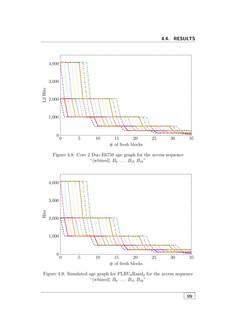
4.4. RESULTS
0 5 10 15 20 25 30 350
1,000
2,000
3,000
4,000
# of fresh blocks
L2Hits
Figure 4.8: Core 2 Duo E6750 age graph for the access sequence“〈wbinvd〉 B0 . . . B15 B10”
0 5 10 15 20 25 30 350
1,000
2,000
3,000
4,000
# of fresh blocks
Hits
Figure 4.9: Simulated age graph for PLRU8Rand2 for the access sequence“〈wbinvd〉 B0 . . . B15 B10”
99

CHAPTER 4. CHARACTERIZING CACHE ARCHITECTURES
0 5 10 15 20 25 30 35 40 450
500
1,000
1,500
2,000
2,500
3,000
3,500
4,000
4,500
# of fresh blocks
L2Hits
B0 B8 B16
B1 B9 B17
B2 B10 B18
B3 B11 B19
B4 B12 B20
B5 B13 B21
B6 B14 B22
B7 B15 B23
Figure 4.10: Core 2 Duo E8400 age graph for the access sequence“〈wbinvd〉 B0 . . . B23”
100

4.4. RESULTS
0 5 10 15 20 25 30 35 40 450
1,000
2,000
3,000
4,000
# of fresh blocks
L2Hits
Figure 4.11: Core 2 Duo E8400 age graph for the access sequence“〈wbinvd〉 B0 . . . B23 B4”
0 5 10 15 20 25 30 35 40 450
1,000
2,000
3,000
4,000
# of fresh blocks
Hits
Figure 4.12: Simulated age graph for Rand3PLRU8 for the access sequence“〈wbinvd〉 B0 . . . B23 B4”
101

CHAPTER 4. CHARACTERIZING CACHE ARCHITECTURES
B8, . . . , B15, their relative order changes in the same way as in an 8-wayset-associative cache with the PLRU policy (this corresponds to permutationΠPLRU
5 in Figure 4.2). Furthermore, we can see that the access to B10 changesthe relative order of the eight blocks B0, . . . , B7 in the same manner.
The following model agrees with these observations. Consider a PLRU-likepolicy in which the lowest bits (i.e., the bits that are closest to the leaves)are replaced by (pseudo-)randomness. In the following, we will call thispolicy PLRU8Rand2; Figure 4.5 illustrates the policy. Under this policy, oneof the two elements to which the tree bits point is replaced with a probabilityof 50%. Furthermore, after every eight subsequent misses the tree bits pointto the same subtree.
Figure 4.9 shows the result of a simulation of the PLRU8Rand2 policy onthe same access sequence that was used for Figure 4.8. We can see that thesimulation matches the actual measurements very closely.
Core 2 Duo E8400
Figure 4.10 shows an age graph for the access sequence “〈wbinvd〉 B0 . . . B23”on a Core 2 Duo E8400, which has a 24-way set-associative L2 cache. Similarlyas with the E6750, an access to Bi leads to hits in all sets if fewer than 8additional blocks have been accessed since the previous access to Bi. However,unlike with the E6750, the number of hits decreases more continuously ifmore additional blocks are accessed.
Figure 4.11 shows the effect of an additional access to block B4. This blockis now the block that gets evicted last. The relative order of the other blocksdoes not change significantly.
A possible model that leads to a similar behavior is the following. Considera PLRU-like policy in which the root node is replaced by (pseudo-)random-ness, as illustrated in Figure 4.6; in the following, we will call this policyRand3PLRU8. Under this policy, the elements are separated into three groupswith eight elements each; within each group they are managed by the PLRUpolicy. Upon a miss, one of the groups is chosen randomly.
Figure 4.12 shows the result of a simulation of the Rand3PLRU8 policy onthe same access sequence that was used for Figure 4.11. The results are quitesimilar; however, the graph of the simulation has a more regular structure. Apossible cause for the differences could be that the simulation uses a differentrandom number generator than the actual hardware.
102

4.4. RESULTS
0 20 40 60 80 100 120 140 160 180 2000
10
20
30
40
50
60
70
# of fresh blocks
L3Hits
B0 B2 B4 B6 B8 B10B1 B3 B5 B7 B9 B11
Figure 4.13: Ivy Bridge age graph for the access sequence“〈wbinvd〉 B0 . . . B11 B4”, © 2020 IEEE
0 20 40 60 80 100 120 140 160 180 2000
10
20
30
40
50
60
70
# of fresh blocks
Hits
Figure 4.14: Simulated age graph for QLRU_H11_MR161_R1_U2 for theaccess sequence “〈wbinvd〉 B0 . . . B11 B4”, © 2020 IEEE
103

CHAPTER 4. CHARACTERIZING CACHE ARCHITECTURES
4.4.3 L3 CachesThe Nehalem and Westmere CPUs use the MRU replacement policy in theirL3 caches. This was also reported by [ENBSH11]. The Sandy Bridge CPUuses a variant of this policy that, upon clearing the cache with the WBINVDinstruction, sets all status bits to one, and does not update the status bitsuntil all lines are filled.
The more recent generations use adaptive policies with different variants ofQLRU replacement.
Ivy Bridge
For the Ivy Bridge machine, we found that the cache sets 512–575 and thecache sets 768–831 (in all C-Boxes) use a fixed policy, whereas the othersets are follower sets. Figure 4.15 shows the corresponding graph that wasgenerated by the tool for analyzing adaptive policies described in Section 4.3.5.
According to our results, the sets 512–575 use the QLRU_H11_M1_R1_U2policy.
The policy used by the sets 768–831 appears to be nondeterministic. Fig-ure 4.13 shows an age graph for the access sequence “〈wbinvd〉 B0 . . . B11 B4”(note that the associativity of the cache is 12); the accesses of the sequencewere performed in all of these 64 sets.
We can see that the curves for Bi and Bi+1 (i > 0) are similar, but shifted byabout 16 (except for B4, which is accessed twice in the sequence). Furthermore,for B0, about 15
16 of the blocks are evicted immediately when the first freshblock is accessed, while the remaining 1
16 of the blocks remain in the cacherelatively long.
A policy that has a similar behavior for B0, and for which the correspondingcurves are also separated by about 16, is the QLRU_H11_MR161_R1_U2policy, i.e., a variant of the policy used in sets 512–575 that inserts new blockswith age 1 in 1
16th of the cases, and with age 3 otherwise.
Figure 4.14 shows an age graph for a simulation of this policy. The graphis similar to Figure 4.13, though not identical. One explanation for thedifferences could be that the hardware actually uses a different policy variant.However, an alternative explanation could be that the differences are due tothe hardware and the simulation using different random number generators.A more thorough investigation of the differences is left as future work.
104

4.4. RESULTS
Haswell, Broadwell
The Haswell and Broadwell CPUs use the same cache sets as the Ivy Bridgeprocessor as dedicated sets, but only in C-Box 0. All other cache sets arefollower sets.
Both CPUs use the QLRU_H11_M1_R0_U0 replacement policy in sets 512–575 in C-Box 0. The policy in sets 768–831 in C-Box 0 might be theQLRU_H11_MR161_R0_U0 policy.
Skylake, Kaby Lake, Coffee Lake, Cannon Lake
The Skylake, Kaby Lake, Coffee Lake, and Cannon Lake CPUs use theQLRU_H11_M1_R0_U0 policy in 16 fixed cache sets2. These sets were firstdiscovered by Vila et al. [VKM19, VGGK20].
Figure 4.16 shows a graph created on the Kaby Lake machine using the toolfor analyzing adaptive policies described in Section 4.3.5. This graph wascreated using cacheSeq’s option of not adding additional accesses for clearinghigher cache levels (see Section 4.3.2). The associativity of the L3 cache onthese CPUs is higher than the associativities of the higher-level caches; weverified that the sequences used for generating the graph do not lead to hitsin the higher-level caches.
The graph shows that for the 16 sets mentioned above, the test sequencesalways lead to 0 hits in the L3 cache. The policy in the remaining sets changes,depending on the number of hits and misses in the sets with the fixed policy,between this policy and a policy that is slightly more thrashing-resistant;unlike with the adaptive policies used by previous generations, there appearto be no sets that can only use the second policy.
We were not able to identify the second policy. Unlike the tool for analyzingadaptive policies, the tools for determining the replacement policy (see Sec-tion 4.3.3) require using cacheSeq’s default option that adds accesses to otherslices to clear higher-level caches on these machines. However, when usingthis option, we did not observe any differences between the two policies. Inparticular, for the thrashing sequence with (associativity+ 1) many elementsthat the tool for analyzing adaptive policies uses, we always observed 0 hitsin all sets when using this option. A further investigation of this phenomenonis left as future work.
2Sets 0, 33, 132, 165, 264, 297, 396, 429, 528, 561, 660, 693, 792, 825, 924, and 957
105

CHAPTER 4. CHARACTERIZING CACHE ARCHITECTURES
0 200 400 600 800 1,000 1,200 1,400 1,600 1,800 2,000
0
2
4
6
8
Set
L3Hits
MaxMin
Figure 4.15: Test for adaptive policies on Ivy Bridge
0 100 200 300 400 500 600 700 800 900 1,000
0
0.5
1
1.5
Set
L3Hits
MaxMin
Figure 4.16: Test for adaptive policies on Kaby Lake
106

4.4. RESULTS
0 100 200 300 400 500 600 700 800 900 1,0004
5
6
7
8
9
Set
L3Hits
MaxMin
Figure 4.17: Test for adaptive policies on Ice Lake
20 25 30 35 40 45 50 55 604
5
6
7
8
9
# accesses to other slices
L3Hits
MaxMin
Figure 4.18: Minimum and maximum number of L3 hits on Ice Lake incache set 1, depending on the number of accesses to other slices
107

CHAPTER 4. CHARACTERIZING CACHE ARCHITECTURES
Ice Lake
On Ice Lake, the same 16 cache sets described in the previous section use afixed replacement policy: they use the QLRU_H00_M1_R0_U1 policy (i.e.,the same policy as the L2 cache).
Figure 4.17 shows a graph created using the tool for analyzing adaptivepolicies described in Section 4.3.5. Unlike the graph in the previous section,this graph was created with cacheSeq’s default option that adds accesses toother slices to clear higher-level caches (this was also necessary here, as theassociativity of the L3 cache is not larger than the associativity of the L1cache).
At first sight, the graph looks similar to the graph in Figure 4.16. However,the minima and maxima of the number of L3 hits are significantly higherthan in the previous graph. Thus, the policy used in the fixed sets hassome thrashing resistance, unlike the policies in the fixed sets of previousmicroarchitecture generations. The remaining sets can switch between thispolicy and a second policy that is even more thrashing-resistant; which of thetwo policies is used depends on the recent number of hits and misses in thefixed sets.
However, further experiments showed that the exact behavior of the secondpolicy depends on the number of accesses to other slices.
Figure 4.18 shows a graph that was generated by varying the number nof accesses to other slices; the y-axis shows the number of L3 hits in cacheset 1 for the same access sequence used for generating Figure 4.17 (i.e., anaccess sequence with (associativity + 1) many elements that is repeated 10times).
For values of n such that n + 1 is a multiple of 7, the number of L3 hits isthe same for both replacement policies that set 1 can use. The tool describedin Section 4.3.3 shows that the two policies are in fact the same for thesevalues of n (for this experiment, we used special initialization sequences thatproduce a lot of hits and misses in the fixed sets, respectively, to trigger thecorresponding replacement policy in the remaining sets). For other valuesof n, the second replacement policy is none of the variants that our toolconsiders. However, the graph suggests that the second policy might be avariant of the policy used in the fixed sets that inserts new blocks with age 3instead of age 1 on every 7th access, where the corresponding access countertakes all slices into account. A further investigation of this hypothesis is leftas future work.
108

4.4. RESULTS
I0 I1 I2 I3 I4 I5 I6 I7
0 1 1 0
0 1
0
Figure 4.19: Possible PLRU state after accessing “I0 . . . I7 I1 I2 I4”
4.4.4 Resetting the Replacement Policy StateAs described in Section 4.3.3, the behavior after clearing the caches with theWBINVD instruction appeared to be nondeterministic on several microarchi-tectures. In particular, this was the case for the L1 caches of the Core 2 Duos,the Sandy Bridge, Ivy Bridge, Haswell, and Broadwell CPUs, and the L2caches of the Skylake, Kaby Lake, and Coffee Lake CPUs.
For the Sandy Bridge, Ivy Bridge, Haswell, Broadwell, Skylake, Kaby Lake,and Coffee Lake CPUs, we found out that the apparent nondeterminism isactually due to a dependency on the previous replacement policy state (i.e.,the state before the WBINVD instruction was executed). For Haswell andSkylake, this was also discovered independently by Pepe Vila [Vil19].
For the L1 caches of the Sandy Bridge, Ivy Bridge, Haswell, and BroadwellCPUs (which are 8-way set-associative and use the PLRU policy), the accesssequence
“I0 . . . I7 I1 I2 I4 〈wbinvd〉 B0 . . . B7 B8 B0?”
leads to a cache miss, whereas the sequence
“I0 . . . I7 I0 〈wbinvd〉 B0 . . . B7 B8 B0?”
leads to a cache hit.
This suggests that the PLRU tree bits are not updated when blocks areinserted into an empty cache. If blocks are inserted from left to right into anempty cache, then after executing the sequence “I0 . . . I7 I1 I2 I4”, the treebits will point to I0. This is illustrated in Figure 4.19. If the blocks after theWBINVD instruction are inserted in the same order and the tree bits are notupdated, the access to B8 will evict B0, and hence, we get a cache miss whenaccessing B0 again. On the other hand, after executing “I0 . . . I7 I0”, thetree bits will point away from I0. Thus, the access to B8 will not evict B0.
109
CHAPTER 4. CHARACTERIZING CACHE ARCHITECTURES
For the L2 caches of the Skylake, Kaby Lake, and Coffee Lake CPUs (whichare 4-way set-associative and use the QLRU_H00_M1_R2_U1 policy), theaccess sequence
“I0 I1 I2 I3 I0 I1 I2 I0 I1 I2 〈wbinvd〉 B0 B1 B2 B3 B4 B2?”
leads to a cache miss, whereas the sequence
“I0 I1 I2 I3 I0 I1 I3 I0 I1 I3 〈wbinvd〉 B0 B1 B2 B3 B4 B2?”
leads to a cache hit.
A possible explanation for this behavior is that the check whether there isstill a line with age 3 after an access uses the previous ages for lines that arecurrently empty.
We observed the same differences when using CLFLUSH instructions insteadof the WBINVD instruction.
Reset Sequences
Based on these results, we identified the following reset sequences (see Sec-tion 4.3.3) to established a fixed replacement policy state.
For the L1 caches of the CPUs mentioned above, we use the reset sequence
“I0 . . . I7”,
and for the L2 caches, we use the reset sequence
“I0 I1 I2 I3 I0 I1 I2 I0 I1 I2”.
After executing these reset sequences, the subsequent behavior was alwaysdeterministic (note that the blocks of a reset sequence are not used againlater).
Covert/Side Channels
Clearing the cache using theWBINVD or CLFLUSH instructions is sometimesrecommended as a technique for mitigating covert channels and side channels[ZBW17, GYLH16]. Ge et al. claim that after executing the WBINVDinstruction, “the caches are in a defined state” [GYLH16]. The experimentsin this section show that this is not the case for several recent processors.Using the obtained insights to implement and evaluate covert channels is leftas future work.
110

4.5. RELATED WORK
Table 4.4: Number of status bits required for different replacement policies,in terms of the associativity A.
Policy Number of Status Bits A=4 A=8 A=12 A=16 A=24
FIFO dlog2(A)e 2 3 4 4 5LRU dlog2(A!)e 5 16 29 45 80PLRU A− 1 3 7 - 15 -LRU3PLRU4 A - - 12 - 24PLRU8Rand2
A2 − 1 1 3 - 7 -
Rand3PLRU8 A− 3 - - 9 - 21MRU A 4 8 12 16 24QLRU 2 ·A 8 16 24 32 48
4.4.5 Implementation CostsThe cost of implementing a particular replacement policy can be quantifiedin terms of the minimal number of status bits that an implementation re-quires [Rei08]. Table 4.4 shows these costs for different policies, including thepolicies that we uncovered in this chapter.
4.5 Related Work
4.5.1 Microbenchmark-Based Cache AnalysisA number of papers have proposed microbenchmark-based techniques fordetermining parameters of the memory hierarchy like the cache size, the asso-ciativity, the block size, or the latency [SS95, MS96, LT98, TY00, BC00, CD01,DMM+04, Man04, JB07, YPS05, YJS+06, BT09, MHSM09, WPSAM10,GDTF+10, CS11, AR12, Abe12, DLM+13, HKP15, MC17, CX18].
While some of these approaches make assumptions as to the underlyingreplacement policy (e.g. [SS95] and [TY00] assume that LRU is used), only afew publications have also tried to determine the replacement policy.
The approaches described in [CD01] and [BC00] are able to detect LRU-basedpolicies but treat all other policies as random. John and Baumgartl’s [JB07]approach is able to distinguish between LRU and several of its derivatives.
In [Abe12, AR13], we proposed an algorithm that can automatically inferpermutation policies (see Section 4.2.2). In the present work, we developedan improved implementation of this algorithm that can infer the policies in
111

CHAPTER 4. CHARACTERIZING CACHE ARCHITECTURES
individual cache sets; the implementation in [Abe12, AR13] was based on theassumption that all cache sets use the same policy.
Henry Wong [Won13] discovered that Ivy Bridge CPUs use set dueling toswitch between two different replacement policies. He identified the sets thatuse fixed policies; however, he was not able to determine which two policiesare actually used. Similar work was described by Zhang et al. [ZGY14].
Briongos et al. [BMME19] present an approach for analyzing the replacementpolicies used by the L3 caches in recent Intel CPUs. Similar to the techniquedescribed in Section 4.3.3, their approach generates random access sequencesand compares their behavior to simulations of different policies. However,unlike in our approach, they do not measure the total number of hits thatthe sequence generates. Instead, they only determine the first element to beevicted upon the first miss after executing the access sequence. Furthermore,unlike in our approach, they rely on timing measurements instead of usingperformance counters.
Briongos et al. applied their technique to CPUs with the Haswell, Broadwell,Skylake, and Kaby Lake microarchitectures. Our results for these microarchi-tectures disagree with their results. The policies they describe would be theQLRU_H21_M2_R0_U0_UMO and QLRU_H21_M3_R0_U0_UMO variantsaccording to our naming scheme. Our tool found several counterexamplesfor these policies on all of the tested CPUs. Briongos et al. also statedthat the two policies did not agree with all of their observations; however,they assumed that “the errors were due to noise”. Furthermore, according toBriongos et al., the dedicated sets on the Haswell and Broadwell CPUs aredistributed over different slices; according to our results, they are all in thesame slice. As, according to the paper, they use an approach from [LYG+15],we assume that they also rely on a statement from that paper that “whenthe number of cores in the processor is a power of two, the set index bitsare not used for determining the LLC slice.” This was, however, shown tobe incorrect in later work [MSN+15]. Thus, their observations rather seemto be an artifact of the hash function used for determining the cache slices.Briongos et al. did not find the sets with a varying policy on Skylake andKaby Lake, and thus incorrectly concluded that these CPUs do not use anadaptive policy.
Rueda [RC13] developed a technique for learning replacement policies usingregister automata. He was able to learn the FIFO and LRU policies for cacheswith an associativity of at most 5, and the PLRU and MRU policies for cacheswith an associativity of at most 4. He did not successfully apply his techniqueto actual hardware.
112
4.5. RELATED WORK
In concurrent work, Vila et al. [VGGK20] describe an approach for inferringreplacement policies using automata learning, and an approach for automati-cally generating human-readable representations of the learned policies. Forsoftware-simulated caches, they were able to learn FIFO and PLRU up toassociativity 16, MRU up to associativity 12, and several other policies upto associativity 6. Furthermore, Vila et al. also applied their techniques toactual hardware with the Haswell, Skylake, and Kaby Lake microarchitectures.They successfully learned the policies used by the L1 and L2 caches of thesethree processors, as well as the policy used by the leader sets of the L3 cacheson Skylake and Kaby Lake. Their results agree with our results. Vila et al.’sapproach was, however, not able to learn the policies used by the L3 cache ofthe Haswell CPU, as the associativity was too high for their approach, andone of the policies is nondeterministic.
Vila et al.’s approach relies on a tool called CacheQuery, that is quite similarto the CacheSeq tool proposed in Section 4.3.2. The main differences are thefollowing:
1. CacheQuery uses a more expressive syntax,
2. CacheQuery is based on timing measurements, whereas CacheSeq usesperformance counters, and
3. CacheQuery requires the parameters of the caches, such as the associa-tivities or the number of cache sets, to be specified manually, whereasCacheSeq determines them automatically using CacheInfo.
4.5.2 Influence of the Replacement Policy on Perfor-mance Prediction Accuracy
Multiple works have identified the cache replacement policy as an importantfactor for the accuracy of performance prediction techniques.
Grund et al. [GR08] describe an analytical method to estimate miss ratiosfor a given cache configuration. They consider the replacement policy tobe an important component that “can have a significant influence on thecache performance.” Guo et al. [GS06] present an analytical model for cachereplacement policy performance and claim that the “replacement policy is afactor that should be taken into account in designing a cache and modelingcache performance.” Tam et al. [TASS09] model the performance of a systemin terms of miss rate curves (MRCs) that plot the miss rate of an accesssequence as a function of the cache size. They state that “the MRC of aLeast Recently Used (LRU) policy may be significantly different from that of
113

CHAPTER 4. CHARACTERIZING CACHE ARCHITECTURES
a Most Recently Used (MRU) policy for the same memory access sequence.”Furthermore, according to Kegley et al. [KPD+11], the replacement policy“can substantially influence the performance of a system.”
Unfortunately, current performance modeling approaches often do not considerdifferent policies. Tam et al.’s approach [TASS09], for instance, only supportsLRU as they believe that “it is the most commonly used replacement policy.”Similarly, Fraguela et al. [FDTZ04] claim that LRU “nowadays is by far themost common” policy. As our work shows, this is not true for most currentmicroarchitectures.
4.5.3 Security Aspects of Replacement PoliciesCaches are at the center of many covert-channel and side-channel attacks[OST06, GBK11, YF14, LYG+15, GMWM16, DKPT17, MWK17, TLM18,GYCH18, DXS19, vSMK+20, LHS+20].
Several papers show that knowledge of the replacement policy can be impor-tant for devising or mitigating such attacks.
In [KMO12], Köpf et al. propose a technique for automatically derivingupper bounds on the amount of information leakage through cache sidechannels. They focus on the LRU replacement policy. CacheAudit [DKMR15,BKMO14, DK17, CnKR17] improves upon this work by considering moretypes of adversaries, by providing tighter bounds, and by considering differentreplacement policies. In particular, their current implementation supportscaches that use the FIFO, LRU, and PLRU policies.
In [CnKR19], Cañones et al. present techniques for comparing caches withdifferent replacement policies with respect to their vulnerability to side-channelattacks.
Accessing memory locations with a high frequency can lead to bit flips inneighboring DRAM rows [KDK+14]; this phenomenon is commonly called theRowhammer bug. Gruss et al. [GMM16] describe a JavaScript-based attackthat exploits this bug to obtain unrestricted access to the systems of websitevisitors. To this end, they require an efficient eviction strategy, i.e., an accesssequence that can be used instead of the CLFLUSH instruction, which isnot available in JavaScript. Whether an eviction strategy is efficient on aspecific CPU depends on the replacement policy. As Gruss et al. do not knowthe replacement policies used in recent Intel CPUs, they go to great lengthsto find suitable eviction strategies; overall, they evaluate more than 18, 000possible strategies.
114

4.6. CONCLUSIONS AND FUTURE WORK
Kim et al. describe StealthMem [KPMR12], a technique that manages aset of locked lines which are never evicted from the last-level cache. Theirimplementation is based on the assumption that the cache has the k-LRUproperty, which means that the replacement policy will never evict the kmost-recently accessed blocks. To find a value for k for which their pro-cessor with the Nehalem microarchitecture has the k-LRU property, theypropose the following experiment. They use access sequences of the form“B0 B1 . . . Bk′ B0?” and evaluate them with increasing values for k′ between1 and 16 (which corresponds to the associativity). They start seeing L3misses at k′ = 15 and conclude that the cache has the 14-LRU property.This is incorrect. According to the results in this chapter, and also accord-ing to Eklov et al. [ENBSH11], the L3 caches of Nehalem-based processorsuse the MRU replacement policy. Caches with this policy do not have thek-LRU property for any k > 1. As an example, consider the access sequence“〈wbinvd〉 B0 . . . B14 B0 B15 B16 B0?”. The access to B15 will flip the statusbits of all other blocks. Consequently, the access to B16 will evict B0, andthus, the final access to B0 will lead to a cache miss. We verified that this isindeed the case on our Nehalem system.
Kiriansky et al. [KLA+18] propose hardware modifications to defend againstcache timing attacks. In particular, they propose a cache partitioning tech-nique that, unlike previous partitioning techniques, takes the state of thereplacement policy into account to ensure isolation. They describe implemen-tations of this technique for PLRU, MRU, and SRRIP.
Briongos et al. [BMME19] present an attack that exploits the state of theL3 replacement policy to extract information from a victim; their attackis undetectable by countermeasures that rely on monitoring cache misses.Xiong and Szefer [XS20] describe a related attack that uses the state of thereplacement policy in the L1 cache to leak information.
4.6 Conclusions and Future WorkWe developed several tools that generate microbenchmarks for analyzingproperties of caches, focusing, in particular, on cache replacement policies.We applied our tools to 13 recent Intel microarchitectures, and we identifiedseveral previously undocumented replacement policies. Furthermore, wediscovered that, contrary to popular belief, flushing the cache does notnecessarily reset the state of the replacement policy; this might be used todevise new covert-channel and side-channel attacks.
115

CHAPTER 4. CHARACTERIZING CACHE ARCHITECTURES
Future Work
There are multiple directions for future work. One goal is to increase the classof policies that can be inferred fully automatically. Currently, our tools are ableto infer all permutation policies, as well as around 300 deterministic policiesthat are not permutation policies. A promising approach is to use automatalearning techniques, as shown by Rueda [RC13] and Vila et al. [VGGK20].Future work would include enhancing these approaches to support largerassociativities. Furthermore, it would be interesting to develop techniquesthat can identify nondeterministic policies automatically.
Another direction for future work would be to add support for non-IntelCPUs. For AMD CPUs, it would likely be sufficient to make our algorithmsrobust against noise introduced by the prefetchers, which cannot be disabledon these CPUs. A related goal would be to infer models of the prefetchersthemselves. To add support for non-x86 CPUs, we would need to extendnanoBench, as proposed in Section 2.6.
Furthermore, we would like to extend our tools to also support instructionand µop caches (see Section 3.3), which are typically only poorly documented.
116

5Gray-Box Learning of Serial
Compositions of Mealy Machines
The techniques we proposed in the previous chapters can be seen as instancesof active learning approaches. Active learning (also called query learning)refers to a class of machine-learning techniques in which the learning algorithmis able to interact with the system to be learned.
The techniques described in the previous chapters were heavily targeted at thespecific problems. In this chapter, we look at more general techniques. Specif-ically, we consider approaches for learning finite state machines, which are, inprinciple, suitable abstractions for modeling the behavior of microarchitecturalcomponents.
Most existing learning algorithms for finite state machines treat the systemto be learned as a black box. These algorithms often do not scale to complexrealistic systems, as the state space of such systems is typically too large.
In this chapter, we propose the concept of gray-box learning for dealing withsuch systems. The main idea hereby is to use available information about thesystem to focus the learning algorithms on the parts that are unknown.
As a first step toward solving this problem, we study one specific instance.We consider the serial composition of two Mealy machines A and B, whereA is known and B is unknown, and we assume that we can only performqueries on the composed machine. For this scenario, we develop an efficientalgorithm that learns a model of the unknown machine B.
This chapter is an extended version of [AR16]. We provide more details onthe SAT reduction (in Section 5.5.1), and proofs for the lemmas and theorems(in Appendix 5.A), which were omitted from the original publication due tospace reasons.
117

CHAPTER 5. GRAY-BOX LEARNING
5.1 IntroductionTools to analyze software or hardware systems, such as static analyzers ormodel checkers, require accurate models as input. Third-party components,however, are rarely specified at the level of detail required by such tools.
One approach to automatically obtain formal models of systems is activelearning [Set11]. Here, one commonly assumes an oracle, or teacher, thatadmits two kinds of queries about the system: output queries return the resultof the system for a specific input, and equivalence queries check whether aconjectured model is consistent with the system to be learned and return acounterexample if not. Based on this setup, Angluin introduced the L∗ al-gorithm [Ang87] for learning deterministic finite automata. L∗ has sincebeen extended to other modeling formalisms, such as Mealy machines [SG09],register automata [HSJC12, BHLM13, AFBKV15], or symbolic automata[MM14]. It is also at the heart of several model checking approaches, includ-ing [CGP03, GPY02, VSVA05].
As the system is treated as a black box, no information about the internalstructure of the system can be taken into account by most existing learningalgorithms. In practice, however, systems are often composed of subcompo-nents, for some of which models might be available, but it is not possibleto access the known and the unknown parts separately from the outside.Partial information about the inner workings of a system may be inferredfrom manuals or conjectured from similar, yet better documented systems.This scenario is depicted in Figure 5.1.
While it is in theory possible to learn a model of the entire system usingexisting black-box approaches, this is often not viable in practice because thestate space is too large. A problem, which has received little attention in theliterature so far, is how to use the available information about the system tofocus the learning algorithm on those parts that are unknown. This problemcould be termed gray-box learning.
In this chapter, as a first step toward solving this problem, we study onespecific instance: We assume that the system C is the serial composition oftwo Mealy machines A and B, and that we have a model for the left machine(A) and want to learn the right machine (B). We further assume that we canperform output and equivalence queries only on C as a whole. This scenariois shown in Figure 5.2.
While output queries can often be realized cheaply by measurements on theactual system, equivalence queries can usually only be approximated by a
118

5.2. PROBLEM STATEMENT
I O
Figure 5.1: Mealy machine network
A BOA IBI O
C
Figure 5.2: Serial composition
large number of such measurements. Our primary focus is thus to minimizethe number of equivalence queries. We introduce an algorithm to exactlylearn B in the context of A that performs at most |B| equivalence queries,where |B| denotes the number of states of B.
We evaluate our approach on compositions of randomly-generated machinesagainst an implementation of the classic L∗ algorithm in LearnLib [IHS15].We show that our approach requires significantly fewer output and equivalencequeries on most benchmarks.
5.2 Problem StatementIn this section, we first formally define several concepts used throughout thischapter. Then, we give a precise description of the problem that we address.
5.2.1 Basic NotionsDefinition 5.1 (Completely Specified Mealy Machine). A completely speci-fied Mealy machine is a tuple (Q, I,O, δ, qr), where
• Q 6= ∅ is a finite set of states
• I 6= ∅ is a finite set of input symbols
• O 6= ∅ is a finite set of output symbols
• δ : Q× I → Q×O is the transition function
• qr ∈ Q is the initial (reset) state.
In this chapter, we only consider completely specified Mealy machines; incom-pletely specified Mealy machines are introduced in Chapter 6.
119

CHAPTER 5. GRAY-BOX LEARNING
We extend δ to sequences in the usual way. We use ε to denote the emptysequence. Further, we use M(x) to denote the output sequence of a Mealymachine M when reading x, and ML(x) to denote the last output of M whenreading x.
Given two Mealy machines A and B, we can compose them to a serial Mealymachine C by using the output of A as the input for B. Formally:
Definition 5.2 ((Synchronous) Serial Composition of Mealy Machines).Let A = (QA, IA, OA, δA, qr,A) and B = (QB, IB, OB, δB, qr,B) be two Mealymachines such that OA ⊆ IB. The serial composition of A and B is a Mealymachine C = (Q, I,O, δ, qr), where
• Q := QA ×QB
• I := IA
• O := OB
• δ((qA, q
B), i) := ((q′
A, q′
B), o), where (q′
A, o
A) := δA(q
A, i), and (q′
B, o) :=
δB(qB, o
A)
• qr := (qr,A , qr,B )
Given a composition of two Mealy machines A and B, we define a machine B′to be right-equivalent to B in the context of A if the composition of A and Bdescribes a machine that is equivalent to the composition of A and B′.Formally:
Definition 5.3 (Right-Equivalence). Let A,B, and B′ be Mealy machines.Then, B′ is right-equivalent to B in the context of A iff
∀x ∈ I∗ : B(A(x)) = B′(A(x)).
5.2.2 The Gray-Box Learning ProblemIn this chapter, we address the following problem. We assume that we have aserial composition C of two Mealy machines A and B. Further, we assumethat we have a model of A, but B is unknown. While we do not have a modelof C, we assume that we can determine the output of C on any input by anoutput query, and we can test whether a machine is equivalent to C by anequivalence query.
Using existing techniques, like Angluin’s L∗ algorithm [Ang87], one couldconsider C to be a black box and learn a model of C. Such an approach would
120

5.3. PRELIMINARIES
in the worst case employ a polynomial number of output and equivalencequeries in the size of C, which can be up to |A| · |B|.
Instead, our goal is to exploit the knowledge we have about A, and to learn amodel of a minimum-size machine B′, such that B′ is right-equivalent to B inthe context of A. In particular, as we consider equivalence queries to be moreexpensive than output queries, we want the number of equivalence queries tobe polynomial in the number of states of B′, independently of the size of A.
5.3 PreliminariesExisting active learning approaches for Mealy machines (and related machinetypes) are usually based on a Myhill-Nerode-like equivalence relation thatpartitions the set of input words into classes such that the words that are inthe same class cannot be distinguished with respect to different suffixes:
Definition 5.4 (Equivalence of Input Words). Given a function F : I∗ → O,two words x, y ∈ I∗ are equivalent, x ∼ y, iff
∀z ∈ I∗ : F (x · z) = F (y · z).
F can be modeled by a Mealy machine iff this relation has finitely manyequivalence classes. One can then construct a minimum-size Mealy machinewhose states are the equivalence classes of this relation. Existing approachescompute the equivalence relation in a co-inductive fashion. In the beginning,they consider all words to be equivalent. Then, in each round, this hypothesisis refined by identifying at least one new equivalence class, until the equivalencerelation is fully determined.
If we consider the machine B in the serial composition with A, then it ispossible that not all input sequences for B can be produced by A. Lettr(A) = {A(x) | x ∈ I∗} be the set of output sequences that A can produce.For each output sequence x ∈ tr(A), there might be multiple input sequencesthat produce this output. Let A−1 : tr(A) → I∗ be a function such thatA−1(x) returns one of these input sequences. In the following, it will not beimportant which of the possibly multiple sequences is actually returned.
We have that every right-equivalent Mealy machine B′ for B in the contextof A has to agree with the partial function FP : I∗B ⇀ O such that
∀x ∈ tr(A) : FP (x) = BL(x).
Note that while we do not have immediate access to B, we can use outputqueries on C to access B, as for all x ∈ tr(A), BL(x) = CL(A−1(x)).
121

CHAPTER 5. GRAY-BOX LEARNING
Similarly to Definition 5.4, we define two words to be right-compatible in thecontext of A iff they cannot be distinguished with respect to different suffixes.
Definition 5.5 (Right-Compatibility). Two words x, y ∈ I∗B are right-com-patible in the context of A, x ∼A y, iff
∀z ∈ I∗B : (xz /∈ tr(A) ∨ yz /∈ tr(A) ∨BL(xz) = BL(yz)).
Otherwise, x and y are incompatible, x �A y.
However, right-compatibility is, unlike equivalence, not transitive. Thus,it is not an equivalence relation, which means we cannot directly use theconstruction sketched above to build a minimum-size machine.
To see this, consider three output symbols a, b, c ∈ OA with
∀z ∈ I∗B : az, bz ∈ tr(A) ∧BL(az) = 0 ∧BL(bz) = 1
and∀z ∈ I∗B : cz /∈ tr(A).
So B always outputs 0 if the first output of A was a, it always outputs 1 ifthe first output of A was b, and A never outputs c as the first output.
This means that a ∼A c and b ∼A c, but a �A b. For this example, we canbuild a machine with three states that is right-equivalent to B. From thestart state, a transition with c can go to any state. This also shows thatthere can be multiple machines with the minimum number of states that areright-equivalent to B.
5.4 ApproachEquivalence queries are typically assumed to be more expensive than outputqueries. Many existing active learning techniques therefore focus on keepingthe number of required equivalence queries low.
At a high level, Angluin’s L∗ algorithm for instance, can be described asfollows. In each round, the algorithm first performs a sequence of outputqueries in a systematic way, until there is exactly one machine of minimumsize that is consistent with the results from all output queries performed sofar. Only then, the algorithm performs an equivalence query. If this queryreturns a counterexample, this implies that the correct machine must haveat least one additional state. Thus, Angluin’s algorithm performs at most nequivalence queries, where n is the size of the minimal correct machine.
122

5.4. APPROACH
Unlike in Angluin’s setting, in general no unique machine of minimum sizethat is consistent with a set of observations exists. The basic idea behindour approach is to perform output queries until all machines of minimumsize that are consistent with these queries are right-equivalent in the contextof A. We then perform an equivalence query for one of these machines. Ifthis query results in a counterexample, this counterexample witnesses thatall of these machines are incorrect, and thus, the correct machine must haveat least one additional state.
One challenge is to find a suitable sequence of output queries that is guaran-teed to reduce the number of machines that are consistent with all queriesperformed so far. The basic idea is to iteratively construct all machines ofminimum size that agree with all of the previous queries. We can then checkwhether each pair of these machines is right-equivalent. If they are not, weuse a distinguishing sequence as a counterexample, without performing anequivalence query.
However, applying this approach naively would not be viable in many casesbecause there can be an exponential number of machines of the same size thatare consistent with a set of observations, in particular in the beginning, whenonly a small number of queries have been performed. Thus, we identify anumber of necessary conditions for candidate machines to be right-equivalentwhich can be efficiently determined on observation tables. Some of theseconditions correspond to notions from Angluin’s algorithm, such as consistencyand closedness, while others, like input-completeness, are special to ourparticular setting.
In the rest of this section, we describe our proposed algorithm in detail andintroduce the necessary theoretical concepts. In particular, we describe indetail which output queries our algorithm performs to systematically reducethe number of machines that are consistent with the observations made so far.
5.4.1 Observation TablesThe main data structure used in our approach is an observation table. Therows of the table are indexed by a set of prefixes, the columns by a set ofsuffixes, and the entries of the table store the last output symbol of an outputquery for the concatenation of the corresponding prefix and suffix. If thisconcatenation is not a possible output sequence of the left machine A, wedo not perform an output query but store ⊥ in this cell instead. In contrastto most previous definitions, our observation tables do not consist of twoexplicitly distinguished parts.
123

CHAPTER 5. GRAY-BOX LEARNING
Definition 5.6 (Observation Table). An observation table T = (S,E,Q)consists of
• a finite non-empty prefix-closed set of prefixes S ⊆ tr(A)
• a finite suffix-closed set of suffixes E ⊆ I∗B (such that IB ⊆ E, andε /∈ E)
• a function Q : (S,E) → OB such that Q(x, e) = CL(A−1(xe)) iffxe ∈ tr(A) and Q(x, e) = ⊥ otherwise.
For a set R ⊆ S and a ∈ IB, let SuccT (R, a) := {xa | x ∈ R ∧ xa ∈ S}, i.e.,SuccT (R, a) is the set of successor rows for elements of R that are in thetable.
In the following, we will use the term row both for the prefixes and for theentries of a row, when it is clear what is meant from the context.
We call two rows compatible if all columns that are not ⊥ are the same inboth rows.
Definition 5.7 (Compatibility). The rows for two prefixes x, y ∈ S arecompatible iff ∀e ∈ E : Q(x, e) = ⊥ ∨Q(y, e) = ⊥ ∨Q(x, e) = Q(y, e).
We call an observation table consistent if whenever two rows are compatible,their successors are also compatible.
Definition 5.8 (Consistency). An observation table T is consistent iff for allprefixes x, y ∈ S such that the rows for x and y are compatible, for all a ∈ IBall rows in SuccT ({x, y}, a) are compatible.
If there is a suffix e ∈ E that shows that the successors of x and y under aninput a are not compatible, then ae is a suffix that shows that the rows forx and y are also not compatible. Thus, we can add ae to E to resolve thisinconsistency.
We define a partition of the set of rows as follows.
Definition 5.9 (Partition). A partition for an observation table T=(S,E,Q)is a partition P = {P1, ..., Pk} of S, such that
• for all x, y ∈ Pi: the rows for x and y are compatible,
• for each Pi and for all a ∈ IB, there is a Pj such that SuccT (Pi, a) ⊆ Pj .
Note that if SuccT (Pi, a) 6= ∅, then there is only one such Pj since all classesof the partition are disjoint.
124

5.4. APPROACH
We will later show how we can use partitions to build candidate machines thatare consistent with the observations made so far. The words in the same classof a partition will then lead to the same states in these candidate machines.
We call a partition closed if for each class of the partition and each inputsymbol a, the observation table contains a successor row (under a) for at leastone word of this class, if we know from the observations made so far thatsuch a successor must exist. Our inference algorithm uses closedness as a wayto determine which additional rows should be added to the table.
Definition 5.10 (Closedness for Partitions). Let P = {P1, ..., Pk} be apartition for T = (S,E,Q). P is closed if for all Pi ∈ P : if there is somex ∈ Pi and some sequence az ∈ E with a ∈ IB and z ∈ I∗B such thatQ(x, az) 6= ⊥, then there must be some y ∈ Pi for which Q(y, az) 6= ⊥, andya ∈ S.
Given an observation table T , let Π(T, n) be the set of all partitions of size n.Let Πmin(T ) be the set of partitions of minimum size for an observationtable T , i.e., Πmin(T ) = Π(T,m) where m = min{n | Π(T, n) 6= ∅}.
Definition 5.11 (Closedness). An observation table T = (S,E,Q) is closedif all minimum-size partitions P ∈ Πmin(T ) are closed.
Definition 5.12 (Partial Closedness). An observation table T is partiallyclosed (p-closed) iff for all prefixes x ∈ S and all sequences az ∈ E such thatQ(x, az) 6= ⊥, there is a prefix y ∈ S such that the rows for x and y arecompatible, Q(y, az) 6= ⊥ and ya ∈ S.
If a table is not p-closed, then no partition can be closed.
Definition 5.13 (Agreement). A Mealy machine M agrees with an observa-tion table T = (S,E,Q) if for all x ∈ S and e ∈ E, Q(x, e) = ⊥ ∨Q(x, e) =ML(xe).
For any closed partition P = {P1, ..., Pk} in Πmin(T ), we can build thefollowing Mealy machine MP = (Q, I,O, δ, qr) with k + 1 states:
• Q := P ∪ {error}
• I := IB
• O := OB ∪ ⊥
• δ(Pi, a) := (error,⊥) if SuccT (Pi, a) = ∅, otherwise: δ(Pi, a) := (Pj, b)such that for some x ∈ Pi: Q(x, a) = b 6= ⊥ and SuccT (Pi, a) ⊆ Pj
• qr := Pi such that ε ∈ Pi
125

CHAPTER 5. GRAY-BOX LEARNING
This machine enters a special error state if there is a class of the partition forwhich the successor class is not defined.
In the following, we will use the notation πi(t) to denote the i-th componentof a tuple t, e.g., π2(qr, a) = a.
Lemma 5.1. Let P be a closed partition of an observation table T=(S,E,Q),and let MP = (Q, I,O, δ, qr) be the Mealy machine constructed as describedabove. Then for all words x ∈ S, x ∈ π1(δ∗(qr, x)).
Theorem 5.1. For a closed partition P of an observation table T , the machineMP agrees with T .
Definition 5.14. Let γ(MP ) be the set of machines with k states that can beobtained from MP by removing the error state and replacing the transitionsto the error state by transitions with arbitrary outputs and successor states.
Theorem 5.2. Let T be a closed observation table. Then every minimum-sizemachine M that agrees with T is isomorphic to an element of γ(MP ) forsome P ∈ Πmin(T ).
Theorem 5.3. If for a closed partition P the error state is not reachable in acomposition of A with MP , then all machines in γ(MP ) are right-equivalent.
If the error state is reachable, we can use an input sequence that leads to theerror state to extend the observation table.
Definition 5.15 (Input-Completeness). An observation table T = (S,E,Q)is input-complete if for all minimum-size partitions P ∈ Πmin(T ), the errorstate is not reachable in a composition of A with MP .
Definition 5.16 (Uniqueness). An observation table T = (S,E,Q) is uniqueif for all pairs of minimum-size partitions P, P ′ ∈ Πmin(T ), the machines MP
and MP ′ are right-equivalent in the context of A.
It follows that all machines of minimum-size size that agree with a consistent,closed, input-complete, and unique observation table are right-equivalent, andthey can be obtained from the partitions.
5.4.2 Inference AlgorithmAt a high level, our algorithm works as shown in Algorithm 5.1. In eachiteration of the main loop, we first make sure that the observation table isconsistent and p-closed (by adding additional rows and columns if necessary).Then, we successively determine the partitions of minimum size for theobservation table. Whenever we find a partition that is not closed, we add
126

5.4. APPROACH
Algorithm 5.1: Main algorithmInput: Machine A, OutputQuery OQ, EquivalenceQuery EQ
1 begin2 ObservationTable OT ← empty table3 addRow( [ε])4 curSize ← 15 while true do6 while ¬consistent ∨ ¬p-closed do7 makeConsistent() // consistency8 makePClosed() // p-closedness
9 partitions ← ∅10 prevMachine ← ⊥11 while true do12 partition ← findNextPartition(partitions, curSize)13 if partition = ⊥ then14 if prevMachine = ⊥ then15 curSize ← curSize + 116 continue17 else18 counterexample ← EQ(prevMachine)19 if counterexample = ⊥ then20 removeErrorState(prevMachine)21 return prevMachine22 else23 handleCounterexample(counterexample)24 break
25 if ¬isClosed(partition) then26 closePartition() // closedness27 break28 machine ← getMachineForPartition(partition)29 errorPath ← getPathToErrorStateInComposition(A,machine)30 if errorPath 6= ⊥ then31 handleCounterexample(errorPath) // input-completeness32 break33 if prevMachine 6= ⊥ then34 distInput ← checkRightEquivalence(A, machine, prevMachine)35 if distInput 6= ⊥ then36 handleCounterexample(distInput) // uniqueness37 break
38 partitions ← partitions ∪ {partition}39 prevMachine ← machine
127
CHAPTER 5. GRAY-BOX LEARNING
new rows to the table such that the partition becomes closed, and we continuewith the next iteration of the main loop. If we find a closed partition, we checkwhether the error state is reachable in a composition of the correspondingmachine with A. If we find a sequence that leads to the error state, this meansthat the table is not input-complete. Thus, we add this sequence (and itsprefixes) to the observation table and continue with the next iteration of themain loop. If we find more than one closed and input-complete partition in thesame iteration of the main loop, we check whether the machines for these twopartitions are right-equivalent in the context of A. If we find a distinguishingsequence, we extend the observation table accordingly, and continue withthe next iteration of the main loop. If finally the table is consistent, closed,input-complete, and unique, we perform an equivalence query for the lastmachine we found (which is right-equivalent to all machines of minimum sizethat agree with the table). If the equivalence query is successful, we are done,otherwise, we get a counterexample that we add to the table.
5.5 ImplementationIn this section, we describe how our algorithm can be implemented. We alsopropose some improvements that make the algorithm more usable in practice.
5.5.1 Computing the PartitionsWe reduce the problem of finding the partitions for a given size n to a Booleansatisfiability (SAT) problem. A related reduction was used by Heule andVerwer [HV10] for finding DFAs that agree with a set of positive and negativeinput samples. However, in contrast to our approach, their approach directlycomputes one arbitrary machine that agrees with the samples. On the otherhand, our approach computes a partition which, in general, corresponds to amachine, in which some transitions may be unspecified (if the partition is notclosed or input-complete). Thus, we can exploit this additional informationto determine which output queries should be performed.
SAT solvers typically require the problem to be in conjunctive normal form(CNF). We first give a high-level description of each subproblem, and thenshow how to translate it to CNF.
In the following, we will use literals of the form rx,i ∈ B to denote that row xis in class i of the partition. We assume that the rows are numbered from 0to |S| − 1.
128

5.5. IMPLEMENTATION
Covering Condition
All rows of the table must be in at least one class. We therefore add, for allrows x, a clause of the form
rx,0 ∨ rx,1 ∨ · · · ∨ rx,n−1.
Disjointness
No row must be in more than one class. This can be expressed by adding, forall rows x and classes i, the following implication:
rx,i =⇒∧j>i
¬rx,j
In CNF, this corresponds to the following set of clauses:∧j>i
(¬rx,i ∨ ¬rx,j)
Compatibility
All rows that are in the same class must be pairwise compatible. For a row x,let Inc(x) be the set of rows that are incompatible to x. To ensure that noincompatible rows are in the same class, we add for each row x and eachclass i the implication
rx,i =⇒∧
y∈Inc(x)y>x
¬ry,i.
In CNF, this corresponds to ∧y∈Inc(x)y>x
(¬rx,i ∨ ¬ry,i).
Common Successors
For all rows that are in the same class i and for which the observation tablealso contains their successor rows for a given input a, there must be a class jthat contains all these successor rows. Thus, we have for each input symbola and each class i a clause of the form
∃j : ∀x : (rx,i =⇒ rx′,j),
where x′ is used to denote the successor row of x under input a. If theobservation table does not contain this successor row, the correspondingimplication is omitted.
129

CHAPTER 5. GRAY-BOX LEARNING
In the above formula, we can represent the existential quantifier as a dis-junction, and the universal quantifier as a conjunction. The formula is thusequivalent to ∨
0≤j<n(∧x
(¬rx,i ∨ rx′,j)).
A direct conversion of this formula to CNF would lead to an exponentialincrease in its size. To obtain a more compact representation, we introducean auxiliary literal for each input symbol and class of the form Za,i
j . Thefollowing formula is then equisatisfiable to the formula above:
(∨
0≤j<nZa,ij ) ∧
∧0≤j<n
∧x
(¬Za,ij ∨ ¬rx,i ∨ rx′,j)
Finding a Partial Solution
Since we are only interested in sets of classes, the ordering of the classes doesnot matter. Thus, by assigning some rows to a fixed class, we can significantlyreduce the number of symmetrical cases the SAT solver has to consider.We exploit this by precomputing a “partial solution”. More specifically, wefirst compute a set R = {x0, . . . , xk} of pairwise incompatible rows. For allsolutions of the SAT problem, each of these rows must be in a separate class.Thus, we can obtain an equisatisfiable formula by just assigning all elementsof R to arbitrary, different classes. To this end, we replace the covering clausesof the rows in R by the clause
rx0,0 ∧ rx1,1 ∧ · · · ∧ rxk,k.
Furthermore, for a row xi ∈ R, we can remove all literals rxi,j such that j 6= ifrom the SAT formulation and simplify the other constraints accordingly.
Moreover, we can also use the cardinality of R as a lower bound for therequired number of classes.
If we represent the compatibility relation on the rows as a graph (such thatthere is an edge whenever two rows are compatible), the problem of findingsuch a set R corresponds to finding an independent set in the graph. Whilethe problem of finding a maximum independent set is NP-hard, a heuristicis sufficient for our purposes, since a non-maximal set would just lead to asmaller reduction of symmetries, and to a smaller lower bound, but it wouldstill lead to a correct solution.
We use the following simple sequential greedy heuristic to find a set of pairwiseincompatible rows. We first create a list of all rows that is sorted in reverse
130

5.5. IMPLEMENTATION
order based on the number of incompatible rows for each row. The algorithmmaintains a set R of pairwise incompatible rows, where R is initially empty.We then iterate over the sorted list of rows. Whenever we encounter a row thatis incompatible to all rows in R, we add this row to R. A similar approachwas used by [HV10].
Excluding Previously Discovered Partitions
Since our algorithm searches for multiple partitions for the same observationtable, we add for each previously found partition a disjunction of the negatedliterals for this partition.
5.5.2 Reachability of the Error StateIf the error state is reachable with an input a from a state in the compositionof the hypothesis machine with the left machine A, this means for no prefix pin the observation table that leads to this state, the input pa is a possibleoutput of the left machine, however, there is another possible output sequencethat leads to the same state that has a corresponding successor. We can thususe this sequence as a counterexample.
A straightforward way to check the reachability would be to build the com-position, and then to perform a breadth-first search on the composition. Anecessary condition for the reachability of the error state in the composition isthat the error state is reachable in the hypothesis machine. We have observedthat in practice, if the error state is reachable in the hypothesis machine,then in many cases, it is also reachable in the composition. Thus, we usethe following approach to find a corresponding sequence quickly: We firstdetermine for each state of the hypothesis machine the distance of the shortestpath to the error state. We then use this distance to guide the search in amodified breadth-first search in the composed machine.
5.5.3 Checking if Two Machines are Right-EquivalentA straightforward way to check whether two hypothesis machines B and B′are equivalent in the context of A would be to compose both with A, and thencheck the two compositions for equivalence, for example using Hopcroft-Karp’snear-linear algorithm. However, this can be computationally expensive whenA is large compared to B and B′, as it requires building the compositiontwice.
131

CHAPTER 5. GRAY-BOX LEARNING
Therefore, we take the following alternative approach. We build a newmachine D that outputs 1 iff the outputs of B and B′ differ on (a prefixof) the corresponding input, and 0 otherwise. While the size of D can bequadratic in the size of B, we have observed that, after minimization, inpractice the sizes are smaller or comparable to B. To check whether B andB′ are right-equivalent we can then just check whether the composition of Awith the minimized version of D can output 1, using the search algorithmdescribed in the previous section.
5.5.4 Handling CounterexamplesLike in the original version of Angluin’s L∗ algorithm, we handle counterex-amples by adding all prefixes of the counterexamples as rows to the table.Since, in general, the length of a counterexample can depend on |C|, thenumber of rows that are added (and hence the number of output queries thatneed to be performed to determine their entries) is not independent of |A|.
Rivest and Schapire [RS93] described an improved approach to handle coun-terexamples that needs to perform only a logarithmic number of membershipqueries (in the length of the counterexample). However, it is not possibleto directly adapt this method to our setting, since it requires that there isalways a suffix of the counterexample that is a distinguishing suffix for twocompatible rows. It is future work to develop more advanced methods to dealwith counterexamples in our setting.
5.6 EvaluationIn this section, we compare two variants of our approach with the Mealymachine version of Angluin’s L∗ algorithm. We use a set of randomly generatedcompositional Mealy machines with between 1,000 and 1,000,000 states, andan input and output alphabet of size 4.
The results are shown in Figure 5.3. GBLearning (“Gray-box Learning”)is an implementation of the approach described in the previous sections.GBLearning-Simple is a variant of our approach that does neither checkwhether the error state is reachable, nor whether different machines thatare consistent with the observation table are right-equivalent. Instead, itimmediately performs an equivalence query upon finding a closed partition.Thus, the number of equivalence queries of this variant is not independent ofthe size of the right machine.
132

5.6. EVALUATION
GBLearning GBLearning-Simple LearnLib/Comp LearnLib/⊥
(1000;1)
(100;10)
(10;100)
(1;1000)
(10000;1)
(1000;10)
(100;100)
(10;1000)
(1;10000)
(100000;1)
(10000;10)
(1000;100)
(100;1000)
(10;10000)
(1;100000)
(1000000;1)
(100000;10)
(10000;100)
(1000;1000)
(100;10000)
(10;100000)
(1;1000000)
100
102
104
106
#O
Q
1248
1632
#E
Q
0.1
1
10
100
Tim
e/s
05
10
TO
+E
Figure 5.3: Evaluation on randomly-generated machines
We compare these implementations with two variants of Angluin’s L∗ algo-rithm, as implemented in LearnLib [IHS15] (ExtensibleLStarMealy). Learn-Lib/Comp treats the system as a black box and learns the composition.Furthermore, we modified LearnLib (LearnLib/⊥) such that it uses L∗ on theright machine; impossible inputs are assumed to result in a special outputsymbol (⊥). Equivalence queries are performed by first composing the hy-pothesis for the right machine with the left machine. Note that this variantdoes not learn a minimum-size machine; in fact, the learned machine mighteven be larger than the composition.
The columns of Figure 5.3 show the sizes of the randomly-generated machinesin the form (|QA|; |QB|). The rows show the number of output queries (#OQ),equivalence queries (#EQ), and the execution time in seconds (averages,minima and maxima for the successful runs of 10 different randomly-generatedmachines of the same size). The row TO+E shows on how many of the 10 runsa timeout (5 minutes), or an error occurred. For LearnLib/Comp we observedone error, and for LearnLib/⊥ three errors due to an exception (“incompatibleoutput symbols”). All other entries in this row were timeouts. We used thejar-Release of LearnLib in version 0.9.1-ase2013-tutorial-r1. Both our tooland LearnLib use a query cache to avoid performing the same output querymultiple times.
133

CHAPTER 5. GRAY-BOX LEARNING
We observe that LearnLib/⊥ was only successful when A had 10 or fewerstates, or when B had just one state. It performed slightly better thanLearnLib/Comp in only a few cases where |QA| = 1 or |QB| = 1. LearnLib/Comp was successful on almost all benchmarks with up to 100,000 states;however, it could not solve any benchmark with more states.
The implementations of our tool could also handle composed machines of largersizes, in particular when B is relatively small. GBLearning was successfulon all benchmarks where B had up to 1,000 states, on several where B had10,000 states, and on two where B had 100,000 states.
For those machines that our implementations and LearnLib/Comp could han-dle, the number of output queries was much smaller for our implementationsif |QA| > 1. In this case, there was no significant difference in the number ofoutput queries between the two variants of our approach. Also, for |QA| > 1,the number of output queries depends mainly on |QB| for both variants.
For GBLearning, the number of equivalence queries was mostly 1 or 2 even forrelatively large unknown machines; however, randomly-generated machinesmight not be representative in this regard. GBLearning-Simple neededsignificantly more equivalence queries than GBLearning for |QB| > 1, butsignificantly fewer than LearnLib/Comp for |QA| > 10.
5.7 Related WorkThe concept of actively learning DFAs using membership and equivalencequeries was introduced by Angluin in [Ang87]. Angluin developed a polyno-mial-time learning algorithm, called L∗, for fully-specified DFAs. Rivest andSchapire [RS93] later improved this algorithm and proposed a modificationthat does not require the system to have a reset state.
Multiple studies [LN12, GL06, GLP06, PO99, HL11] considered scenarios inwhich the teacher is unable to answer some output queries. In contrast toour setting, where the input language is a known regular language, theseapproaches assume that no information about the unspecified inputs is avail-able a priori, so that whether a particular input is specified can only bedetermined by performing an output query. In this scenario, the best boundLeucker and Neider [LN12] could give for the number of required equivalencequeries is nO(n). Hsu and Lee [HL11] claimed that their approach is ablelearn a minimum-size model for an incompletely specified FSM in polynomialtime. However, this approach is incorrect; it does, in general, not find aminimum-size machine [Lee15].
134

5.8. CONCLUSIONS AND FUTURE WORK
The term “gray-box” has been used in relation with Angluin’s algorithmbefore, but in different contexts. Babic et al. [BBS12] describe an approachto learn an input-output relation for a program. They propose a symbolicversion of L∗ that is allowed to inspect the internal symbolic state of theprogram. Henkler et al. [H+10] consider real-time statecharts that havean additional interface for retrieving the current internal state. Elkind etal. introduce grey-box checking [EGPQ06]. A grey-box system consists ofcompletely-specified (white boxes) and unknown components (black boxes).The goal of grey-box checking is then to check whether the system satisfiesa property, given, e.g., by an LTL formula. The main problem studied byElkind et al. is to learn a model of the entire system given the knowledgeabout the white boxes, which can then be used to model check the property.In contrast to our setting, they consider finite automata that synchronizeon common letters in their alphabet, whereas we consider Mealy machineswith explicit inputs and outputs. Furthermore, they only use output queries;equivalence queries are realized via a large number of output queries.
5.8 Conclusions and Future WorkWe have introduced an algorithm for gray-box learning of serial compositions ofMealy machines. Experimental results confirm that taking into account priorknowledge about a system to be learned often yields significant performancegains.
There are plenty of open problems left for future work: In this chapter, wehave considered the serial composition of two Mealy machines. In future work,we would like to extend our approach to arbitrary composition topologies.
While we can precisely bound the number of equivalence queries, we lack suchknowledge about the number of output queries. More generally, we would liketo better understand the computational complexity of the problem at hand.
In our experimental evaluation, we realized equivalence queries by automata-theoretic constructions, as we had precise knowledge of the system to belearned. In real application scenarios, such knowledge is not available. Inthose cases, it would be interesting to systematically perform measurementsin a way that focuses on the unknown parts.
135
CHAPTER 5. GRAY-BOX LEARNING
5.A Appendix: Proofs for Chapter 5Lemma 5.1. Let P be a closed partition of an observation table T=(S,E,Q),and let MP = (Q, I,O, δ, qr) be the Mealy machine constructed as describedabove. Then for all words x ∈ S, x ∈ π1(δ∗(qr, x)).
Proof. By induction on the length of x.
Base Case:For |x| = 0, i.e., x = ε, by construction ε ∈ qr = π1(δ∗(qr, ε)).
Induction step:Let ya := x with a ∈ IB and y ∈ I∗B. Since S is prefix-closed, y ∈ S. Wehave that π1(δ∗(qr, x)) = π1(δ(π1(δ∗(qr, y)), a)). Let Pi := π1(δ∗(qr, y)). Bythe induction hypothesis, y ∈ Pi. Thus, ya ∈ SuccT (Pi, a). Since by construc-tion SuccT (Pi, a) ⊆ π1(δ(Pi, a)), x = ya ∈ π1(δ(Pi, a)) = π1(δ∗(qr, ya)) =π1(δ∗(qr, x)).
Theorem 5.1. For a closed partition P of an observation table T , the machineMP agrees with T .
Proof. Let P be a closed partition of an observation table T = (S,E,Q),and MP = (Q, I,O, δ, qr) the corresponding Mealy machine. Let x ∈ S,e ∈ E and Q(x, e) 6= ⊥. We show by induction on the length of e thatQ(x, e) = MPL
(xe).
Base Case:For |e| = 1, we have MPL
(xe) = π2(δ∗(qr, xe)) = π2(δ(π1(δ∗(qr, x)), e)). LetPi := π1(δ∗(qr, x)). By Lemma 5.1, x ∈ Pi. Since Q(x, e) 6= ⊥ and Pis closed, SuccT (Pi, e) 6= ∅. Thus, by the definition of MP we have thatπ2(δ(Pi, e)) = Q(y, e) for some y ∈ Pi. Since x and y are in the same class ofthe partition, they are compatible. Thus, Q(y, e) = Q(x, e).
Induction step:Let az := e with a ∈ IB and z ∈ I+
B , and let Pi ∈ P s.t. x ∈ Pi. Since Pis closed, Q(x, e) = Q(x, az) = Q(y, az) for some y ∈ Pi, and since ya ∈ Sand E is suffix-closed, Q(y, az) = Q(ya, z). By the induction hypothesis,we have that A(ya, z) = MPL
(yaz). By Lemma 5.1, x ∈ π1(δ∗(qr, x)) andy ∈ π1(δ∗(qr, y)). Since the classes of P are disjoint and x, y ∈ Pi, we havethat π1(δ∗(qr, x)) = Pi = π1(δ∗(qr, y)). So the inputs x and y take the machineMP to the same state, and thus MPL
(yaz) = MPL(xaz) = MPL
(xe).
136

5.A. APPENDIX: PROOFS FOR CHAPTER 5
Theorem 5.2. Let T be a closed observation table. Then every minimum-sizemachine M that agrees with T is isomorphic to an element of γ(MP ) forsome P ∈ Πmin(T ).
Proof.Let T = (S,E,Q) be a closed observation table. Let M = (Q, I,O, δ, qr) bea minimum-size machine that agrees with T . We have to show that there is aP ∈ Πmin(T ) s.t. M is isomorphic to some machine in γ(MP ).
Let M ′ = (Q′, I, O, δ′, qr), with Q′ = Q ∪ {error}, be a machine obtainedfrom M by replacing all transitions that are not used by any input from(S ∪ S ·E)∩ tr(A) with transitions to a new error-state with output ⊥. Thismachine still agrees with T (but it has one state more than a minimum-sizemachine).
For each q ∈ Q′, let Pq ⊆ S be the set of words s.t. M ′ reaches state q whenreading a word from Pq, formally: Pq = {x ∈ S | π1(δ′∗(qr, x)) = q} (notethat Perror = ∅).
We now show that P := {Pq | q ∈ Q′} \ {Perror} is a closed minimum-sizepartition for T .
• Since M ′ is deterministic, all elements of P are disjoint.
• The rows for all words that are in the same class of P are pairwisecompatible. We prove this by contradiction. Assume there are x, y ∈ Pqs.t. x and y are not compatible. This means there is some e ∈ E, s.t.Q(x, e) 6= ⊥, Q(y, e) 6= ⊥, and Q(x, e) 6= Q(y, e). But then, by thedefinition of agreement, M ′
L(xe) 6= M ′L(ye). This is a contradiction
since x and y both lead to the same state q ∈ Q′ in M ′.
• Let Pq ∈ P and a ∈ IB. We have to show that there is some Pj ∈ P s.t.SuccT (Pq, a) ⊆ Pj.
SuccT (Pq, a) = {xa ∈ S | x ∈ Pq}= {xa ∈ S | x ∈ {y ∈ S | π1(δ′∗(qr, y)) = q}}= {xa ∈ S | π1(δ′∗(qr, x)) = q}⊆ {xa ∈ S | π1(δ′(π1(δ′∗(qr, x)), a)) = π1(δ′(q, a))}= {xa ∈ S | π1(δ′∗(qr, xa)) = π1(δ′(q, a))}⊆ {x ∈ S | π1(δ′∗(qr, x)) = π1(δ′(q, a))}= Pπ1(δ′(q,a))
If Pπ1(δ′(q,a)) 6= Perror, then we can set Pj := Pπ1(δ′(q,a)). Otherwise,SuccT (Pq, a) = ∅, and thus any Pj ∈ P satisfies SuccT (Pq, a) ⊆ Pj.
137

CHAPTER 5. GRAY-BOX LEARNING
• P is a minimum-size partition for T . We show this by contradiction.Assume that there is a minimum-size partition P ′ that is smaller thanP . Since T is closed, P ′ is closed. The machines in γ(MP ′) agree withT and have size |P ′| < |P | = |M |. Contradiction.
• Since P has minimum size and T is closed, P is closed.
We now show that the machine MP = (QP , I, O, δP , qP,r) is isomorphic to M ′.Let f : QP → Q′ s.t. f(Pq) = q and f(error) = error. f is an isomorphismbetween MP and M ′:
• It is easy to see that f is bijective.
• f(qP,r) = qr, since ε ∈ Pqr .
• Assume that δP (Pi, a) = (error,⊥) for some class Pi and some inputa. We have that Succ(Pi, a) = ∅. Since P is closed, there is no x ∈ Pis.t. Q(x, a) 6= ⊥. Thus, there is no x ∈ Pi s.t. xa ∈ tr(A), and henceδ′(f(Pi), a) = (error,⊥).
• Otherwise, δP (Pi, a) = (Pj, b). Since for some x ∈ Pi, Q(x, a) = b, byagreement we have that π2(δ′(f(Pi))) = b. Further, since Succ(Pi, a) 6=⊥ there is some x ∈ Pi s.t. xa ∈ S and xa ∈ Pj. Thus, π1(δ′(f(Pi))) =π1(f(Pj)).
Since M ′ differs from M only in the transitions that lead to the error state,M is isomorphic to some machine in γ(MP ).
Theorem 5.3. If for a closed partition P the error state is not reachable in acomposition of A with MP , then all machines in γ(MP ) are right-equivalent.
Proof. If the error state is not reachable in a composition with A, then thereis no x ∈ tr(A) s.t. MP takes any of the transitions to the error state whenreading x. Thus, modifying any of these transition does not change thebehavior of the machine for inputs from tr(A). Since right-equivalence onlyrequires two machines to behave in the same way for inputs from tr(A), allmachines in γ(MP ) are right-equivalent.
138

6MeMin:
SAT-Based Exact Minimization ofIncompletely Specified Mealy Machines
In this chapter, we take a fresh look at a well-known NP-complete problem—the exact minimization of incompletely specified Mealy machines.
It turns out that this problem is closely related to the problem addressedin the previous chapter. We develop an approach to minimize incompletelyspecified Mealy machines by solving a series of Boolean satisfiability (SAT)problems, similar to the SAT reduction described in Section 5.5.1.
We evaluate our implementation on the same set of benchmarks used pre-viously in the literature. On a number of hard benchmarks, our approachoutperforms existing exact minimization techniques by several orders of mag-nitude; it is even competitive with state-of-the-art heuristic approaches onmost benchmarks.
The work presented in this chapter has been published in [AR15].
6.1 IntroductionThe minimization of Mealy machines is a fundamental problem with applica-tions in many different areas. It is, for instance, an important part of manyapproaches for logic synthesis, as it can reduce the complexity of the resultingcircuits. State reduction also plays an important role in fault-tolerant designof sequential machines [Ahm01]. Another application is in the area of Model-Based Testing (MBT), where an abstract model of a system can be used to
139

CHAPTER 6. MINIMIZATION OF MEALY MACHINES
automatically derive test cases. Most approaches in this area require themodels to be minimized [AS09]. State minimization also has applications incompiler design and language processing. Recently, it has been used as partof a watermarking technique for copyright protection of IP cores [EMRCS14],as it can reduce the threat of losing states from the signature during anattack.
While the problem of minimizing Mealy machines is efficiently solvable forfully specified machines [Hop71], it is NP-complete for incompletely specifiedmachines, i.e., machines where one or more outputs or next states might notbe specified [Pfl73]. Minimization of a machine M in this context meansfinding a machine M ′ with the minimal number of states that has the sameinput/output behavior on all input sequences, on which the behavior of Mis defined (but M ′ might be defined on additional input sequences on whichM is not defined). Unlike for fully specified machines, there is no canonicalminimal machine.
The problem has been extensively studied before, and a number of exact andheuristic approaches have been proposed. The standard or classic technique isa two-step approach, that was originally proposed by Paull and Unger [PU59],and improved by Grasselli and Luccio [GL65]. With this approach, in a firststep, a number of sets of compatible states (i.e., states for which no inputsequence exists, such that their outputs are different) are determined. In thesecond step, a subset of these sets is selected such that certain closure andcovering criteria are fulfilled.
Almost all exact methods and also many heuristic methods follow this two-stepapproach. The disadvantage of all of these approaches is that, in particular,the enumeration in the first step can be computationally expensive, as therecan be an exponential number of compatible classes.
In this chapter, we propose a new approach that is not based on the standardapproach, and that does not require the enumeration of a large number ofsets of compatible states. Instead, we propose a formulation of the problemas a Boolean satisfiability (SAT) problem, similar to the SAT reductiondescribed in Section 5.5.1. Even though the search space of our method islarger compared to methods based on the standard approach, we show thatcurrent SAT solvers are powerful enough to efficiently solve these types ofproblems.
More specifically, in a precomputation step, we determine a set of pairwiseincompatible states that are part of any solution, i.e., we compute some formof a “partial solution”. The size of this partial solution also constitutes a lower
140
6.2. DEFINITIONS
bound on the number of states of the minimal machine. We then iterativelycall a Boolean satisfiability solver to check whether the partial solution canbe extended to a complete solution of the size of the lower bound. If this isnot the case, we increase the lower bound by one. This is repeated until asolution is found. This solution is then guaranteed to correspond to a minimalmachine that covers the original machine.
We compare our method to several other approaches on two sets of stan-dard benchmarks: the ISM benchmarks, used by, e.g., [KVBSV94, HM96,PO99, GF07, AS13], and the MCNC benchmarks, used by, e.g., [KS91, PG93,RHSJ94, SGL95, HM96, AD01, HXB04, KS13]. These benchmarks comefrom several sources, e.g., logic synthesis, learning problems, and networks ofinteracting FSMs.
Our approach outperforms the other exact approaches significantly, in partic-ular on a number of hard benchmarks. In some cases, it is faster than existingapproaches by several orders of magnitude.
On most benchmarks, our approach is also competitive with state-of-the-artheuristic methods. There are only two benchmarks on which a heuristicapproach is significantly faster. However, in these two cases, this heuristicapproach is not able to find the minimal result.
6.1.1 OutlineIn Section 6.2, we introduce basic definitions used throughout the chapter,and we formally define the problem addressed in this chapter. Section 6.3introduces the most important related work. In Section 6.4, we describeour new approach in detail, and in Section 6.5, we describe details of ourimplementation. In Section 6.6, we evaluate our approach on a set of standardbenchmarks. Finally, Section 6.7 concludes.
6.2 DefinitionsIn this section, we formally define several concepts used throughout thischapter.
6.2.1 Basic DefinitionsWe will use the following definition for Mealy machines, which is more generalthan the definition we used in the previous chapter, where we only consideredcompletely specified Mealy machines.
141

CHAPTER 6. MINIMIZATION OF MEALY MACHINES
Definition 6.1. A Mealy machine is a tuple (I, O,Q, qr, δ, λ), where
• I 6= ∅ is a finite set of input symbols
• O 6= ∅ is a finite set of output symbols
• Q 6= ∅ is a finite set of states
• qr ∈ Q ∪ {⊥} is the initial (reset) state
• δ : (Q, I)→ Q ∪ {φ} is the transition function
• λ : (Q, I)→ O ∪ {ε} is the output function.
φ denotes an unspecified state, ε denotes an unspecified output, and ⊥ denotesan unspecified initial state.
Regarding the initial state, previous definitions in the literature are notconsistent. Some approaches assume that there is always a designated initialstate, while others assume that any state can be the initial state. With respectto minimization this can make a difference if states are not reachable fromthe initial state. Our definition is a generalization of the previous definitions.
A machine M is called completely specified if for all states, all next states andoutputs are defined, i.e., for all q ∈ Q and a ∈ I, δ(q, a) 6= φ and λ(q, a) 6= ε.M is called incompletely specified if one or more next states or outputs maybe unspecified.
With this definition, a completely specified machine is a special case ofan incompletely specified machine. Previous approaches often defined anincompletely specified machine as a machine where at least one transitionis unspecified. However, since our approach can also be used to minimizecompletely specified machines, we choose this definition.
In the following, we will without loss of generality only consider machines Mthat have no transition for which only the output is specified, i.e.,
∀q ∈ Q, a ∈ I : (δ(q, a) = φ) =⇒ (λ(q, a) = ε).
Note that any machine M can be transformed to such a machine M ′ byadding an additional target state with no outgoing transitions.
We extend δ and λ to sequences in the usual way (where δ(φ, a) = φ andλ(φ, a) = ε).
A state q is called a predecessor state of a state q′ under input a if δ(q, a) = q′.
An input sequence a0 . . . an ∈ I∗ is called applicable for a state q if there is asequence of states q0 . . . qn with q0 = q s.t. δ(qi, ai) = qi+1 and qi+1 6= φ for
142

6.2. DEFINITIONS
all 0 ≤ i < n. An input sequence is called applicable for a machine M if it isapplicable for its initial state. If the machine has no initial state (qr = ⊥),the sequence is applicable if it is applicable for at least one of the states ofthe machine.
Two outputs o1, o2 ∈ O ∪ {ε} are compatible iff o1 = ε, or o2 = ε, or o1 = o2.Two output sequences o = o0 . . . on and o′ = o′0 . . . o
′n are compatible if oi
and o′i are compatible for all 0 ≤ i ≤ n. An output sequence o = o0 . . . onsubsumes a sequence o′ = o′0 . . . o
′n if for all 0 ≤ i ≤ n, o′i = ε ∨ oi = o′i.
Two states are compatible if for all applicable input sequences for bothstates, the corresponding output sequences are compatible. Two states aredistinguishable if they are not compatible. In this case, there is a distinguishinginput sequence that is applicable for both states such that the correspondingoutput sequences differ.
A Mealy machine M ′ = (I, O,Q′, q′r, δ′, λ′) covers a Mealy machine M =(I, O,Q, qr, δ, λ), iff for all applicable input sequences s ∈ I∗ for M , λ′(q′r, s)subsumes λ(qr, s). If the machine has no reset state, we require that forall states q ∈ Q there is a state q′ ∈ Q′ such that for all applicable inputsequences s ∈ I∗ for M , λ′(q′, s) subsumes λ(q, s).
We are now ready to formally define the problem addressed in this chapter.
6.2.2 Problem StatementGiven a Mealy Machine M , our goal is to find a Mealy machine M ′ with theminimum number of states, such that M ′ covers M .
6.2.3 General ApproachFor a Mealy machineM = (I, O,Q, qr, δ, λ), a compatibility class (also called acompatible) is a set C ⊆ Q, such that all elements of C are pairwise compatible.
For a compatibility class C = {q0, . . . , qn} and an input a, we define asuccessor function
Succ(C, a) =⋃
0≤j≤n{δ(qj, a) | δ(qj, a) 6= φ}.
In previous work, the set Succ(C, a) was often called the implied set of Cunder input a.
A set S = {C1, . . . , Cn} of compatibility classes is closed if for all Cj ∈ S andall inputs a ∈ I, there exists a Ck ∈ S such that Succ(Cj) ⊆ Ck.
143

CHAPTER 6. MINIMIZATION OF MEALY MACHINES
A closed set of compatibility classes covers a Mealy machine M if every stateof the machine is contained in at least one class of the set.
The following theorem is based on a theorem that was first proposed andproven by Paull and Unger [PU59].
Theorem 6.1. From a closed set S = {C1, . . . , Cn} of compatibility classeswith the minimum number of classes that covers a Mealy machine M =(I, O,Q, qr, δ, λ), one can derive a Mealy machine M ′ = (I, O,Q′, q′0, δ′, λ′)with the minimal number of states that covers M as follows:
• Q′ := S
• q′r := Cj for some j s.t. qr ∈ Cj if qr 6= ⊥, and q′r := ⊥ otherwise
• δ′(Cj, a) = φ if Succ(Cj, a) = ∅, and otherwise δ′(Cj, a) = Ck for somek s.t. Succ(Cj, a) ⊆ Ck
• λ′(Cj, a) = o if λ(q, a) = o for some q ∈ Cj and λ′(Cj, a) = ε otherwise
It is important to note that the elements of S can overlap, i.e., S is notnecessarily a partition of Q.
6.3 Related WorkThe concept of Mealy machines was introduced by G. H. Mealy in 1955[Mea55]. While it was initially believed that incompletely specified ma-chines could be minimized by similar techniques as completely specifiedmachines [Auf58], Ginsburg [Gin59] discovered that there are examples forwhich this is not possible. Pfleeger [Pfl73] proved in 1973 that the problem ofminimizing incompletely specified machines is NP-complete.
Paull and Unger [PU59] proposed an approach for exact state minimizationbased on their general theory that was introduced in the previous section.The approach consists of two steps:
1. Enumeration of all compatibility classes.
2. Solution of a covering problem, i.e., choosing a set of compatibilityclasses (from step 1) of minimum size that satisfies the closure andcovering conditions.
Grasselli and Luccio [GL65] discovered that only some compatibility classes(prime compatibles) need to be considered. Prime compatibles are thosecompatibles that are not included in any larger compatible with the same or
144

6.3. RELATED WORK
fewer closure constraints. They proved that for any Mealy machine, there isat least one covering of minimal size that consists only of prime compatibles.
This approach is often called the “standard” [PO99] or “classic” [AS13]approach, and has also been described in textbooks [KVBSV10]. Almost allsubsequently proposed exact minimization techniques are based on variousimprovements of this standard method. Rho et al. [RHSJ94] presented atool called STAMINA which implements Grasselli and Lucio’s method, aswell as an extension of their method based on compatible pairs that was firstproposed by Sarkar et al. [DSBC69]. Kam et al. developed an approach thatrepresents prime compatibles implicitly as Binary Decision Diagrams (BDDs)and is, thus, able to handle significantly larger sets of prime compatibles.Several approaches proposed improvements of either the identification ofcompatibility classes [Ben71, HM95, Ahm01], or for solving the correspondingcovering problem [PG93, LD97, VKBSV97].
The downside of all of these approaches is that the generation of all com-patibility classes can be computationally very expensive, as the number ofcompatibility classes can be exponential in the number of states [Rub75]. Thisis also an issue for the implicit approaches, as not all sets of compatibilityclasses can be efficiently represented as BDDs.
Pena and Oliveira [PO99] presented the tool BICA, which implements amethod that is not based on the classic approach. Instead, it is based ona modification of Angluin’s algorithm [Ang87] for learning Mealy machines.They generate a sequence of tree-FSMs (i.e., an FSM for which the corre-sponding graph is a tree with the initial state as the root). Each TFSM isreduced to a minimal consistent Mealy machine using a variant of Bierman’ssearch algorithm [BF72] until a solution that covers the original machine isfound. Grinchtein and Leucker [GL06] later modified BICA by replacingBierman’s algorithm with a SAT-based approach. This lead to significantlybetter results on two benchmarks, for which the TFSM reduction time wasthe dominating factor before.
In addition to the exact approaches, a number of heuristic methods havebeen proposed. Some of these are also based on the classic two-step approach.Rho et al. [RHSJ94] described a method that uses a restricted subset of theprime compatibles, but solves the covering step exactly. On the other hand,Ahmad and Das [AD01] proposed a technique that requires the enumerationof all prime compatibles, but uses a heuristic for the second step. Severalapproaches use both a subset of the prime compatibles (typically the maximalcompatibles), and heuristics for the covering step [BWL72, KS91, SGL95,HM96, HXB04].
145

CHAPTER 6. MINIMIZATION OF MEALY MACHINES
A few heuristic techniques are not based on the classic approach. Avedilloet al. [AQH90] described a method that reduces the number of states of amachine through a sequence of transformations on a symbolic description ofthe machine. Gören and Ferguson [GF07] presented an approach that is basedon a checking sequence generation technique. Klimowicz and Solov’ev [KS13]proposed a method based on merging pairs of compatible states. Albertoand Simao [AS13] described a technique that selects compatible states usingmaximum cliques on the distinction graph.
6.4 ApproachUnlike almost all previous exact minimization techniques, our technique doesnot require the enumeration of compatibility classes. Instead, we first computea partial solution that is part of any solution. The size of this partial solutionalso corresponds to a lower bound on the number of states of the minimizedmachine. Then, we use a SAT solver to determine if there is a machine thatcovers the original machine with the size of the lower bound. If the SATsolver cannot find a satisfying assignment, we increase the lower bound byone.
So, at a high level, our algorithm works as follows.
Algorithm 6.1: Main algorithmInput: M = (I, O,Q, qr, δ, λ)
1 begin2 m ← computeIncompatibilityMatrix(M)3 P ← computePartialSolution(m)4 lowerBound ← |P |5 for nClasses ← lowerBound to |Q| do6 clauses ← createSATProblem(nClasses, M, m, P)7 (satisfiable, model) ← runSATSolver(clauses)8 if satisfiable then9 return buildMachine(model, M)
In the following subsections, we describe our approach in more detail. Weassume that we want to minimize a machine with |Q| states, and that thestates are numbered from 0 to |Q| − 1.
146

6.4. APPROACH
6.4.1 Incompatibility MatrixThe first step of our algorithm is to determine which pairs of states arecompatible, and which pairs are incompatible. Similar to previous approaches,we store this information in a matrix m, such that m[i][j] = 1 if states i andj are incompatible, and m[i][j] = 0 if they are compatible.
However, to compute this matrix, we use a slightly different approach fromthe classic approach [GL65]. Our algorithm works as follows:
• Initialize all entries of the matrix with 0.
• Iterate over all state pairs (i, j). If m[i][j] is not already set to 1, checkwhether there is an input symbol a such that the outputs of i and jdiffer. If this is the case, set this entry of the matrix to 1.
• Whenever an entry (i, j) of the matrix changes its value from 0 to 1, weset the value of all predecessor state pairs under the same inputs to 1as well.
The last step is executed at most |Q|2 times. To determine the predecessorstate pairs efficiently, we can compute a list of predecessor state pairs foreach state pair by iterating over all state pairs and inputs once. Thus, these|Q|2 lists have at most |Q|2 · |I| elements in total. Since the last step iteratesover each of the lists at most once, the overall complexity of our algorithm isin O(|Q|2 · |I|).
The classic algorithm does not perform the update upon a change. Instead,it repeatedly iterates over all state pairs (i, j) and sets m[i][j] to 1 if one oftheir successor pairs is set to 1. The algorithm terminates upon reaching afixed point. Thus, its complexity is in O(|Q|3 · |I|).
6.4.2 Encoding as a SAT ProblemIn this section, we describe, how we encode the problem “Is there a closedset of compatibility classes of size n that covers the machine?” as a Booleansatisfiability problem; this is similar to the encoding described in Section 5.5.1.It is straightforward to show that if the problem is unsatisfiable for n classes,but satisfiable for n+ 1 classes, a satisfying assignment for n+ 1 classes fulfillsthe conditions of Theorem 6.1.
SAT solvers typically require the problem to be in conjunctive normal form(CNF). In this section, we will provide high level-descriptions for each sub-problem; the translations to CNF are analogous to the translations describedin Section 5.5.1.
147

CHAPTER 6. MINIMIZATION OF MEALY MACHINES
In the following, we will use literals of the form sx,i ∈ B to denote that statex is in compatibility class i.
Covering Condition
All states of the original machine must be in at least one compatibility class.We therefore add, for all states x, a clause of the form
sx,0 ∨ sx,1 ∨ · · · ∨ sx,n−1.
Compatibility
All states that are in the same class must be pairwise compatible. For astate x, let Inc(x) ⊆ Q be the set of states that are incompatible to x. Toensure that no incompatible states are in the same class, we add for eachstate x and each class i the implication
sx,i =⇒∧
y∈Inc(x)y>x
¬sy,i.
Incompatibility is symmetric. However, it suffices to have one constraint foreach pair of states. This is ensured by y > x.
Closure
For all states that are in the same class, there must be another class thatcontains all of their successor states. Thus, we have for each input symbola ∈ I and each class i a clause of the form
∃j : ∀x : (sx,i =⇒ sx′,j),
where x′ is used to denote the successor state of x under input a. If thesuccessor state is undefined, the corresponding implication is omitted.
Note that to fulfill the closure property, it is not sufficient to require that forall pairs of states that are in the same class, their successor pairs must be inthe same class. This is because the classes are not disjoint. So it is possiblethat for three states s1, s2, s3, there is a class i that contains the successors ofs1 and s2, a class j that contains the successors of s2 and s3, and a class kthat contains the successors of s1 and s3, but there might not be a single classthat contains the successors of all three states.
148
6.5. IMPLEMENTATION
6.4.3 Computing a Partial SolutionIn this section, we present an approach to reduce the number of symmetricalcases the SAT solver has to consider by precomputing a “partial solution”.More specifically, we first compute a set S = {x0, . . . , xk} of pairwise incom-patible states, using the heuristic technique proposed in Section 5.5.1. For allsolutions of the SAT problem, each of these states must be in at least oneclass, but no pair of these states may be in the same class. However, sincewe are only interested in sets of compatibility classes, the ordering of theclasses does not matter. Thus, we can obtain an equisatisfiable formula byjust assigning all elements of S to arbitrary, different classes. To this end, weadd a clause of the form
sx0,0 ∧ sx1,1 ∧ · · · ∧ sxk,k.
Moreover, we can use the cardinality of S as a lower bound for the requirednumber of classes.
6.5 ImplementationWe have implemented our approach in a tool called MeMin. MeMin isavailable for download from our website1. The tool is written in C++, andit uses MiniSat [ES04] as SAT solver. MiniSat is an open-source SAT solverthat can be used as a library and that provides a simple API.
Like many previous tools, MeMin accepts inputs in the widely used KISS2input format [SSL+92]. In this format, Mealy machines are described by aset of 4-tuples of the form (input, currentState, nextState, output). input andoutput are sequences of {0, 1,−}, where − means that the corresponding bitis not specified. In the following paragraphs, we describe how we deal withsome of the implications of using this specification format.
6.5.1 Dealing with Partially Specified OutputsThe KISS2 format allows for partially specified outputs, i.e., outputs in whicha subset of the bits are undefined. A machine M covers such a partiallyspecified machine M ′ iff the set of possible outputs of M is a (non-empty)subset of the set of possible outputs of M ′.
We incorporate this generalization into our framework in a similar way asthe authors of [PO99]. We define two outputs to be compatible if all of their
1http://embedded.cs.uni-saarland.de/MeMin.php
149

CHAPTER 6. MINIMIZATION OF MEALY MACHINES
bits at the same position are either the same, or at least one of the bits isundefined. We then use this definition of the compatibility of outputs in thedefinition of the compatibility of states.
6.5.2 Dealing with Partially Specified InputsPartially specified inputs are used as a shorthand for sets of inputs. Onestraightforward way to deal with this would be to just add transitions for allconcrete inputs that are described by a partially specified input. However,this approach is only viable when the number of unspecified bits is small.
Instead, we use the following approach. We first partition the set of statesinto equivalence classes such that two states are in the same class if they aretransitively compatible. For each equivalence classes C we then compute a setof disjoint partially specified inputsD such that all intersections of inputs fromC can be expressed by a combination of inputs from D. Finally, we replaceall transitions of states in C with transitions that have the correspondinginputs from D.
Furthermore, for the closure constraints in Section 6.4.2, if there are multipleinputs that have exactly the same output/next state behavior, we only needto consider one of these inputs.
6.5.3 Undefined Reset StatesThe KISS2 format allows for the optional definition of a reset state. Accordingto the specification [SSL+92], if no reset state is specified, the first stateencountered in the transition list is implicitly assumed to be the reset state.However, several of the benchmarks we use in the evaluation would not makemuch sense with this specification, as for example in rubin2250, only three(out of 2250) states are reachable from the first state. We therefore addeda command line parameter to our tool that controls whether the first stateshould be the reset state, or any state might be a reset state if no explicitreset state is specified.
6.6 EvaluationIn this section, we first evaluate our approach on two sets of standard bench-marks against two other exact and two heuristic techniques. We then investi-gate how the precomputation of a partial solution, as described in Section 6.4.3,influences the execution time.
150
6.6. EVALUATION
6.6.1 BenchmarksWe compare the performance of our implementation with BICA [PO99],which is based on Angluin’s learning algorithm, and STAMINA (exactmode) [RHSJ94], which is a popular implementation of the explicit versionof the two-step standard approach. Furthermore, we also compare our toolwith STAMINA (heuristic mode), and COSME [AS13], which is another,recently proposed, heuristic technique.
There are two standard sets of benchmarks that were used in the evaluations ofprevious techniques: The ISM benchmarks, used by, e.g., [KVBSV94, HM96,PO99, GF07, AS13], and the MCNC benchmarks, used by, e.g., [KS91, PG93,RHSJ94, SGL95, HM96, AD01, HXB04, KS13].
The ISM benchmarks contain several examples that exhibit a very largenumber of prime compatibles, and are therefore not solvable by techniquesthat are based on the explicit enumeration of prime compatibles, such asSTAMINA. The machines after minimization are, however, rather small (atmost 14 states), which makes them amenable to the learning-based approach.
Most benchmarks from the MCNC suite, on the other hand, can be easilysolved by the standard approach. However, some of the minimized machinesare significantly larger (up to 135 states), which makes these benchmarksharder for the learning-based technique, as well as for the technique based onimplicit enumeration, where “the representation becomes inefficient”, “whenthere are many states and few compatibles” [KVBSV94].
The scatter plots in Figure 6.1 and 6.2 show the results of the different tools onboth sets of benchmarks. MeMin reported a correct result on all benchmarks.Cases where the other tool did not return a correct result are indicated withorange and red (for the exact approaches, a non-minimal result is consideredto be incorrect). The reported runtimes are the averages over five runs; thetimeout was set to five minutes. The standard deviations of the runtimeswere in all cases smaller than 4.5%. Detailed tables with all results can befound in Appendix 6.A.
ISM Benchmarks
This set of benchmarks was compiled by the authors [KVBSV94] of theISM tool. The benchmarks come from a variety of sources, including asyn-chronous synthesis procedures, FSMs constructed to be compatible with agiven collection of examples of input/output behavior, FSMs that are partof a surrounding network of FSMs, FSMs contructed to have an exponentialnumber (up to 21500) of prime compatibles, and randomly generated machines.
151

CHAPTER 6. MINIMIZATION OF MEALY MACHINES
ISM MCNCCorrect result
Incorrect result Timeout Other errors
100 101 102 103 104 105
100
101
102
103
104
105
BICA [ms]
MeM
in[m
s]
100 101 102 103 104 105
100
101
102
103
104
105
STAMINA (exact mode) [ms]
MeM
in[m
s]
Figure 6.1: Benchmark results — exact approaches, © 2015 IEEE
152

6.6. EVALUATION
ISM MCNCCorrect result Result not minimal
Incorrect result Timeout Other errors
100 101 102 103 104 105
100
101
102
103
104
105
COSME [ms]
MeM
in[m
s]
100 101 102 103 104 105
100
101
102
103
104
105
STAMINA (heuristic mode) [ms]
MeM
in[m
s]
Figure 6.2: Benchmark results — heuristic approaches, © 2015 IEEE
153

CHAPTER 6. MINIMIZATION OF MEALY MACHINES
MeMin was able to solve all 34 benchmarks in under 0.2 s, and 30 of themeven in less than 10ms. BICA was on all benchmarks at least 16 times slower;it could solve only one benchmark in less than 10ms. 16 benchmarks tookmore than 100ms, seven more than 1 s, and one could not finish within atimeout of five minutes.
STAMINA (exact mode) was not able to solve 13 benchmarks on our machine.This mostly corresponds to what was also reported in previous publications,except for ifsm1, for which [PO99] reported a time about twice as high asfor ifsm2, and fo.20 and th.30, for which [AS13] reported around 36 s and84 s, respectively, though it is not clear whether they used the exact or theheuristic mode of STAMINA. Furthermore, for five benchmarks, the resultsof STAMINA (exact mode) were not minimal.
The execution time of the heuristic mode of STAMINA was in only onecase significantly different from the exact mode. 15 benchmarks lead to errormessages on our machine. [HM96] reported results for the heuristic mode ofSTAMINA for these cases. For the fo.* and th.* benchmarks, the resultingmachines were in many cases significantly larger than the minimal machines(e.g., 24 states instead of 8 for th.55, or 14 instead of 7 for fo.70 ).
COSME was in two cases (fo.60 and fo.70 ) significantly faster than MeMin,however, the minimized machines had three and two additional states, re-spectively. In seven cases, COSME was more than ten times slower thanMeMin, and in 12 cases, the resulting machines did not have the minimalnumber of states.
MCNC Benchmarks
Benchmarks from the MCNC suite [Yan91] are widely used in logic synthesis.Both MeMin and STAMINA were able to solve almost all benchmarks inless than 10ms. However, STAMINA was unable to solve three cases andreported non-minimal results in four cases.
BICA, on the other hand, needed more than 100ms in 17 cases, and morethan 1 s in eight cases. On one benchmark, BICA did not terminate withina timeout of five minutes. On two benchmarks, it ran out of memory.
COSME reported invalid results on a large number of these benchmarks. Weassume that this might be due to a bug in handling partially specified inputs,which are used by many MCNC benchmarks. We noticed that the resultingmachines sometimes had multiple transitions for the same inputs.
154

6.6. EVALUATION
6.6.2 Evaluation of MeMinIn this section, we analyze our approach in detail. Tables 6.1 and 6.2 showthe results for several experiments.
The column “SAT only” shows the execution time for a naive implementationthat does not precompute a partial solution and uses 1 as the lower bound.The column “SAT+LB” gives the time for an implementation that uses thesize of the partial solution as the lower bound, but does not add the constraintsfrom Section 6.4.3 to the SAT problem. The column “SAT+LB+PS” showsthe time for the implementation that also adds these constraints (i.e., thesame implementation that was also used for the scatter plots). For this imple-mentation, the column “SAT share” displays the time the SAT solver neededin relation to the total execution time. The column |Q| shows the numberof states before minimization, |Qm| the number of states after minimization,and |P | the size of the partial solution.
All benchmarks for which the minimized machines have more than nine statescould not be solved by the naive implementation within a timeout of fiveminutes. On the other hand, the solution that uses the lower bound wasable to solve all but one benchmark in under five minutes (and all but five inunder one second). We observed that the SAT solver typically needs muchmore time to determine that there is no solution for |Qm| − 1 than to find asolution of size |Qm|. For many benchmarks, the size of the partial solutionalready corresponds to the size of the minimal solution; thus the secondimplementation often does not need to consider the |Qm| − 1 case.
The additional constraints used in the third implementation were in par-ticular helpful for larger machines (e.g., s298 and scf ), as well as thosemachines, where |P | < |Qm|. The most noticeable speed-up was on fo.60and fo.70 (more than 600 times faster), and on ifsm1, for which the first andsecond implementation did not terminate within five minutes, while the finalimplementation was able to solve the benchmark in 1.6ms.
6.6.3 Other ToolsA number of other state minimization tools have been described in theliterature. Unfortunately, for the approaches described in [KVBSV94, HM96,AD01, HXB04, KS13], we were unable to obtain working implementations.
For the ISM tool [KVBSV94], which implements the implicit enumerationapproach based on BDDs, there is no public release available [Vil15]. However,the authors of BICA compared their tool with ISM on the same set of
155
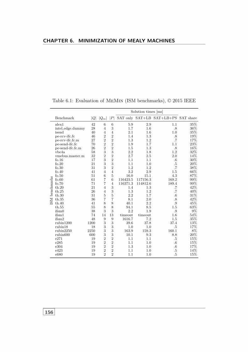
CHAPTER 6. MINIMIZATION OF MEALY MACHINES
Table 6.1: Evaluation of MeMin (ISM benchmarks), © 2015 IEEE
Solution times [ms]Benchmark |Q| |Qm| |P | SAT only SAT+LB SAT+LB+PS SAT share
ISM
benchm
arks
alex1 42 6 6 5.9 2.9 1.1 35%intel edge.dummy 28 4 3 1.7 1.6 .8 36%isend 40 4 4 2.1 1.6 1.0 35%pe-rcv-ifc.fc 46 2 2 1.4 1.3 .8 19%pe-rcv-ifc.fc.m 27 2 2 1.3 1.2 .7 17%pe-send-ifc.fc 70 2 2 1.9 1.7 1.1 23%pe-send-ifc.fc.m 26 2 2 1.5 1.3 .8 16%vbe4a 58 3 3 2.2 1.8 1.2 32%vmebus.master.m 32 2 2 2.7 2.5 2.0 14%fo.16 17 3 2 1.1 1.1 .6 30%fo.20 21 3 3 1.1 1.0 .5 20%fo.30 31 3 2 1.2 1.2 .7 38%fo.40 41 4 4 3.2 2.9 1.5 66%fo.50 51 6 5 16.0 15.1 4.3 87%fo.60 61 7 6 116423.5 117156.3 169.2 99%fo.70 71 7 4 116371.3 114812.6 189.4 99%th.20 21 4 3 1.4 1.3 .7 42%th.25 26 4 3 1.3 1.2 .7 40%th.30 31 5 5 2.2 1.7 .6 31%th.35 36 7 7 8.1 2.0 .8 42%th.40 41 8 8 40.1 2.2 .9 45%th.55 55 8 8 94.1 8.5 1.5 63%ifsm0 38 3 3 2.2 1.9 .9 9%ifsm1 74 14 13 timeout timeout 1.6 54%ifsm2 48 9 9 1616.7 7.2 1.5 35%rubin1200 1200 3 3 39.6 37.8 37.4 13%rubin18 18 3 3 1.0 1.0 .5 17%rubin2250 2250 3 3 163.9 159.3 160.1 8%rubin600 600 3 3 10.1 9.3 8.8 20%e271 19 2 2 1.1 1.1 .5 15%e285 19 2 2 1.1 1.0 .6 15%e304 19 2 2 1.3 1.0 .6 17%e423 19 2 2 1.1 1.0 .5 14%e680 19 2 2 1.1 1.0 .5 15%
156

6.6. EVALUATION
Table 6.2: Evaluation of MeMin (MCNC benchmarks), © 2015 IEEE
Solution times [ms]Benchmark |Q| |Qm| |P | SAT only SAT+LB SAT+LB+PS SAT share
MCNC
benchm
arks
bbara 10 7 7 7.8 1.4 .5 9%bbsse 16 13 13 timeout 8.1 .9 14%bbtas 6 6 6 2.2 1.2 .5 8%beecount 7 4 4 1.3 1.2 .5 11%cse 16 16 16 timeout 4.2 .8 13%dk14 7 7 7 10.1 1.6 .6 9%dk15 4 4 4 1.3 1.1 .5 8%dk16 27 27 27 timeout 32.7 .9 16%dk17 8 8 8 30.9 1.6 .5 9%dk27 7 7 7 5.8 1.3 .4 9%dk512 15 15 15 timeout 3.4 .5 12%donfile 24 1 1 1.0 1.0 .5 8%ex1 20 18 18 timeout 9.3 1.0 12%ex2 19 5 4 3.8 3.5 .9 48%ex3 10 4 2 1.6 1.6 .8 47%ex4 14 14 14 timeout 3.0 .5 13%ex5 9 3 2 1.1 1.0 .5 22%ex6 8 8 8 39.3 1.6 .5 11%ex7 10 3 3 1.1 1.0 .5 16%keyb 19 19 19 timeout 6.9 1.1 13%kirkman 16 16 16 timeout 5.9 2.1 9%lion9 9 4 4 1.2 1.0 .4 11%lion 4 4 4 1.2 1.0 .4 8%mark1 15 12 12 timeout 9.5 1.0 35%mc 4 4 4 1.2 1.0 .4 8%modulo12 12 1 1 1.0 .9 .4 8%opus 10 9 9 265.3 1.7 .5 10%planet1 48 48 48 timeout 78.7 1.4 26%planet 48 48 48 timeout 78.3 1.4 26%pma 24 24 24 timeout 8.1 .8 17%s1488 48 48 48 timeout 137.7 2.0 22%s1494 48 48 48 timeout 134.0 2.0 23%s1a 20 1 1 3.3 3.2 2.7 8%s1 20 20 20 timeout 8.3 1.0 15%s208 18 18 18 timeout 7.6 1.0 13%s27 6 5 5 1.7 1.2 .5 9%s298 218 135 135 timeout 5273.0 9.7 36%s386 13 13 13 timeout 3.0 .7 13%s420 18 18 18 timeout 8.7 1.0 13%s510 47 47 47 timeout 89.6 1.2 30%s820 25 24 24 timeout 16.6 1.5 15%s832 25 24 24 timeout 18.9 1.6 15%s8 5 1 1 .9 .9 .4 7%sand 32 32 32 timeout 32.9 1.5 18%scf 121 97 97 timeout 1492.3 3.3 45%shiftreg 8 8 8 37.6 1.7 .4 9%sse 16 13 13 timeout 8.2 .9 14%styr 30 30 30 timeout 29.4 1.2 17%tav 4 4 4 1.2 1.1 .5 7%tbk 32 16 16 timeout 35.5 3.5 6%tma 20 18 18 timeout 4.7 .7 20%train11 11 4 4 1.2 1.1 .5 12%train4 4 4 4 1.1 1.0 .4 8%
157

CHAPTER 6. MINIMIZATION OF MEALY MACHINES
benchmarks that we used in Section 6.6.1. ISM was slightly faster than BICAon only one benchmark (ifsm1 ). It was more than 100 times slower thanBICA on five benchmarks, and was unable to solve seven benchmarks thatBICA was able to solve.
Slim [HM96] is not available because it is Fujitsu’s proprietary [Hig15]. Also,the source code of VOID [AD01] is not available anymore [Ahm15]. Whilewe were able to obtain a copy of CHESMIN [GF07] from the authors, unfor-tunately, on our machine, the version we obtained yields segmentation faultson most benchmarks.
6.6.4 Experimental SetupAll experiments were run on an Intel Core i5-4590 (3.3GHz) with 4GB ofRAM. We disabled dynamic frequency scaling, and copied all executables andbenchmark files to a RAM disk, to minimize timing variations due to harddrive accesses. The execution times were measured using the perf tool [per].
We used BICA in version 5.0.3. We specified a hash table of size 100,000(parameter “-h 100,000”). With the default size of 10,000 some benchmarksfailed with the error message “Too many collisions. Specify a large hash table.”We used the version of STAMINA that is included in SIS 1.3.6 [Cho05]. Forthe exact mode, we specified the parameter “-s 0”, and for the heuristic mode“-s 3” (which combines the “tight upper bound” and “isomorphic” heuristics).We used a version of COSME (as of Aug. 2010) that was provided to us byone of the authors. We specified the same parameters as in the evaluationin [AS13] (“--comparemode --shownum --xincha”).
6.7 Conclusions and Future WorkWith respect to the set of benchmarks used to evaluate previous approaches,one can consider the problem of minimizing incompletely specified Mealymachines to be solved: Our method can solve all of these benchmarks in lessthan 0.2 seconds, and all but four in less than 10ms.
To evaluate the limits of our approach, one problem that future work willneed to address is to identify a new set of challenging, realistic benchmarks.
158

6.A. APPENDIX: COMPLETE BENCHMARK RESULTS
6.A Appendix: Complete Benchmark Results
159
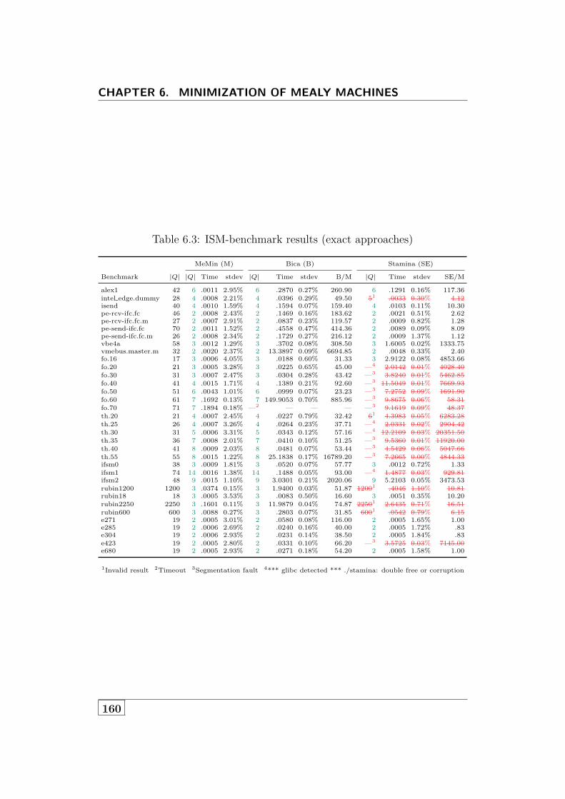
CHAPTER 6. MINIMIZATION OF MEALY MACHINES
Table 6.3: ISM-benchmark results (exact approaches)
MeMin (M) Bica (B) Stamina (SE)
Benchmark |Q| |Q| Time stdev |Q| Time stdev B/M |Q| Time stdev SE/M
alex1 42 6 .0011 2.95% 6 .2870 0.27% 260.90 6 .1291 0.16% 117.36intel edge.dummy 28 4 .0008 2.21% 4 .0396 0.29% 49.50 51 .0033 0.30% 4.12isend 40 4 .0010 1.59% 4 .1594 0.07% 159.40 4 .0103 0.11% 10.30pe-rcv-ifc.fc 46 2 .0008 2.43% 2 .1469 0.16% 183.62 2 .0021 0.51% 2.62pe-rcv-ifc.fc.m 27 2 .0007 2.91% 2 .0837 0.23% 119.57 2 .0009 0.82% 1.28pe-send-ifc.fc 70 2 .0011 1.52% 2 .4558 0.47% 414.36 2 .0089 0.09% 8.09pe-send-ifc.fc.m 26 2 .0008 2.34% 2 .1729 0.27% 216.12 2 .0009 1.37% 1.12vbe4a 58 3 .0012 1.29% 3 .3702 0.08% 308.50 3 1.6005 0.02% 1333.75vmebus.master.m 32 2 .0020 2.37% 2 13.3897 0.09% 6694.85 2 .0048 0.33% 2.40fo.16 17 3 .0006 4.05% 3 .0188 0.60% 31.33 3 2.9122 0.08% 4853.66fo.20 21 3 .0005 3.28% 3 .0225 0.65% 45.00 —4 2.0142 0.01% 4028.40fo.30 31 3 .0007 2.47% 3 .0304 0.28% 43.42 —3 3.8240 0.01% 5462.85fo.40 41 4 .0015 1.71% 4 .1389 0.21% 92.60 —3 11.5049 0.01% 7669.93fo.50 51 6 .0043 1.01% 6 .0999 0.07% 23.23 —3 7.2752 0.09% 1691.90fo.60 61 7 .1692 0.13% 7 149.9053 0.70% 885.96 —3 9.8675 0.06% 58.31fo.70 71 7 .1894 0.18% —2 — — — —3 9.1619 0.09% 48.37th.20 21 4 .0007 2.45% 4 .0227 0.79% 32.42 61 4.3983 0.05% 6283.28th.25 26 4 .0007 3.26% 4 .0264 0.23% 37.71 —4 2.0331 0.02% 2904.42th.30 31 5 .0006 3.31% 5 .0343 0.12% 57.16 —4 12.2109 0.03% 20351.50th.35 36 7 .0008 2.01% 7 .0410 0.10% 51.25 —3 9.5360 0.01% 11920.00th.40 41 8 .0009 2.03% 8 .0481 0.07% 53.44 —3 4.5429 0.06% 5047.66th.55 55 8 .0015 1.22% 8 25.1838 0.17% 16789.20 —3 7.2665 0.00% 4844.33ifsm0 38 3 .0009 1.81% 3 .0520 0.07% 57.77 3 .0012 0.72% 1.33ifsm1 74 14 .0016 1.38% 14 .1488 0.05% 93.00 —4 1.4877 0.03% 929.81ifsm2 48 9 .0015 1.10% 9 3.0301 0.21% 2020.06 9 5.2103 0.05% 3473.53rubin1200 1200 3 .0374 0.15% 3 1.9400 0.03% 51.87 12001 .4046 1.10% 10.81rubin18 18 3 .0005 3.53% 3 .0083 0.50% 16.60 3 .0051 0.35% 10.20rubin2250 2250 3 .1601 0.11% 3 11.9879 0.04% 74.87 22501 2.6435 0.71% 16.51rubin600 600 3 .0088 0.27% 3 .2803 0.07% 31.85 6001 .0542 0.79% 6.15e271 19 2 .0005 3.01% 2 .0580 0.08% 116.00 2 .0005 1.65% 1.00e285 19 2 .0006 2.69% 2 .0240 0.16% 40.00 2 .0005 1.72% .83e304 19 2 .0006 2.93% 2 .0231 0.14% 38.50 2 .0005 1.84% .83e423 19 2 .0005 2.80% 2 .0331 0.10% 66.20 —3 3.5725 0.03% 7145.00e680 19 2 .0005 2.93% 2 .0271 0.18% 54.20 2 .0005 1.58% 1.00
1Invalid result 2Timeout 3Segmentation fault 4*** glibc detected *** ./stamina: double free or corruption
160

6.A. APPENDIX: COMPLETE BENCHMARK RESULTS
Table 6.4: ISM-benchmark results (heuristic approaches)
Cosme (C) Stamina (SH)
Benchmark |Q| |Q| Time stdev C/M |Q| Time stdev SH/M
alex1 42 6 .0072 1.67% 6.54 6 .1361 0.09% 123.72intel edge.dummy 28 55 .0032 0.25% 4.00 55 .0048 0.25% 6.00isend 40 4 .0072 1.51% 7.20 4 .0125 0.19% 12.50pe-rcv-ifc.fc 46 2 .0083 0.33% 10.37 2 .0025 0.46% 3.12pe-rcv-ifc.fc.m 27 2 .0039 0.67% 5.57 2 .0010 0.57% 1.42pe-send-ifc.fc 70 2 .0224 0.42% 20.36 2 .0098 2.34% 8.90pe-send-ifc.fc.m 26 2 .0040 0.15% 5.00 2 .0009 0.80% 1.12vbe4a 58 3 .0163 0.36% 13.58 3 1.6815 0.02% 1401.25vmebus.master.m 32 2 .0113 0.65% 5.65 2 .0049 0.17% 2.45fo.16 17 3 .0015 0.88% 2.50 3 .0005 1.96% .83fo.20 21 3 .0018 0.26% 3.60 —6 .0009 1.64% 1.80fo.30 31 3 .0027 0.36% 3.85 —6 .0048 0.56% 6.85fo.40 41 65 .0040 0.32% 2.66 —6 .1386 0.05% 92.40fo.50 51 6 .0052 1.09% 1.20 —6 .0336 0.32% 7.81fo.60 61 105 .0093 2.15% .05 —6 .0864 1.23% .51fo.70 71 95 .0100 0.29% .05 —6 .1259 0.11% .66th.20 21 4 .0018 0.34% 2.57 —6 .0014 0.73% 2.00th.25 26 4 .0025 0.71% 3.57 —6 .0011 1.68% 1.57th.30 31 65 .0029 0.21% 4.83 —6 .0024 0.40% 4.00th.35 36 7 .0036 0.39% 4.50 —6 .0026 0.57% 3.25th.40 41 8 .0042 0.53% 4.66 —6 .0048 0.87% 5.33th.55 55 105 .0066 0.13% 4.40 —6 .0293 0.45% 19.53ifsm0 38 3 .0098 0.27% 10.88 3 .0012 0.81% 1.33ifsm1 74 14 .0140 0.12% 8.75 —6 .0026 0.31% 1.62ifsm2 48 31 .0058 0.41% 3.86 —6 .0024 0.37% 1.60rubin1200 1200 155 2.0928 0.05% 55.95 12005 .4101 1.43% 10.96rubin18 18 3 .0014 0.26% 2.80 3 .0004 2.01% .80rubin2250 2250 155 4.0188 0.06% 25.10 22505 2.6564 0.63% 16.59rubin600 600 155 1.1732 0.67% 133.31 6005 .0532 1.26% 6.04e271 19 2 .0020 0.41% 4.00 2 .0005 1.57% 1.00e285 19 2 .0019 0.27% 3.16 2 .0005 1.64% .83e304 19 195 .0021 0.35% 3.50 2 .0005 1.91% .83e423 19 195 .1175 0.04% 235.00 —6 .0017 0.58% 3.40e680 19 195 .0044 0.29% 8.80 2 .0005 1.69% 1.00
1Invalid result 5Result not minimal 6Other error
161

CHAPTER 6. MINIMIZATION OF MEALY MACHINES
Table 6.5: MCNC-benchmark results (exact approaches)
MeMin (M) Bica (B) Stamina (SE)
Benchmark |Q| |Q| Time stdev |Q| Time stdev B/M |Q| Time stdev SE/M
bbara 10 7 .0005 2.83% 7 .0252 0.14% 50.40 7 .0005 1.59% 1.00bbsse 16 13 .0009 1.73% 13 4.2474 0.03% 4719.33 13 .0006 1.30% .66bbtas 6 6 .0005 3.74% 6 .0015 0.87% 3.00 6 .0004 2.05% .80beecount 7 4 .0005 3.41% 4 .4787 0.11% 957.40 4 .0005 2.91% 1.00cse 16 16 .0008 2.03% 16 .0075 0.35% 9.37 16 .0005 1.71% .62dk14 7 7 .0006 2.82% 7 .0017 1.09% 2.83 7 .0004 2.06% .66dk15 4 4 .0005 3.22% 4 .0016 0.80% 3.20 4 .0004 2.65% .80dk16 27 27 .0009 2.09% 27 .0021 0.97% 2.33 27 .0005 1.24% .55dk17 8 8 .0005 3.34% 8 .0016 1.23% 3.20 8 .0004 4.12% .80dk27 7 7 .0004 3.44% 7 .0015 0.86% 3.75 7 .0004 1.83% 1.00dk512 15 15 .0005 2.81% 15 .0016 0.97% 3.20 15 .0004 1.65% .80donfile 24 1 .0005 3.92% 1 .0058 0.27% 11.60 1 .0006 2.64% 1.20ex1 20 18 .0010 1.82% 18 6.4799 0.03% 6479.90 18 .0008 1.63% .80ex2 19 5 .0009 2.00% 5 .1767 0.03% 196.33 141 .6162 0.15% 684.66ex3 10 4 .0008 2.24% 4 .0864 0.10% 108.00 51 .0028 0.50% 3.50ex4 14 14 .0005 2.57% 14 .0030 0.54% 6.00 14 .0004 1.90% .80ex5 9 3 .0005 3.09% 3 .0213 0.30% 42.60 41 .0008 0.92% 1.60ex6 8 8 .0005 3.28% 8 .0025 1.57% 5.00 8 .0004 2.13% .80ex7 10 3 .0005 3.45% 3 .0138 0.35% 27.60 41 .0013 0.42% 2.60keyb 19 19 .0011 1.64% 19 .0796 0.35% 72.36 19 .0008 2.97% .72kirkman 16 16 .0021 0.67% —7 .0007 1.24 .33 16 .0014 0.45% .66lion9 9 4 .0004 3.81% 4 .0156 0.61% 39.00 4 .0004 1.26% 1.00lion 4 4 .0004 3.91% 4 .0015 1.10% 3.75 4 .0004 1.77% 1.00mark1 15 12 .0010 1.72% 01 .0008 1.38% .80 12 .0006 1.44% .60mc 4 4 .0004 4.40% 4 .0015 0.52% 3.75 4 .0004 2.21% 1.00modulo12 12 1 .0004 4.27% 1 .0053 0.45% 13.25 —3 .0489 0.40% 122.25opus 10 9 .0005 3.07% 01 .0008 1.27% 1.60 9 .0004 1.60% .80planet1 48 48 .0014 1.49% 48 .3190 0.04% 227.85 48 .0006 1.40% .42planet 48 48 .0014 1.30% 48 .3190 0.01% 227.85 48 .0006 0.91% .42pma 24 24 .0008 2.20% 24 .0287 0.13% 35.87 —3 .0482 0.16% 60.25s1488 48 48 .0020 0.76% 48 .9242 0.08% 462.10 48 .0007 1.05% .35s1494 48 48 .0020 1.03% 48 .9369 2.64% 468.45 48 .0007 1.22% .35s1a 20 1 .0027 0.81% 1 .0558 0.06% 20.66 1 .0019 0.38% .70s1 20 20 .0010 1.50% 20 .1329 0.07% 132.90 20 .0005 2.48% .50s208 18 18 .0010 1.41% 18 .0462 0.05% 46.20 18 .0006 2.27% .60s27 6 5 .0005 3.32% 5 .0305 0.07% 61.00 5 .0004 2.12% .80s298 218 135 .0097 0.42% 135 34.2797 0.08% 3533.98 135 .0066 0.59% .68s386 13 13 .0007 2.24% 13 .0264 0.09% 37.71 13 .0004 1.85% .57s420 18 18 .0010 1.56% 18 .0642 0.04% 64.20 18 .0006 1.54% .60s510 47 47 .0012 1.47% —2 — — — 47 .0005 1.66% .41s820 25 24 .0015 2.02% —8 74.5850 0.70 49723.33 24 .0009 2.43% .60s832 25 24 .0016 1.37% —8 75.4407 1.01 47150.43 24 .0009 2.04% .56s8 5 1 .0004 3.90% 1 .0054 0.19% 13.50 1 .0004 1.64% 1.00sand 32 32 .0015 1.18% 32 19.4550 0.02% 12970.00 32 .0006 1.61% .40scf 121 97 .0033 0.72% —7 .0010 0.91 .30 97 .0027 0.34% .81shiftreg 8 8 .0004 3.90% 8 .0015 0.89% 3.75 8 .0004 2.15% 1.00sse 16 13 .0009 2.08% 13 4.2638 0.14% 4737.55 13 .0006 1.77% .66styr 30 30 .0012 1.39% 30 .2308 0.02% 192.33 30 .0006 1.78% .50tav 4 4 .0005 3.03% 4 .0020 1.21% 4.00 4 .0004 1.68% .80tbk 32 16 .0035 0.62% 16 .3170 0.06% 90.57 16 .0132 0.29% 3.77tma 20 18 .0007 2.51% 18 .0639 0.12% 91.28 —3 .0486 0.22% 69.42train11 11 4 .0005 3.91% 4 .0163 0.26% 32.60 4 .0004 2.60% .80train4 4 4 .0004 3.55% 4 .0016 1.38% 4.00 4 .0004 3.66% 1.00
1Invalid result 2Timeout 3Segmentation fault 7*Inconsistent machine detected. 8Out of memory
162

6.A. APPENDIX: COMPLETE BENCHMARK RESULTS
Table 6.6: MCNC-benchmark results (heuristic approaches)
Cosme (C) Stamina (SH)
Benchmark |Q| |Q| Time stdev C/M |Q| Time stdev SH/M
bbara 10 7 .0009 0.78% 1.80 7 .0005 1.81% 1.00bbsse 16 41 .0018 0.28% 2.00 13 .0007 1.06% .77bbtas 6 6 .0006 0.88% 1.20 6 .0004 2.04% .80beecount 7 31 .0008 0.94% 1.60 4 .0005 1.79% 1.00cse 16 51 .0020 0.38% 2.50 16 .0005 0.97% .62dk14 7 7 .0007 0.98% 1.16 7 .0004 2.22% .66dk15 4 4 .0006 1.11% 1.20 4 .0004 2.43% .80dk16 27 27 .0012 0.58% 1.33 27 .0005 1.56% .55dk17 8 8 .0006 0.60% 1.20 8 .0004 1.71% .80dk27 7 7 .0006 1.29% 1.50 7 .0004 1.32% 1.00dk512 15 15 .0027 0.39% 5.40 15 .0004 1.77% .80donfile 24 —8 287.4346 0.44 574869.20 1 .0006 3.21% 1.20ex1 20 61 .0033 0.41% 3.30 18 .0008 1.82% .80ex2 19 95 .0020 0.61% 2.22 —6 .0024 1.72% 2.66ex3 10 95 .0019 0.37% 2.37 —6 .0006 2.82% .75ex4 14 51 .0012 0.95% 2.40 14 .0004 1.66% .80ex5 9 85 .0009 1.13% 1.80 —6 .0005 1.65% 1.00ex6 8 21 .0010 0.58% 2.00 8 .0004 2.09% .80ex7 10 95 .0010 0.48% 2.00 —6 .0005 1.64% 1.00keyb 19 31 .0032 0.38% 2.90 19 .0008 1.12% .72kirkman 16 81 .0043 0.34% 2.04 16 .0014 0.25% .66lion9 9 4 .0010 0.72% 2.50 4 .0004 2.50% 1.00lion 4 21 .0006 0.72% 1.50 4 .0004 2.46% 1.00mark1 15 91 .0013 0.60% 1.30 12 .0006 1.36% .60mc 4 21 .0006 1.19% 1.50 4 .0004 3.48% 1.00modulo12 12 —8 207.9701 1.10 519925.25 —3 .0483 0.40% 120.75opus 10 41 .0011 0.59% 2.20 9 .0004 1.48% .80planet1 48 121 .0107 0.15% 7.64 48 .0006 1.97% .42planet 48 121 .0107 0.25% 7.64 48 .0006 1.33% .42pma 24 111 .0962 0.24% 120.25 —3 .0481 0.11% 60.12s1488 48 151 .0223 0.20% 11.15 48 .0007 1.17% .35s1494 48 141 .0227 0.12% 11.35 48 .0007 1.79% .35s1a 20 —2 — — — 1 .0020 0.43% .74s1 20 31 .0033 0.19% 3.30 20 .0005 1.34% .50s208 18 —2 — — — 18 .0006 3.40% .60s27 6 21 .0008 1.26% 1.60 5 .0004 1.40% .80s298 218 —2 — — — 135 .0066 0.34% .68s386 13 31 .0015 0.25% 2.14 13 .0004 1.51% .57s420 18 21 .0026 0.36% 2.60 18 .0006 1.58% .60s510 47 91 .0061 0.57% 5.08 47 .0005 1.34% .41s820 25 51 .0059 0.22% 3.93 24 .0009 1.36% .60s832 25 51 .0065 2.24% 4.06 24 .0009 0.69% .56s8 5 —8 144.1141 1.00 360285.25 1 .0004 3.78% 1.00sand 32 31 .0089 0.29% 5.93 32 .0006 1.67% .40scf 121 401 .0403 0.08% 12.21 97 .0028 0.40% .84shiftreg 8 8 .0007 1.80% 1.75 8 .0004 1.39% 1.00sse 16 41 .0018 0.28% 2.00 13 .0007 1.41% .77styr 30 111 .0057 0.23% 4.75 30 .0006 1.00% .50tav 4 —8 148.3782 0.23 296756.40 4 .0004 4.23% .80tbk 32 16 .0271 0.05% 7.74 16 .0133 0.16% 3.80tma 20 121 .0877 0.17% 125.28 —3 .0481 0.39% 68.71train11 11 4 .0012 0.57% 2.40 4 .0004 1.85% .80train4 4 4 .0005 0.41% 1.25 4 .0004 2.05% 1.00
1Invalid result 2Timeout 3Segmentation fault 5Result not minimal 6Other Error 8Out of memory
163


7Summary, Conclusions,
and Future Work
In this thesis, we have developed techniques to automatically generate modelsof microarchitectural components. Such models are, for example, importantfor building performance prediction tools, compilers, cycle-accurate simulators,and for showing the presence or absence of microarchitectural security issues.Previous approaches for obtaining microarchitectural models typically requireda significant amount of manual work, and the models were often not veryaccurate and precise.
7.1 Summary and Conclusions
7.1.1 Models of Recent MicroarchitecturesIn the first part of the thesis, we focused on recent x86 microarchitectures.
nanoBench
We have developed a general tool for evaluating small microbenchmarks usinghardware performance counters. Unlike previous tools, our tool can executemicrobenchmarks directly in kernel space. This makes it possible to benchmarkprivileged instructions, and it allows for more accurate measurements bydisabling interrupts and preemptions. The reading of the performance countersis implemented with minimal overhead, avoiding function calls and branches.Our tool is precise enough to measure individual memory accesses.
On top of nanoBench, we then developed techniques to automatically generatemicrobenchmarks for characterizing the performance of individual instructionsand for inferring properties of the cache architecture.
165

CHAPTER 7. SUMMARY, CONCLUSIONS, AND FUTURE WORK
Instruction Characterizations
We have presented an approach to automatically characterize the latency,throughput, and port usage of more than 13,000 instruction variants. Forthe latency, we have introduced a more precise definition that, in contrast toprevious definitions, considers dependencies between different pairs of inputand output operands. We have applied our approach to 16 different Intel andAMD microarchitectures. Our experimental evaluation demonstrates thatthe obtained instruction characterizations are both more accurate and moreprecise than those obtained by prior work.
Characterizing Cache Architectures
We have developed tools to analyze undocumented properties of caches. Inparticular, we have implemented two tools that can fully automatically infera large class of deterministic cache replacement policies. Furthermore, forcaches with nondeterministic policies, we have proposed tools that can help toidentify their policies manually. We have applied our techniques to 13 differentIntel microarchitectures, and we have found several previously undocumentedreplacement policies. Furthermore, we have discovered that flushing the cachedoes not necessarily reset the state of the replacement policy; this could beexploited to leak information in covert-channel or side-channel attacks.
7.1.2 General ModelsIn the second part of the thesis, we looked at more general techniques forobtaining models of hardware components. In particular, we have proposedthe problem of gray-box learning, in which learning algorithms can exploitknown information about the system to be learned. As a first step towardsolving this problem, we have developed an efficient learning algorithm forthe serial composition of two Mealy machines, in which the left machine isknown and the right machine is unknown.
While this was only a first step—applications to real-world systems willrequire support for more complex composition topologies—we were able toadapt a central idea of our learning algorithm to the problem of minimizingincompletely specified Mealy machines. We have implemented an exactminimization tool that outperforms previous exact approaches by severalorders of magnitude on a number of hard benchmarks and is even competitivewith state-of-the-art heuristic techniques.
166

7.2. FUTURE WORK
7.2 Future WorkThere are multiple directions for future work.
One direction is to develop microbenchmarks to build models of other per-formance-relevant components of microarchitectures, such as instructiondecoders, branch predictors, or translation lookaside buffers. Like the mi-crobenchmarks described in Chapters 3 and 4, these microbenchmarks couldbe evaluated using nanoBench.
Another direction is to adapt our techniques to non-x86 architectures, suchas ARM, MIPS, or RISC-V.
Furthermore, we would like to build tools that use the models we generatedin the first part of the thesis to predict or explain the performance of softwarerunning on the corresponding microarchitectures. We would also like tointegrate our models into existing tools, such as simulators like gem5 [BBB+11],or compilers like GCC [GCC] and LLVM [LA04].
In addition to that, we would like to implement and analyze microarchitecturalcovert-channel and side-channel attacks, in particular regarding the issuesdiscovered in Section 3.7.4 and Section 4.4.4.
Finally, we would like to close the gap between theory and practice byextending our gray-box learning approach to more complex compositiontopologies so that it can be applied to real-world systems.
167


Bibliography
[Abe12] Andreas Abel. Measurement-based inference of the cachehierarchy. Master’s thesis, Universität des Saarlandes, De-cember 2012. URL: http://embedded.cs.uni-saarland.de/literature/AndreasAbelMastersThesis.pdf. (Cited onpages 82, 83, 84, 86, 90, 111, and 112).
[ABu+19] A. C. Aldaya, B. B. Brumley, S. ul Hassan, C. Pereida García,and N. Tuveri. Port contention for fun and profit. In 2019IEEE Symposium on Security and Privacy (SP), pages 870–887,May 2019. doi:10.1109/SP.2019.00066. (Cited on page 76).
[AD01] Imtiaz Ahmad and A. Shoba Das. A heuristic algorithm forthe minimization of incompletely specified finite state machines.Computers & Electrical Engineering, 27(2):159–172, 2001. doi:10.1016/S0045-7906(00)00016-1. (Cited on pages 141, 145,151, 155, and 158).
[AFBKV15] Fides Aarts, Paul Fiterau-Brostean, Harco Kuppens, and FritsVaandrager. Learning register automata with fresh value gener-ation. In Proceedings of the 12th International Colloquium onTheoretical Aspects of Computing (ICTAC 2015), pages 165–183.Springer-Verlag, 2015. doi:10.1007/978-3-319-25150-9_11.(Cited on pages 17 and 118).
[Ahm01] Imtiaz Ahmad. A distributed algorithm for finding primecompatibles on network of workstations. Microprocessorsand Microsystems, 25(4):195–202, 2001. doi:10.1016/S0141-9331(01)00112-0. (Cited on pages 139 and 145).
[Ahm15] Imtiaz Ahmad. Personal communication, March 2015. (Citedon page 158).
[ALOJ13] Jung Ho Ahn, Sheng Li, Seongil O, and Norman P. Jouppi.McSimA+: A manycore simulator with application-level+ sim-ulation and detailed microarchitecture modeling. In 2013 IEEEInternational Symposium on Performance Analysis of Systemsand Software, Austin, TX, USA, pages 74–85, 2013. doi:10.1109/ISPASS.2013.6557148. (Cited on pages 40 and 79).
[AMD17] AMD. Software optimization guide for AMD family 17hprocessors. Publication No. 55723, Revision 3.00, June
169

BIBLIOGRAPHY
2017. URL: https://developer.amd.com/wordpress/media/2013/12/55723_SOG_Fam_17h_Processors_3.00.pdf. (Citedon pages 43 and 46).
[AMD19] AMD. AMD64 architecture programmer’s manual volume 2:System programming. Publication No. 24593, Revision 3.32,October 2019. URL: https://www.amd.com/system/files/TechDocs/24593.pdf. (Cited on page 74).
[Ang87] Dana Angluin. Learning regular sets from queries and counterex-amples. Information and computation, 75(2):87–106, Novem-ber 1987. doi:10.1016/0890-5401(87)90052-6. (Cited onpages 17, 118, 120, 134, and 145).
[AQH90] M. J. Avedillo, J. M. Quintana, and J. L. Huertas. New approachto the state reduction in incompletely specified sequential ma-chines. In IEEE International Symposium on Circuits and Sys-tems, pages 440–443, 1990. doi:10.1109/ISCAS.1990.112075.(Cited on page 146).
[AR12] Andreas Abel and Jan Reineke. Automatic cache modeling bymeasurements. In 6th Junior Researcher Workshop on Real-Time Computing (in conjunction with RTNS), November 2012.URL: http://embedded.cs.uni-saarland.de/publications/CacheModelingJRWRTC.pdf. (Cited on pages 86 and 111).
[AR13] Andreas Abel and Jan Reineke. Measurement-based modelingof the cache replacement policy. In 19th IEEE Real-Time andEmbedded Technology and Applications Symposium (RTAS),Philadelphia, PA, USA, April 9-11, 2013, pages 65–74, 2013.doi:10.1109/RTAS.2013.6531080. (Cited on pages 82, 83, 90,96, 111, and 112).
[AR14] Andreas Abel and Jan Reineke. Reverse engineering of cachereplacement policies in Intel microprocessors and their eval-uation. In 2014 IEEE International Symposium on Perfor-mance Analysis of Systems and Software (ISPASS), Monterey,CA, USA, March 23-25, 2014, pages 141–142, 2014. doi:10.1109/ISPASS.2014.6844475. (Cited on pages 19 and 79).
[AR15] Andreas Abel and Jan Reineke. MeMin: SAT-based exactminimization of incompletely specified Mealy machines. InProceedings of the IEEE/ACM International Conference onComputer-Aided Design (ICCAD), Austin, TX, USA, November
170

BIBLIOGRAPHY
2-6, 2015, ICCAD ’15, pages 94–101. IEEE Press, 2015. doi:10.1109/ICCAD.2015.7372555. (Cited on pages 19 and 139).
[AR16] Andreas Abel and Jan Reineke. Gray-box learning of serialcompositions of Mealy machines. In NASA Formal Methods—Proceedings of the 8th International Symposium, Minneapo-lis, MN, USA, June 7-9, 2016, NFM 2016, pages 272–287.Springer-Verlag, June 2016. doi:10.1007/978-3-319-40648-0_21. (Cited on pages 19 and 117).
[AR19] Andreas Abel and Jan Reineke. uops.info: Characterizinglatency, throughput, and port usage of instructions on Intelmicroarchitectures. In Proceedings of the Twenty-Fourth Inter-national Conference on Architectural Support for ProgrammingLanguages and Operating Systems (ASPLOS), Providence, RI,USA, April 13-17, 2019, ASPLOS ’19, pages 673–686. ACM,2019. doi:10.1145/3297858.3304062. (Cited on pages 19and 39).
[AR20] Andreas Abel and Jan Reineke. nanoBench: A low-overheadtool for running microbenchmarks on x86 systems. In IEEEInternational Symposium on Performance Analysis of Systemsand Software (ISPASS), Boston, MA, USA, August 23–25, 2020,August 2020. To appear. (Cited on pages 19, 21, and 79).
[AS09] A. Alberto and A. Simao. Minimization of incompletely specifiedfinite state machines based on distinction graphs. In 10th LatinAmerican Test Workshop (LATW ’09), pages 1–6, March 2009.doi:10.1109/LATW.2009.4813796. (Cited on page 140).
[AS13] Alex D. B. Alberto and Adenilso Simao. Iterative minimizationof partial finite state machines. Central European Journal ofComputer Science, 3(2):91–103, 2013. doi:10.2478/s13537-013-0106-0. (Cited on pages 141, 145, 146, 151, 154, and 158).
[Auf58] D. D. Aufenkamp. Analysis of sequential machines II. IRETransactions on Electronic Computers, EC-7(4):299–306, 1958.doi:10.1109/TEC.1958.5222663. (Cited on page 144).
[AZMM04] Hussein Al-Zoubi, Aleksandar Milenkovic, and MilenaMilenkovic. Performance evaluation of cache replacement poli-cies for the SPEC CPU2000 benchmark suite. In Proceedings ofthe 42nd annual Southeast regional conference, pages 267–272.ACM, 2004. doi:10.1145/986537.986601. (Cited on page 83).
171

BIBLIOGRAPHY
[BACD97] Jeff Bilmes, Krste Asanovic, Chee-Whye Chin, and Jim Demmel.Optimizing matrix multiply using PHiPAC: a portable, high-performance, ANSI C coding methodology. In Proceedings ofthe 11th International Conference on Supercomputing, ICS ’97,pages 340–347. Association for Computing Machinery, 1997.doi:10.1145/263580.263662. (Cited on page 79).
[BBB+11] Nathan L. Binkert, Bradford M. Beckmann, Gabriel Black,Steven K. Reinhardt, Ali G. Saidi, Arkaprava Basu, Joel Hest-ness, Derek Hower, Tushar Krishna, Somayeh Sardashti, Rathi-jit Sen, Korey Sewell, Muhammad Shoaib Bin Altaf, NilayVaish, Mark D. Hill, and David A. Wood. The gem5 sim-ulator. SIGARCH Computer Architecture News, 39(2):1–7,2011. doi:10.1145/2024716.2024718. (Cited on pages 40, 79,and 167).
[BBG+12] Ramon Bertran, Alper Buyuktosunoglu, Meeta S. Gupta, MarcGonzalez, and Pradip Bose. Systematic energy characteriza-tion of CMP/SMT processor systems via automated micro-benchmarks. In Proceedings of the 45th Annual IEEE/ACM In-ternational Symposium on Microarchitecture, MICRO-45, pages199–211, Washington, DC, USA, 2012. IEEE Computer Society.doi:10.1109/MICRO.2012.27. (Cited on page 40).
[BBS12] Domagoj Babic, Matko Botincan, and Dawn Song. Symbolicgrey-box learning of input-output relations. Technical ReportUCB/EECS-2012-59, University of California, Berkeley, May2012. URL: http://www.eecs.berkeley.edu/Pubs/TechRpts/2012/EECS-2012-59.html. (Cited on page 135).
[BC00] Josep M. Blanquer and Robert C. Chalmers. MOB: Amemory organization benchmark. Technical report, Uni-versity of California, Santa Barbara, October 2000. URL:http://www.gnu-darwin.org/www001/ports-1.5a-CURRENT/devel/mob/work/mob-0.1.0/doc/mob.ps. (Cited on pages 86and 111).
[Ben71] R. G. Bennetts. An improved method of prime C-class derivationin the state reduction of sequential networks. IEEE Transactionson Computers, 20(2):229–231, February 1971. doi:10.1109/T-C.1971.223221. (Cited on page 145).
[BF72] Alan W. Biermann and Jerome A. Feldman. On the synthesisof finite-state machines from samples of their behavior. IEEE
172

BIBLIOGRAPHY
Transactions on Computers, 21(6):592–597, June 1972. doi:10.1109/TC.1972.5009015. (Cited on page 145).
[BHLM13] Benedikt Bollig, Peter Habermehl, Martin Leucker, and Ben-jamin Monmege. A fresh approach to learning register au-tomata. In Proceedings of the 17th International Conference onDevelopments in Language Theory (DLT), pages 118–130, 2013.doi:10.1007/978-3-642-38771-5_12. (Cited on pages 17and 118).
[Bia18] Andrea Di Biagio. llvm-mca: a static performance analysistool, 2018. URL: http://lists.llvm.org/pipermail/llvm-dev/2018-March/121490.html. (Cited on pages 40 and 77).
[Bil] Olexa Bilaniuk. libpfc. URL: https://github.com/obilaniu/libpfc. (Cited on pages 22, 31, and 35).
[BKMO14] Gilles Barthe, Boris Köpf, Laurent Mauborgne, and MartínOchoa. Leakage resilience against concurrent cache attacks. InPrinciples of Security and Trust—Third International Confer-ence, POST 2014, Held as Part of the European Joint Con-ferences on Theory and Practice of Software, ETAPS 2014,Grenoble, France, pages 140–158, April 2014. doi:10.1007/978-3-642-54792-8_8. (Cited on page 114).
[BMME19] Samira Briongos, Pedro Malagón, José M. Moya, and ThomasEisenbarth. RELOAD+REFRESH: Abusing cache replacementpolicies to perform stealthy cache attacks, April 2019. arXiv:1904.06278. (Cited on pages 84, 112, and 115).
[BSN+19] Atri Bhattacharyya, Alexandra Sandulescu, MatthiasNeugschwandtner, Alessandro Sorniotti, Babak Falsafi, MathiasPayer, and Anil Kurmus. SMoTherSpectre: Exploitingspeculative execution through port contention. In Proceedingsof the 2019 ACM SIGSAC Conference on Computer andCommunications Security, CCS ’19, pages 785–800, New York,NY, USA, 2019. ACM. doi:10.1145/3319535.3363194. (Citedon page 76).
[BT09] Vlastimil Babka and Petr Tůma. Investigating cache parametersof x86 family processors. In Proceedings of the 2009 SPECbenchmark workshop, pages 77–96. Springer, 2009. doi:10.1007/978-3-540-93799-9_5. (Cited on pages 86 and 111).
173

BIBLIOGRAPHY
[BWL72] R. G. Bennetts, J. L. Washington, and D. W. Lewin. Acomputer algorithm for state table reduction. Radio andElectronic Engineer, 42(11):513–520, November 1972. doi:10.1049/ree.1972.0088. (Cited on page 145).
[C+10] Keith Cooper et al. The platform-aware compilation environ-ment, preliminary design document. Technical report, Depart-ment of Computer Science, Rice University, September 2010.URL: http://pace.rice.edu/uploadedFiles/Publications/PACEDesignDocument.pdf. (Cited on page 79).
[CBM+19] Yishen Chen, Ajay Brahmakshatriya, Charith Mendis, AlexRenda, Eric Atkinson, Ondrej Sykora, Saman Amarasinghe,and Michael Carbin. BHive: A benchmark suite and mea-surement framework for validating x86-64 basic block per-formance models. In 2019 IEEE International Symposiumon Workload Characterization (IISWC). IEEE, November2019. URL: http://groups.csail.mit.edu/commit/papers/19/ithemal-measurement.pdf. (Cited on page 36).
[CD01] C. L. Coleman and J. W. Davidson. Automatic memory hier-archy characterization. In IEEE International Symposium onPerformance Analysis of Systems and Software (ISPASS), pages103–110, November 2001. doi:10.1109/ISPASS.2001.990684.(Cited on pages 86 and 111).
[CGP03] Jamieson M. Cobleigh, Dimitra Giannakopoulou, and Corina S.Păsăreanu. Learning assumptions for compositional verification.In Tools and Algorithms for the Construction and Analysis ofSystems (TACAS), volume 2619 of Lecture Notes in ComputerScience, pages 331–346. Springer, 2003. doi:10.1007/3-540-36577-X_24. (Cited on page 118).
[Cho05] Philip Chong. SIS 1.3 unofficial distribution, November 2005.URL: https://ptolemy.berkeley.edu/projects/embedded/Alumni/pchong/sis.html. (Cited on page 158).
[CnKR17] Pablo Cañones, Boris Köpf, and Jan Reineke. Security anal-ysis of cache replacement policies. In Proceedings of the 6thInternational Conference on Principles of Security and Trust(POST), volume 10204, pages 189–209, Berlin, Heidelberg, 2017.Springer-Verlag. doi:10.1007/978-3-662-54455-6_9. (Citedon page 114).
174

BIBLIOGRAPHY
[CnKR19] Pablo Cañones, Boris Köpf, and Jan Reineke. On the incompa-rability of cache algorithms in terms of timing leakage. LogicalMethods in Computer Science, Volume 15, Issue 1, March 2019.doi:10.23638/LMCS-15(1:21)2019. (Cited on page 114).
[CRON+14] A. S. Charif-Rubial, E. Oseret, J. Noudohouenou, W. Jalby,and G. Lartigue. CQA: A code quality analyzer tool at bi-nary level. In 21st International Conference on High Per-formance Computing (HiPC), pages 1–10, December 2014.URL: http://www.maqao.org/publications/papers/CQA.pdf,doi:10.1109/HiPC.2014.7116904. (Cited on pages 40, 43,and 77).
[CS11] Keith Cooper and Jeffrey Sandoval. Portable techniques to findeffective memory hierarchy parameters. Technical report, RiceUniversity, 2011. URL: https://hdl.handle.net/1911/96399.(Cited on pages 86 and 111).
[CV14] Jie Chen and Guru Venkataramani. CC-Hunter: Uncov-ering covert timing channels on shared processor hardware.In Proceedings of the 47th Annual IEEE/ACM InternationalSymposium on Microarchitecture, MICRO-47, pages 216–228,Washington, DC, USA, 2014. IEEE Computer Society. doi:10.1109/MICRO.2014.42. (Cited on page 76).
[CWPD01] R. Clint Whaley, Antoine Petitet, and Jack J. Dongarra. Au-tomated empirical optimizations of software and the ATLASproject. In Parallel Computing, volume 27, pages 3–35. Else-vier, 2001. doi:10.1016/S0167-8191(00)00087-9. (Cited onpage 79).
[CX18] Keith Cooper and Xiaoran Xu. Efficient characterization ofhidden processor memory hierarchies. In Proceedings of the 18thInternational Conference on Computational Science (ICCS),Part III, pages 335–349, June 2018. doi:10.1007/978-3-319-93713-7_27. (Cited on pages 86 and 111).
[DK17] Goran Doychev and Boris Köpf. Rigorous analysis of softwarecountermeasures against cache attacks. In Proceedings of the38th ACM SIGPLAN Conference on Programming LanguageDesign and Implementation (PLDI), pages 406–421, New York,NY, USA, 2017. Association for Computing Machinery. doi:10.1145/3062341.3062388. (Cited on page 114).
175

BIBLIOGRAPHY
[DKMR15] Goran Doychev, Boris Köpf, Laurent Mauborgne, and JanReineke. CacheAudit: A tool for the static analysis of cacheside channels. ACM Transactions on Information and SystemSecurity (TISSEC), 18(1), June 2015. doi:10.1145/2756550.(Cited on page 114).
[DKPT17] Craig Disselkoen, David Kohlbrenner, Leo Porter, and DeanTullsen. PRIME+ABORT: A timer-free high-precision L3 cacheattack using Intel TSX. In Proceedings of the 26th USENIXConference on Security Symposium, SEC ’17, pages 51–67,Berkeley, CA, USA, 2017. USENIX Association. URL: http://dl.acm.org/citation.cfm?id=3241189.3241195. (Cited onpages 81 and 114).
[DLM+13] Anthony Danalis, Piotr Luszczek, Gabriel Marin, Jeffrey S. Vet-ter, and Jack Dongarra. BlackjackBench: Portable hardwarecharacterization with automated results’ analysis. The Com-puter Journal, 57(7):1002–1016, 06 2013. doi:10.1093/comjnl/bxt057. (Cited on pages 86 and 111).
[DMM+04] Jack J. Dongarra, Shirley Moore, Philip Mucci, Keith Seymour,and Haihang You. Accurate cache and TLB characterizationusing hardware counters. In Computational Science—ICCS2004, pages 432–439, 2004. doi:10.1007/978-3-540-24688-6_57. (Cited on pages 86 and 111).
[DSBC69] S. C. De Sarkar, A. K. Basu, and A. K. Choudhury. Simplifica-tion of incompletely specified flow tables with the help of primeclosed sets. IEEE Transactions on Computers, C-18(10):953–956, October 1969. doi:10.1109/T-C.1969.222552. (Cited onpage 145).
[DXS19] Shuwen Deng, Wenjie Xiong, and Jakub Szefer. A bench-mark suite for evaluating caches’ vulnerability to timing attacks.CoRR, abs/1911.08619, November 2019. arXiv:1911.08619.(Cited on page 114).
[EGPQ06] Edith Elkind, Blaise Genest, Doron Peled, and HongyangQu. Grey-box checking. In Formal Techniques for Net-worked and Distributed Systems (FORTE), pages 420–435, 2006.doi:10.1007/11888116_30. (Cited on page 135).
[EMRCS14] J. Echavarria, A. Morales-Reyes, R. Cumplido, and M. A. Salido.FSM merging and reduction for IP cores watermarking using
176

BIBLIOGRAPHY
genetic algorithms. In International Conference on ReConFig-urable Computing and FPGAs (ReConFig), pages 1–7. IEEE,December 2014. doi:10.1109/ReConFig.2014.7032525. (Citedon page 140).
[ENBSH11] David Eklov, Nikos Nikoleris, David Black-Schaffer, and ErikHagersten. Cache pirating: Measuring the curse of the sharedcache. In Proceedings of the 2011 International Conferenceon Parallel Processing, ICPP ’11, pages 165–175, Washing-ton, DC, USA, 2011. IEEE Computer Society. doi:10.1109/ICPP.2011.15. (Cited on pages 104 and 115).
[ES04] Niklas Eén and Niklas Sörensson. An extensible SAT-solver.In Theory and Applications of Satisfiability Testing, volume2919 of Lecture Notes in Computer Science, pages 502–518.Springer, 2004. doi:10.1007/978-3-540-24605-3_37. (Citedon page 149).
[Fal19] Brandon Falk. Sushi Roll: A CPU research kernel with minimalnoise for cycle-by-cycle micro-architectural introspection, Au-gust 2019. URL: https://gamozolabs.github.io/metrology/2019/08/19/sushi_roll.html. (Cited on page 37).
[FDTZ04] Basilio B. Fraguela, Ramon Doallo, Juan Tourino, and Emilio L.Zapata. A compiler tool to predict memory hierarchy perfor-mance of scientific codes. Parallel Computing, 30(2):225–248,2004. doi:10.1016/j.parco.2003.09.004. (Cited on page 114).
[Fin] FinalWire Ltd. AIDA64. URL: https://www.aida64.com/.(Cited on page 43).
[FJ05] M. Frigo and S. G. Johnson. The design and implementationof FFTW3. Proceedings of the IEEE, 93(2):216–231, 2005.doi:10.1109/JPROC.2004.840301. (Cited on page 79).
[Fog] Agner Fog. Test programs for measuring clock cycles and perfor-mance monitoring. URL: https://www.agner.org/optimize/.(Cited on pages 32 and 35).
[Fog19] Agner Fog. Instruction tables: Lists of instruction laten-cies, throughputs and micro-operation breakdowns for In-tel, AMD and VIA CPUs. Technical University of Den-mark, August 2019. URL: http://www.agner.org/optimize/instruction_tables.pdf. (Cited on pages 15, 40, 43, 48, 49,58, and 69).
177

BIBLIOGRAPHY
[FRMK19] Alireza Farshin, Amir Roozbeh, Gerald Q. Maguire, Jr., andDejan Kostić. Make the most out of last level cache in Intelprocessors. In Proceedings of the Fourteenth EuroSys Conference2019, EuroSys ’19, pages 8:1–8:17, New York, NY, USA, 2019.ACM. doi:10.1145/3302424.3303977. (Cited on page 81).
[GBK11] David Gullasch, Endre Bangerter, and Stephan Krenn. Cachegames – bringing access-based cache attacks on aes to practice.In Proceedings of the 2011 IEEE Symposium on Security andPrivacy, SP ’11, pages 490–505, USA, 2011. IEEE ComputerSociety. doi:10.1109/SP.2011.22. (Cited on page 114).
[GCC] GCC, the GNU compiler collection. URL: https://gcc.gnu.org/. (Cited on pages 40 and 167).
[GDTF+10] Jorge González-Domínguez, Guillermo L. Taboada, Basilio B.Fraguela, María J. Martín, and Juan Touriño. Servet: A bench-mark suite for autotuning on multicore clusters. In IPDPS, pages1–9. IEEE, 2010. doi:10.1109/IPDPS.2010.5470358. (Cited onpages 86 and 111).
[GF07] Sezer Gören and F. Joel Ferguson. On state reduction of in-completely specified finite state machines. Computers & Elec-trical Engineering, 33(1):58–69, January 2007. doi:10.1016/j.compeleceng.2006.06.001. (Cited on pages 141, 146, 151,and 158).
[Gin59] Seymour Ginsburg. On the reduction of superfluous statesin a sequential machine. J. ACM, 6(2):259–282, April 1959.doi:10.1145/320964.320983. (Cited on page 144).
[GJ11] Karthik Ganesan and Lizy K. John. MAximum MulticorePOwer (MAMPO): An automatic multithreaded syntheticpower virus generation framework for multicore systems. InProceedings of 2011 International Conference for High Perfor-mance Computing, Networking, Storage and Analysis, SC ’11,pages 53:1–53:12, New York, NY, USA, 2011. ACM. doi:10.1145/2063384.2063455. (Cited on page 40).
[GJB+10] Karthik Ganesan, Jungho Jo, W. Lloyd Bircher, DimitrisKaseridis, Zhibin Yu, and Lizy K. John. System-level max power(SYMPO): A systematic approach for escalating system-levelpower consumption using synthetic benchmarks. In Proceedingsof the 19th International Conference on Parallel Architectures
178

BIBLIOGRAPHY
and Compilation Techniques, PACT ’10, pages 19–28, New York,NY, USA, 2010. ACM. doi:10.1145/1854273.1854282. (Citedon page 40).
[GL65] A. Grasselli and F. Luccio. A method for minimizing the numberof internal states in incompletely specified sequential networks.IEEE Transactions on Electronic Computers, EC-14(3):350–359, June 1965. doi:10.1109/PGEC.1965.264140. (Cited onpages 140, 144, and 147).
[GL06] Olga Grinchtein and Martin Leucker. Learning finite-statemachines from inexperienced teachers. In Proceedings of the 8thInternational Conference on Grammatical Inference: Algorithmsand Applications, pages 344–345. Springer, 2006. doi:10.1007/11872436_30. (Cited on pages 134 and 145).
[GLP06] Olga Grinchtein, Martin Leucker, and Nir Piterman. Inferringnetwork invariants automatically. In Automated Reasoning,volume 4130 of Lecture Notes in Computer Science, pages 483–497. Springer, 2006. doi:10.1007/11814771_40. (Cited onpage 134).
[GMM16] Daniel Gruss, Clémentine Maurice, and Stefan Mangard.Rowhammer.js: A remote software-induced fault attack inJavaScript. In Proceedings of the 13th International Conferenceon Detection of Intrusions and Malware, and Vulnerability As-sessment, DIMVA 2016, pages 300–321. Springer-Verlag, 2016.doi:10.1007/978-3-319-40667-1_15. (Cited on page 114).
[GMWM16] Daniel Gruss, Clémentine Maurice, Klaus Wagner, and StefanMangard. Flush+Flush: A fast and stealthy cache attack. InProceedings of the 13th International Conference on Detection ofIntrusions and Malware, and Vulnerability Assessment, DIMVA2016, pages 279–299, Berlin, Heidelberg, 2016. Springer-Verlag.doi:10.1007/978-3-319-40667-1_14. (Cited on page 114).
[Goo] Google. EXEgesis. URL: https://github.com/google/EXEgesis. (Cited on page 43).
[GPY02] Alex Groce, Doron Peled, and Mihalis Yannakakis. Adaptivemodel checking. In Tools and Algorithms for the Constructionand Analysis of Systems (TACAS), volume 2280 of LectureNotes in Computer Science, pages 357–370. Springer, 2002.doi:10.1007/3-540-46002-0_25. (Cited on page 118).
179

BIBLIOGRAPHY
[GR08] Daniel Grund and Jan Reineke. Estimating the performanceof cache replacement policies. In Proceedings of the SixthACM/IEEE International Conference on Formal Methods andModels for Co-Design (MEMOCODE), pages 101–112. IEEE,2008. doi:10.1109/MEMCOD.2008.4547695. (Cited on page 113).
[Gra17] Torbjörn Granlund. Instruction latencies and throughput forAMD and Intel x86 processors, April 2017. URL: https://gmplib.org/~tege/x86-timing.pdf. (Cited on pages 40, 43,48, 71, and 72).
[GS06] Fei Guo and Yan Solihin. An analytical model for cache re-placement policy performance. In Proceedings of the JointInternational Conference on Measurement and Modeling ofComputer Systems, SIGMETRICS ’06/Performance ’06, pages228–239, New York, NY, USA, 2006. ACM. doi:10.1145/1140277.1140304. (Cited on page 113).
[GYCH18] Qian Ge, Yuval Yarom, David Cock, and Gernot Heiser. A sur-vey of microarchitectural timing attacks and countermeasureson contemporary hardware. Journal of Cryptographic Engineer-ing, 8(1):1–27, April 2018. doi:10.1007/s13389-016-0141-6.(Cited on pages 75, 76, and 114).
[GYLH16] Qian Ge, Yuval Yarom, Frank Li, and Gernot Heiser. Yourprocessor leaks information—and there’s nothing you can doabout it, 2016. arXiv:1612.04474. (Cited on page 110).
[H+10] Stefan Henkler et al. Legacy component integration by theFujaba real-time tool suite. In Proceedings of the 32ndACM/IEEE International Conference on Software Engineering,ICSE ’10, pages 267–270, New York, NY, USA, 2010. ACM.doi:10.1145/1810295.1810349. (Cited on page 135).
[HHEW15] Julian Hammer, Georg Hager, Jan Eitzinger, and GerhardWellein. Automatic loop kernel analysis and performancemodeling with Kerncraft. In Proceedings of the 6th Inter-national Workshop on Performance Modeling, Benchmark-ing, and Simulation of High Performance Computing Systems,PMBS ’15, pages 4:1–4:11, New York, NY, USA, 2015. ACM.doi:10.1145/2832087.2832092. (Cited on pages 40 and 77).
[Hig15] Hiroyuki Higuchi. Personal communication, March 2015. (Citedon page 158).
180

BIBLIOGRAPHY
[HKP15] Mohamed Hassan, Anirudh M. Kaushik, and Hiren D. Pa-tel. Reverse-engineering embedded memory controllers throughlatency-based analysis. In 21st IEEE Real-Time and EmbeddedTechnology and Applications Symposium, Seattle, WA, USA,pages 297–306, 2015. doi:10.1109/RTAS.2015.7108453. (Citedon page 111).
[HL11] Yating Hsu and David Lee. Machine learning for implantedmalicious code detection with incompletely specified systemimplementations. In IEEE International Conference on NetworkProtocols, pages 31–36, Washington, DC, USA, 2011. doi:10.1109/ICNP.2011.6089070. (Cited on page 134).
[HM95] Hiroyuki Higuchi and Yusuke Matsunaga. Implicit prime com-patible generation for minimizing incompletely specified finitestate machines. In Proceedings of the Asia and South PacificDesign Automation Conference, ASP-DAC ’95, New York, NY,USA, 1995. ACM. doi:10.1145/224818.224903. (Cited onpage 145).
[HM96] Hiroyuki Higuchi and Yusuke Matsunaga. A fast state reductionalgorithm for incompletely specified finite state machines. InProceedings of the 33rd Annual Design Automation Conference,DAC ’96, pages 463–466, New York, NY, USA, 1996. ACM.doi:10.1145/240518.240606. (Cited on pages 141, 145, 151,154, 155, and 158).
[Hop71] John Hopcroft. An n log n algorithm for minimizing states ina finite automaton. In Theory of Machines and Computations,pages 189–196. Academic Press, New York, 1971. doi:10.1016/B978-0-12-417750-5.50022-1. (Cited on pages 18 and 140).
[HSJC12] Falk Howar, Bernhard Steffen, Bengt Jonsson, and Sofia Cassel.Inferring canonical register automata. In Verification, ModelChecking, and Abstract Interpretation, volume 7148 of LectureNotes in Computer Science, pages 251–266. Springer, 2012. doi:10.1007/978-3-642-27940-9_17. (Cited on pages 17 and 118).
[HV10] Marijn J. H. Heule and Sicco Verwer. Exact DFA identifica-tion using SAT solvers. In Grammatical Inference: Theoret-ical Results and Applications, volume 6339 of Lecture Notesin Computer Science, pages 66–79. Springer, 2010. doi:10.1007/978-3-642-15488-1_7. (Cited on pages 128 and 131).
181

BIBLIOGRAPHY
[HWH13] Ralf Hund, Carsten Willems, and Thorsten Holz. Practicaltiming side channel attacks against kernel space ASLR. In2013 IEEE Symposium on Security and Privacy, pages 191–205. IEEE, 2013. doi:10.1109/SP.2013.23. (Cited on pages 81and 82).
[HXB04] Heng Hu, Hong-Xi Xue, and Ji-Nian Bian. HSM2: A new heuris-tic state minimization algorithm for finite state machine. Jour-nal of Computer Science and Technology, 19(5):729–733, Septem-ber 2004. doi:10.1007/BF02945600. (Cited on pages 141, 145,151, and 155).
[IES15] Gorka Irazoqui, Thomas Eisenbarth, and Berk Sunar. Sys-tematic reverse engineering of cache slice selection in Intelprocessors. In Proceedings of the 2015 Euromicro Confer-ence on Digital System Design, pages 629–636. IEEE, 2015.doi:10.1109/DSD.2015.56. (Cited on pages 81 and 82).
[IGI+16] Mehmet Sinan Inci, Berk Gulmezoglu, Gorka Irazoqui, ThomasEisenbarth, and Berk Sunar. Cache attacks enable bulk keyrecovery on the cloud. In International Conference on Cryp-tographic Hardware and Embedded Systems, pages 368–388.Springer, 2016. doi:10.1007/978-3-662-53140-2_18. (Citedon pages 81 and 82).
[IHS15] Malte Isberner, Falk Howar, and Bernhard Steffen. The open-source LearnLib. In Computer Aided Verification, pages 487–495.Springer, 2015. doi:10.1007/978-3-319-21690-4_32. (Citedon pages 17, 119, and 133).
[Ins] InstLatx64. x86, x64 instruction latency, memory latency andCPUID dumps. URL: http://instlatx64.atw.hu/. (Cited onpages 40, 43, and 69).
[Inta] Intel Corporation. Intel architecture code analyzer.URL: https://software.intel.com/en-us/articles/intel-architecture-code-analyzer. (Cited on pages 15, 41, 42,and 48).
[Intb] Intel Corporation. Intel VTune Amplifier. URL: https://software.intel.com/vtune. (Cited on pages 22 and 35).
[Intc] Intel Corporation. X86 Encoder Decoder (XED). URL: https://intelxed.github.io/. (Cited on pages 15, 41, and 61).
182

BIBLIOGRAPHY
[Int12] Intel Corporation. Intel 64 and IA-32 Architectures Optimiza-tion Reference Manual, April 2012. Order Number: 248966-026.URL: https://www.intel.com/content/dam/doc/manual/64-ia-32-architectures-optimization-manual.pdf. (Cited onpages 14, 40, 42, 47, 69, 70, and 71).
[Int19a] Intel Corporation. 10th generation Intel Core Processor—instruction throughput and latency README, September2019. URL: https://software.intel.com/en-us/download/10th-generation-intel-core-processor-instruction-throughput-and-latency-docs. (Cited on pages 42 and 64).
[Int19b] Intel Corporation. Intel 64 and IA-32 Architectures Opti-mization Reference Manual, September 2019. Order Number:248966-042b. URL: https://software.intel.com/sites/default/files/managed/9e/bc/64-ia-32-architectures-optimization-manual.pdf. (Cited on pages 14, 27, 40, 42, 44,47, 48, 53, 54, 62, 71, and 72).
[Int19c] Intel Corporation. Intel 64 and IA-32 Architectures Software De-veloper’s Manual, October 2019. Order Number: 325462-071US.URL: https://software.intel.com/sites/default/files/managed/39/c5/325462-sdm-vol-1-2abcd-3abcd.pdf.(Cited on pages 33, 43, 61, 70, and 74).
[JB07] Tobias John and Robert Baumgartl. Exact cache charac-terization by experimental parameter extraction. In Pro-ceedings of the 15th International Conference on Real-Timeand Network Systems (RTNS), pages 65–74, Nancy, France,2007. URL: https://hal.inria.fr/inria-00168530/file/actes.pdf#page=66. (Cited on pages 86 and 111).
[JEJI08] Ajay Joshi, Lieven Eeckhout, Lizy K. John, and Ciji Isen. Au-tomated microprocessor stressmark generation. In Interna-tional Symposium on High-Performance Computer Architecture-Proceedings, pages 209–219. IEEE Computer Society, February2008. doi:10.1109/HPCA.2008.4658642. (Cited on page 40).
[JGSW12] Sanjeev Jahagirdar, Varghese George, Inder Sodhi, and RyanWells. Power management of the third generation Intel Coremicro architecture formerly codenamed Ivy Bridge. 2012 IEEEHot Chips 24 Symposium (HCS), August 2012. doi:10.1109/hotchips.2012.7476478. (Cited on page 84).
183

BIBLIOGRAPHY
[JTSE10] Aamer Jaleel, Kevin B. Theobald, Simon C. Steely, Jr., and JoelEmer. High performance cache replacement using re-referenceinterval prediction (RRIP). In Proceedings of the 37th AnnualInternational Symposium on Computer Architecture, ISCA ’10,pages 60–71, New York, NY, USA, 2010. ACM. doi:10.1145/1815961.1815971. (Cited on pages 83, 84, 86, and 93).
[KAGPJ16] Mehmet Kayaalp, Nael Abu-Ghazaleh, Dmitry Ponomarev, andAamer Jaleel. A high-resolution side-channel attack on last-level cache. In Proceedings of the 53rd Annual Design Automa-tion Conference. ACM, 2016. doi:10.1145/2897937.2897962.(Cited on pages 81 and 82).
[KDK+14] Y. Kim, R. Daly, J. Kim, C. Fallin, J. H. Lee, D. Lee, C. Wilk-erson, K. Lai, and O. Mutlu. Flipping bits in memory with-out accessing them: An experimental study of DRAM distur-bance errors. In ACM/IEEE 41st International Symposiumon Computer Architecture (ISCA), pages 361–372, June 2014.doi:10.1109/ISCA.2014.6853210. (Cited on page 114).
[KHF+19] P. Kocher, J. Horn, A. Fogh, D. Genkin, D. Gruss, W. Haas,M. Hamburg, M. Lipp, S. Mangard, T. Prescher, M. Schwarz,and Y. Yarom. Spectre attacks: Exploiting speculative execu-tion. 2019 IEEE Symposium on Security and Privacy (SP),May 2019. doi:10.1109/sp.2019.00002. (Cited on pages 13and 22).
[KLA+18] Vladimir Kiriansky, Ilia Lebedev, Saman Amarasinghe, SrinivasDevadas, and Joel Emer. DAWG: A defense against cache timingattacks in speculative execution processors. In Proceedingsof the 51st Annual IEEE/ACM International Symposium onMicroarchitecture, MICRO-51, pages 974–987. IEEE Press, 2018.doi:10.1109/MICRO.2018.00083. (Cited on page 115).
[KMO12] Boris Köpf, Laurent Mauborgne, and Martín Ochoa. Auto-matic quantification of cache side-channels. In Proceedings ofthe 24th International Conference on Computer Aided Veri-fication, CAV ’12, pages 564–580, Berlin, Heidelberg, 2012.Springer-Verlag. doi:10.1007/978-3-642-31424-7_40. (Citedon page 114).
[KPD+11] Russell Kegley, Jonathan Preston, Brian Dougherty, JulesWhite, and Anirudda Gokhale. Predictive cache modelingand analysis. Technical report, Lockheed Martin Aeronautics
184

BIBLIOGRAPHY
Corporation, November 2011. URL: https://apps.dtic.mil/dtic/tr/fulltext/u2/a552968.pdf. (Cited on page 114).
[KPMR12] Taesoo Kim, Marcus Peinado, and Gloria Mainar-Ruiz.STEALTHMEM: System-level protection against cache-basedside channel attacks in the cloud. In Proceedings of the21st USENIX Security Symposium (USENIX Security 12),pages 189–204, USA, 2012. USENIX Association. URL:https://www.usenix.org/conference/usenixsecurity12/technical-sessions/presentation/kim. (Cited onpage 115).
[KS91] L. N. Kannan and D. Sarma. Fast heuristic algorithms for finitestate machine minimization. In Proceedings of the EuropeanConference on Design Automation., EURO-DAC ’91, pages192–196, Los Alamitos, CA, USA, February 1991. IEEE Com-puter Society Press. doi:10.1109/EDAC.1991.206388. (Citedon pages 141, 145, and 151).
[KS13] A. S. Klimowicz and V. V. Solov’ev. Minimization of incom-pletely specified Mealy finite-state machines by merging twointernal states. J. Comput. Syst. Sci. Int., 52(3):400–409, May2013. doi:10.1134/S106423071303009X. (Cited on pages 141,146, 151, and 155).
[KVBSV94] T. Kam, T. Villa, R. Brayton, and A. Sangiovanni-Vincentelli.A fully implicit algorithm for exact state minimization. In31st Conference on Design Automation, pages 684–690, June1994. doi:10.1109/DAC.1994.204189. (Cited on pages 141, 151,and 155).
[KVBSV10] Timothy Kam, Tiziano Villa, Robert K. Brayton, and Alberto L.Sangiovanni-Vincentelli. Synthesis of Finite State Machines:Functional Optimization. Springer Publishing Company, 1stedition, 2010. (Cited on page 145).
[LA04] Chris Lattner and Vikram Adve. LLVM: A compilation frame-work for lifelong program analysis & transformation. In Pro-ceedings of the International Symposium on Code Generationand Optimization: Feedback-directed and Runtime Optimization,CGO ’04, pages 75–86, Washington, DC, USA, 2004. IEEEComputer Society. doi:10.1109/CGO.2004.1281665. (Cited onpages 40, 42, and 167).
185

BIBLIOGRAPHY
[Lam73] Butler W. Lampson. A note on the confinement problem.Commun. ACM, 16(10):613–615, October 1973. doi:10.1145/362375.362389. (Cited on page 75).
[LD97] Stan Liao and Srinivas Devadas. Solving covering problems usingLPR-based lower bounds. In Proceedings of the 34th AnnualDesign Automation Conference (DAC), pages 117–120. ACM,June 1997. doi:10.1145/266021.266046. (Cited on page 145).
[Lee15] David Lee. Personal communication, January 2015. (Cited onpage 134).
[LGR+16] Mingsong Lv, Nan Guan, Jan Reineke, Reinhard Wilhelm,and Wang Yi. A survey on static cache analysis for real-timesystems. Leibniz Transactions on Embedded Systems, 3(1):05–1–05:48, 2016. doi:10.4230/LITES-v003-i001-a005. (Cited onpage 79).
[LHH+18] J. Laukemann, J. Hammer, J. Hofmann, G. Hager, andG. Wellein. Automated instruction stream throughput predic-tion for Intel and AMD microarchitectures. In 2018 IEEE/ACMPerformance Modeling, Benchmarking and Simulation of HighPerformance Computer Systems (PMBS), pages 121–131, LosAlamitos, CA, USA, November 2018. IEEE Computer Society.doi:10.1109/PMBS.2018.8641578. (Cited on page 40).
[LHHW19] Jan Laukemann, Julian Hammer, Georg Hager, and GerhardWellein. Automatic throughput and critical path analysis of x86and ARM assembly kernels. CoRR, abs/1910.00214, October2019. arXiv:1910.00214. (Cited on page 40).
[LHS+20] Moritz Lipp, Vedad Hadžić, Michael Schwarz, Arthur Perais,Clémentine Maurice, and Daniel Gruss. Take a way: Exploringthe security implications of AMD’s cache way predictors. InProceedings of the 15th ACM Asia Conference on Computer andCommunications Security (ASIA CCS). ACM, June 2020. Toappear. doi:10.1145/3320269.3384746. (Cited on page 114).
[LN12] Martin Leucker and Daniel Neider. Learning minimal determin-istic automata from inexperienced teachers. In ISoLA, pages524–538, 2012. doi:10.1007/978-3-642-34026-0_39. (Citedon page 134).
[LSG+18] Moritz Lipp, Michael Schwarz, Daniel Gruss, Thomas Prescher,Werner Haas, Stefan Mangard, Paul Kocher, Daniel Genkin,
186

BIBLIOGRAPHY
Yuval Yarom, and Mike Hamburg. Meltdown. CoRR, 2018.arXiv:1801.01207. (Cited on pages 13 and 22).
[LSX09] Gabriel H. Loh, Samantika Subramaniam, and Yuejian Xie.Zesto: A cycle-level simulator for highly detailed microarchitec-ture exploration. In Proceedings of the IEEE International Sym-posium on Performance Analysis of Systems and Software (IS-PASS), pages 53–64, 2009. doi:10.1109/ISPASS.2009.4919638.(Cited on pages 40 and 79).
[LT98] Enyou Li and Clark Thomborson. Data cache parameter mea-surements. In Proceedings of the International Conference onComputer Design: VLSI in Computers and Processors (ICCD),pages 376–383, Los Alamitos, CA, USA, October 1998. IEEE.doi:10.1109/ICCD.1998.727077. (Cited on pages 86 and 111).
[LYG+15] Fangfei Liu, Yuval Yarom, Qian Ge, Gernot Heiser, and Ruby B.Lee. Last-level cache side-channel attacks are practical. In IEEESymposium on Security and Privacy, pages 605–622. IEEE, 2015.doi:10.1109/SP.2015.43. (Cited on pages 81, 112, and 114).
[Man04] Stefan Manegold. The calibrator (v0.9e), a cache-memory andTLB calibration tool. http://homepages.cwi.nl/~manegold/Calibrator/, June 2004. (Cited on pages 86 and 111).
[MC17] Xinxin Mei and Xiaowen Chu. Dissecting GPU memory hier-archy through microbenchmarking. IEEE Trans. Parallel Dis-trib. Syst., 28(1):72–86, 2017. doi:10.1109/TPDS.2016.2549523.(Cited on page 111).
[McC18] John D. McCalpin. Comments on timing shortcode sections on Intel processors, July 2018. URL:https://sites.utexas.edu/jdm4372/2018/07/23/comments-on-timing-short-code-sections-on-intel-processors/.(Cited on page 33).
[Mea55] George H. Mealy. A method for synthesizing sequential circuits.The Bell System Technical Journal, 34(5):1045–1079, 1955. doi:10.1002/j.1538-7305.1955.tb03788.x. (Cited on page 144).
[Mee18] Hendrik Meerkamp. SUACA: A tool for performanceanalysis of machine programs. Bachelor thesis, SaarlandUniversity, July 2018. URL: http://compilers.cs.uni-saarland.de/publications/theses/meerkamp_bsc.pdf.(Cited on page 77).
187

BIBLIOGRAPHY
[MHSM09] Daniel Molka, Daniel Hackenberg, Robert Schöne, andMatthias S. Müller. Memory performance and cache coherencyeffects on an Intel Nehalem multiprocessor system. In Pro-ceedings of the 2009 18th International Conference on Par-allel Architectures and Compilation Techniques, PACT ’09,pages 261–270, Washington, DC, USA, 2009. IEEE. doi:10.1109/PACT.2009.22. (Cited on page 111).
[MM14] Oded Maler and Irini-Eleftheria Mens. Learning regular lan-guages over large alphabets. In Tools and Algorithms forthe Construction and Analysis of Systems (TACAS), volume8413 of Lecture Notes in Computer Science, pages 485–499.Springer, 2014. doi:10.1007/978-3-642-54862-8_41. (Citedon pages 17 and 118).
[MRAC19] Charith Mendis, Alex Renda, Saman Amarasinghe, and MichaelCarbin. Ithemal: Accurate, portable and fast basic blockthroughput estimation using deep neural networks. In Pro-ceedings of the 36th International Conference on MachineLearning, volume 97 of Proceedings of Machine Learning Re-search, pages 4505–4515, Long Beach, California, USA, June2019. PMLR. URL: http://proceedings.mlr.press/v97/mendis19a.html. (Cited on page 36).
[MS96] Larry McVoy and Carl Staelin. lmbench: portable tools forperformance analysis. In USENIX Annual Technical Confer-ence, pages 23–23, Berkeley, CA, USA, 1996. URL: http://dl.acm.org/citation.cfm?id=1268299.1268322. (Cited onpages 86 and 111).
[MSN+15] Clémentine Maurice, Nicolas Scouarnec, Christoph Neumann,Olivier Heen, and Aurélien Francillon. Reverse engineering Intellast-level cache complex addressing using performance counters.In Proceedings of the 18th International Symposium on Researchin Attacks, Intrusions, and Defenses, RAID 2015, pages 48–65,New York, NY, USA, 2015. Springer-Verlag New York, Inc.doi:10.1007/978-3-319-26362-5_3. (Cited on pages 81, 82,and 112).
[MWK17] Heiko Mantel, Alexandra Weber, and Boris Köpf. A systematicstudy of cache side channels across AES implementations. InProceedings of the 9th International Symposium on EngineeringSecure Software and Systems (ESSoS), pages 213–230. Springer,
188
BIBLIOGRAPHY
July 2017. doi:10.1007/978-3-319-62105-0_14. (Cited onpage 114).
[OST06] Dag Arne Osvik, Adi Shamir, and Eran Tromer. Cache attacksand countermeasures: The case of AES. In Proceedings of the2006 The Cryptographers’ Track at the RSA Conference on Top-ics in Cryptology, CT-RSA ’06, pages 1–20, Berlin, Heidelberg,2006. Springer-Verlag. doi:10.1007/11605805_1. (Cited onpage 114).
[Pao10] Gabriele Paoloni. How to benchmark code execution times on In-tel IA-32 and IA-64 instruction set architectures. Intel Corpora-tion, September 2010. URL: https://www.intel.com/content/dam/www/public/us/en/documents/white-papers/ia-32-ia-64-benchmark-code-execution-paper.pdf. (Cited onpage 32).
[per] perf: Linux profiling with performance counters. URL: https://perf.wiki.kernel.org. (Cited on pages 22, 35, and 158).
[Pfl73] C. P. Pfleeger. State reduction in incompletely speci-fied finite-state machines. IEEE Transactions on Comput-ers, C-22(12):1099–1102, December 1973. doi:10.1109/T-C.1973.223655. (Cited on pages 18, 140, and 144).
[PG93] R. Puri and Jun Gu. An efficient algorithm to search for mini-mal closed covers in sequential machines. IEEE Transactionson Computer-Aided Design of Integrated Circuits and Systems,12(6):737–745, June 1993. doi:10.1109/43.229748. (Cited onpages 141, 145, and 151).
[PJ15] Xiaoyue Pan and Bengt Jonsson. A modeling framework forreuse distance-based estimation of cache performance. In 2015IEEE International Symposium on Performance Analysis ofSystems and Software (ISPASS), pages 62–71. IEEE, March2015. doi:10.1109/ISPASS.2015.7095785. (Cited on page 83).
[PO99] J. M. Pena and A. L. Oliveira. A new algorithm for ex-act reduction of incompletely specified finite state machines.IEEE Transactions on Computer-Aided Design of IntegratedCircuits and Systems, 18(11):1619–1632, November 1999. doi:10.1109/43.806807. (Cited on pages 134, 141, 145, 149, 151,and 154).
189

BIBLIOGRAPHY
[PU59] M. C. Paull and S. H. Unger. Minimizing the number ofstates in incompletely specified sequential switching functions.IRE Transactions on Electronic Computers, EC-8(3):356–367,September 1959. doi:10.1109/TEC.1959.5222697. (Cited onpages 140 and 144).
[PWKJ16] Vincent Palomares, David C. Wong, David J. Kuck, and WilliamJalby. Evaluating out-of-order engine limitations using uopflow simulation. In Tools for High Performance Computing2015, pages 161–181. Springer International Publishing, 2016.doi:10.1007/978-3-319-39589-0_13. (Cited on page 40).
[QJP+07] Moinuddin K. Qureshi, Aamer Jaleel, Yale N. Patt, Simon C.Steely, and Joel Emer. Adaptive insertion policies for highperformance caching. In Proceedings of the 34th Annual In-ternational Symposium on Computer Architecture, ISCA ’07,pages 381–391, New York, NY, USA, 2007. Association forComputing Machinery. doi:10.1145/1250662.1250709. (Citedon page 86).
[RC13] Guillem Rueda Cebollero. Learning cache replacement poli-cies using register automata. Master’s thesis, Uppsala Uni-versity, Department of Information Technology, December2013. URL: http://www.diva-portal.org/smash/get/diva2:678847/FULLTEXT01.pdf. (Cited on pages 112 and 116).
[Rei08] Jan Reineke. Caches in WCET Analysis. PhD the-sis, Universität des Saarlandes, November 2008. URL:http://embedded.cs.uni-saarland.de/publications/DissertationCachesInWCETAnalysis.pdf. (Cited on pages 79and 111).
[RGBW07] Jan Reineke, Daniel Grund, Christoph Berg, and ReinhardWilhelm. Timing predictability of cache replacement poli-cies. Real-Time Systems, 37(2):99–122, November 2007. doi:10.1007/s11241-007-9032-3. (Cited on page 83).
[RHSJ94] June-Kyung Rho, G. D. Hachtel, F. Somenzi, and R. M. Ja-coby. Exact and heuristic algorithms for the minimizationof incompletely specified state machines. IEEE Transactionson Computer-Aided Design of Integrated Circuits and Systems,13(2):167–177, February 1994. doi:10.1109/43.259940. (Citedon pages 141, 145, and 151).
190

BIBLIOGRAPHY
[RS93] Ronald L. Rivest and Robert E. Schapire. Inference of finite au-tomata using homing sequences. Information and Computation,103(2):299–347, 1993. doi:10.1006/inco.1993.1021. (Cited onpages 132 and 134).
[RTHW14] T. Roehl, J. Treibig, G. Hager, and G. Wellein. Overhead analy-sis of performance counter measurements. In 43rd InternationalConference on Parallel Processing Workshops (ICCPW), pages176–185, September 2014. doi:10.1109/ICPPW.2014.34. (Citedon page 35).
[Rub75] Frank Rubin. Worst case bounds for maximal compatible sub-sets. IEEE Transactions on Computers, C-24(8):830–831, Au-gust 1975. doi:10.1109/T-C.1975.224315. (Cited on page 145).
[Set11] Burr Settles. From theories to queries: Active learning inpractice. In Active Learning and Experimental Design work-shop, in conjunction with AISTATS 2010, volume 16 of Pro-ceedings of Machine Learning Research, pages 1–18, Sardinia,Italy, 2011. PMLR. URL: http://proceedings.mlr.press/v16/settles11a.html. (Cited on page 118).
[SG09] Muzammil Shahbaz and Roland Groz. Inferring Mealy ma-chines. In Proceedings of the 2nd World Congress on FormalMethods, pages 207–222. Springer, 2009. doi:10.1007/978-3-642-05089-3_14. (Cited on pages 17 and 118).
[SGL95] J.M. Sanchez, A.O. Garnica, and J. Lanchares. A genetic algo-rithm for reducing the number of states in incompletely speci-fied finite state machines. Microelectronics journal, 26(5):463–470, 1995. doi:10.1016/0026-2692(95)98948-Q. (Cited onpages 141, 145, and 151).
[SK13] Daniel Sanchez and Christos Kozyrakis. ZSim: Fast and ac-curate microarchitectural simulation of thousand-core systems.In Proceedings of the 40th Annual International Symposium onComputer Architecture, ISCA ’13, pages 475–486, New York,NY, USA, 2013. ACM. doi:10.1145/2485922.2485963. (Citedon pages 40 and 79).
[SS95] Rafael H. Saavedra and Alan Jay Smith. Measuring cacheand TLB performance and their effect on benchmark runtimes.IEEE Transactions on Computers, 44(10):1223–1235, 1995. doi:10.1109/12.467697. (Cited on pages 86 and 111).
191

BIBLIOGRAPHY
[SSL+92] E. M. Sentovich, K. J. Singh, L. Lavagno, C. Moon, R. Mur-gai, A. Saldanha, H. Savoj, P. R. Stephan, Robert K.Brayton, and Alberto L. Sangiovanni-Vincentelli. SIS: Asystem for sequential circuit synthesis. Technical ReportUCB/ERL M92/41, EECS Department, University of California,Berkeley, 1992. URL: http://www2.eecs.berkeley.edu/Pubs/TechRpts/1992/2010.html. (Cited on pages 149 and 150).
[TASS09] David K. Tam, Reza Azimi, Livio B. Soares, and MichaelStumm. RapidMRC: approximating L2 miss rate curves oncommodity systems for online optimizations. In Proceedingsof the 14th international conference on Architectural supportfor programming languages and operating systems, ASPLOSXIV, pages 121–132, New York, NY, USA, 2009. ACM. doi:10.1145/1508244.1508259. (Cited on pages 113 and 114).
[THW10] Jan Treibig, Georg Hager, and Gerhard Wellein. LIKWID: Alightweight performance-oriented tool suite for x86 multicoreenvironments. In Proceedings of the International Conferenceon Parallel Processing Workshops, pages 207–216, Washington,DC, USA, 2010. IEEE. doi:10.1109/ICPPW.2010.38. (Cited onpage 35).
[TJYD10] Dan Terpstra, Heike Jagode, Haihang You, and Jack Dongarra.Collecting performance data with PAPI-C. In Tools for HighPerformance Computing 2009, pages 157–173. Springer, 2010.doi:10.1007/978-3-642-11261-4_11. (Cited on pages 22and 35).
[TLM18] Caroline Trippel, Daniel Lustig, and Margaret Martonosi. Melt-downPrime and SpectrePrime: Automatically-synthesized at-tacks exploiting invalidation-based coherence protocols. CoRR,abs/1802.03802, 2018. arXiv:1802.03802. (Cited on page 114).
[TY00] Clark Thomborson and Yuanhua Yu. Measuring datacache and TLB parameters under Linux. In Proceed-ings of the Symposium on Performance Evaluation ofComputer and Telecommunication Systems, pages 383–390,July 2000. URL: http://citeseerx.ist.psu.edu/viewdoc/summary?doi=10.1.1.36.1427. (Cited on pages 86 and 111).
[VGGK20] Pepe Vila, Pierre Ganty, Marco Guarnieri, and Boris Köpf.CacheQuery: Learning replacement policies from hardwarecaches. In Proceedings of the 41st ACM SIGPLAN Conference
192
BIBLIOGRAPHY
on Programming Language Design and Implementation (PLDI).Association for Computing Machinery, June 2020. To appear.(Cited on pages 90, 92, 105, 113, and 116).
[Vil15] Tiziano Villa. Personal communication, March 2015. (Cited onpage 155).
[Vil19] Pepe Vila. Personal communication, December 2019. (Cited onpage 109).
[VKBSV97] T. Villa, T. Kam, R. K. Brayton, and A. L. Sangiovanni-Vincentelli. Explicit and implicit algorithms for binate cov-ering problems. IEEE Transactions on Computer-Aided Designof Integrated Circuits and Systems, 16(7):677–691, July 1997.doi:10.1109/43.644030. (Cited on page 145).
[VKM19] Pepe Vila, Boris Köpf, and José F. Morales. Theory andpractice of finding eviction sets. In 2019 IEEE Symposiumon Security and Privacy (SP), pages 39–54, May 2019. doi:10.1109/SP.2019.00042. (Cited on pages 90 and 105).
[vSMK+20] Stephan van Schaik, Marina Minkin, Andrew Kwong, DanielGenkin, and Yuval Yarom. CacheOut: Leaking data on In-tel CPUs via cache evictions. https://cacheoutattack.com/,January 2020. (Cited on page 114).
[VSVA05] Abhay Vardhan, Koushik Sen, Mahesh Viswanathan, andGul Agha. Using language inference to verify omega-regularproperties. In Tools and Algorithms for the Constructionand Analysis of Systems (TACAS), volume 3440 of LectureNotes in Computer Science, pages 45–60. Springer, 2005. doi:10.1007/978-3-540-31980-1_4. (Cited on page 118).
[W+08] Reinhard Wilhelm et al. The worst-case execution timeproblem—overview of methods and survey of tools. ACM Trans-actions on Embedded Computing Systems (TECS), 7(3), 2008.doi:10.1145/1347375.1347389. (Cited on page 79).
[Wika] Skylake (client) - Microarchitectures - Intel. URL: https://en.wikichip.org/wiki/intel/microarchitectures/skylake_(client). (Cited on page 44).
[Wikb] Zen - Microarchitectures - AMD. URL: https://en.wikichip.org/wiki/amd/microarchitectures/zen.(Cited on page 46).
193

BIBLIOGRAPHY
[WL06] Zhenghong Wang and Ruby B. Lee. Covert and side chan-nels due to processor architecture. In Proceedings of the 22ndAnnual Computer Security Applications Conference (ACSAC),pages 473–482, Washington, DC, USA, December 2006. IEEEComputer Society. doi:10.1109/ACSAC.2006.20. (Cited onpage 76).
[WLPA14] Andrew Waterman, Yunsup Lee, David A. Patterson, and KrsteAsanović. The RISC-V instruction set manual, Volume I:User-level ISA, version 2.0. Technical Report UCB/EECS-2014-54, EECS Department, University of California, Berke-ley, May 2014. URL: http://www2.eecs.berkeley.edu/Pubs/TechRpts/2014/EECS-2014-54.html. (Cited on page 37).
[WM08] Vincent M. Weaver and Sally A. McKee. Can hardware per-formance counters be trusted? In 2008 IEEE InternationalSymposium on Workload Characterization, pages 141–150. IEEE,September 2008. doi:10.1109/IISWC.2008.4636099. (Cited onpage 33).
[Won13] Henry Wong. Intel Ivy Bridge cache replacement policy, Jan-uary 2013. URL: http://blog.stuffedcow.net/2013/01/ivb-cache-replacement/. (Cited on pages 86 and 112).
[WPSAM10] H. Wong, M.-M. Papadopoulou, M. Sadooghi-Alvandi, andA. Moshovos. Demystifying GPU microarchitecture through mi-crobenchmarking. In IEEE International Symposium on Perfor-mance Analysis of Systems and Software (ISPASS), pages 235–246, March 2010. doi:10.1109/ISPASS.2010.5452013. (Citedon page 111).
[WTM13] Vincent M. Weaver, Dan Terpstra, and Shirley Moore. Non-determinism and overcount on modern hardware performancecounter implementations. In IEEE International Sympo-sium on Performance Analysis of Systems and Software (IS-PASS), pages 215–224. IEEE, April 2013. doi:10.1109/ISPASS.2013.6557172. (Cited on page 33).
[XS20] Wenjie Xiong and Jakub Szefer. Leaking information throughcache LRU states. CoRR, abs/1905.08348v2, January 2020.arXiv:1905.08348v2. (Cited on page 115).
[Yan91] Saeyang Yang. Logic synthesis and optimization bench-marks user guide, Version 3.0. Technical report, Mi-
194

BIBLIOGRAPHY
croelectronics Center of North Carolina (MCNC), Jan-uary 1991. URL: http://citeseerx.ist.psu.edu/viewdoc/summary?doi=10.1.1.49.591&rank=1. (Cited on page 154).
[YF14] Yuval Yarom and Katrina Falkner. FLUSH+RELOAD: A highresolution, low noise, L3 cache side-channel attack. In 23rdUSENIX Security Symposium (USENIX Security 14), SEC ’14,pages 719–732, USA, 2014. USENIX Association. URL:https://www.usenix.org/conference/usenixsecurity14/technical-sessions/presentation/yarom. (Cited onpage 114).
[YGL+15] Yuval Yarom, Qian Ge, Fangfei Liu, Ruby B. Lee, and Ger-not Heiser. Mapping the Intel last-level cache. Cryptol-ogy ePrint Archive, Report 2015/905, 2015. URL: https://eprint.iacr.org/2015/905. (Cited on pages 81 and 82).
[YJS+06] Kamen Yotov, Sandra Jackson, Tyler Steele, Keshav Pingali,and Paul Stodghill. Automatic measurement of instruction cachecapacity. In Proceedings of the 18th International Workshop onLanguages and Compilers for Parallel Computing, pages 230–243. Springer, 2006. doi:10.1007/978-3-540-69330-7_16.(Cited on page 111).
[YPS05] Kamen Yotov, Keshav Pingali, and Paul Stodghill. Auto-matic measurement of memory hierarchy parameters. In SIG-METRICS, pages 181–192, New York, NY, USA, 2005. ACM.doi:10.1145/1064212.1064233. (Cited on pages 86 and 111).
[ZBW17] M. Zeiser, J. Betz, and D. Westhoff. Cache covert-channelmitigation in cloud virtualization with XEN’s credit scheduler.In IEEE Global Communications Conference, GLOBECOM2017, Singapore, pages 1–7, December 2017. doi:10.1109/GLOCOM.2017.8253984. (Cited on page 110).
[ZGY14] Yi Zhang, Nan Guan, and Wang Yi. Understanding the dynamiccaches on Intel processors: Methods and applications. In Pro-ceedings of the 12th IEEE International Conference on Embeddedand Ubiquitous Computing, EUC ’14, pages 58–64, USA, Au-gust 2014. IEEE Computer Society. doi:10.1109/EUC.2014.18.(Cited on page 112).
195


Index
µops, 45
active learning, 117, 118AES instructions, 69age graph, 92Angluin’s algorithm, 118, 145assembler, 25
black box, 118branch instructions, 58
cache, 79–116µop cache, 45associativity, 81block size, 81C-Box, 81cache set, 81congruent addresses, 82hash function, 81, 82hit, 81index, 81miss, 81organization, 81–82prefetching, 33slice, 81way, 81
cacheInfo, 86cacheSeq, 88chain instruction, 52CLFLUSH instruction, 89, 110closure, 148CNF, 128compatibility
rows, 124, 129states, 143, 148words, 122
covert channel, 75, 110, 114CPUID instruction, 32
decoder, 45dependency chain, 52
division, 46, 58
encoding, 25equivalence query, 118error state, 126, 131eviction set, 90execution port, see portexplicit operand, 25
functional unit, 46
gray-box learning, 117–138
hardware performance counters, seeperformance counters
hyper-threading, 33, 75
IACA, 42, 63implicit operand, 25, 62incompatibility matrix, 147initialization sequence, 89instruction variant, 62interference, 33ISM benchmarks, 151
L∗ algorithm, 118, 145latency
algorithm, 52–59definition, 47
LFENCE instruction, 32LLVM, 42loop unrolling, 29
MCNC benchmarks, 151, 154Mealy machine
completely specified, 119, 142definition, 119, 142incompletely specified, 142minimization, 139–164serial composition, 118, 120
measurements, 62MeMin, 139–164
197

INDEX
memory operand, 25micro-operation, 45microbenchmark, 22move elimination, 45
nanoBench, 21–37features, 25–32implementation, 32–34kernel mode, 29noMem mode, 30user mode, 29
observation table, 123closed, 125consistent, 124input-complete, 126p-closed, 125unique, 126
out-of-order execution, 46output query, 118
partial solution, 130, 149partition, 124, 128
closed, 125performance counters, 23–24
APERF/MPERF, 24core, 24fixed-function, 24programmable, 24uncore, 24, 82
permutation policy, 82, 90physically-contiguous memory, 34pipe, 46pipeline, 44–46
AMD, 46Intel, 44–46
port, 46combination, 48usagealgorithm, 49–51definition, 48
RDMSR instruction, 24RDPMC instruction, 24renamer, 45reorder buffer, 45replacement policy, 82
LRU3PLRU4, 96PLRU8Rand2, 102Rand3PLRU8, 102adaptive, 86, 92FIFO, 82LRU, 82MRU, 83NRU, 83permutation policy, 82, 90PLRU, 82QLRU, 83, 96, 104RRIP, 83
reservation station, 46reset sequence, 92, 110reset state, 142, 150right-equivalence, 120, 131
SAT, 128, 147scheduler, 46serializing instructions, 32SHL instruction, 73side channel, 75, 110, 114SIMD, 54status flags, 25, 56–58, 73
throughputalgorithm, 59–61definition, 47
uops.info, 39–77
WBINVD instruction, 89, 109
x86assembler, 25instruction set, 61
XML file, 63
zero idiom, 45, 54, 72
198