Automatic Fuel Injection Mapping for Small Two-Stroke Engines. · Whereas four-stroke engines have...

www.power4flight.com

Automatic Fuel Injection Mapping for Small Two-Stroke Engines.

Bill Vaglienti

Power4Flight


202 Wasco Loop, Suite 104

Hood River, OR 97031

541-308-0650

April 4, 2016

http://www.power4flight.com/


Abstract

This paper describes a process for developing the fuel injection settings for small air-cooled two-stroke engines. A personal computer commands a motoring dynamometer and engine control unit (ECU) to determine the optimum fuel and ignition for every combination of throttle position and engine speed. The fuel and ignition settings are determined based upon real time measurement of the brake power and specific fuel consumption. The engine map is optimized for power at certain operating points and for specific fuel consumption at other operating points. Computationally determining the ECU settings increases the repeatability of the engine mapping process, and reduces the time required for calibration. In addition, a detailed log of the engine performance as a function of the fuel and ignition settings is created for every operating point.



I. TABLE OF CONTENTS

I. Table of Contents ...................................................................................................................... 3

II. Fuel injecting small two-stroke engines ................................................................................... 1

III. Equipment ................................................................................................................................. 1

A. Motoring Dynamometer ...................................................................................................... 1

B. Engine Control Unit .............................................................................................................. 1

C. Metering fuel pump ............................................................................................................. 2

D. Cooling Fan ........................................................................................................................... 2

E. Two-stroke engine ............................................................................................................... 2

F. Control Computer ................................................................................................................ 2

IV. The engine map ........................................................................................................................ 2

A. Fuel ....................................................................................................................................... 2

B. Ignition advance ................................................................................................................... 3

V. Typical engine mapping ............................................................................................................ 3

VI. Automatic engine mapping overview ....................................................................................... 4

VII. Details of fuel mapping ............................................................................................................. 4

A. Key measurement data ........................................................................................................ 4

B. Data acquisition details ........................................................................................................ 5

C. The data plot ........................................................................................................................ 5

D. Maximum power versus best fuel economy ....................................................................... 7

E. Finding fuel for best SFC ...................................................................................................... 8

F. Fuel for best power .............................................................................................................. 9

G. Fuel search strategy ............................................................................................................. 9

VIII. Details of ignition advance mapping ................................................................................. 12

A. Ignition advance search strategy ....................................................................................... 12

B. Ignition selection for best power ....................................................................................... 12

C. Ignition selection for drivability ......................................................................................... 13

IX. Data smoothing and outliers .................................................................................................. 14

A. Curve fitting ....................................................................................................................... 14

B. Outliers ............................................................................................................................... 14

C. Increasing point density ..................................................................................................... 14



X. Logged data reprocessing ....................................................................................................... 15

A. Log data fields .................................................................................................................... 16

XI. Performance report generation .............................................................................................. 17

A. Raw Power ......................................................................................................................... 17

B. Corrected Power ................................................................................................................ 18

C. Fuel flow ............................................................................................................................. 19

XII. Challenges to automatic engine mapping .............................................................................. 20

A. Engine cooling .................................................................................................................... 20

B. Accounting for humidity .................................................................................................... 20

C. Handling faults ................................................................................................................... 21



Page 1

II. FUEL INJECTING SMALL TWO-STROKE ENGINES

The benefits of fuel injection over carburetion are numerous, particularly for aerospace applications where the atmospheric conditions can vary drastically. However, fuel injection on small two-stroke engines remains rare, and has significant challenges compared to the typical automotive fuel injection application.

Whereas four-stroke engines have valves that largely segregate intake air from exhaust gas, two-stroke engine exhaust is contaminated by induction air and fuel charge. This exhaust contamination in addition to a nominally richer required setting prohibits the use of an oxygen sensor or wideband oxygen sensor to adjust the fueling in real time. In addition, the low cylinder count causes the manifold pressure to vary significantly over the engine cycle, and to only weakly correlate to the quantity of air the engine is pumping. The poor manifold pressure signal prohibits its use as a primary input to the fueling tables of the engine control unit (ECU).

As a result, single and twin cylinder engines typically use the N-alpha method of fuel injection: the quantity of fuel injected is primarily based upon the speed of the engine (N) and the position of the throttle (alpha). Temperature and pressure measurements compensate for changes in the atmospheric conditions. In order to get good performance across the full range of operating conditions careful calibration must be performed on a dynamometer to precisely characterize the performance of the engine (including its induction and exhaust system) as a function of throttle and speed.

This paper describes a process for automatically calibrating the fuel injection system of small two-stroke engines.

III. EQUIPMENT

A. Motoring Dynamometer

The motoring dynamometer (dyno) is the TigerDyne from Currawong Engineering. This dyno is designed specifically for small engines. It can spin the engine in either direction at any speed up to 10000 RPM, independent of the shaft power produced by the engine. The dyno is supported on air bearings, and the torque reaction is measured with a load cell. Power measurements are typically repeatable within a few Watts. The dyno is controlled over Ethernet by software on a personal computer.

B. Engine Control Unit

The ECU is the CE367B from Currawong Engineering. This ECU is designed for small engine aerospace applications and provides all of the necessary interfaces to manage the engine, including the fuel and ignition systems. Sensors include throttle position, manifold pressure, manifold temperature, barometric pressure, cylinder head temperature, crank sensor, and fuel pressure. A controller area network (CAN) is used to connect the ECU to the host vehicle and the control computer.


http://www.currawongeng.com/products/dynamometer/

http://www.currawongeng.com/products/uav_engines/ecu/


Page 2

C. Metering fuel pump

A three-cylinder positive displacement fuel pump is used to provide fuel at constant pressure (typically at 3 bar) to the injector. The pump is the CD822 from Currawong Engineering. An encoder on the pump motor shaft measures the speed and number of rotations of the pump, which is converted into a fuel flow measurement. CAN bus is used to connect the pump to the ECU and control computer.

D. Cooling Fan

A centrifugal fan controlled by a variable frequency drive provides cooling air. The fan ducting blows air over the cylinder head of the engine. The fan drive is controlled over Ethernet by software on a personal computer. When connected to an ECU the control computer can drive the fan to target a specific cylinder head temperature.

E. Two-stroke engine

The automatic engine mapping process has been applied to a variety of small single cylinder two-stroke engines ranging in size from 29cc to 60cc. Each engine is integrated with an ECU and associated peripherals. The process should be applicable to any engine that fits the TigerDyne and CE367B.

F. Control Computer

The control computer is a Windows PC running custom software. The software establishes a connection to the dyno, the cooling fan, the fuel pump, and the ECU.

IV. THE ENGINE MAP

The ECU calibration settings are collectively referred to as the “map”. The pieces of map that we are concerned with are the fuel table and the ignition advance table.

A. Fuel

The fuel table is two-dimensional, with rows indicating throttles and columns indicating RPMs (Figure 1). The ECU determines the amount of fuel to inject on each cycle based upon its estimate of the mass air consumption of the engine. In the CE367B ECU the fuel table provides an estimate of the volume of air that is consumed, as a percentage of the piston swept volume per revolution1. The ECU combines this estimate with its other sensors to estimate the mass of air consumed, and hence the amount of fuel that should be injected.

1 Internally we refer to this as the volumetric efficiency (VE), however it is just a number that determines fuel flow. When all other variables are held constant the fuel flow is proportional to the fuel table number.


http://www.currawongeng.com/products/uav_engines/fuel-pumps/triplex/


Page 3

B. Ignition advance

The ignition advance table uses the same two-dimensional layout as the fuel table, with rows indicating throttles and columns indicating RPMs. There is no requirement for the ignition advance table to use the same rows and columns as the fuel table. The ignition advance table gives the crankshaft angle in degrees before top dead center where the ignition spark is triggered.

Figure 1 - The fuel table for a 50cc single-cylinder two-stroke

V. TYPICAL ENGINE MAPPING

Typically, the ECU map is developed on a dyno with an operator manually optimizing the fuel and ignition for each throttle and engine speed. The operator must simultaneously:

Get the engine and dynamometer on condition (throttle and speed)

Manage the engine temperature by adjusting cooling air flow

Observe and log the measured performance (power, fuel flow, exhaust gas data, etc.)

Vary the fuel and ignition values to determine optimum settings

Monitor the total system to prevent catastrophic failures of the engine or dyno

The operator starts by tuning the ECU for maximum power. They may then reduce the fuel (“lean”) to deliver lower specific fuel consumption (SFC)2. It is difficult to know how far to lean the engine before problems with engine performance and drivability will appear. To help with

2 If the fueling is optimized for maximum power, then by definition adding more fuel can only make the SFC worse. However, reducing fuel may improve the SFC if the loss of power is less than the reduction in fuel.

RPMs Throttles



Page 4

this the operator monitors the exhaust gases. Various rules of thumb are used to understand the combustion based on the exhaust gas data. However, the use of exhaust gas data is fraught with problems: the gases are contaminated by induction air, the analyzers require careful calibration, and as much as 60 seconds are required to get a reliable measurement after a fueling change is made.

The entire mapping process demands many hours of a highly skilled operator. If a change is made to the engine design, a new map must be developed. The large amount of labor required often dictates resolution in the map which is less than ideal, simply to reduce the amount of labor.

VI. AUTOMATIC ENGINE MAPPING OVERVIEW

In automatic engine mapping we attempt to remove the human operator, and let the control computer directly control the dyno, throttle, cooling fan, and ECU settings. Power measurements are used to determine the engine performance and select the correct fuel and ignition values.

The calibration process starts by downloading the existing fuel table from the ECU. The engine mapping software on the control computer commands the dyno speed and the engine throttle to match a location in the fuel table. The control computer then commands changes to the fuel table and measures the resulting performance change. A sophisticated algorithm decides on the optimum fuel based on this collected data. The control computer then changes the throttle and dyno speed to move to the next point, and repeats the process until all the desired cells of the fuel table have been determined. Each data point is logged to a file for post-run analysis. Once a basic fuel table is completed the ignition advance is determined. Since the correct amount of fuel does not substantially change with ignition advance3, the advance is simply chosen to provide maximum power without exceeding a set advance limit. As with the fuel table, each data point is logged to a file for post-run analysis.

VII. DETAILS OF FUEL MAPPING

A. Key measurement data

For each fuel flow that is tested three key measurements are made from the data. The first is the average power during the sampling window. The second measurement is the power standard deviation during the sampling window. The third measurement is the specific fuel consumption (SFC), and requires further discussion.

Specific fuel consumption is fuel consumption of the engine in grams per hour divided by the power of the engine in kilowatts. Lower SFCs represent better efficiency. Typical numbers for small two-strokes are 400 to 800 g/kW-hr. Note that the SFC is always computed with the raw

3 We’ve tested the assertion that fuel and ignition are decoupled. Although the ignition advance can dramatically change the amount of power the engine makes, the change to the fuel required is modest. If some coupling is expected then the mapping process would optimize fuel, then ignition, and then re-optimize fuel.



Page 5

power, since the fuel injected is already adjusted for the atmospheric conditions measured by the ECU.

Computing SFC requires an accurate measurement of fuel flow, which will typically take 20 to 30 seconds of averaging4. To reduce the amount of time needed to make the SFC measurement we replace fuel flow with the number from the fuel table. At fixed operating conditions the amount of fuel injected per second is directly proportional to this number, which the control computer already knows. The resulting measurement is called pseudo SFC (pSFC). All data analysis for purposes of calibration are done using the pSFC to speed up the data acquisition.

B. Data acquisition details

For each data point the control software changes the fuel in the table, waits a settling period, then begins sampling data - recording all measurements until the sample window ends. The average power and the standard deviation of the power are computed. The settling time must account for the engine response time to the fueling change, and the time constant of the power measurement. Typical settling times are between two and five seconds; however, when going from large to small fuel flows (rich to lean) the settling time is increased to give the excess fuel that may have accumulated in the manifold and crankcase time to be consumed.

The dyno power measurement sample rate is 20 Hz. The measurement has an analog 2nd order low-pass filter at 3 Hz. The averaging window is typically two to five seconds, providing between 40 and 100 power samples. The actual settling and sampling times are parameters that the operator can configure to choose between speed and fidelity. In aggregate, a 20 point fuel sweep will typically take 100 to 200 seconds.

The engine temperatures, the pressures, cooling fan speed, and the actual fuel flow are recorded in addition to the power. The measured fuel flow is not expected to be reliable over such short sampling windows; but is recorded for the sake of completeness.

C. The data plot

As the data are acquired during the fuel sweep a real time plot is created which shows power on the left axis and pSFC on the right (Figure 2). In addition to the raw data a smoothed and resampled version of the power and pSFC curves are plotted. The user can configure the smoothing function parameters, including the amount of smoothing and the percentage of points that are discarded as outliers. The plot also includes the power standard deviation information.

4 Fuel flows for these small engines are of the order of 0.1 grams per second. In order to find the optimum SFC we need to measure this to about 1% accuracy. Hence the long time needed to make a good measurement.



Page 6

Figure 2 - fuel data plot for a DA50 at 50% throttle and RPM of 5000

The smoother is critical to showing the trends of the performance as a function of fuel, thereby reducing the density of points that must be sampled. Since we assume the response to fuel changes should be smooth, the data smoothing also mitigates the noise in the raw data —reducing the required sampling time for each data point5. Finally, the smoother provides the information needed to determine if any of the data points should be discarded and resampled. For more details about the data processing see section IX.

5 If it seems like there is a lot of emphasis on sampling, it is because there is. Considering that the fuel table will typically have more than 100 operating points, each of which needs approximately 20 samples, the total time to map the engine becomes of the order of hours, and saving even 1 second per sample is important.



Page 7

D. Maximum power versus best fuel economy

The range of candidate fuel table values is bounded on the rich side by the maximum brake torque (MBT) and on the lean side by the minimum SFC. However, selecting the optimum within these bounds represents a challenge. The choice starts with a decision tree to decide if the fuel should be mapped for power (MBT) or fuel economy (SFC). Figure 3 highlights the choice between SFC and MBT in the fuel table.

Figure 3 - Example fuel table showing MBT points (dark) versus SFC points (light)

The decision tree for choosing between MBT or SFC follows these branches:

Idling: defined as throttle less than 20% or RPM less than 3000. MBT is selected for idle stability. Note that optimizing for SFC here would provide little real gain since fuel flows are modest.

Wide-open Throttle (WOT): defined as throttle more than 95%. If the throttle gets near 100% we know the user wants maximum power, so MBT is used. Typically, the fuel table includes a throttle row at 80% and 100%. Most engines will reach maximum airflow around 80% throttle. Therefore, increasing the throttle from 80% to 100% effectively changes only the fuel input, smoothly moving the fueling condition from best economy to best power.

Overrun: defined as high RPM and low throttle (or a "light" load). This case should only be encountered in transient conditions. MBT is used to maximize combustion stability. The light load line starts at 20% throttle and 4000 RPM. It extends through 40% throttle and 7000 RPM. Any condition that is a lower throttle than this line is considered light.

Underrun: defined as low RPM and high throttle (or a "heavy" load). This case should only be encountered in transient conditions. MBT is used to give the engine the best chance to speed up when the user opens the throttle. The heavy load line starts at 20% throttle and 2000 RPM.



Page 8

It extends through 80% throttle and 5500 RPM. Any condition that is a higher throttle than this line is considered heavy.

All other conditions are mapped for best SFC.

E. Finding fuel for best SFC

Selecting the fuel table value for absolute minimum SFC is problematic. Examining Figure 4 shows that operation at minimum SFC can cause a dramatic loss of power and increase in power deviation. This is the lean limit where the charge is so lean it may not reliably burn. Since the real world fueling will always have some error in it due to sensor and engine variances we must leave some fuel margin to keep away from the lean limit.

Figure 4 - Annotated fuel data plot for a DA50 at 50% throttle and RPM of 4000

The problem is to decide how lean to go. The original strategy was to find the fuel for minimum SFC and then move richer (stopping before going past MBT) until the SFC is a set amount larger than the minimum SFC (the “SFC Margin [%]” in Figure 5). This worked well for many points, but in some cases this strategy would select fueling values that were absurdly lean, dramatically reducing the engine power for only small gains in SFC.

A second algorithm was created by observing that most of the SFC benefit happens immediately to the lean side of the MBT point. As fuel is reduced from MBT the engine does not lose much power, so the ratio of fuel to power goes down quickly at first. Further reducing the fuel significantly impacts power and provides little SFC benefit. In Figure 4 the maximum power is at

“Best” Power

pSFC at “Best” Power

“Best” SFC

Minimum pSFC

Power at “Best” SFC

Power Deviation



Page 9

a fuel value of 50, but reducing the fuel value to 45.6 only gives up 1% of the power while saving 9% of the fuel. More SFC improvement can be had, but it requires giving up 12% of the power to reach minimum SFC.

A parameter is used to determine the amount of power that the operator is willing to trade for improvement in the SFC (“SFC Pt [%/%]” in Figure 5). Values between 5 and 10 work well. The algorithm moves leaner from the MBT point as long as the percentage reduction in SFC is “SFC Pt” times greater than the percentage loss of power. This point is marked by the green crosses in Figure 4.

Propeller testing6 on the DA50 revealed that the SFC Pt method sometimes resulted in unstable engine speed due to operating too lean. Interestingly the dynamometer data reveal this instability in the standard deviation of the power measurement. Accordingly, a third algorithm which tests the power deviation data was incorporated. The power deviation of the selected point cannot be more than a chosen percentage greater than the power deviation at the maximum power point. The percentage is a user configurable parameter (“Dev Margin [%]” in Figure 5). The fuel value for the map is selected from the largest fuel value of the three methods. In Figure 4 it is the power deviation method (marked with a yellow cross) which determines the chosen fuel value.

Figure 5 - parameters for fuel sweep

F. Fuel for best power

Initially the best power point was simply chosen as the maximum power point from the power curve. However, in many cases the power versus fuel curve is quite flat at the maximum power point, making the fuel selection ambiguous. To make the correct fuel choice the “SFC Pt” method is used again to determine the lean best torque (LBT) point. The only difference between the SFC and LBT selection is the value of the factor used. The LBT point is typically set to a large number, such as 40. In Figure 4 the MBT is at a fuel value of approximately 50, but the LBT point (marked with a blue cross) is at a fuel value of 47.8. The LBT point only gives up 0.1% of the MBT power.

G. Fuel search strategy

The only a-priori knowledge about the fuel is the current value in the table. The search strategy needs to find the optimum point even if the starting fuel value is very wrong. It also needs to minimize the number of points it samples in order to reduce the time needed to map. Each time the fuel is changed it is moved past the most lean or most rich fuel value by a percentage of the

6 Propeller testing is used to verify correct operation after the dyno testing is complete. The dyno has so much inertia that stability problems are not as obvious. The lower inertia of the propeller makes such problems very evident.



Page 10

adjacent point (VE div[%] in Figure 5). The search is complete when the rich and lean termination conditions have been met, and all outliers have been retested.

The rich termination has two criteria. First, the richest fuel value in the data must be richer than the LBT point by a percentage “VE rich [%]” (10% in Figure 5). Second, the power of the richest fuel point must be less than the LBT power by a percentage “Power Drop [%]” (0.5% in Figure 5), or 15 Watts, whichever is bigger7.

Figure 6 - Annotated fuel data plot for a DA50 at 50% throttle and RPM of 4000, showing rich and lean termination

Similarly, the lean termination also has two criteria. First, the leanest fuel value in the data must be leaner than the SFC point by a percentage “VE lean [%]” (8% in Figure 5) and second, the power of the leanest fuel point must be less than the LBT power by “Power Drop [%]” (4% in Figure 5), or 15 Watts, whichever is bigger. Figure 5 shows all the parameters that determine when the lean and rich termination conditions have been met.

The lean termination must handle the case where the engine power is negative, and therefore the SFC cannot be computed. In that case, the lean termination becomes a mirror of the rich termination: the fuel value must go lean of the LBT point by “VE Rich [%]”, and the power must be less than the power of the LBT point by the rich power drop, or 15 Watts, whichever is bigger.

7 Some of the operating points may have very small or negative powers, hence the “or 15 Watts” part of this test.

Termination on the rich side of MBT: Power down by 0.5% and VE increased by 10%

Termination on the lean side: power down by 4% and VE lean of SFC by 8%



Page 11

If neither termination criteria have been met the next fuel value to sample is selected based upon two competing goals:

Keep the LBT point centered in the data. If the LBT is at the rich end of the data: go richer. If the LBT is at the lean end of the data: go leaner. This rule helps rapidly find the correct point, even if the initial starting point has a large error.

Minimize the number of times the fuel switches from rich to lean. Each time this happens extra settling time is needed to allow the engine to consume the excess fuel that will have wetted the manifold and crankcase.

To balance these competing goals the algorithm switches from extending the lean or rich side if the LBT point is more than ¾ of the way toward the other side.

If one side is terminated the fuel value is extended on the other side. Note that as data are added to one side it is possible that the other side’s termination condition could change as a result of the curve fit to the new data. Therefore, both the rich and lean terminations are reevaluated after each data point.

If both the lean and rich terminations are satisfied, the fuel search switches to outliers. Any data points that were discarded by the curve fitting are retested, up to 4 times, in order to get a point which is not discarded by the fit. As before each new sample point will cause a reevaluation of the rich and lean termination condition. Once the outliers have all be retested the data sampling is complete and the fuel value is selected. For more details about outlier selection see section IX.B.

Table 1 - Fuel search for a DA50 at 50% throttle at 5500 RPM

T[S] FUEL POWER[W] COMMENTS

0.0 54.8 1979.6 Starting Point

9.4 53.7 1983.3 First test is leaner

17.8 55.9 1983.3 Richer

28.1 52.6 1995.6 Leaner

37.6 51.6 1991.9 Leaner

46.2 50.5 1994.4 Leaner

55.2 49.5 1993.1 Leaner

64.1 48.5 1980.6 Leaner

73.6 47.6 1975.8 Leaner

83.3 46.6 1939.5 Leaner

92.2 45.7 1930.3 Leaner

101.3 44.8 1898.0 Leaner

110.2 43.9 1877.4 Leaner

119.2 43.0 1833.3 Leaner

128.2 42.1 1816.6 Leaner

137.3 41.3 1796.1 Lean termination

145.8 57.0 1975.1 Richer

154.9 58.2 1971.0 Rich termination

168.0 46.6 1959.2 Re-test of outlier



Page 12

VIII. DETAILS OF IGNITION ADVANCE MAPPING

A. Ignition advance search strategy

The algorithm sweeps the ignition advance from a minimum to a maximum. The minimum advance, maximum advance, and granularity of the advance changes are parameters that are input into the mapping algorithm (Figure 7).

Power responds dramatically and quickly to changes in ignition advance, making it easy to determine when the ignition sweep has terminated. There is potential for the engine to knock under too much advance, so it is important to stop advancing the ignition as soon as the sweep has reached the termination criteria. The ignition sweep is terminated when the maximum advance is reached, when the most advanced point is 5 degrees more advanced than the MBT point, or when the power has been reduced according to the “Power Drop [%]”

Figure 7 - Ignition parameters

B. Ignition selection for best power

Similar to the selection of fuel for best power (section VII.F), selecting ignition advance for best power involves a tradeoff. Too much ignition advance can lead to knock, but retarding the ignition leads to loss of power and economy. To make the correct tradeoff the ignition is retarded from the maximum power point as long as the loss in power (as a percentage of the max power) is less than the loss in advance (as a percentage of the advance for max power) multiplied by a factor (“Best Pt” in Figure 7). Figure 8 shows the result of this algorithm; maximum power occurs at an advance of 31⁰, but the algorithm sacrifices 0.1% of the power to choose an ignition advance of 29.5⁰.

There is a caveat to using the dynamometer to determine ignition advance. While on the dynamometer the engine speed is very steady, both because of the inertia of the dyno and because of the dyno’s speed controller. However, when the engine is connected to a propeller the speed will vary substantially through the cycle, accelerating during the power stroke and



Page 13

decelerating once the exhaust port has opened. The speed will be slowest just before the next spark event. Since the ECU assumes the engine speed is constant between crank signals the amount of time delay implied by the ignition advance will be too small if the engine is slowing down. As a result, the correct ignition advance is greater on the dyno than on the propeller. This effect is most pronounced at slow engine speeds, and when the ignition event is a large distance away (in terms of crank angle) from the crank sensor.

In the future an automatic post-dyno calibration process that utilizes a propeller in place of the dyno will be implemented to account for this effect. For now, the operator simply selects conservative ignition mapping settings.

Figure 8 - Ignition advance sweep for the DA50 at 35% throttle and 5500 RPM

C. Ignition selection for drivability

In most cases the ignition advance is selected for best power. However, at low throttles and engine speeds the goal is not best power or efficiency, but smooth and consistent idling. At low throttles changes to the air flow become very sensitive to throttle position. Reducing the advance causes the engine to idle at higher throttles, which makes the idling less sensitive to throttle positioning errors. In addition, the engine can be made somewhat stall resistant by careful



Page 14

selection of the advance. For example, if the engine should idle at 2000 RPM, then the advance can be retarded (even made negative) in that column of the ignition table. The 1000 RPM column would then have more advance. If the idling engine stumbles below 2000 RPM, the increased advance would increase the power output and restore the idling speed.

Since intra-cycle speed variation renders the dynamometer based advanced setting incorrect at low speed, and since the goal of the advance setting at low speed is not best power, there is little value in using automatic ignition mapping below 4000 RPM. Instead the software provides a option which can be used to populate the ignition table with default values; including values that implement the stall resistant behavior.

IX. DATA SMOOTHING AND OUTLIERS

A. Curve fitting

The quality of data measurements is not good enough to use directly. Experimentation indicates that a third or higher order polynomial least squares regression captures the shape of the data adequately. However, a better fitting option uses a series of local polynomials whose fit is weighted to be strongest near the local data point — a weighted least squares regression. The weighting can go from 0% (no smoothing) to 100% (maximum smoothing). At 100% weighting the local fits are equivalent to a single regression applied to all the data points (Figure 9A). The smoothing percentage is user configurable, and is typically between 30% and 60% (Figure 9B). This approach allows customizability and has been found to effectively capture the data.

B. Outliers

Occasionally a “bad” data sample will occur. In order to keep these outlier data from contaminating the smooth curve an algorithm is run that discards points. The algorithm starts by computing a fit using all points, and then computes the coefficient of determination (r2) of the fit. The algorithm then tries removing every possible point to find the one whose removal improves r2 the most. If the ratio of the new r2 to the old r2 is greater than 1.001 the point is discarded, and the algorithm repeats to find the next point to discard. The user provides a parameter that indicates what percentage of points could be discarded, typically 10% to 20% (Figure 9C). The algorithm runs until the allotted number of points have been discarded, or the r2 improvement falls below the threshold.

Originally the outlier detection was done by looking at the residual of individual points, and discarding the point with the highest residual. Although much simpler computationally, this method is not as robust as the r2 method, and was ultimately abandoned as too liable to discard the wrong points.

C. Increasing point density

Once the data have been smoothed and outliers discarded a high-density resampled curve is created. The resampled curve is created by exactly fitting a series of local quadratics and using



Page 15

these to compute the data at intervals of 0.1 (fuel or ignition advance). This resampled curve is then used to find the best SFC or LBT point.

Figure 9 - Fuel data plot for a Zenoah 32 at 90% throttle and 4000 RPM. A) 100% smoothing third order regression with no discarding. B) 40% smoothing third order regression with no discarding. C) 40% smoothing with up to 10% of points discarded.

X. LOGGED DATA REPROCESSING

One of the most useful results of the automatic mapping process is the log of recorded data. This log reveals how the engine performance will change with varying fuel or ignition. The software is capable of reading this log of data and reprocessing it with different parameters. This makes it possible to test the engine in application and make adjustments to the entire ECU map in seconds. Ultimately, the initial map that is determined on the dyno is not as important as the log of data that enables rapid regeneration of the map.

After the DA50 was auto calibrated on the dyno it was tested on the propeller. Although it ran acceptably well there was some speed variation. A single change was made to the deviation margin and a new map generated within seconds, one that favored lower power deviation and largely resolved the speed variations on the propeller. It is not reasonable to expect that no human intervention will be needed to develop the optimum map, but by using the logged data from the auto calibration the amount of time needed to iterate on an engine map can be changed from hours to minutes.



Page 16

A. Log data fields

The list of data fields that are logged is given in Table 2. There are multiple sources of data, and the data rate of the sources may vary. The logged values are the average of all the data received during the sampling time window with the exception of: time, date, J1349 inputs (see section XI.B for details), power deviation, and power slope.

Table 2 - The list of data fields that are logged.

FIELD UNITS SOURCE NOTES

TIME s PC Time in seconds since the application started

THROTTLE % ECU Throttle position

RPM ECU Engine speed in revolutions per minute

VE % ECU Fuel value used by the ECU when these data were recorded

POWER W Dyno Power from the dynamometer torque sensor

J1349 PRESSURE kPa Operator Atmospheric pressure input by the operator

J1349 TEMP ⁰C Operator Atmospheric temperature input by the operator

J1349 HUMIDITY % Operator Atmospheric relative humidity input by the operator

J1349 MECH EFF % Operator Mechanical efficiency estimate input by the operator

CHARGE TEMP ⁰C ECU Charge temperature estimate, a blend of MAT and CHT, used by the ECU to estimate charge density

FUEL FLOW g/hr Fuel pump Fuel flow from the metering fuel pump

INJECTOR DUTY % ECU Injector duty cycle

FAN SPEED Hz Cooling Fan

Frequency of the cooling fan AC induction motor

CHT ⁰C ECU Cylinder head temperature

MAT ⁰C ECU Manifold air temperature

BARO kPa ECU Barometric pressure

MAP kPa ECU Manifold air pressure

FUEL PRESSURE kPa ECU

IGN ANGLE ⁰ ECU Ignition advance angle used by the ECU when these data were recorded

DATE AND TIME PC The date and time at which this data were recorded

POWER STDDEV W Computed Standard deviation of the power over the sampling window



Page 17

POWER SLOPE W/s Computed First order regression slope of the power over the sampling window

XI. PERFORMANCE REPORT GENERATION

Once the fuel and ignition maps are determined, a performance report for the engine is created from the log of recorded data. For every combination of throttle and RPM two sets of data exists: one set gives the engine performance as a function of fuel value, at a fixed ignition; and the other set gives the engine performance as a function of ignition, at a fixed fuel. However, the performance report is complicated by the ability to reprocess the data; which may yield a map in which the combined fuel and ignition setting was never actually tested.

To be specific, consider Figure 8, which gives the DA50 power as a function of ignition advance at 35% throttle and 5500 RPM. When the fuel data were taken the optimum ignition settings were not known, so the fuel data log for this condition was taken with an ignition advance of 22⁰. After the fuel data were taken the ignition advance was tested, and (from the ignition data log) the fuel value was 35.6 at that time. The final map for the engine was computed by reprocessing the data logs with adjusted settings; which resulted in a fuel value of 34.9 and an ignition advance of 29.5⁰. Because the engine was never tested with both those settings the data logs cannot directly tell us the actual engine performance.

A. Raw Power

The raw power is initially taken from the ignition data log, by looking up the power at the ignition setting that is in the ECU map (1448 Watts in the example). However, the fuel value in the map may not be the same as what was used when the ignition data log was recorded. In the example the fuel value changed from 34.9 (when the ignition was tested) to 35.6 (when the map was finalized). To correct for this the fuel data log is used to compute the ratio of power from the ignition-data-log-fuel to the map-fuel. This ratio is applied to the power from the ignition data log to compute the raw power for the performance report. In the case of the example the raw power for the performance report is 1447.1*(1399.6/1402.3) = 1444 Watts.

Table 3 gives the raw power performance report for the DA50. Notice the negative power at low speeds and throttles. In actuality, the DA50 will idle at 2000 RPM at a throttle of 8%, so the shaft power cannot be negative. This error comes from the ignition timing discrepancy caused by moving from the dynamometer to the propeller (see section VIII.B for more details). The retarded ignition of the real map causes the power lookup at these low speeds and throttles to return a power which is too small.

Table 3 — DA50 Raw power [W] performance report

2000 2500 3000 3500 4000 4500 5000 5500 6000 6500 7000

5 -47 -52

10 -74 -28

15 68 100 146 162 121 142



Page 18

20 323 262 325 342 346 348

25 468 519 565 563 561 641 684 780

30 599 674 770 833 883 1007 1119 1187 1149 1227

35 695 775 937 1013 1157 1310 1444 1559 1530 1617

40 755 872 1035 1170 1360 1540 1661 1863 1875 1959

50 834 978 1185 1415 1625 1836 2045 2245 2406 2451

60 870 1038 1262 1480 1750 1990 2269 2492 2649 2720

80 893 1068 1316 1579 1871 2148 2414 2671 2857 3014

100 898 1073 1324 1592 1889 2155 2437 2690 2871 3040

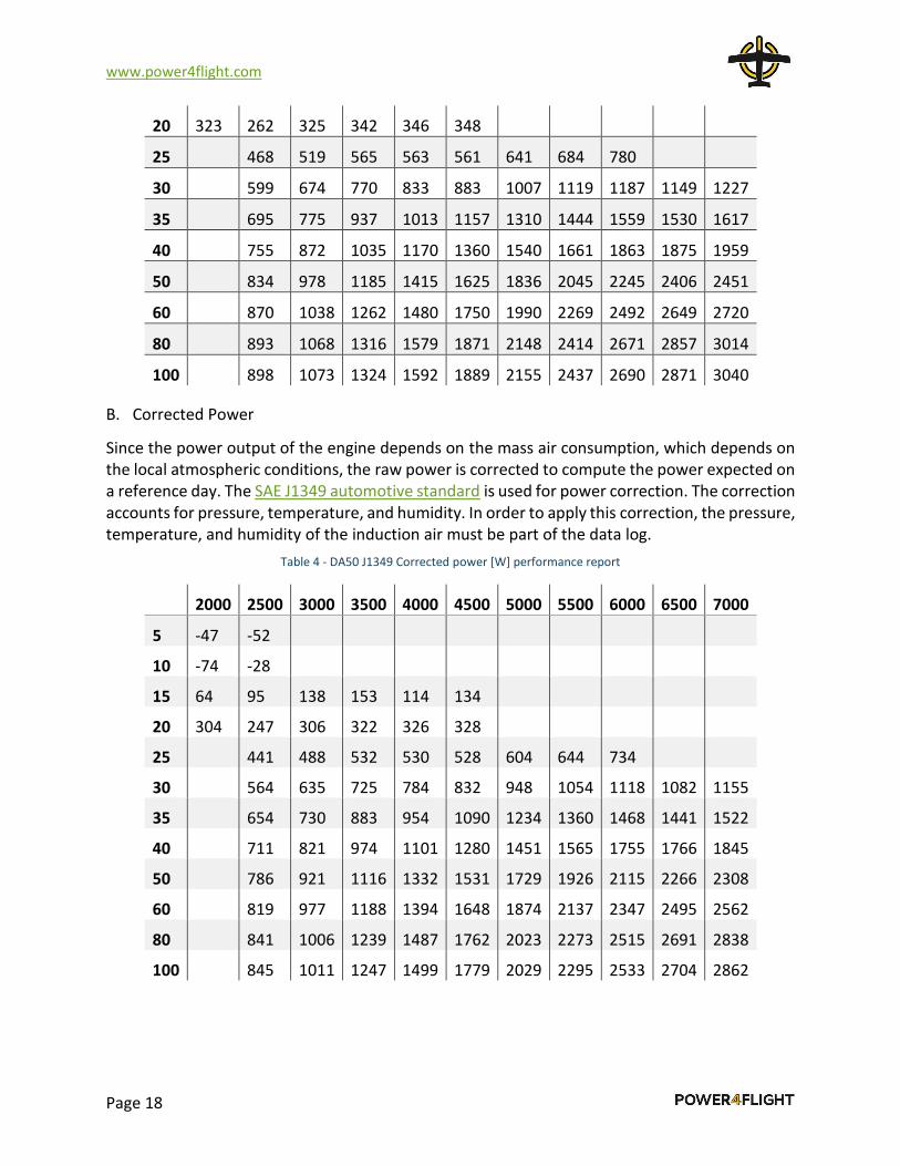
B. Corrected Power

Since the power output of the engine depends on the mass air consumption, which depends on the local atmospheric conditions, the raw power is corrected to compute the power expected on a reference day. The SAE J1349 automotive standard is used for power correction. The correction accounts for pressure, temperature, and humidity. In order to apply this correction, the pressure, temperature, and humidity of the induction air must be part of the data log.

Table 4 - DA50 J1349 Corrected power [W] performance report

2000 2500 3000 3500 4000 4500 5000 5500 6000 6500 7000

5 -47 -52

10 -74 -28

15 64 95 138 153 114 134

20 304 247 306 322 326 328

25 441 488 532 530 528 604 644 734

30 564 635 725 784 832 948 1054 1118 1082 1155

35 654 730 883 954 1090 1234 1360 1468 1441 1522

40 711 821 974 1101 1280 1451 1565 1755 1766 1845

50 786 921 1116 1332 1531 1729 1926 2115 2266 2308

60 819 977 1188 1394 1648 1874 2137 2347 2495 2562

80 841 1006 1239 1487 1762 2023 2273 2515 2691 2838

100 845 1011 1247 1499 1779 2029 2295 2533 2704 2862


http://www.sae.org/certifiedpower/


Page 19

C. Fuel flow

Although pseudo SFC works well for purposes of auto-calibration, the performance report needs the actual fuel flow. The fuel flow logged while mapping the fuel table is invalid since the amount of time between fuel value changes is not adequate to make an accurate fuel flow measurement. However, during the ignition mapping the fuel value is constant, so the measurement is reliable. As with the raw power, changes in fuel value from the ignition data log to the actual map fuel value must be accounted for. Since fuel flow is proportional to fuel value (all else being equal) the ratio of fuel values is applied to the recorded fuel flow to get the fuel flow for the report. The report also provides the brake specific fuel consumption, which is computed by dividing the fuel flow by the raw power.

Table 5 - DA50 Fuel flow [g/min] performance report

2000 2500 3000 3500 4000 4500 5000 5500 6000 6500 7000

5 1.4 1.0

10 2.0 1.5

15 3.2 2.4 2.9 3.3 3.2 3.7

20 3.2 3.7 3.9 4.2 4.4 4.9

25 4.8 5.3 5.4 5.7 6.0 6.8 7.5 7.2

30 5.4 5.9 7.0 6.9 7.0 7.8 8.5 9.6 9.5 9.8

35 6.6 6.7 7.9 8.1 9.0 9.7 10.6 11.9 12.1 12.2

40 7.2 7.7 8.5 9.7 10.4 11.2 11.4 13.1 13.6 14.5

50 8.4 8.9 10.8 12.1 13.3 14.3 16.2 17.1 18.4 19.6

60 9.2 10.2 11.8 14.0 14.8 16.4 22.7 21.0 22.5 23.6

80 9.9 10.9 12.8 15.0 17.8 20.0 21.4 24.7 27.3 28.4

100 9.8 11.1 13.2 15.1 17.7 20.2 23.4 26.5 29.4 29.9

Table 6 - DA50 BSFC [g/kW-hr] performance report

2000 2500 3000 3500 4000 4500 5000 5500 6000 6500 7000

15 2998 1495 1260 1304 1677 1655

20 632 889 761 782 819 888

25 656 650 610 646 682 679 696 587

30 572 553 580 531 507 491 482 515 526 510

35 604 551 535 511 498 473 468 485 503 480



Page 20

40 606 559 526 530 486 464 437 449 461 472

50 642 581 578 547 520 497 506 485 488 511

60 675 625 595 601 539 526 639 537 540 553

80 704 652 617 605 607 592 565 590 608 600

100 696 659 635 605 596 599 611 627 653 626

XII. CHALLENGES TO AUTOMATIC ENGINE MAPPING

A. Engine cooling

Cylinder head temperature (CHT) strongly influences the effective charge density of a two-stroke engine. Therefore, in order to measure performance changes due to fuel or ignition changes the CHT must be controlled to a constant value, typically between 120⁰C and 180⁰C. The control computer software receives the head temperature from the ECU once per second. A linear trajectory PIF8 control loop is updated on each CHT measurement to determine a new fan speed command.

Assuming the cooling fan has enough performance the fan control logic can maintain the CHT very accurately through the “auto” function (Figure 10). Large changes in throttle or speed may lead to excursions in the head temperature of a few degrees. Prior to the development of the automatic cooling fan control the dyno operator would spend a significant amount of time managing the engine temperature. Operator inattention could lead to poor calibrations or engine damage. Implementing the automatic cooling fan control was a necessary first step to automatic engine mapping; but it is also enormously useful for the human operator.

Figure 10 - Cooling fan control

B. Accounting for humidity

The ECU measures temperature and pressure and computes air density. In combination with the fuel value (VE) this estimates the mass of air consumed by the engine, and determines the amount of fuel by targeting a desired air to fuel ratio. It is implicit in the ECU logic that the mass flow of oxygen is a fixed fraction of the mass flow of air. However, the water vapor on a 100% humid standard day (15C, 101.3kPa) will displace nearly 3% of the oxygen. If the ECU is calibrated on a 100% humid standard day, then it will be using 3% less fuel than it should on a standard dry

8 A conventional PID loop could be used, but it would have significant overshoot when the operating condition changed. A more advanced design with trajectory shaping and feedforward from the throttle gives better results with less gain tuning.



Page 21

day. Since operating too lean is much more problematic than operating too rich the fuel value computed by the mapping algorithm must be artificially inflated to account for the extra oxygen that would appear on a dry day. From the J1349 Power correction standard the partial pressure of water vapor is:

𝑃𝑟𝑒𝑠𝑠𝑢𝑟𝑒𝐻2𝑂 = (𝑅𝐻

100) (

𝑒(77.345+0.0057∙𝑇−7235𝑇⁄ )

𝑇8.2)

Where:

PressureH2O is the partial pressure of water vapor in Pascals.

RH is the relative humidity of the air in percent.

T is the absolute temperature of the air in Kelvin.

Realistically a day drier than 20% relative humidity is unlikely to happen, so it is sufficient to consider the difference in oxygen from the mapping conditions to a 20% day at the same pressure and temperature. When the humidity of the air during mapping is greater than 20% a humidity corrected VE is computed as:

𝑉𝐸𝐶𝑂𝑅 = 𝑉𝐸𝑃𝑟𝑒𝑠𝑠𝑢𝑟𝑒

𝑃𝑟𝑒𝑠𝑠𝑢𝑟𝑒 − (𝑃𝑟𝑒𝑠𝑠𝑢𝑟𝑒𝐻2𝑂 − 𝑃𝑟𝑒𝑠𝑠𝑢𝑟𝑒𝐻2𝑂−20%)

Where:

VECOR is the humidity corrected VE

VE is the VE determined by the automatic mapping algorithm

Pressure is the air pressure in Pascals

PressureH2O is the partial pressure of water vapor in Pascals, computed from the humidity and temperature of the air.

PressureH2O-20% is the partial pressure of water vapor in Pascals, at the current air temperature and a humidity of 20%.

C. Handling faults

Since the goal of the automatic mapping system is to reduce human involvement the system must attract the attention of an operator when there is a problem. An alarm system was put in place which can alert the operator if data indicate there is a problem. The system can even shut down the dyno, engine, and fuel pump if the problem becomes critical.

Figure 11 shows the user interface for the alarm panel. The RPM mismatch, Dyno temp critical, and CHT critical alarms can affect a shutown. RPM mismatch is triggered if the RPM reported by the ECU and the RPM reported by the dyno do not agree - as in the case of a broken crankshaft.



Page 22

Figure 11 - User interface for the alarm panel


Automatic Fuel Injection Mapping for Small Two-Stroke Engines. · Whereas four-stroke engines have...

Documents

Transcript of Automatic Fuel Injection Mapping for Small Two-Stroke Engines. · Whereas four-stroke engines have...