
Automatic Feature Construction for Supervised ... · Orange Labs Automatic Feature Construction for...
77
Orange Labs Automatic Feature Construction for Supervised Classification from Large Scale Multi-Relational Data Marc Boullé, Orange Labs September 5, 2017 ILP 2017 27th International Conference on Inductive Logic Programming 4-6 Sep 2017 Orléans (France)
Transcript of Automatic Feature Construction for Supervised ... · Orange Labs Automatic Feature Construction for...

Orange Labs
Automatic Feature Construction
for Supervised Classification from Large Scale Multi-Relational Data
Marc Boullé, Orange Labs September 5, 2017
ILP 2017 27th International Conference on Inductive Logic Programming 4-6 Sep 2017 Orléans (France)

2
Orange today
Orange is one of the topmost European and African operators for mobile and broadband internet services as well as a world leader in providing telecommunication services to businesses.
Over 263 millions customers worldwide
The Group provides services for residential customers in 30 countries and for business customers in 220 countries and territories.

Orange Labs 3
Marketing campaigns Objective: scoring
• churn, appetency, up-selling…
Millions of instances
Multiple tables source data • Customer contracts
• Call detail records (billions)
• Multi-channel customer support
• External data
• …
Train sample • 100 000 instances
• 10 000 variables (based on expertise)
• Heavily unbalanced
• Missing values
• Thousands of categorical values
• …
Challenge: industrial scale • Hundred of scores every month
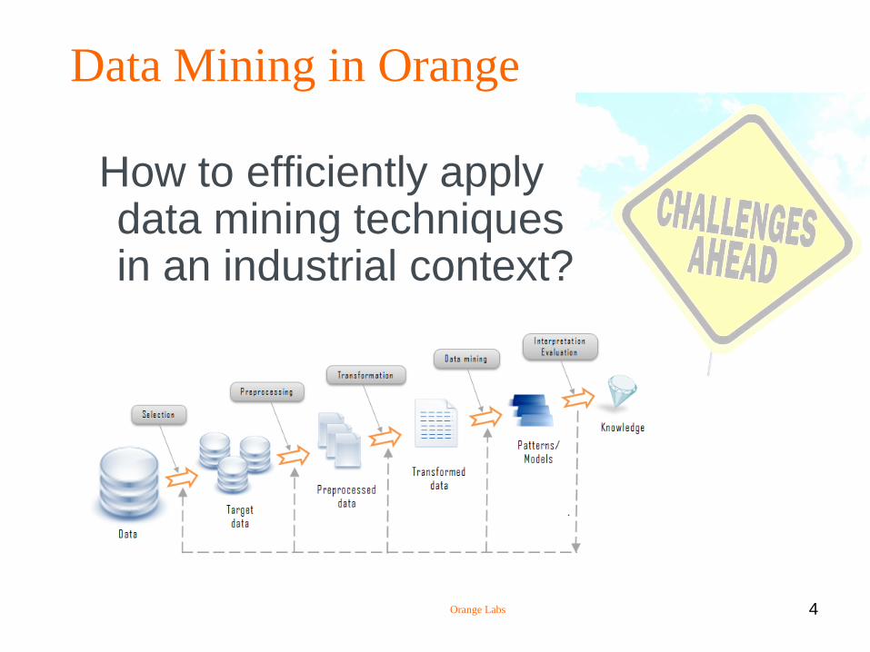
Data Mining in Orange Example of use case
Orange Labs 4
How to efficiently apply data mining techniques in an industrial context?
Data Mining in Orange
Orange Labs 5
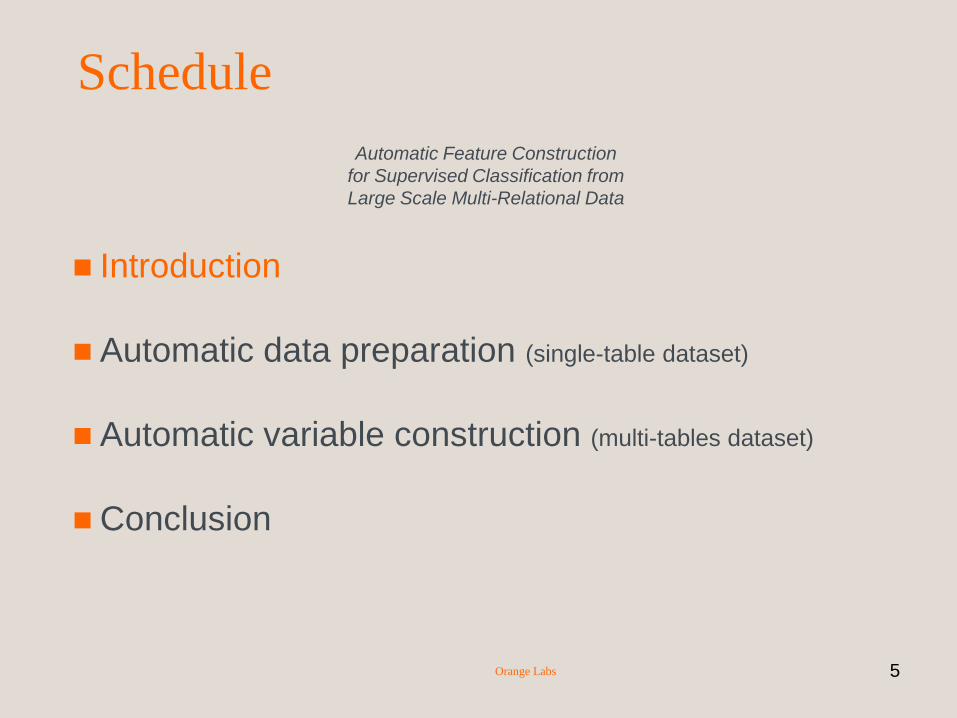
Automatic Feature Construction
for Supervised Classification from
Large Scale Multi-Relational Data
Introduction
Automatic data preparation (single-table dataset)
Automatic variable construction (multi-tables dataset)
Conclusion
Schedule

Orange Labs 6
Data Mining under Limited Resources
Data Mining in Industrial Context Applicable in a large variety of contexts
Vast demand but slow dissemination
Resource Disk space: fast growth
RAM: medium growth
CPU: medium growth
Skilled data analysts: steady
The lack of data analysts is the lock to the wide dissemination of the data mining solutions in business
lack of data analysts => Automatize !

Orange Labs 7
Many domains Marketing
Text mining
Web mining
Traffic classification
Sociology
Ergonomics
Many scales Tens to millions of instances
Up to billions of secondary records
Tens to hundreds of thousands of variables
Many types of data Numerical
Categorical
Text
Image
Relational databases
Many tasks Data exploration
Supervised
Unsupervised
Data Mining in Orange A wide variety of contexts
Data constraints Heterogeneous
Missing values
Categorical data with many values
Multiple classes
Heavily unbalanced distributions
Training requirements Fast data preparation and modeling
Model requirements Reliable
Accurate
Parsimonious (few variables)
Understandable
Deployment requirement Fast deployment
Up to real time classification in network devices
Business requirement Return of investment for the whole process
very large variety of contexts => Genericity
Orange Labs
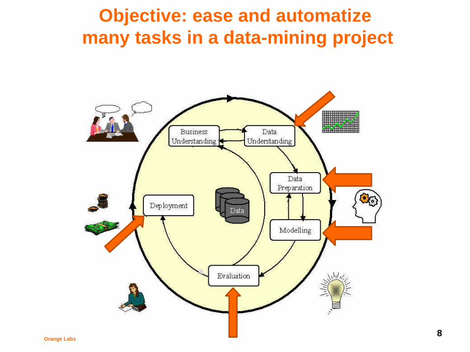
Objective: ease and automatize
many tasks in a data-mining project
8
Orange Labs 9
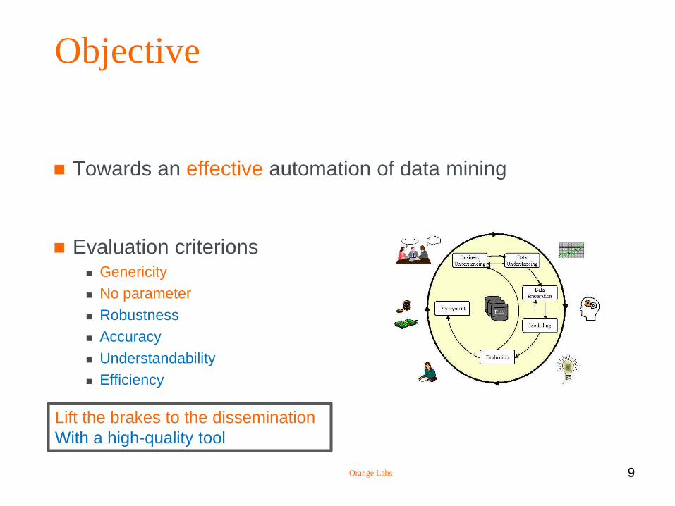
Objective
Towards an effective automation of data mining
Evaluation criterions Genericity
No parameter
Robustness
Accuracy
Understandability
Efficiency
Lift the brakes to the dissemination
With a high-quality tool

Orange Labs 10
Related work
Multi-table relational data mining Inductive logic programming
• uniform representation for examples, background knowledge and hypotheses
• formal logic rather than database oriented
Propositionalisation • build a flat instance x variable table from relational data
• use of a pattern language (aka declarative bias) to limit the expressiveness
Our approach Closely related to propositionalisation (aka feature construction)
Introduction of a probabilistic bias • Simple to use by the data analyst
• One single parameter: number of features to construct
• Resilient to over-fitting
• Scalable
Evaluation criterions Genericity
No parameter
Robustness
Accuracy
Understandability
Efficiency

Orange Labs 11
Automatic Feature Construction
for Supervised Classification from
Large Scale Multi-Relational Data
Introduction
Automatic data preparation (single-table dataset)
Automatic variable construction (multi-tables dataset)
Conclusion
Schedule

Orange Labs 12
Context
Statistical learning
Objective: train a model
• Classification: the output variable is categorical
• Regression: the output variable is numerical
• Clustering: no output variable
Data preparation
Variable selection
Search for a data representation
Data preparation is critical
80% of the process time
Requires skilled data analysts

Orange Labs 13
Single-table datasets instances x variables
Age Education Education
Num Marital status Occupation Race Sex
Hours
Per week
Native
country … Class
39 Bachelors 13 Never-married Adm-clerical White Male 40 United-States … less
50 Bachelors 13 Married-civ-spouse Exec-managerial White Male 13 United-States … less
38 HS-grad 9 Divorced Handlers-cleaners White Male 40 United-States … less
53 11th 7 Married-civ-spouse Handlers-cleaners Black Male 40 United-States … less
28 Bachelors 13 Married-civ-spouse Prof-specialty Black Female 40 Cuba … less
37 Masters 14 Married-civ-spouse Exec-managerial White Female 40 United-States … less
49 9th 5 Married-spouse-absent Other-service Black Female 16 Jamaica … less
52 HS-grad 9 Married-civ-spouse Exec-managerial White Male 45 United-States … more
31 Masters 14 Never-married Prof-specialty White Female 50 United-States … more
42 Bachelors 13 Married-civ-spouse Exec-managerial White Male 40 United-States … more
37 Some-college 10 Married-civ-spouse Exec-managerial Black Male 80 United-States … more
30 Bachelors 13 Married-civ-spouse Prof-specialty Asian Male 40 India … more
23 Bachelors 13 Never-married Adm-clerical White Female 30 United-States … less
32 Assoc-acdm 12 Never-married Sales Black Male 50 United-States … less
… … … … … … … … … … …

Orange Labs 14
Proposed approach: data grid models
Objective Evaluate the informativeness of variables
Data grid models for non parametric density estimation
Discretization of numerical variables
Value grouping of categorical variables
Data grid are the cross-product of the univariate partitions,
with a piecewise constant density estimation in each cell of the grid
Modeling approach: MODL Bayesian approach for model selection
• Minimum Description Length
Efficient optimization algorithms

Orange Labs 15
Data grid models for statistical analysis of a data table
Univariate Bivariate Multivariate
Classification
Y categorical P(Y | X) P(Y | X1, X2) P(Y | X1, X2 ,… , XK)
Regression
Y numerical P(Y | X) P(Y | X1, X2) P(Y | X1, X2 ,… , XK)
Coclustering _
P(Y1, Y2) P(Y1, Y2 ,… ,YK)
Output variables (Y) or input variables (X)
Numerical or categorical variables
From univariate to multivariate
Supervised learning: conditional density estimation
Unsupervised learning: joint density estimation

Orange Labs 16
Classification Discretization of numerical variables
Univariate analysis
Numerical input variable X
Categorical output variable Y
Discretization for univariate conditional density estimation
Univariate Bivariate Multivariate
Classification
Y categorical P(Y | X) P(Y | X1, X2) P(Y | X1, X2 ,… , XK)
Regression
Y numerical P(Y | X) P(Y | X1, X2) P(Y | X1, X2 ,… , XK)
Clustering _
P(Y1, Y2) P(Y1, Y2 ,… , YK)
Orange Labs 17
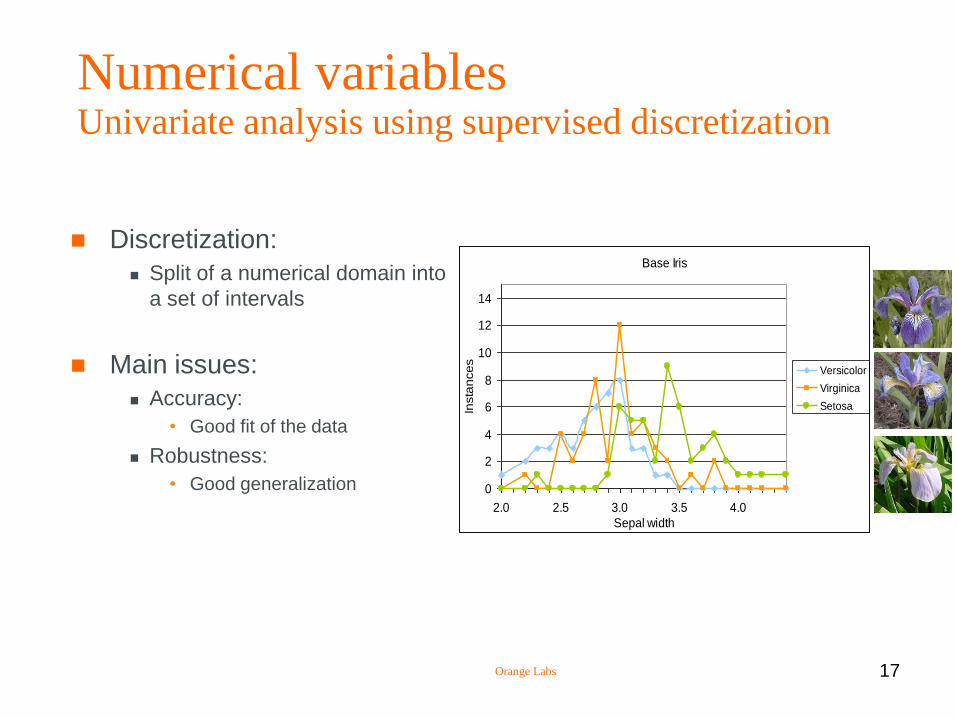
Numerical variables Univariate analysis using supervised discretization
Discretization:
Split of a numerical domain into
a set of intervals
Main issues:
Accuracy:
• Good fit of the data
Robustness:
• Good generalization
Base Iris
0
2
4
6
8
10
12
14
2.0 2.5 3.0 3.5 4.0
Sepal width
Insta
nce
s
Versicolor
Virginica
Setosa

Orange Labs 18
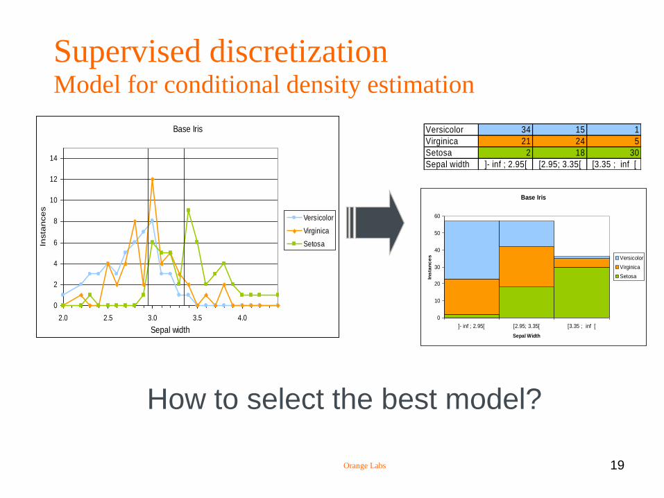
Supervised discretization Model for conditional density estimation
Versicolor 34 15 1
Virginica 21 24 5
Setosa 2 18 30
Sepal width ]- inf ; 2.95[ [2.95; 3.35[ [3.35 ; inf [
Base Iris
0
10
20
30
40
50
60
]- inf ; 2.95[ [2.95; 3.35[ [3.35 ; inf [
Sepal Width
Ins
tan
ce
s Versicolor
Virginica
Setosa
Base Iris
0
2
4
6
8
10
12
14
2.0 2.5 3.0 3.5 4.0
Sepal width
Insta
nce
s
Versicolor
Virginica
Setosa
Orange Labs 19
Supervised discretization Model for conditional density estimation
Versicolor 34 15 1
Virginica 21 24 5
Setosa 2 18 30
Sepal width ]- inf ; 2.95[ [2.95; 3.35[ [3.35 ; inf [
Base Iris
0
10
20
30
40
50
60
]- inf ; 2.95[ [2.95; 3.35[ [3.35 ; inf [
Sepal Width
Ins
tan
ce
s Versicolor
Virginica
Setosa
Base Iris
0
2
4
6
8
10
12
14
2.0 2.5 3.0 3.5 4.0
Sepal width
Insta
nce
s
Versicolor
Virginica
Setosa
How to select the best model?

Orange Labs 20
Formalization
Definition: A discretization model is defined by:
the number of input intervals,
the partition of the input variable into intervals,
the distribution of the output values in each interval.

Orange Labs 21
Formalization
Definition: A discretization model is defined by:
the number of input intervals,
the partition of the input variable into intervals,
the distribution of the output values in each interval.
Notations:
N: number of instances
J: number of classes
I: number of intervals
Ni.: number of instances in the interval i
Nij: number of instances in the interval i for class j

Orange Labs 22
Bayesian approach for model selection
Best model: the most probable model given the data
Maximize
Using a decomposition of the model parameters
Assuming independence of the output distributions in each interval
We now need to evaluate the prior distribution of the model
parameters
||
P M P D MP M D
P D
| | | , |i ij iP M P D M P I P N I P N I N P D M
. .
1 1
| | | , |I I
i ij i i
i i
P M P D M P I P N I P N I N P D M

Orange Labs 23
Prior distribution of the models
Definition: We define the hierarchical prior as follows:
the number of intervals is uniformly distributed between 1 et N,
for a given number of intervals I, every set of I interval bounds are
equiprobable,
for a given interval, every distribution of the output values are
equiprobable,
the distributions of the output values on each input interval are
independent from each other.
Hierarchical prior, uniformly distributed at each stage of the
hierarchy

Orange Labs 24
Optimal evaluation criterion MODL
Theorem: A discretization model distributed according the
hierarchical prior is Bayes optimal for a given set of
instances if the following criterion is minimal:
1° term: choice of the number of intervals
2° term: choice of the bounds of the intervals
3° term: choice of the output distribution Y in each interval
4° term: likelihood of the data given the model
.
. 1 2
1 1
1 1log log log log ! ! !... !
1 1
I Ii
i i i iJ
i i
N I N JN N N N N
I J
likelihood prior N: number of instances
J: number of classes
I: number of intervals
Ni.: number of instances in the interval i
Nij: number of instances in the interval i for class j

Orange Labs 25
Discretization algorithm Quasi-optimal heuristic
Optimal solution in O(N 3)
Based on dynamic programing
Usefull to evaluate the quality of optimization heuristics
Approximated solution in O(N log(N))
Greedy bottom-up heuristic
Post-optimisations to improve the solution • split interval, merge interval, move interval boundary
Evaluation on 2000 discretizations Optimal solution in more than 95% of the cases
In the remaining 5%, solution close from the optimal one (diff<0.15%)
Discretization intervals
… Ik-1 Ik Ik+1 Ik+2 Ik+3 …
Split of interval Ik
Merge of interval Ik and Ik+1
Merge-Split of intervals Ik and Ik+1
Merge-Merge-Split of intervals Ik, Ik+1 and Ik+2

Orange Labs 26
Classification Discretization of numerical variables
Evaluation
Orange Labs 27
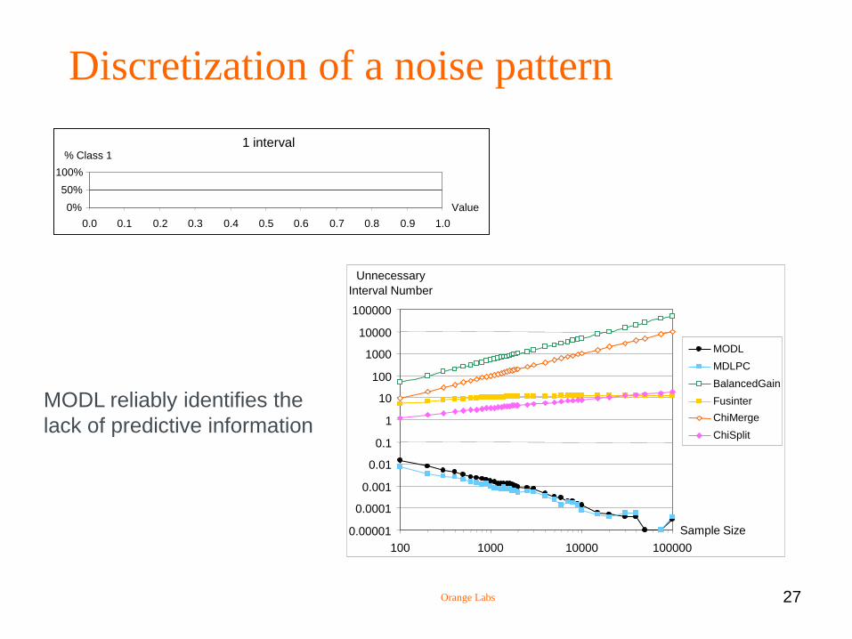
Discretization of a noise pattern
MODL reliably identifies the
lack of predictive information
1 interval
0%
50%
100%
0.0 0.1 0.2 0.3 0.4 0.5 0.6 0.7 0.8 0.9 1.0
Value
% Class 1
0.00001
0.0001
0.001
0.01
0.1
1
10
100
1000
10000
100000
100 1000 10000 100000
Sample Size
Unnecessary
Interval Number
MODL
MDLPC
BalancedGain
Fusinter
ChiMerge
ChiSplit

Orange Labs 28
Discretization of a crenel pattern
MODL correctly identifies the
relevant information with a
minimal number of instances
100 intervals
0%
50%
100%
0.0 0.1 0.2 0.3 0.4 0.5 0.6 0.7 0.8 0.9 1.0
Value
% Class 1
1
10
100
1000
10000
100 1000 10000 100000
Sample Size
Interval Number
MODL
MDLPC
BalancedGain
Fusinter
ChiMerge
ChiSplit

Orange Labs 29
Classification Value grouping of categorical variables
Univariate analysis
Categorical input variable X
Categorical output variable Y
Value grouping for univariate conditional density estimation
Univariate Bivariate Multivariate
Classification
Y categorical P(Y | X) P(Y | X1, X2) P(Y | X1, X2 ,… , XK)
Regression
Y numerical P(Y | X) P(Y | X1, X2) P(Y | X1, X2 ,… , XK)
Coclustering _
P(Y1, Y2) P(Y1, Y2 ,… , YK)

Orange Labs 30
Categorical variables Univariate analysis using value grouping
Cap color EDIBLE POISONOUS Frequency
BROWN 55.2% 44.8% 1610
GRAY 61.2% 38.8% 1458
RED 40.2% 59.8% 1066
YELLOW 38.4% 61.6% 743
WHITE 69.9% 30.1% 711
BUFF 30.3% 69.7% 122
PINK 39.6% 60.4% 101
CINNAMON 71.0% 29.0% 31
GREEN 100.0% 0.0% 13
PURPLE 100.0% 0.0% 10
RED
YELLOW
BUFF
PINK
BROWN
GRAY
GREEN
PURPLEWHITE
CINNAMON
G_RED G_BROWN
G_GRAY
G_GREENG_WHITE
Cap color EDIBLE POISONOUS Frequency
G_RED 38.9% 61.1% 2032
G_BROWN 55.2% 44.8% 1610
G_GRAY 61.2% 38.8% 1458
G_WHITE 69.9% 30.1% 742
G_GREEN 100.0% 0.0% 23

Orange Labs 31
Categorical variables Univariate analysis using value grouping
Cap color EDIBLE POISONOUS Frequency
BROWN 55.2% 44.8% 1610
GRAY 61.2% 38.8% 1458
RED 40.2% 59.8% 1066
YELLOW 38.4% 61.6% 743
WHITE 69.9% 30.1% 711
BUFF 30.3% 69.7% 122
PINK 39.6% 60.4% 101
CINNAMON 71.0% 29.0% 31
GREEN 100.0% 0.0% 13
PURPLE 100.0% 0.0% 10
RED
YELLOW
BUFF
PINK
BROWN
GRAY
GREEN
PURPLEWHITE
CINNAMON
G_RED G_BROWN
G_GRAY
G_GREENG_WHITE
Cap color EDIBLE POISONOUS Frequency
G_RED 38.9% 61.1% 2032
G_BROWN 55.2% 44.8% 1610
G_GRAY 61.2% 38.8% 1458
G_WHITE 69.9% 30.1% 742
G_GREEN 100.0% 0.0% 23
How to select the best model?
Orange Labs 32
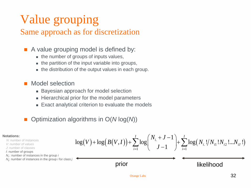
Value grouping Same approach as for discretization
A value grouping model is defined by: the number of groups of inputs values,
the partition of the input variable into groups,
the distribution of the output values in each group.
Model selection Bayesian approach for model selection
Hierarchical prior for the model parameters
Exact analytical criterion to evaluate the models
Optimization algorithms in O(N log(N))
.
. 1 2
1 1
1log log , log log ! ! !... !
1
I Ii
i i i iJ
i i
N JV B V I N N N N
J
likelihood prior
Notations:
N: number of instances
V: number of values
J: number of classes
I: number of groups
Ni.: number of instances in the group i
Nij: number of instances in the group i for class j

Orange Labs 33
Classification Bivariate discretization of numerical variables
Bivariate analysis
Numerical input variables X1 and X2
Categorical output variable Y
Bivariate discretization for bivariate conditional density estimation
Univariate Bivariate Multivariate
Classification
Y categorical P(Y | X) P(Y | X1, X2) P(Y | X1, X2 ,… , XK)
Regression
Y numerical P(Y | X) P(Y | X1, X2) P(Y | X1, X2 ,… , XK)
Clustering _
P(Y1, Y2) P(Y1, Y2 ,… , YK)

Orange Labs 34
Pair of numerical variables
Wine
0
1
2
3
4
5
6
11 12 13 14 15
V1
V7
Class 1
Class 2
Class 3

Orange Labs 35
Pair of numerical variables Bivariate discretization as a conditional density estimator
]2.18;+inf[ (0, 23, 0) (59, 0, 4)
]1.235;2.18] (0, 35, 0) (0, 5, 6)
]-inf;1.235] (0, 4, 11) (0, 0, 31)
V7xV1 ]-inf;12.78] ]12.78;+inf[
Wine
0
1
2
3
4
5
6
11 12 13 14 15
V1
V7
Class 1
Class 2
Class 3
Each input variable is discretized
We obtain a bivariate data grid
In each cell, the conditional
density is estimated by counting

Orange Labs 36
Application of the MODL approach
Explicit formalization of the model family
Definition of the model parameters
Definition of a prior distribution on the parameters of the
bivariate discretization models
Hierarchical prior
Uniform distribution at each stage of the hierarchy
We obtain an exact analytical evaluation criterion
1 2 1 21 2 .. . ., , , ,i i i i jI I N N N
1 2
1 2
1 2
1 2
1 2 1 2 1 2 1 2
1 2
.1 2
1 11 2
. 1 2
1 1
11 1log log log log log
1 1 1
log ! ! !... !
I Ii i
i i
I I
i i i i i i i i J
i i
N JN I N IN N
I I J
N N N N
likelihood
prior

Orange Labs 37
Classification Bivariate discretization of numerical variables
Evaluation
Orange Labs 38
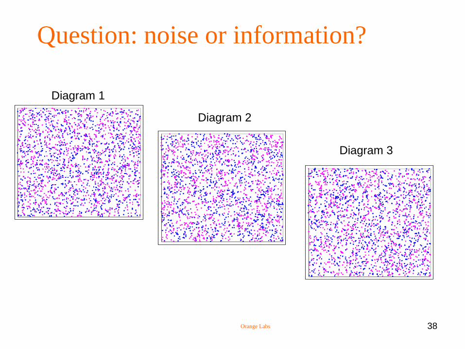
Question: noise or information?
Diagram 1
Diagram 2
Diagram 3

Orange Labs 39
Diagram 1 noise
Diagram 1 (2000 points) Data grid 1 x 1 (1 cell)
Value of criterion = 2075

Orange Labs 40
Diagram 2 chessboard 8 x 8 with 25% noise
Diagram 2 (2000 points) Data grid 8 x 8 (64 cells)
Value of criterion = 1900
Orange Labs 41
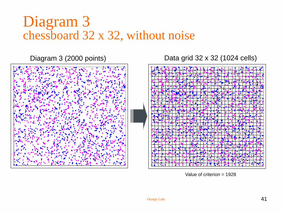
Diagram 3 chessboard 32 x 32, without noise
Diagram 3 (2000 points) Data grid 32 x 32 (1024 cells)
Value of criterion = 1928
Orange Labs 42
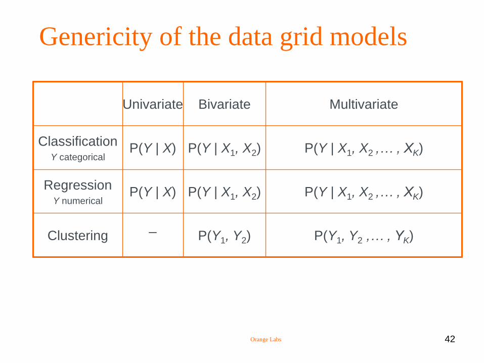
Genericity of the data grid models
Univariate Bivariate Multivariate
Classification Y categorical
P(Y | X) P(Y | X1, X2) P(Y | X1, X2 ,… , XK)
Regression Y numerical
P(Y | X) P(Y | X1, X2) P(Y | X1, X2 ,… , XK)
Clustering _
P(Y1, Y2) P(Y1, Y2 ,… , YK)
Orange Labs 43
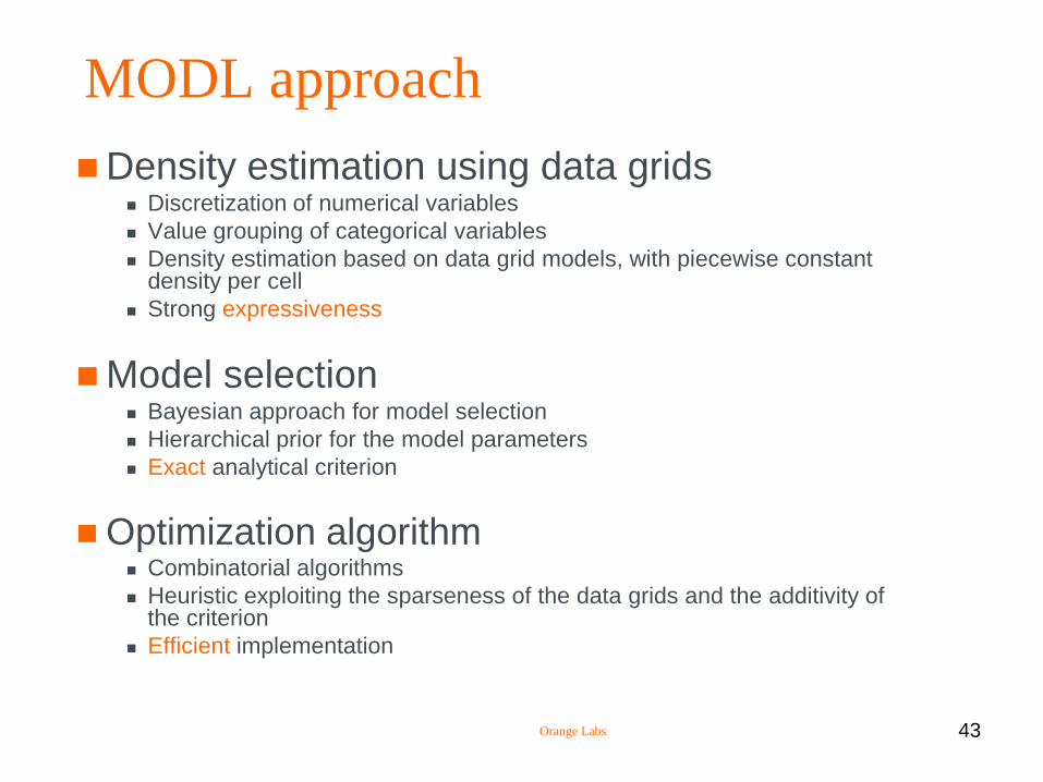
MODL approach
Density estimation using data grids Discretization of numerical variables
Value grouping of categorical variables
Density estimation based on data grid models, with piecewise constant density per cell
Strong expressiveness
Model selection Bayesian approach for model selection
Hierarchical prior for the model parameters
Exact analytical criterion
Optimization algorithm Combinatorial algorithms
Heuristic exploiting the sparseness of the data grids and the additivity of the criterion
Efficient implementation

Orange Labs 44
MODL approach Towards an automatisation of data preparation
Data preparation Recoding
Evaluation of conditional or joint density
Variable selection
• Variables can be sorted by decreasing informativeness
Advantages of the MODL approach Genericity
Parameter-free
Reliability
Accuracy
Interpretability
Efficiency

Orange Labs 45
Automatic Feature Construction
for Supervised Classification from
Large Scale Multi-Relational Data
Introduction
Automatic data preparation (single-table dataset)
Automatic variable construction (multi-tables dataset)
Conclusion
Schedule

Orange Labs 46
Where does data come from?
Data
Sources
More
Data
Less
Data
Historized
Normalized
Detailed
Customer Behavior
Usa
ge P
rofi
le
Mig
rati
on
in
Usa
ge
Lo
ya
lty &
Sw
itch
ing
Customer Interactions
Ac
qu
isit
ion
Info
rma
tio
n
Inb
ou
nd
Co
nta
ct
Ou
tbo
un
d C
on
tac
t
Cam
paig
n H
isto
ry
Customer Profile
Dem
og
rap
hic
s &
Fir
mg
rap
hic
s
Att
itu
des
Pro
du
ct
& S
erv
ice
Pre
fere
nce
s
External
Data
Ge
o-
dem
og
rap
hic
s
Cen
su
s
Data
Warehouse
Data Marts
Inputs target

Orange Labs
Big Data = relational data!
Fact Table
Dimension
Table (log)
0:N
ID; Target
47

Orange Labs
Big Data = relational data!
Generalization
Star Schema
Snowflake Schema
More complex structures are
not considered (Yet):
Fact Table
Dimension
Table (log)
0:N
ID; Target
48

Orange Labs
Big Data = relational data!
Flattening Such a Relational Structure leads to
an Infinite Flat table
Fact Table
Dimension
Table (log)
0:N
ID Target
? The data
"explanatory"
(potentially)
1
0
…
1
Variables Target
Insta
nce
s
49
Orange Labs
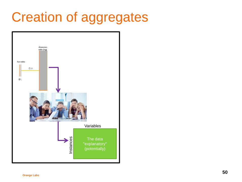
Creation of aggregates
The data
"explanatory"
(potentially)
Variables
Insta
nce
s
50

Orange Labs
Creation of aggregates
• Long • Time expensive process to get a flat table
usable for data analysis
• Costly • Expert knowledge necessary to constructed
new variables
• Risky • Risk of missing informative variables
• Risk of constructing and selecting irrelevant
variables
• Data-mart specified once for all from
business knowledge from a History …
• … and it is hoped valid for a whole
range of Future problems
• (a little caricature, the specification of the data mart evolves
in the course of the time but always a posteriori) The data
"explanatory"
(potentially)
Variables
Insta
nce
s
51

Orange Labs 52
Automatic variable construction
Search for an efficient data representation Context: supervised analysis
• especially, in the multi-tables settings
Data preparation: • automatic variable selection
• next step: automatic variable construction (propositionalisation)
Objective: Explore numerous data representations using variable construction
Select the best representation
Challenges The number of constructed variables is infinite
• it is a subset of all computer programs
How to specify domain knowledge in order to control the space of constructed variables?
How to efficiently exploit this domain knowledge in order to reach the objective?
• Explore a very large search space
• Prevent the risk of over-fitting

Orange Labs 53
Automatic Feature Construction
for Supervised Classification from
Large Scale Multi-Relational Data
Introduction
Automatic data preparation (single-table dataset)
Automatic variable construction (multi-tables dataset)
Specification of domain knowledge
Evaluation of constructed variables
Sampling a subset of constructed variables
Experiments
Conclusion
Schedule

Orange Labs 54
Specification of data format
Table Two kinds of tables
• Root table: statistical unit of the studied problem
• Secondary table: sub-part of the statistical unit
Variables of simple type • Numerical (Num)
• Categorical (Cat)
Variables of advanced type • Date, Time, Timestamp…
Variables of relation type • Simple composition: sub-entity with 0-1 relation (Entity)
• Multiple composition: sub-entity with 0-n relation (Table)
Multi-table format
Customer
#id_customer: Cat
Name: Cat
Age: Num
Usages: Table(Usage)
MainAddress: Entity(Address)
Class: Cat
Usage
#id_customer: Cat
Product: Cat
useDate: Date
Address
#id_customer: Cat
StreetNumber: Num
StreetName: Cat
City: Cat

Orange Labs 55
Specification of a variable construction language
Construction rule Program function
• Input: one or several values • Output: one value
Type of values • Simple: Numerical, Categorical • Advanced: Date, Time, Timestamp… • Relation: Entity or Table
Constructed variable Output of a construction rule
Rule operands
• Value • Variable • Output of another rule
Examples: New variables constructed in table Customer
• MainProduct = Mode(Usages, Product)
• LastUsageYearDay = Max(Usages, YearDay(useDate))
• NbUsageProd1FirstQuarter = Count(Selection(Usages, YearDay(useDate) in [1 ;90] and Product = “Prod1”))
• …
Customer
#id_customer: Cat
Name: Cat
Class: Cat
MainProduct: Cat
LastUsageYearDay: Num
NbUsageProd1FirstQuarter: Num
...
Multi-table format
Tabular format (instances*variables)
Variable construction (in memory)
Customer
#id_customer: Cat
Name: Cat
Age: Num
Usages: Table(Usage)
MainAddress: Entity(Address)
Class: Cat
Usage
#id_customer: Cat
Product: Cat
useDate: Date
Address
#id_customer: Cat
StreetNumber: Num
StreetName: Cat
City: Cat

Orange Labs 56
Variable construction language List of construction rules
Name Return type Operands Label
Count Num Table Number of records in a table
CountDistinct Num Table, Cat Number of distinct values
Mode Cat Table, Cat Most frequent value
Mean Num Table, Num Mean value
StdDev Num Table, Num Standard deviation
Median Num Table, Num Median value
Min Num Table, Num Min value
Max Num Table, Num Max value
Sum Num Table, Num Sum of values
Selection Table Table, (Cat, Num…) Selection from a table given a selection criterion
YearDay Num Date Day in year
WeekDay Num Date Day in week
DecimalTime Num Time Decimal hour in day
… … … …

Orange Labs 57
Towards automatic variable construction, data preparation and modeling for large scale multi-tables datasets
Introduction
Automatic data preparation (single-table dataset)
Automatic variable construction (multi-tables dataset)
Specification of domain knowledge
Evaluation of constructed variables
Sampling a subset of constructed variables
Experiments
Conclusion
Schedule
Orange Labs 58
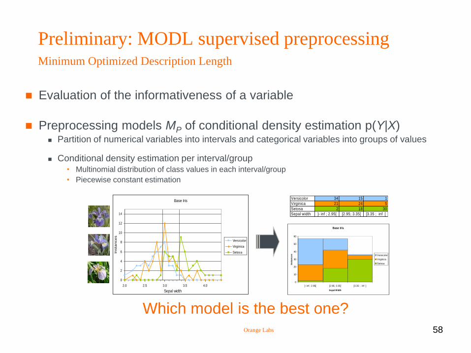
Preliminary: MODL supervised preprocessing Minimum Optimized Description Length
Evaluation of the informativeness of a variable
Preprocessing models MP of conditional density estimation p(Y|X) Partition of numerical variables into intervals and categorical variables into groups of values
Conditional density estimation per interval/group • Multinomial distribution of class values in each interval/group
• Piecewise constant estimation
Versicolor 34 15 1
Virginica 21 24 5
Setosa 2 18 30
Sepal width ]- inf ; 2.95[ [2.95; 3.35[ [3.35 ; inf [
Base Iris
0
10
20
30
40
50
60
]- inf ; 2.95[ [2.95; 3.35[ [3.35 ; inf [
Sepal WidthIn
sta
nc
es Versicolor
Virginica
Setosa
Base Iris
0
2
4
6
8
10
12
14
2.0 2.5 3.0 3.5 4.0
Sepal width
Insta
nce
s
Versicolor
Virginica
Setosa
Which model is the best one?

Orange Labs 59
MODL approach: evaluation of one variable Posterior probability of a preprocessing model
Prior distribution of parameters of model MP Bayesian approach MAP (maximum a posteriori)
• Hierarchical prior
• Uniform at each stage of the parameter hierarchy
Crude MDL approach • Negative log of the prior probability and of the likelihood
• Basic coding based of counting the number of possible parameterizations
Evaluation criterion Exact analytical formula
Regularized conditional entropy estimator
Null model and variable filtering Null model: coding the target variable directly
Variables with cost beyond the null cost are filtered to prevent over-fitting
Evaluation of a variable: compression rate
| ,P Y P Xc X L M X L D M X D
|c X N Ent Y X
* | ,P Y P Xp M X p D M X D
Penalization of complex preprocessing models
c N Ent Y
( ) 1Level X c X c

Orange Labs 60
MODL approach: construction of one variable
Definition of modeling space MC of constructed variables Exploit the domain knowledge
Exploit the multi-table format of the input data
A constructed variable X is a formula
• it is a « small » computer program
Definition of a prior distribution on all constructed variables
Evaluation criterion of a constructed variable
| ,C P Y P Xc X L M X L M X L D M X D
logC CL M X p M X
Penalization of complex constructed variables

Orange Labs 61
Prior distribution on all constructed variables Example
Rules YearDay Weekday Mode Min Max
Cost of Name L(MC(X)) = log(3) Choice of variable : log(3)
Cost of Min(Usages, YearDay(Date)) L(MC(X)) = log(3)+log(3)+log(1)+log(1)+log(2)+log(1) Choice of constructing a variable: log(3) Choice of rule Min: log(3) Choice of first operand (Usages) of Min: log(1) Choice of constructing a variable for second operand of Min: log(1) Choice of rule YearDay: log(2) Choice of operand of YearDay (Date): log(1)
Native/
Constructed
Name
Age
Choice of rule
Mode Usages Product
Min Usages
YearDay Date
WeekDay Date
Max Usages
YearDay Date
WeekDay Date
Customer
#id_customer: Cat
Name: Cat
Age: Num
Usages: OA(Usage)
Address: O(Address)
Class: Cat
Usage
#id_customer: Cat
Product: Cat
useDate: Date
Address
#id_customer: Cat
StreetNumber: Num
StreetName: Cat
City: Cat
Hierarchy of Multinomial Distributions with potentially Infinite Depth (HMDID) prior
Orange Labs 62
Automatic Feature Construction
for Supervised Classification from
Large Scale Multi-Relational Data
Introduction
Automatic data preparation (single-table dataset)
Automatic variable construction (multi-tables dataset)
Specification of domain knowledge
Evaluation of constructed variables
Sampling a subset of constructed variables
Experiments
Conclusion
Schedule

Orange Labs 63
Exploitation of domain knowledge How to draw a sample from the space of variable construction?
Objective: draw a sample of K variables At this step, the problem of selecting the informative variables is ignored
Principle Draw the variables one by one according to the HMDID prior
Naive algorithm: successive random draws Input: K {Number of draws}
Sortie: X={X} ,|X|≤K {Sample of constructed variables}
• 1: X=Ø
• 2: for k = 1 to K do
• 3: Draw X according to HMDID prior
• 4: Add X into X
• 5: end for Native/
Constructed
Name
Age
Choice of rule
TableMode Usages Product
TableMin Usages
YearDay Date
WeekDay Date
TableMax Usages
YearDay Date
WeekDay Date

Orange Labs 64
Exploitation of domain knowledge The naive algorithm is neither efficient not computable
The naive algorithm is not efficient Most draws do not produce new variables
Few constructed variables are drawn in case of numerous native variables
The naive algorithm is not computable Example:
• Variable v de type Num, rule f(Num, Num) -> Num
• Example: f = Sum(., .)
• Family of constructed variables
Catalan number Cn • Cn is the number of different ways n + 1 factors can be completely parenthesized
• Cn is also the number of full binary trees with n+1 leaves
Expectation of the size of formula: infinite
Size Example Coding Coding length Prior Number of variables
1 x 0 1 2-1 1
2 f(x,x) 100 3 2-3 1
3 f(f(x,x), x) 11000 5 2-5 2
4 f(f(x,f(x,x)), x) 1101000 7 2-7 5
5 f(f(x,f(x,x)), f(x,x)) 110100100 9 2-9 14
...
n 2n-1 2-(2n-1) C(n-1)
2 1
1
1
2n
n
n
E s X n C

Orange Labs 65
Exploitation of domain knowledge Draw many constructed variables simultaneously Principle
Draw directly a sample of variables according to prior HMDID
Exploit the multinomial maximum likelihood of the whole sample
Whole sample algorithm: simultaneous random draws Input: K {Number of draws}
Output: X={X} ,|X|≤K {Sample of constructed variables}
• 1: X=Ø
• 2: Start from root node of hierarchy of HMDID prior
• 3: Compute number of draws Ki per child node of the prior (native variable, rule, operand...)
• 4: for all child node in current node of the prior do
• 5: if leaf node of the prior (constructed variable with complete formula) then • 6: Add X into X
• 7: else
• 8: Propagate construction recursively by distributing the Ki draws
on each child node according to the multinomial distribution
• 9: end if
• 10: end for
The whole sample algorithm is both
efficient and computable
1 2
1 2
1 2
M L reached with frequencies
!...
! !... !Kn n n
K
K
k k
np D p p p
n n n
n p n
Native/
Constructed
Name
Age
Choice of rule
TableMode Usages Product
TableMin Usages
YearDay Date
WeekDay Date
TableMax Usages
YearDay Date
WeekDay Date

Orange Labs 66
Automatic Feature Construction
for Supervised Classification from
Large Scale Multi-Relational Data
Introduction
Automatic data preparation (single-table dataset)
Automatic variable construction (multi-tables dataset)
Specification of domain knowledge
Evaluation of constructed variables
Sampling a subset of constructed variables
Experiments
Conclusion
Schedule

Orange Labs 67
Benchmark Datasets
14 benchmark multi-tables datasets
Various domains
• Handwritten digit
• Pen tip trajectory character
• Australian sign language
• Image
• Speaker recognition
• Molecular chemistry
• Genomics
• …
Various sizes and complexity • 100 to 5000 instances
• 500 to 5000000 records in secondary tables
• Numerical and categorical variables
• 2 to 96 classes
• Unbalanced class distribution
Dataset Instances Records Cat. var Num. var Classes Maj.
Auslan 2565 146949 1 23 96 0.011
CharacterTrajectories 2858 487277 1 4 20 0.065
Diterpenes 1503 30060 2 1 23 0.298
JapaneseVowels 640 9961 1 13 9 0.184
MimlDesert 2000 18000 1 15 2 0.796
MimlMountains 2000 18000 1 15 2 0.771
MimlSea 2000 18000 1 15 2 0.71
MimlSunset 2000 18000 1 15 2 0.768
MimlTrees 2000 18000 1 15 2 0.72
Musk1 92 476 1 166 2 0.511
Musk2 102 6598 1 166 2 0.618
Mutagenesis 188 10136 3 4 2 0.665
OptDigits 5620 5754880 1 3 10 0.102
SpliceJunction 3178 191400 2 1 3 0.521

Orange Labs 68
Benchmark Evaluation protocol
Compared methods MODL: our method
• Construction rules: Selection, Count, Mode, CountDistinct, Mean, Median, Min, Max StdDev, Sum
• Preprocessing: supervised discretisation and value grouping
• Classifier: Selective Naive Bayes (variable selection and model averaging)
• Number of variables to construct: 1, 3, 10, 30, 10, 300, 1000, 3000, 10000
RELAGGS: (Krogel et al, 2001) • Construction rules: same as MODL (except Selection), plus Count per categorical value
• Preprocessing and classifier: same as MODL
1BC: (Lachiche et al, 1999) • first-order Bayesian classifier with preprositionalisation
• Preprocessing: equal frequency discretization with 1, 2, 5, 10, 20, 50, 100, 200 bins
1BC2: (Lachiche et al, 2002) • Successor of 1BC
• True first order classifier
Evaluation protocol Stratified 10-fold cross validation
Collected results: number of constructed variables and test accuracy

Orange Labs 69
Benchmark results Control of variable construction
RELAGGS, 1BC, 1BC2: No control on the number of constructed variables
MODL Exactly the requested number of constructed variables
Orange Labs 70
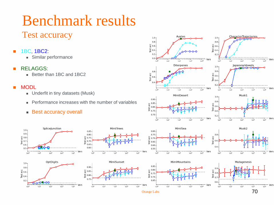
Benchmark results Test accuracy
1BC, 1BC2: Similar performance
RELAGGS: Better than 1BC and 1BC2
MODL
Underfit in tiny datasets (Musk)
Performance increases with the number of variables
Best accuracy overall

Orange Labs 71
Benchmark: robustness
Protocol
Random shuffle of class values in each dataset
Experiments repeated in 10 cross-validation
• 10000 constructed variables per dataset in each fold
• 1.4 million of variables evaluated overall
Results
With construction regularization
• Not one single wrongly selected variable, among the 1.4 million
• Highly robust approach
Orange Labs 72
Use cases in Orange Experiments on large datasets
100 000 customers • up to millions in main table
50 millions call detail records • up to billions in secondary tables
• up to hundreds of GB
Up to 100 000 automatically constructed variables
Results Genericiy
Parameter-free • Rely on domain knowledge description: multi-table specification and choice of construction rules
Reliability
Accuracy
Interpretability: • Constructed variables may be numerous, redundant and some of them complex
Efficicency
Use cases and methodology: needs to be invented Automatic evaluation of additional data sources
Fast automatic solution to many data mining problems
Help to suggest new variables to construct
…

Orange Labs 73
Towards automatic variable construction, data preparation and modeling
for large scale multi-tables datasets
Introduction
Automatic data preparation (single-table dataset)
Automatic variable construction (multi-tables dataset)
Conclusion
Schedule

Orange Labs 74
Summary
Variable selection using data grid models • Discretization/value grouping
• Conditional/joint density estimation
Specification of domain knowledge • Multi-table format, advanced data types (Date, Time…)
• Construction variable language
Specification of a prior distribution on the space of variable construction • Hierarchy of Multinomial Distributions with potentially Infinite Depth
Sampling algorithm on this infinite variable construction space • Concept of maximum likelihood of a whole sample of variables
Experiments with promising results, on many multi-tables datasets • Now widely used on large Orange datasets: effective automation of variable construction
tool available at www.khiops.com or www.predicsis.com (commercial use)

Orange Labs 75
Future work
Future work: numerous open problems
Design of more parsimonious prior
Extension of the specification of domain knowledge
Large scale parallelization for exploration of the space of variable construction
Sampling constructed variable according to their posterior (vs. prior) distribution
Any time variable construction, jointly with multivariate classifier training
…

Orange Labs 76
thank you for your attention!

Orange Labs 77
References
Data preparation M. Boullé. A Bayes optimal approach for partitioning the values of categorical
attributes. Journal of Machine Learning Research, 6:1431-1452, 2005
M. Boullé. MODL: a Bayes optimal discretization method for continuous attributes. Machine Learning, 65(1):131-165, 2006
M. Boullé. Data grid models for preparation and modeling in supervised learning. In Hands-On Pattern Recognition: Challenges in Machine Learning, volume 1, I. Guyon, G. Cawley, G. Dror, A. Saffari (eds.), pp. 99-130, Microtome Publishing, 2011
Modeling M. Boullé. Compression-Based Averaging of Selective Naive Bayes Classifiers.
Journal of Machine Learning Research, 8:1659-1685, 2007
Feature construction M. Boullé. Towards Automatic Feature Construction for Supervised Classification. In
ECML/PKDD 2014, Pages 181-196, 2014


![Semi-supervised Feature Analysis by Mining Correlations ... · analysing tasks [1], [2], [3]. Consequently, feature se- ... tion functions because of utilization of class labels.](https://static.fdocuments.us/doc/165x107/5f4cf6fba7130c672449f01d/semi-supervised-feature-analysis-by-mining-correlations-analysing-tasks-1.jpg)
