Automatic Discovery of Attributes in Relational Databases

Meihui ZhangNational University of

Singaporemhzhang@comp.nus.edu.sg

Marios HadjieleftheriouAT&T Labs - Research

marioh@research.att.com

Beng Chin OoiNational University of

Singaporeooibc@comp.nus.edu.sg

Cecilia M. ProcopiucAT&T Labs - Research

magda@research.att.com

Divesh SrivastavaAT&T Labs - Research

divesh@research.att.com

ABSTRACTIn this work we design algorithms for clustering relational columnsinto attributes, i.e., for identifying strong relationships betweencolumns based on the common properties and characteristics ofthe values they contain. For example, identifying whether a cer-tain set of columns refers to telephone numbers versus social se-curity numbers, or names of customers versus names of nations.Traditional relational database schema languages use very limitedprimitive data types and simple foreign key constraints to expressrelationships between columns. Object oriented schema languagesallow the definition of custom data types; still, certain relationshipsbetween columns might be unknown at design time or they mightappear only in a particular database instance. Nevertheless, theserelationships are an invaluable tool for schema matching, and gen-erally for better understanding and working with the data. Here, weintroduce data oriented solutions (we do not consider solutions thatassume the existence of any external knowledge) that use statisticalmeasures to identify strong relationships between the values of aset of columns. Interpreting the database as a graph where nodescorrespond to database columns and edges correspond to columnrelationships, we decompose the graph into connected componentsand cluster sets of columns into attributes. To test the quality of oursolution, we also provide a comprehensive experimental evaluationusing real and synthetic datasets.

Categories and Subject DescriptorsH.m [Information Systems]: MiscellaneousGeneral TermsAlgorithmsKeywordsAttribute discovery, Schema matching

1. INTRODUCTIONRelational databases are described using a strict formal language

in the form of a relational schema. A relational schema specifiesvarious properties of tables and columns within tables, the mostimportant of which is the type of data contained in each column.

Permission to make digital or hard copies of all or part of this work forpersonal or classroom use is granted without fee provided that copies arenot made or distributed for profit or commercial advantage and that copiesbear this notice and the full citation on the first page. To copy otherwise, torepublish, to post on servers or to redistribute to lists, requires prior specificpermission and/or a fee.SIGMOD’11, June 12–16, 2011, Athens, Greece.Copyright 2011 ACM 978-1-4503-0661-4/11/06 ...$10.00.

There is a well defined set of possible primitive data types, rangingfrom numerical values and strings, to sets and large binary objects.The relational schema also allows one to define relationships be-tween columns of different tables in the form of foreign key con-straints. Even though the relational schema is a powerful descrip-tion of the data, it has certain limitations in practice. In particular,it cannot accurately describe relationships between columns in theform of attributes, i.e., strongly connected sets of values that ap-pear to have the same or similar meaning within the context of aparticular database instance.

For example, consider a database instance that contains columnsabout telephone numbers and social security numbers. All suchcolumns can be declared using the same primitive data type (e.g.,decimal), but in reality there is never a case where these two typesof columns need to be joined with each other: semantically, thereis no reason why these columns should belong to the same type.Even though this fact might be known to users (or easy to deduce),it is nowhere explicitly specified within the schema. As anotherexample, consider a database instance that contains a table of cus-tomer names and defines two views, one with European and onewith Asian customers. Ostensibly, the customer name columns inthe European and Asian views will not have any (or very few) val-ues in common. Nevertheless, all three customer name columnsbelong to the same attribute. Moreover, suppose that there existsa fourth column that contains nation names. Clearly, nation namesshould not be classified in the same attribute as customer nameseven though these columns contain the same types of values (i.e.,strings). Differentiating between these fundamentally different at-tributes can be an invaluable tool for data integration and schemamatching applications, and, generally speaking, for better under-standing and working with the data.

Existing schema matching techniques for identifying relation-ships between columns use simple statistics and string-based com-parisons, e.g., prefix/suffix tests, edit distance, value ranges, min/maxsimilarity, and mutual information based on q-gram distributions[11, 7, 8, 12, 13]. Other approaches use external information likethesauri, standard schemas, and past mappings. Our work on dis-covering attributes can be used as a valuable addition to all of theabove, for designing automated schema mapping tools.

It is important to note here that attribute relationships are not al-ways known in advance to database designers, so it is not alwayspossible to encode them a priori (for example, by using constraintsor object oriented schema languages). Certain relationships mighthold solely for a particular database instance, others develop overtime as the structure of the database evolves, yet others are obvi-ous in hindsight only. Furthermore, there exists a large number oflegacy databases (sometimes with sizes in the order of hundreds oftables and thousands of columns) for which schema definitions or

folklore knowledge of column meanings might have been lost. Tomake matters worse, in many practical situations users have accessonly to a keyhole view of the database (due to access privileges). Insuch cases users access the data through materialized views, with-out any information about the underlying schema, or even about theview definitions. In other words, as far as the user is concerned, allschema information has been lost.

Our approach for discovering attributes is purely data oriented.We do not examine solutions that depend on external knowledgeabout the data. We compute various statistical measures betweenall pairs of columns within the database, and derive positive andnegative relationships between certain pairs of columns. Viewingthe database instance as a graph where every column is a node andevery positive/negative relationship is an edge, we decompose thegraph into connected components. Then, we further decomposeeach component into a set of attributes.

In particular, in order to discern the type of relationship betweenany pair of columns, we use Earth Mover’s Distance to find thesimilarity between the distributions of the values contained in thecolumns. We introduce two types of connections, one based onthe overall distribution of values and one based on the intersec-tion distribution (distribution with respect to the common valuesonly). Low distribution similarity strongly suggests no attributeties. High intersection distribution similarity suggests very strongattribute ties. We also propose the notion of a witness column forintroducing relationships by indirect association (i.e., for columnsthat have no values in common directly, but share a lot of valueswith the witness column).

Our main contribution is to provide a robust, unsupervised solu-tion that reports a clustering of columns into attributes. In addition,we perform a comprehensive empirical study using real and syn-thetic datasets to validate our solution, and show that it has veryhigh precision in practice.

Section 2 gives some necessary background and definitions. Sec-tion 3 presents our solution. Section 4 discusses performance is-sues. Section 5 presents a comprehensive experimental evaluationof the proposed technique. Section 6 discusses related work. Fi-nally, Section 7 concludes this paper.

2. DEFINITIONS AND BACKGROUNDConventionally, in relational database terminology the term at-

tribute is a synonym for a column. In this work, we use the termattribute to refer to a much stronger notion, based on the actualmeaning of the values contained in a column. Formally:

DEFINITION 1 (ATTRIBUTE). An attribute is a set of relationalcolumns, such that columns in the same attribute are semanticallyequivalent to each other.

In other words, an attribute is a logical notion based on commonproperties and characteristics of the values contained in the columnscomprising that attribute.

For example, Figure 1 shows an excerpt of the schema of theTPC-H benchmark [16], which models a business environment andcontains information about products, suppliers, customers, orders,etc. The figure shows three tables, CUSTOMER, NATION and OR-DERS, and foreign-primary key relationships between some columnsof these tables. A customer is associated with six columns in thisexample: CUSTKEY, NAME, ADDRESS, NATIONKEY, PHONE andCOMMENT. Since CUSTOMER.NATIONKEY is a foreign key of NA-TION.NATIONKEY, the two NATIONKEY columns are by definitionsemantically equal and hence they belong to the same attribute. Thesame is true for ORDERS.CUSTKEY and CUSTOMER.CUSTKEY.Another example appears in Figure 2 which shows a slightly more

CUSTOMER

NATIONKEY

NAME

REGIONKEY

COMMENT

NATION

ORDERKEY

CUSTKEYORDER-PRIORITYCOMMENT

ORDERSCUSTKEY

NAME

ADDRESS

NATIONKEY

PHONE

COMMENT

Figure 1: Excerpt of the TPC-H schema.

CUSTOMER

NATIONKEY

NAME

REGIONKEY

COMMENT

NATION

ORDERKEY

CUSTKEYORDER-PRIORITYCOMMENT

ORDERS

CUSTKEY

NAME

ADDRESS

NATIONKEY

ASIAN CUSTOMER

PHONE

COMMENT

EUROPEAN CUSTOMER

CUSTKEY

NAME

ADDRESS

NATIONKEY

PHONE

COMMENT

CUSTKEY

NAME

ADDRESS

NATIONKEY

PHONE

MaterializedViews

Attribues

COMMENT

CUSTOMER.CUSTKEYORDERS.CUSTKEYASIAN CUSTOMER.CUSTKEYEUROPEAN CUSTOMER.CUSTKEY

CUSTOMER.NAMEASIAN CUSTOMER.NAMEEUROPEAN CUSTOMER.NAME

CUSTOMER.ADDRESSASIAN CUSTOMER.ADDRESSEUROPEAN CUSTOMER.ADDRESS

CUSTOMER.NATIONKEYORDERS.NATIONKEYASIAN CUSTOMER.NATIONKEYEUROPEAN CUSTOMER.NATIONKEY

CUSTOMER.PHONEASIAN CUSTOMER.PHONEEUROPEAN CUSTOMER.PHONE

CUSTOMER.COMMENTASIAN CUSTOMER.COMMENTEUROPEAN CUSTOMER.COMMENT

Figure 2: Attributes in TPC-H example, which contains threebase tables and two materialized views of CUSTOMER table.

complex scenario that considers the existence of materialized views,i.e., ASIAN CUSTOMER and EUROPEAN CUSTOMER created fromthe CUSTOMER table based on NATIONKEY. The ideal clustering ofthe six columns contained in the CUSTOMER table is shown on theright side of the figure. Clearly, all columns from the three relatedtables belong to the same attribute, even if there is no direct associ-ation specified in the schema (e.g., in the form of primary/foreignkeys) and despite the fact that, probably, EUROPEAN CUSTOMERand ASIAN CUSTOMER have no values in common.

We now formalize the problem of attribute discovery as follows:

DEFINITION 2 (ATTRIBUTE DISCOVERY). Given a collectionof relational tables, denoted T, let C be the set of all columns in T.Attribute Discovery is the process of partitioning C into m clustersA = {A1, A2, . . . , Am} such that each Ak = {Ck

1 , Ck2 , . . . , Ck

nk}

is an attribute with respect to the set of tables T.

According to Definition 1, two columns C and C′ are part ofthe same attribute if and only if semantically they behave the same.The semantics of two columns can be inferred by the type of rela-tionship these columns have within a database instance. We definethe following relationship types:

1. A primary/foreign key;

2. Two foreign keys referring to the same primary key;

3. A column in a view and the corresponding column in the basetable;

4. Two columns in two views but from the same column in thebase table;

5. No explicit relationship but semantically equivalent (e.g., non-key, customer name columns from different tables).

The first four relationship types are, by definition, indicators ofstrong attribute ties. The fifth relationship type encompasses all

columns that are semantically equivalent where this informationcannot be inferred from the database schema, but only from the ac-tual values contained in the columns. Only relationship type 1 hasbeen studied in the past. To the best of our knowledge no previ-ous work has studied relationship types 2-5. Nevertheless, existingwork can easily be adapted to identify types 2-4. In what follows,we list a set of existing techniques that can be used to identify pairsof columns belonging to these relationship types. In each case, wepoint out why they are insufficient for identifying all relationshiptypes - particularly type 5.

2.1 Name SimilarityIt is natural to consider using the similarity of column names to

infer column semantics, since, to a certain extent, names reflect themeaning of the values within a column. Indeed, previous work, es-pecially in the area of schema matching, has applied this techniqueto identify associations between columns [14]. However, this is notalways a robust solution for three reasons. First, a given databasemight not use strict naming conventions. Second, columns withno meaningful associations oftentimes have similar or even iden-tical names. For instance, a column called NAME appears in boththe NATION and CUSTOMER tables of TPC-H, even though the twocolumns refer to two semantically unrelated concepts. Third, twosemantically related columns may happen to have very differentnames. For example, the columns in a view might have completelydifferent names from the source columns in the base table. Thishappens when views are generated automatically, or when long,representative column names have to be abbreviated due to lengthconstraints (e.g., the 30 characters limit in Oracle). Hence, simplyrelying on column name similarity can lead to both false positivesand false negatives, for the purpose of discovering attributes.

2.2 Value SimilarityAnother straightforward technique is to consider the similarity

of the data values contained in a set of columns. The Jaccard coef-ficient J(C1, C2) = |C1∩C2|

|C1∪C2|(or any other set similarity measure)

can be used for this purpose, which can be efficiently estimated inpractice [6]. However, this idea has its own drawbacks. For exam-ple, in our TPC-H database instance, column CUSTOMER.CUSTKEYcontains values from 1 to 150,000, while column PART.PARTKEYcontains all integers from 1 to 200,000. The overlap of the val-ues in these two columns is very high: their Jaccard coefficient is0.75. Nevertheless, the columns are not semantically related. Con-versely, two columns can have a strong semantic relationship butno common values at all, e.g., EUROPEAN CUSTOMER and ASIANCUSTOMER. Of course, one could argue that in this case the twocolumns belong to two different attributes. However, in our solu-tion we would like to cluster these columns primarily as customernames (as opposed to, for example, nation names) and, optionally,also partition them into sub-attributes. In this case, using data valuesimilarity alone would lead to a false dismissal.

2.3 Distribution SimilarityData distribution similarity has been used before for finding as-

sociations between columns, for example, using Earth Mover’s Dis-tance (EMD) to discover meaningful primary/foreign key constraints[17]. Earth Mover’s Distance is a measure of similarity betweentwo data distributions on an underlying metric space. In the con-text of primary/foreign key relationships, it can be used based onthe observation that, for the majority of cases, the distinct valuesin a foreign key column are selected at random from the values ofthe primary key column, and hence have similar underlying dis-tributions. (This might not always be true, for example, when the

0

0.001

0.002

0.003

0.004

0.005

0.006

CUSTOMER.ADDRESS ORDERS.COMMENT

Buckets

pdf

(a)

0

0.001

0.002

0.003

0.004

0.005

0.006

CUSTOMER.CUSTKEY PART.PARTKEY

Buckets

pdf

(b)Figure 3: Data distribution histograms of two examples fromTPC-H.

foreign key column is produced in a way that some correlations arepreserved, as is the case with locations and telephone number pre-fixes; a foreign key column containing telephone numbers from aspecific geographical region would result in a well defined range ofnumbers and would not be random with respect to a primary keycolumn containing numbers from all regions.) Notice that in thecase of primary/foreign keys there is also an implicit containmentassumption, i.e., that the values in the foreign key are a subset (orapproximately a subset) of the values in the primary key.

Earth Mover’s Distance is defined as follows:

DEFINITION 3. Given probability density functions (pdfs) C andC′ on an underlying metric space, let a unit amount of work beequal to moving a unit of probability mass for a unit distance. Then,EMD(C, C′) is equal to the minimum amount of work needed toconvert pdf C into pdf C′.

The smaller the EMD value between two distributions is, the moresimilar these distributions are considered to be. In the context ofsets of values, EMD is defined as the minimum amount of workneeded to convert one set of values into another, where a unit ofwork is defined according to the rank of the values in the sorted or-der of the union of the two sets. For example, consider two sets ofstrings. First, we take the union of strings, sort them lexicograph-ically and assign to each string its rank in the lexicographic order.Then, the amount of work needed to convert one string into anotheris equal to the distance of their ranks. For numerical values the onlydifference is that we sort the values in numeric instead of lexico-graphic order. See [17] for more details. Notice that we considerrank distributions for EMD computation purposes. Thus, the typeof sorting affects the ranks of values and hence the distributions.

Computing distribution similarity is a necessary step in our set-ting, since we can use it to discover primary/foreign key constraints(one of the core relationship types we are interested in). However,it is not sufficient for our purposes. Consider for example the val-ues in CUSTOMER.ADDRESS and ORDERS.COMMENT. If we sortthem in lexicographic order for the purpose of computing EMD,they follow very similar distributions. The proportion of stringsfrom one column that fall within a given range of strings from the

other column in lexicographic order is very similar. To illustratethis point, we plot the two distributions in Figure 3(a). The buck-ets are constructed using an equi-depth histogram based on thequantiles of column ORDERS.COMMENT. Then, we simply tallythe number of strings from column CUSTOMER.ADDRESS that fallwithin each bucket. The plot clearly shows that the values in CUS-TOMER.ADDRESS also follow a nearly uniform distribution acrossbuckets. Indeed, the EMD between the two columns is only 0.0004.Still, computing distribution similarity does eliminate a large num-ber of other column pairs: for example, the histograms for columnsCUSTOMER.CUSTKEY and PART.PARTKEY, whose EMD is 0.125,are shown in Figure 3(b). We conclude that EMD values are a use-ful but insufficient filter. The main reason why EMD works for dis-covering primary/foreign key relationships, but not for discoveringattributes, is the fact that for primary/foreign keys a containment re-lationship needs to hold: By definition, most, if not all, values fromthe foreign key must belong to the primary key. Thus, we wouldnever consider ORDERS.COMMENT and CUSTOMER.ADDRESS asa valid primary/foreign key candidate in the first place, since theyare not expected to have many strings in common. By contrast,for columns belonging to the same attribute no containment rela-tionship needs to hold (e.g., EUROPEAN CUSTOMER and ASIANCUSTOMER).

3. ATTRIBUTE DISCOVERYIt is clear that simply applying the aforementioned methods for

discovering attributes will not yield accurate results. In this sectionwe present a novel two-step approach. Intuitively, most of the timecolumns that belong to the same attribute tend to contain values thatare drawn from the same underlying distribution. Conversely, if thevalues of two columns have different distributions, they more likelybelong to different attributes. Therefore, here we advocate an algo-rithm that uses data distribution similarity, based on EMD, for par-titioning columns into distribution clusters. This first step is usedto separate columns into major categories, for example clusters thatcontain strings and clusters that contain only numerical columns.Furthermore, this step will also separate numerical columns withwidely differing distributions, based for example on the range ofvalues within the columns.

The use of EMD to create distribution clusters has some limi-tations. First and foremost, as can be seen from the example inFigure 3(a), not all the columns in one distribution cluster belongto the same attribute, especially when it comes to columns con-taining strings. String columns tend to have very similar distri-butions irrespective of the attribute these strings are derived from(e.g., addresses and comments). Second, using EMD might placesome columns that belong to the same attribute into different clus-ters. This will happen for example if several views are defined ona table containing regions and telephone numbers, and the viewsselect telephone numbers only from particular regions. Clearly, thetelephone numbers in each view will start with a particular pre-fix. These correlations result in significantly different distributionof values between columns of the same attribute, rendering distri-bution based measures ineffective.

To solve the first problem, we use a subsequent, refinement phasethat relies on computing the similarity of the distribution based onthe intersection of two columns. We also use indirect associationsthrough witness columns for cases where two columns have no val-ues in common. We leave the solution of the second problem asfuture work, and identify this scenario as a limitation of our al-gorithm. From our experience, columns that have been generatedbased on indirect correlations do exist, but are rare in practice.

0

0.02

0.04

0.06

0.08

0.1

0.12

0 5 10 15 20 25 30

CUSTOMER.CUSTKEY

26

0.007

Top-k

EMD

0.087

(a)

0

0.05

0.1

0.15

0.2

0.25

0.3

0 5 10 15 20 25 30

CUSTOMER.NATIONKEY

7

0.096

Top-k

EMD 0.184

(b)Figure 4: EMD plot of two examples in TPC-H.

3.1 Phase One: Computing Distribution Clus-ters

Given a set of columns C, we form distribution clusters by com-puting the EMD between all pairs of columns in C. Since EMD isa symmetric measure, this step requires |C|(|C|−1)

2EMD compu-

tations. Then, given all pairwise EMDs we need to decide how topartition columns into clusters. The main idea here is to derive forevery column a set of neighboring columns with small EMD, suchthat no two columns that intuitively belong to the same attributeare ultimately split into separate clusters. For every column C,we sort its EMD values to every other column in increasing order.Now we have to choose a cutoff EMD threshold that will determinethe neighborhood NC of C. After all neighborhoods have beendetermined, we will form a graph GD , where nodes correspondto columns and undirected edges are created between a column Cand all other columns in NC . Finally, the distribution clusters areformed by computing all connected components in GD .

In practice, a small EMD value is not only subjective, but alsoattribute dependent. From our experience, different types of at-tributes exhibit significantly different behavior in terms of the sim-ilarity of the distribution of values across columns of that attribute,even when they are of the same primitive data type. We illustratethis with an example from TPC-H in Figure 4. For columns CUS-TOMER.CUSTKEY and NATION.NATIONKEY, we sort their EMDvalues to all other columns in the database in increasing order ofEMD, and plot the top-30 results. From careful, manual analysisof the data, we have determined that the columns belonging to thesame attribute as CUSTKEY and NATIONKEY fall in the green re-gion of the plots. We can clearly see that both the cutoff EMD valueand the value of k that bound the green regions in the plots, differsignificantly for these two attributes. For our purposes we wouldlike to be able to identify the EMD cutoff threshold for each col-umn automatically (and not by choosing a global EMD threshold orvalue k), and clearly this means that we have to resort to heuristics.

We observe an interesting property that holds for most columns,in all test cases that we have examined. Given a column C andall pairwise EMD values, it appears that there usually exists a biggap in the magnitude of EMD values, in the sorted order. For ex-ample, in both Figures 4(a) and 4(b) we observe a big gap in thesorted EMD order, after the cutoff region (the dotted red lines inthe plots). Intuitively, the gap signifies a cutoff point below whichother columns seem to have similar distributions with C, and abovewhich columns seem to be completely unrelated to C (recall thatsmall EMD means similar and large EMD means different). Thisis expected for most column types in realistic scenarios. For exam-ple, numerical columns are more similar to each other than stringcolumns (hence, a big gap exists in the EMD values where numer-ical columns end and string columns begin); even among numer-ical columns, smaller gaps occur because of the different rangesof values in the columns (e.g., salaries vs. zip codes). Conserva-tively choosing this gap to be the cutoff EMD threshold that definesthe neighborhood NC guarantees that most false cluster splits areavoided in practice (in other words we do not end up with too manyclusters). In addition, we can also use a conservative global EMDcutoff threshold θ (a value large enough to signal that two distri-butions are significantly different) to make sure that the oppositeproblem does not occur either, i.e., we do not end up with too fewdistribution clusters.

Algorithmically identifying the cutoff EMD threshold for a col-umn C is straightforward. Let θ be the global threshold, and L(C)be the sorted list of EMD values for C, i.e., L(C) contains all val-ues e = EMD(C, C′), ∀C′ ∈ C, in increasing order. We truncateL(C) to values smaller than θ and identify the largest differencebetween two consecutive EMD values in the truncated list. Thepseudo code appears in Algorithm 1. In the algorithm we also addθ in the list of EMD values to capture the special case were thelargest gap between two values happens to involve θ.

Algorithm 1 ComputeCutoffThreshold (L(C), θ)

1: L(C): list of EMD/column-name pairs (e, C′), e =EMD(C, C′)

2: L = L ∪ (θ, ∅)3: Sort L in increasing order of EMD values4: φC = 0, i = 0, gap = 05: while L[i + 1] ≤ θ do6: if gap < L[i + 1].e− L[i].e then7: gap = L[i + 1].e− L[i].e8: φC = L[i].e9: i = i + 1

10: Return φC

Once the cutoff value φC for each column C has been computedwe can define the neighborhood of a column as follows:

DEFINITION 4 (NEIGHBORHOOD). The neighborhood NC ofcolumn C consists of all columns C′ with EMD(C, C′) ≤ φC .

Then, we build the distribution graph, which is defined as follows:

DEFINITION 5 (DISTRIBUTION GRAPH). A Distribution GraphGD = (VD, ED) is an undirected graph where each column C ∈C corresponds to a node C ∈ VD , and an edge between nodes Cand C′ exists iff C ∈ NC′ ∨ C′ ∈ NC .

Alternatively, we can define the edges as C ∈ NC′ ∧ C′ ∈ NC ,but our experimental evaluation shows that in practice this does notaffect precision.

The distribution clusters are obtained by computing the connectedcomponents in the resulting distribution graph:

Algorithm 2 ComputeDistributionClusters (C, θ)1: GD = ∅2: A is a hash table of lists of EMD/column-name pairs (e, C)3: for i← 1 to |C| do4: for j ← i + 1 to |C| do5: e = EMD(Ci, Cj)6: A[Ci].insert(e, Cj)7: A[Cj ].insert(e, Ci)8: GD.AddNode(Ci)9: for i← 1 to |C| do

10: φCi = ComputeCutoffThreshold(A[Ci], θ)11: for all Cj ∈ NCi do12: GD.AddEdge(Ci, Cj)13: Return connected components of GD

N.NATIONKEY

N.NAME

N.REGIONKEYN.COMMENT

O.ORDERKEY

O.CUSTKEY

O.ORDER-PRIORITYO.COMMENT

AC.CUSTKEY AC.NAME

AC.ADDRESS

AC.NATIONKEY AC.PHONE

AC.COMMENT

EC.CUSTKEY EC.NAME

EC.ADDRESS

EC.NATIONKEY EC.PHONE

EC.COMMENT

C.CUSTKEY C.NAME

C.ADDRESS

C.NATIONKEY C.PHONE

C.COMMENT

DC1

DC5

DC2 DC3

DC4

DC7

DC8

DC6

Figure 5: Distribution clusters of TPC-H example.

DEFINITION 6 (DISTRIBUTION CLUSTER).Let Gi = (V i

D, EiD), V i

D ⊂ VD, EiD ⊂ ED, 1 ≤ i ≤ n be the set

of n connected components in distribution graph GD . The set ofcolumns corresponding to the nodes in V i

D determines distributioncluster DCi.

The pseudo code for computing distribution clusters is shown inAlgorithm 2. We can compute the connected components of graphGD (line 13 of Algorithm 2) using either depth-first or breadth-firstsearch.

Figure 5 shows the distribution clusters of the TPC-H examplein Figure 2, which contains three base tables and two material-ized views (table names EUROPEAN CUSTOMER and ASIAN CUS-TOMER are shortened to EC and AC). Using the distribution graph,twenty six columns are partitioned into eight clusters. Columnsfrom distinctly different domains are immediately separated (e.g.,numeric values and strings). The numeric columns with differentranges of values are also correctly clustered (e.g., key columns likeCUSTKEY, NATIONKEY, ORDERKEY and REGIONKEY), as wellas columns that contain specially formatted values (e.g., PHONEwhich contains numerals and dashes). However, distribution clus-ters cannot always differentiate between different string columns(e.g., ADDRESS and COMMENT).

3.2 Phase two: Computing AttributesWe now describe in detail how to further decompose distribu-

tion clusters into attributes, specifically for identifying columns thathave very similar distributions overall but do not belong to the sameattributes, as is the case for many string columns. We use an inter-section distribution metric and witness columns, to construct oneattribute graph per distribution cluster and then correlation cluster-ing to decompose the cluster into attributes.

3.2.1 The Attribute GraphIn order to decompose clusters into attributes we create one at-

tribute graph GA per cluster. Given that all columns within thesame distribution cluster have similar distributions of values, weneed to differentiate between attributes by also taking into accountthe values these columns have in common. Clearly, columns withlarge intersection of values are highly related and should belongto the same attribute (this is similar to automatically identifyingwhether two columns have a primary/foreign key relationship, as in[17]). On the other hand, columns that have very few or no valuesin common, might or might not belong to the same attribute (e.g.,as is the case of EUROPEAN CUSTOMER and ASIAN CUSTOMER,and conversely, ADDRESS and COMMENT).

We make here the following key observation. We can deter-mine whether two columns with empty intersection come from thesame attribute by using a witness column, i.e., a third column thatis highly related to both columns. In other words, we introducerelationships by indirect association. For example, we know fora fact that both EUROPEAN CUSTOMER and ASIAN CUSTOMERhave a large number of values in common with CUSTOMER, butnot with each other. After identifying that CUSTOMER is relatedwith EUROPEAN CUSTOMER and ASIAN CUSTOMER, we can de-duce with high confidence that EUROPEAN CUSTOMER and ASIANCUSTOMER are also related. Formally:

DEFINITION 7 (WITNESS COLUMN). Consider three distinctcolumns C, C′, C′′. Column C′′ is a witness for C and C′ if andonly if both conditions hold:

1. C′′ and C are in the same attribute.

2. C′′ and C′ are in the same attribute.

Clearly, if two columns belong to the same attribute, have no val-ues in common, and no witness column, then we will not be ableto identify these columns. This is one more limitation of our ap-proach, but in practice, such cases might either be identifiable usingorthogonal techniques (e.g., column name similarity), or in othercases might be hard to identify using any unsupervised solution.

Based on these observations, we create the attribute graph ofeach cluster DC, similarly to the distribution graph of C. Here, anode corresponds to a column of DC and an edge corresponds toan intersection relationship between two columns.

We also have to define a measure over these edges, which we callIntersection EMD. Intersection EMD measures the likelihood thata pair of columns are part of the same attribute, taking into accountthe distribution of the values within each column with respect tothe common values. In general, for an edge (C, C′), EMD(C, C∩C′) 6= EMD(C′, C∩C′). Since the edge is undirected, we defineits weight as the arithmetic mean of these two values. Formally:

DEFINITION 8 (INTERSECTION EMD).Given columns C, C′, the Intersection EMD is defined as:

EMD∩(C, C′) =1

2(EMD(C, C ∩C′)+ EMD(C′, C ∩C′)).

Let EMD∩(C, C′) =∞, if C ∩ C′ = ∅.

Clearly, Intersection EMD can differentiate between columns likeADDRESS and COMMENT, since their intersection is empty. Evenif they did have a small number of values in common, their Inter-section EMD would be very large.

Similar to the case of computing distribution clusters, we need todecide whether the Intersection EMD between two clusters is smallenough to place the columns into the same attribute. We are trying

C.COMMENT

N.NAME

N.COMMENT

O.COMMENT

AC.ADDRESS

AC.COMMENT

EC.ADDRESS

C.ADDRESS

EC.COMMENT

+ edge

- edge

Figure 6: A possible attribute graph of distribution clusterDC1.

to balance the number of attributes to create (small thresholds willresult in too many attributes and large thresholds in too few). Foreach individual column, we compute a cutoff threshold as before(see Algorithm 1), but instead of using EMD we use IntersectionEMD. Similarly, we define the neighborhood NC of a column C,this time with respect to Intersection EMD.

We now give the formal definition of the attribute graph corre-sponding to a distribution cluster:

DEFINITION 9 (ATTRIBUTE GRAPH).The attribute graph GA = (VA, EA) of a distribution cluster DCis a complete graph over the set of vertices of DC, such that theweights of edges in EA are either 1 (positive edges) or −1 (nega-tive edges). Let E+

A , E−A denote the set of positive, resp. negative,

edges in GA. To define them, consider an arbitrary pair of verticesC, C′ ∈ VA.

1. Neighborhood: If C ∈ NC′ ∨C′ ∈ NC , then eCC′ ∈ E+A1.

2. Witness: If ∃C′′ ∈ VA s.t. eCC′′ ∈ E+A1 ∧ eC′C′′ ∈ E+

A1,then eCC′ ∈ E+

A2.

We define E+A = E+

A1 ∪ E+A2, and E−

A = EA \ E+A .

Figure 6 shows the attribute graph of distribution cluster DC1

from Figure 5. The green lines in the figure denote positive edgeswhile the red lines are negative edges. The edges between the threenodes outside the dashed box to all other nodes are negative. UsingIntersection EMD we are able to separate columns like ADDRESSand COMMENT, while AC.ADDRESS and EC.ADDRESS are con-nected through the witness column C.ADDRESS. The same holdsfor AC.COMMENT and EC.COMMENT.

The next step is to decompose the graph into attributes. Clearly,we could decompose the graph into connected components (by sim-ply ignoring negative edges) similarly to phase one. Nevertheless,due to the nature of Intersection EMD and the fact that after phaseone, attribute graphs consist of a small number of nodes, in prac-tice attribute graphs tend to comprise of a single (or very few) con-nected components. A better approach here is to use the negativeweights productively to find an optimal clustering of nodes into at-tributes that minimizes the number of conflicting nodes that endup into the same cluster and the number of related nodes that endup in different clusters. As it turns out, this is exactly the goal ofcorrelation clustering.

3.2.2 Correlation ClusteringLet G = (V, E) be an undirected graph with edge weights 1 or−1. Let E+ be the set of positive edges, and E− be the set of

negative edges; E = E+ ∪ E−. Intuitively, edge euv ∈ E+ if uand v are similar; and euv ∈ E− if u and v are dissimilar. Thecorrelation clustering problem [3] on G is defined as follows:

DEFINITION 10 (CORRELATION CLUSTERING). Compute dis-joint clusters covering V , such that the following cost function isminimized:

cost = |{euv ∈ E+ | Cl(u) 6= Cl(v)}|+|{euv ∈ E− | Cl(u) = Cl(v)}|,

where Cl(v) denotes the cluster node v is assigned to.

This definition minimizes the total number of disagreements, i.e.,the number of positive edges whose endpoints are in different clus-ters, plus the number of negative edges whose endpoints are inthe same cluster. Alternatively, one can define the dual problemof maximizing the total agreement. More general versions of theproblem exist, e.g., when weights are arbitrary real values. How-ever, this version is sufficient for our purposes.

Correlation clustering can be written as an integer program, asfollows. For any pair of vertices u and v, let Xuv = 0 if Cl(u) =Cl(v), and 1 otherwise. The integer program is

Minimize: Xeuv∈E+

Xuv +X

euv∈E−

(1−Xuv)

s.t.

∀u, v, w : Xuw ≤ Xuv + Xvw

∀u, v : Xuv ∈ {0, 1}

The condition Xuw ≤ Xuv + Xvw ensures that the followingtransitivity property is satisfied: if Xuv = 0 and Xvw = 0, thenXuw = 0 (note that this is equivalent to: if Cl(u) = Cl(v) andCl(v) = Cl(w), then Cl(u) = Cl(w)). Therefore X definesan equivalence relationship, and the clusters are its equivalenceclasses. Correlation clustering is NP-Complete [3]. Nevertheless,the above integer program can be solved exactly by IP solvers (e.g.,CPLEX [10]) for sufficiently small graphs. For larger graphs, onecan use polynomial time approximation algorithms [2].

Going back to the example of Figure 6, correlation clusteringon this graph will further decompose nine columns into five at-tributes, as shown in Figure 7. If all the edges in the attribute graphare correctly labeled, such as the simple example in Figure 6, thenthe graph results in perfect clustering, meaning that there are nodisagreements. (When this is the case, simply removing all thenegative edges and computing the connected components in the re-maining graph also returns the correct attributes.) However, if afew edges are assigned conflicting labels, there is no perfect clus-tering. For example, Figure 8 shows a different attribute graph fordistribution cluster DC1, obtained by setting a higher threshold θ inAlgorithm 1. The edge between AC.ADDRESS and AC.COMMENTis now labeled positive. In addition, two other positive edges arecreated, since AC.ADDRESS and AC.COMMENT act as witnessesfor C.ADDRESS and C.COMMENT. As it turns out, in this case cor-relation clustering is still able to separate the columns correctly, byfinding a partition that agrees as much as possible with the edgelabels. Of course, in some cases correlation clustering will result inmistakes, but in the end our solution will decompose the graph intoattributes that can be manually inspected much more easily thanhaving to look at the complete distribution graph.

We now summarize phase two. The pseudo code is shown inAlgorithm 3. For each distribution cluster computed in phase one,compute the Intersection EMD between each pair of columns in the

N.NAME

N.COMMENT

O.COMMENT

AC.ADDRESS AC.COMMENT

EC.ADDRESS EC.COMMENT

C.ADDRESS C.COMMENT

A1 A2

A3

A4

A5

Figure 7: Attributes discovered in the attribute graph of distri-bution cluster DC1.

C.COMMENT

N.NAME

N.COMMENT

O.COMMENT

AC.ADDRESS

AC.COMMENT

EC.ADDRESS

C.ADDRESS

EC.COMMENT

+ edge

- edge

Figure 8: Another possible attribute graph of distribution clus-ter DC1.

cluster and store the resulting values in a hash table I in increas-ing order of Intersection EMD. Then compute the cutoff thresholdfor each column. Construct the attribute graph GA according toDefinition 9. Creating positive edges based on witness columns isimplemented by creating positive edges between nodes with pathof length two. This is accomplished by first computing the adja-cency matrix E of graph GA1 = (VA, E+

A1), where E[Ci][Cj ] = 1means the edge between node Ci and Cj is positive. The adjacencymatrix of graph GA = (VA, E+

A2) can be computed by multiply-ing E by itself. The sum of the two matrices is the final adjacencymatrix M of attribute graph GA = (VA, EA). Finally, we computeattributes using correlation clustering on graph GA.

Algorithm 3 ComputeAttributes (DC, θ)1: GA = ∅, E[][] = 0, M [][] = 02: I is a hash table of lists of Intersection-EMD/column-name

pairs (e, C)3: for i← 1 to |DC| do4: for j ← i + 1 to |DC| do5: e = EMD∩(Ci, Cj)6: I[Ci].insert(e, Cj)7: I[Cj ].insert(e, Ci)8: φCi = ComputeCutoffThreshold(I[Ci], θ)9: for all Cj ∈ NCi do

10: E[Ci][Cj ] = 111: GA.AddNode(Ci)12: M = E + E × E13: for i← 1 to |DC| do14: for j ← 1 to |DC| do15: if M [i][j] == 0 then16: GA.AddNegativeEdge(Ci, Cj)17: else18: GA.AddPositiveEdge(Ci, Cj)19: Return correlation clustering of GA

4. PERFORMANCE CONSIDERATIONSClearly, due to the difficult and subjective nature of this problem,

no unsupervised solution will lead to 100% precision 100% of thetime. The solution provided here can be used in conjunction withother techniques for improving quality. Notice that the two phasesof our algorithm are quite similar. We create a graph based on somesimilarity measure and decompose the graph based on connectedcomponents or correlation clustering. The heuristic nature of thealgorithm raises a number of questions about possible alternativestrategies. For example, we could reverse the two steps, or useIntersection EMD instead of EMD first. We can also use correlationclustering in the first phase of the algorithm.

We use EMD first simply because it is a weaker notion of sim-ilarity than Intersection EMD. EMD acts upon all values of twocolumns, while Intersection EMD acts upon the common values.EMD is used to roughly decompose the instance graph into smallerproblems, by separating columns that clearly belong to differentattributes; strings from numerical columns and columns with sig-nificantly different ranges and distributions of values. The graphbased on EMD edges alone (without any Intersection EMD edges)is sparse and easy to partition into smaller instances. Of course, wecould combine both phases into one by creating a graph with EMD,Intersection EMD and witness edges, but we use a two phase ap-proach here for efficiency. For the same reason we do not use cor-relation clustering in the first phase. Running correlation clusteringon the distribution graph GD can be very expensive due to the largenumber of nodes. On the other hand, running correlation cluster-ing independently on the much smaller connected components ismanageable.

Notice that the cost of computing EMD and Intersection EMDdepends on the size of the columns involved. Clearly, for columnscontaining a very large number of distinct values the cost of com-puting all pairwise EMD and Intersection EMD values can be pro-hibitive.

For that reason we can approximate both measures by using atechnique introduced in [17], which is based on quantiles. Essen-tially the technique computes a fixed number of quantiles from allcolumns (e.g., 256 quantiles) and then computes EMD between twocolumns by using the quantile histograms. In particular, given twocolumns C and C′, EMD(C, C′) is computed by taking the quan-tile histogram of C and performing a linear scan of C′ to find thenumber of values in C′ falling into each bucket of the histogram ofC (notice that we cannot compute EMD between two quantile his-tograms directly, since the bucket boundaries might not coincide,in which case EMD is undefined). Then EMD(C, C′) is approx-imated as the EMD between the two resulting histograms. The in-tuition here is that quantile summaries are a good approximation ofthe distribution of values in the first place, hence the EMD betweentwo quantile summaries is a good approximation of the EMD be-tween the actual columns. Moreover, this approach has a provenbounded error of approximation, as shown in [17].

Computing Intersection EMD entails computing the intersectionbetween all pairs of columns, which of course is a very expensiveoperation, especially if no index exists on either column. In order toimprove performance we build Bloom filters [4] and use the Bloomfilters to compute an approximate intersection between sets. Giventwo columns C and C′, we first perform a linear scan of columnC, probe the Bloom filter of C′, and if the answer is positive, usethe existing quantile histograms of C and C′ to (approximately)compute both EMD(C, C ∩ C′) and EMD(C′, C ∩ C′). Op-tionally, we can improve the approximation of the intersection byalso scanning column C′ and probing the Bloom filter of C. Giventhat Bloom filters introduce false positives, this approach can result

in cases where two columns have an empty intersection, but theirapproximate Intersection EMD is finite. Nevertheless, for columnsof very large cardinality (especially in the absence of indexes), us-ing Bloom filters results in significant performance improvement.One can further balance accuracy and performance, by using exactintersection computations for small columns, and Bloom filters forlarge columns.

As discussed above, correlation clustering is NP-Complete. Nev-ertheless, we solve it exactly, by running CPLEX [10] on its cor-responding integer program. In our experiments, CPLEX was ableto find solutions for large graph instances very fast. The largestgraph instance we tried contained 170 nodes, 14365 variables, and2.5 million constraints and took 62 seconds to complete using fourIntel IA-64 1.5GHz CPUs and four threads. Alternatively, one canuse polynomial time approximation algorithms [2] if faster solu-tions are required for larger graphs.

5. EXPERIMENTSWe conducted extensive experiments to evaluate our approach on

three datasets based on the TPC-H1 benchmark (with scale factor1), and the IMDb2 and DBLP3 databases. For each dataset, we cre-ated a large set of materialized views to simulate a more complexscenario. The detailed statistics of all datasets are given in Table 1.The views are created from a selection of rows based on the valuesof a specific column (mostly columns that contain categorical data)and each of the views represents a semantically meaningful subsetof the data in the base table. Table 2 summarizes the views gener-ated in each dataset. The experiments were run on an Intel Core2Duo 2.33 GHz CPU Windows XP box and CPLEX was run on afour Intel IA-64 1.5GHz CPU Linux box.

Base tables Views Columns RowsTPC-H 8 110 785 12,680,058IMDb 9 118 254 12,048,155DBLP 6 66 285 8,647,713

Table 1: Datasets statistics.We use two standard metrics, precision and recall, to measure

the quality of discovered attributes. The gold standard was manu-ally identified from a careful analysis of each dataset. Given thenature of the problem, we define precision as a measure of pu-rity of a discovered attribute (how similar is the set of columnscontained in the attribute with respect to the gold standard), andrecall as a measure of completeness. Let the set of discoveredattributes be A = {A1, A2, . . . , Am} and the gold standard beT = {T1, T2, . . . , Tm′}. We first define the precision and recallof a discovered attribute Ai. Each column in Ai belongs to an at-tribute in T. Let Ai correspond to Tj if and only if the majority ofcolumns in Ai also belong in Tj . Then, the precision and recall ofAi are defined as:

Precision(Ai) =|Ai ∩ Tj ||Ai|

, Recall(Ai) =|Ai ∩ Tj ||Tj |

.

We then define the precision and recall of the final result A as theaverage over all attributes:

Precision(A) =

Pmi=1 Precision(Ai)

m,

Recall(A) =

Pmi=1 Recall(Ai)

m.

1http://www.tpc.org/tpch2http://www.imdb.com/interfaces3http://dblp.uni-trier.de/xml/

Dataset Base Table View No. Selection Description

TPC-H

CUSTOMER1-2 ACCTBAL Customers with positive/negative account balance.3-7 MKTSEGMENT Customers in each market segment.

8-37 NATIONKEY Customers from each nation/region.NATION 38-42 REGIONKEY Nations in each region.

PART43-67 BRAND Parts of each brand.68-72 MFGR Parts by each manufacture.

SUPPLIER 73-102 NATIONKEY Suppliers from each nation/region.

ORDERS103-105 ORDERSTATUS Orders in each status.106-110 ORDERPRIORITY Orders with each priority.

IMDb MOVIE1-28 COUNTRY Movies released in each country.

29-118 YEAR Movies released in each year.

DBLPARTICLES 1-20 YEAR Journal papers published in each year.INPROCEEDINGS 21-38 YEAR Conference papers published in each year.BOOKS 39-66 YEAR Books published in each year.

Table 2: Description of materialized views.

5.1 Distribution SimilarityAs already discussed, in most cases columns that belong to the

same attribute tend to have similar distributions, and columns thathave different distributions more likely belong to different attributes.First, we run experiments to verify this intuition. For each dataset,we examine the EMD values between all pairs of columns in thesame attribute, based on the gold standard, and plot the distributionhistograms (for efficiency we approximate all EMD computationsusing quantile histograms). Figure 9 shows the results for TPC-Hand DBLP. For TPC-H 87.3% EMD values between columns of thesame attribute are smaller than 0.05. For DBLP 62.5% are below0.05 and only 2.8% are above 0.2. This verifies our intuition thatEMD is a robust measure for phase one of the algorithm.

Notice that a few pairs of columns in TPC-H have very largeEMD. This is caused by the four attributes shown in Table 3. View1and View2 select customers with positive and negative balance (seeTable 2), which results in a horizontal partition of the base tableand very different distributions in each partition. The same hap-pens for attributes phone number and order date. Since View8-37 and View73-102 select customers and suppliers from a particu-lar nation/region, the phone numbers in each view start with thesame prefixes. View103-105 are the orders in each particular statusand order status is correlated to the date when the order is placed.Distribution similarity fails to discover the associations betweencolumns if such correlations exist, and this is a limitation of ourapproach. However, we can see here that distribution similarity be-tween columns of the same attribute holds for the large majorityof columns. After removing the horizontal partitions mentionedabove from TPC-H (65 columns in total), the EMD values betweenall pairs of columns within the same attribute are below 0.2 and forup to 99.5% of the pairs, EMD is below 0.05.

Attribute ColumnsCustomer account balance ACCTBAL in CUSTOMER and View1-2Customer phone number PHONE in CUSTOMER and View8-37Supplier phone number PHONE in SUPPLIER and View73-102Order date DATE in ORDERS and View103-105

Table 3: Attributes that contain horizontally partitionedcolumns in TPC-H.

To illustrate the point that columns of the same attribute do notnecessarily have too many values in common, in Figure 10 we plota histogram of the pairwise Jaccard similarity of columns withinthe same attribute, based on the golden standard. Recall that a high

0%

20%

40%

60%

80%

100%

0.45

−0.

5

0.4−

0.45

0.35

−0.

4

0.3−

0.35

0.25

−0.

3

0.2−

0.25

0.15

−0.

2

0.1−

0.15

0.05

−0.

1

0−0.

05

Per

cent

age

of c

olum

n pa

irs

EMD

(a) TPC-H

0%

20%

40%

60%

80%

100%

0.45

−0.

5

0.4−

0.45

0.35

−0.

4

0.3−

0.35

0.25

−0.

3

0.2−

0.25

0.15

−0.

2

0.1−

0.15

0.05

−0.

1

0−0.

05

Per

cent

age

of c

olum

n pa

irs

EMD

(b) DBLP

Figure 9: Distribution histograms of EMD values between allpairs of columns in the same attribute for TPC-H and DBLP.

0%

20%

40%

60%

80%

100%

0−0.

1

0.1−

0.2

0.2−

0.3

0.3−

0.4

0.4−

0.5

0.5−

0.6

0.6−

0.7

0.7−

0.8

0.8−

0.9

0.9−

1

Per

cent

age

of c

olum

n pa

irs

Jaccard

(a) TPC-H

0%

20%

40%

60%

80%

100%

0−0.

1

0.1−

0.2

0.2−

0.3

0.3−

0.4

0.4−

0.5

0.5−

0.6

0.6−

0.7

0.7−

0.8

0.8−

0.9

0.9−

1

Per

cent

age

of c

olum

n pa

irs

Jaccard

(b) DBLP

Figure 10: Distribution histograms of Jaccard values betweenall pairs of columns in the same attribute for TPC-H and DBLP.

Jaccard value implies a large number of common values and viceversa. We observe that for TPC-H 70% of column pairs have Jac-card similarity smaller than 0.1, and only 19% have Jaccard above0.9. The results for DBLP are even more striking, with more than80% of column pairs having Jaccard similarity smaller than 0.1.It is thus clear that Jaccard similarity is a poor measure for clus-tering columns into attributes. In particular, a naive approach fordiscovering attributes would be to create a column similarity graphwith edges weighted according to pairwise Jaccard similarity, thenremove edges with Jaccard similarity smaller than some threshold,and finally compute the connected components. Figure 10 clearlyshows that dropping edges with reasonably small Jaccard similaritywould result in a very sparse graph, separating columns into atomicattributes. On the other hand, retaining all edges would tend to sep-arate columns into two attributes, one for numerical attributes andone for strings.

1

0.8

0.6

0.4

0.2

00.20.180.160.140.120.1

Threshold θ

PrecisionRecall

(a) TPCH-1

1

0.8

0.6

0.4

0.2

00.20.180.160.140.120.1

Threshold θ

PrecisionRecall

(b) TPCH-2

1

0.8

0.6

0.4

0.2

00.20.180.160.140.120.1

Threshold θ

PrecisionRecall

(c) IMDb

1

0.8

0.6

0.4

0.2

00.20.180.160.140.120.1

Threshold θ

PrecisionRecall

(d) DBLP

Figure 11: Accuracy results on TPC-H, IMDb and DBLP forvarying thresholds θ.

5.2 Attribute DiscoveryHere we measure the accuracy of our technique for discovering

attributes. We use a single global threshold θ for computing the dis-tribution clusters in Phase one as well as building the attribute graphin Phase two. Furthermore, we use Bloom filter for all columns,across the board, to approximate Intersection EMD. In the experi-ments, we vary θ from 0.1 to 0.2. Table 4 shows the accuracy resultsfor all datasets. For TPC-H, we report two sets of results. TPCH-1refers to the results with respect to the original dataset. TPCH-2refers to the results with respect to a reduced dataset, obtained byremoving the horizontally partitioned columns. For readability, wealso plot the precision and recall in Figure 11. We can see that forlarge ranges of thresholds θ (0.16-0.2) we achieve high precisionand recall for all datasets, which makes our approach easy to use inpractice.

Threshold θ 0.1 0.12 0.14 0.16 0.18 0.2

TPCH-1

m′ 46m 108 107 106 103 102 101P 0.986 0.985 0.984 0.984 0.983 0.983R 0.379 0.383 0.377 0.388 0.382 0.385

TPCH-2

m′ 45m 41 40 39 39 38 38P 0.962 0.961 0.957 0.957 0.953 0.953R 0.976 1 1 1 0.999 0.998

IMDb

m′ 10m 12 11 11 10 10 10P 0.958 0.955 0.955 0.95 0.95 0.95R 0.75 0.818 0.818 0.9 0.9 0.9

DBLP

m′ 14m 19 14 13 12 12 12P 0.949 0.93 0.924 0.918 0.918 0.918R 0.632 0.857 0.92 0.997 0.997 0.997

Table 4: Accuracy results on TPC-H, IMDb and DBLP for dif-ferent thresholds θ; m′ true number of attributes; m attributesin our solution; P is precision; R is recall.

For the TPC-H dataset, as already explained, 65 columns (be-longing to only 4 attributes out of 45) are from horizontal partitionsof the base tables due to indirect correlations between columns.Here, distribution similarity fails to cluster such columns together,more precisely each view becomes its own cluster, resulting in

more than 100 attributes overall. However, as shown in TPCH-2,by drilling down we can see that our approach achieves high pre-cision and recall for discovering attributes in the remaining set ofcolumns. It should be noted here that columns that form unit clus-ters can be singled out and treated separately during post-processing.For future work, we are investigating whether it is possible to iden-tify if unit clusters belonging to horizontally partitioned columnscan be concatenated as a subsequent step.

Our approach discovers fewer attributes than the gold standard.Table 5 shows the attributes that cause the errors for θ = 0.12.As shown, nine distinct attributes are clustered into four attributesby our algorithm (one attribute per row), and that accounts for thefive missing attributes. Here, 9997 out of 10000 values in SUP-PLIER.ADDRESS are identical to the values in CUSTOMER.ADDRESS(due to the way addresses are generated in TPC-H), making thesetwo columns indistinguishable; DISCOUNT contains all values inTAX; the same is true for SUPPKEY and AVAILQTY; 12.8% of val-ues in SUPPLIER.ACCTBAL appear in CUSTOMER.ACCTBAL. Fi-nally, LINEITEM.COMMENT has no intersection with ADDRESS,but the false clustering here occurs due to false positives producedby the Bloom filter in phase two.

Correlation clustering proves to be a robust way of separatingattributes in the attribute graph. Figure 12 shows an attribute sub-graph of TPC-H, for varying θ from 0.14 to 0.2 (negative edgesare removed for readability). For θ = 0.14, the four clusters aretotally disconnected (there are no positive edges between differ-ent attributes). Correlation clustering (or even connected compo-nents) in this case would separate the graph into four attributes.Our method is able to separate CUSTOMER.COMMENT views fromPART.COMMENT views, while, for example, the method of com-paring column names will fail in this case. On the other hand,CUSTOMER.ADDRESS and SUPPLIER.ADDRESS are clustered to-gether, but this is clearly because 9997 out of 10000 addresses arethe same. As θ increases, the number of positive edges across at-tributes increases as well. This is evident in Figure 12(d). However,after running correlation clustering we are still able to separate thegraph into four attributes once again, with very few errors. Forθ = 0.16, the result is exactly the same as for θ = 0.14. Forθ = 0.18, correlation clustering will place one view of PART.NAMEin the attribute of CUSTOMER.COMMENT. For θ = 0.2, one viewof PART.COMMENT will be placed in the attribute for ADDRESS.

For IMDb we achieve 0.95 precision and 0.9 recall for θ rang-ing from 0.16 to 0.2. In our result, ACTOR.NAME and DIREC-TOR.NAME are clustered together due to very large overlap of val-ues. Since most directors are also actors, in this case choosingwhether directors and actors should be treated differently dependson application context. In this case of course, a simple solutionbased on column names can provide an answer. Another problem iscolumn MEXICO.MOVIENAME which is not included in the movienames attribute. Some simple data analysis here shows that 14.0%of movie names in MEXICO.MOVIENAME start with la/las/los and11.5% names start with el, making the distribution of this columnsignificantly different from movie names in other views. Decreas-ing θ to 0.14 and 0.12 results in splitting SPAIN.MOVIENAME outas well, for the same reason. When using threshold θ = 0.1,HONGKONG.MOVIENAME and TAIWAN.MOVIENAME are also sep-arated. This is not surprising, since both mainly contain namesin Chinese and have small overlap with the movie names in otherviews.

Finally, for the DBLP dataset we also achieve precision above0.9 and recall above 0.997, for θ ranging from 0.16 to 0.2. Theerrors occur in four attributes. Here, AUTHOR.NAME and EDI-TOR.NAME are clustered together given that 596 out of 621 editors

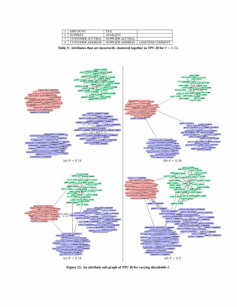
1 DISCOUNT TAX2 SUPPKEY AVAILQTY3 CUSTOMER.ACCTBAL SUPPLIER.ACCTBAL4 CUSTOMER.ADDRESS SUPPLIER.ADDRESS LINEITEM.COMMENT

Table 5: Attributes that are incorrectly clustered together in TPC-H for θ = 0.12.

(a) θ = 0.14 (b) θ = 0.16

(c) θ = 0.18 (d) θ = 0.2

Figure 12: An attribute sub-graph of TPC-H for varying thresholds θ.

appear in the AUTHOR table as well. The same is true for ARTI-CLES.TITLE and INPROCEEDINGS.TITLE, since it seems that themajority of papers submitted to journal publications have the exactsame title as the conference versions of the papers.

Overall, clearly it is in some cases difficult even for humans todecide what constitutes an attribute, without additional applicationdependent context. Our technique is able to separate major at-tributes very well, and make only minor mistakes that can either becorrected by supervision and simple statistical analysis, or by usingorthogonal approaches (e.g., column name matching, if meaningfulschema information exists).

6. RELATED WORKThe work of Zhang et al. [17] was the main impetus behind our

approach, since they introduced the usage of EMD for correlatingcolumns based on the distribution of their values. Zhang et al. in-troduced the quantile approximation of EMD that we also use hereand laid the foundation of using EMD to express primary/foreignkey relationships that are one of our main relationship types. Nev-ertheless, here we extend this work by building distribution andattribute graphs based on EMD and Intersection EMD, which is anovel statistical measure of the relationship between two columns.

In the context of relational databases there has been little workthat concentrates on classifying columns into attributes. The onlyprevious work that we are aware of is by Ahmadi et al. [1], thatutilizes q-gram based signatures to capture column type informa-tion based on formatting characteristics of data values (for exam-ple the presence of ‘@’ in email addresses). The technique buildssignatures based on the most popular q-grams within each col-umn and clusters columns according to basic data types, like emailaddresses, telephone numbers, etc. In that respect, the goal ofthis work is orthogonal to ours: It tries to categorize columns intogeneric data types. Our work takes into account the distribution ofvalues, the distribution with respect to common values, and indi-rect associations through witnesses, as opposed to only using thedistribution of q-grams.

Related work from the field of schema matching has concen-trated on three major themes. The first is semantic schema match-ing that uses information provided only by the schema and not fromparticular data instances. The second is syntactic schema matchingthat uses the actual data instances. The third uses external infor-mation, like thesauri, standard schemas, and past mappings. Mostsolutions use hybrid approaches that cover all three themes. Ourwork falls purely under the second category. Existing data drivenapproaches have not used any distributional information to discoverrelationships between columns, apart from simple statistics. Cur-rent approaches use string-based comparisons (prefix/suffix tests,edit distance, etc.), value ranges, min/max similarity, and mutualinformation based on q-gram distributions [11, 7, 8, 12, 13]. Rahmand Bernstein [15] conducted a survey on schema matching tech-niques.

Previous work tangentially related to discovering attributes isthat on discovering columns that contain similar values. A numberof statistical summaries have been developed for that purpose, in-cluding min-hash signatures [5], and locality sensitive hashing [9].These techniques cannot be used for discovering attributes, sincethey only capture intersection relationships between columns andno distributional information.

7. CONCLUSIONWe argued that discovering attributes in relational databases is an

important step in better understanding and working with the data.Toward this goal, we proposed an efficient solution, based on statis-

tical measures between pairs of columns, to identify such attributesgiven a database instance. Our solution was able to correctly iden-tify attributes in real and synthetic databases with very high ac-curacy. In the future, we plan to investigate whether the tech-niques proposed here can be extended to discover multi-columnattributes (for example when customer names are expressed as sep-arate first/last name columns) and also explore whether informationtheoretic techniques can be used to solve the problem of horizon-tally partitioned attributes (like telephone numbers based on loca-tions).

8. ACKNOWLEDGEMENTThe work of Meihui Zhang and Beng Chin Ooi were in part sup-

ported by Singapore MDA grant R-252-000-376-279.

9. REFERENCES[1] B. Ahmadi, M. Hadjieleftheriou, T. Seidl, D. Srivastava, and

S. Venkatasubramanian. Type-based categorization ofrelational attributes. In EDBT, pages 84–95, 2009.

[2] N. Ailon, M. Charikar, and A. Newman. Aggregatinginconsistent information: Ranking and clustering. Journal ofthe ACM, 55(5), 2008.

[3] N. Bansal, A. Blum, and S. Chawla. Correlation clustering.Machine Learning, 56:89–113, June 2004.

[4] B. H. Bloom. Space/time trade-offs in hash coding withallowable errors. CACM, 13(7):422–426, 1970.

[5] A. Z. Broder, M. Charikar, A. M. Frieze, andM. Mitzenmacher. Min-wise independent permutations.Journal of Computer and System Sciences, 60(3):630–659,2000.

[6] S. Chaudhuri, V. Ganti, and R. Kaushik. A primitive operatorfor similarity joins in data cleaning. In ICDE, page 5, 2006.

[7] R. Dhamankar, Y. Lee, A. Doan, A. Y. Halevy, andP. Domingos. iMAP: Discovering complex mappingsbetween database schemas. In SIGMOD, pages 383–394,2004.

[8] H. H. Do and E. Rahm. COMA - a system for flexiblecombination of schema matching approaches. In VLDB,pages 610–621, 2002.

[9] A. Gionis, P. Indyk, and R. Motwani. Similarity search inhigh dimensions via hashing. In VLDB, pages 518–529,1999.

[10] IBM. CPLEX optimizer. http://www.ibm.com/software/integration/optimization/cplex-optimizer.

[11] J. Kang and J. F. Naughton. On schema matching withopaque column names and data values. In SIGMOD, pages205–216, 2003.

[12] J. Madhavan, P. A. Bernstein, and E. Rahm. Generic schemamatching with cupid. In VLDB, pages 49–58, 2001.

[13] S. Melnik, E. Rahm, and P. A. Bernstein. Rondo: Aprogramming platform for generic model management. InSIGMOD, pages 193–204, 2003.

[14] T. Milo and S. Zohar. Using schema matching to simplifyheterogeneous data translation. In VLDB, pages 122–133,1998.

[15] E. Rahm and P. A. Bernstein. A survey of approaches toautomatic schema matching. The VLDB Journal,10(4):334–350, 2001.

[16] T. P. P. C. (TPC). TPC benchmarks. http://www.tpc.org/.[17] M. Zhang, M. Hadjieleftheriou, B. C. Ooi, C. M. Procopiuc,

and D. Srivastava. On multi-column foreign key discovery.PVLDB, 3(1):805–814, 2010.