Automated selection of an accurate model of avisco-elastic material

A.C . Capelo, L. Ironi, S. TentoniIstituto di Analisi Numerica del C.N.R., Pavia, Italy

liliana@supersl .ian .pv.cnr .it

Abstract

A major problem in the development of a compu-tational environment that can reason about phys-ical systems is its ability to formulate a model.The work here described is part of a research effortaimed at developing a comprehensive environmentthat automates the formulation of the constitutivelaw of an actual visco-elastic material. In outline,we approached the problem in two main stages : atfirst, a library of models of ideal materials is gener-ated, and then an accurate model of an actual ma-terial, which explains the observed response of thematerial to standard experiments, is selected . Themodel library includes both models of ideal ma-terials and their qualitative response to standardexperiments . The models are generated in twodifferent formalisms (Rheological Formulae (RF)and Ordinary Differential Equations (ODE)), byfollowing an enumerative procedure and an ap-proach which is grounded both on a component-connection paradigm and on internal state vari-ables . A class of candidate models, i.e . a class ofODES, for the material is selected from the modelspace through the comparison of the observed be-havior, qualitatively interpreted, with the quali-tative behaviors generated directly from the rhe-ological structures . Then, the most "accurate"model for the real material is chosen within theselected class so that both the goodness of experi-mental data fitting and the number of parametersin the model are "reasonable" . This paper mainlyconcentrates on the methods and algorithms, bothqualitative and quantitative, of model selection.

Keywords: Mathematical modeling, qualitativereasoning, rheology, visco-elastic materials.

IntroductionA crucial issue in automated reasoning about a phys-ical system is the automated formulation of an ap-propriate model of its behavior . Recently, a greatdeal of work in the Qualitative Physics framework

has been addressed to the automated model for-mulation problem, and a number of methods andimplemented systems has been proposed (Addankiet al., 1991 ; Bradley, 1994 ; Crawford et al., 1992 ;Capelo et al., 1993 ; Falkenhaier and Forbus, 1991 ;Ironi and Stefanelli, 1994 ; Iwasaki, 1992 ; Low andIwasaki, 1992 ; Iwasaki and Levy, 1994 ; Nayak, 1994 ;Rickel and Porter, 1994 ; Weld, 1990 ; Weld, 1992) .In these approaches, the model formulation probleminvolves the selection, within a predefined model li-brary, of a model in accordance with a set of assump-tions or a user's query about the system behavior .The model library can contain either complete mod-els of the system under study, each of them character-ized by different assumptions (Addanki et al., 1991),or pieces of knowledge about the physical systems,called model fragments, which are suitably selectedand composed to construct the scenario model (Falken-haier and Forbus, 1991). Whereas in the former casethe formulation of an accurate model can be simplyviewed as a search process through a graph of mod-els, where nodes represent models of the system andarcs represent the assumptions that distinguish twoconnected nodes, in the latter one two different is-sues must be considered: the constructed model hasto be both adequate to describe the physical situationand as simplest as possible (Iwasaki and Levy, 1994 ;Rickel and Porter, 1994).

This paper describes our approach to the automatedmodel formulation of an accurate quantitative model ofthe mechanical behavior of an actual visco-elastic ma-terial (Arridge, 1975) in accordance with the observedbehavior of the material in response to standard ex-periments. The actual difficulties in building by handmodels of materials motivated our work . Knowing theconstitutive laws of materials, i .e . the relation betweenstress s(t) and strain e(t) and their time dependen-cies, allows us both to derive predictions of a mate-rial's behavior under the action of external forces andto associate the material with its mechanical proper-ties . Moreover, the mechanical properties of a materialmay be correlated to some of its other properties (forexample network structure, sensitivity to erosion, hy-

drophilia, capacity either to absorb or to release activeingredients, thyxotropy, and so on), whose knowledgeis of fundamental importance to the assessment of thematerial. The measurement of these latter propertiesoften presents more difficulties than the measurementof the mechanical ones . Hence, the rheological study ofa material may often be both economic and importantin the control of the industrial processing of products .Although our approach has been tailored on a spe-

cific application domain, most ideas and techniquesunderlying it can be applied to other physical do-mains when the goal is to build an accurate quan-titative model explaining a set of experimental data .The whole formulation process occurs in two mainstages : at first, an exhaustive library of complete mod-els of ideal visco-elastic materials, which differ fromeach other in structure, is automatically generated,and then an accurate model of an actual material isbuilt in accordance with the observed response of thematerial to either creep or relaxation experiments.As far as model library is concerned, our work is dis-

tinguished in that it automatically generates the ODEmodels of materials with complex rheological struc-tures. Such structures are automatically enumeratedby analogy with mechanical devices where componentswhich reproduce the fundamental elastic and viscousresponses are combined either in series or in parallel .The symbolic description of such structures is calledRheological Formula (RF). Then, by exploiting suit-able connection rules and mathematical models of thebasic components, which are expressed through inter-nal state variables, the mathematical model ofeach RFis generated. Adequate filter procedures, based on thealgebraic properties of the connection operators andon the mechanical equivalence which is captured bythe ODEs, allow us to control the combinatorial ex-plosion of the model generation process. In a previouspaper (Capelo et al., 1993) we gave a characterizationof the generated ODE models and proved that fourclasses of ODEs represent the space of possible linearmodels of visco-elastic materials. Moreover, it can beproved by induction that the dimension of the modelspace is equal to 2n, where n is the maximum numberof components the RFs are made up . This result is im-portant as understanding the space of possible modelsis an essential step in the construction of computa-tional environments which aim at selecting the mostappropriate model.

This paper focusses on the model selection problemand describes an approach which results to be a mix-ture of qualitative and quantitative techniques withboth symbolic and numeric computations . More pre-cisely, we exploit qualitative reasoning to select theclass of ODEs which describe the qualitative behaviorof the material, and then, within the selected class weidentify the equation, namely the order of the ODEand the numeric values of its parameter, which refinesthe quantitative properties of the material . The se-

lection of the plausible class of models occurs on theground of the qualitative comparison of the simulatedbehaviors of the models in the library with the obser-vations . To this end, algorithms for both qualitativesimulation of the response of materials to creep andrelaxation experiments, and qualitative interpretationof experimental data have been implemented .The selection of the most accurate ODE model is

easily performed when the expert knows the numberof either retardation or relaxation times (Ferry, 1970 ;Whorlow, 1980) as the order of the ODE can be corre-lated with such a number . Therefore, in this case, theselection problem is restricted to a parameter identi-fication problem. When this information is not avail-able, the order of the equation is determined througha technique, borrowed from Statistics, which consistsin minimizing a functional which expresses the balancebetween both the goodness of fitting, which increaseswhen the number of parameters grows, and the signifi-cance of the numerical values of the parameters them-selves, which diminishes when their number grows .

This paper is organized as follows: the next sectiondeals with the approach used for selecting a plausibleclass of models, namely qualitative reasoning meth-ods for simulation and data interpretation . Then, thealgorithm for selecting the most accurate model to-gether with the Akaike (Akaike, 1974) method, whichhas been adapted for solving our optimization problem,are presented .

Selection of the appropriate class ofmodels

Qualitative methods both for simulation and interpre-tation of observations play a key role in the first stageof the model formulation problem. The qualitative in-terpretation of observations gathered from ad hoc de-signed experiments allows us to highlight some proper-ties of the studied material, and consequently to makea guess for a set of its plausible models . The selec-tion of the plausible ODES occurs on the ground of thequalitative comparison of the simulated behaviors withthe observations (Figure 1) .

For the sake of clarity and completeness, we brieflyrecall the basic assumptions, definitions and methodsunderlying our previous work.

Suitable modeling assumptions are made about ma-terials, acting forces and processes . A material is as-sumed to be a continuous, homogeneous and isotropicmedium, and processes take place in isothermal con-dition in order to decouple the thermodynamics as-pects from the mechanical ones . Only stable materi-als are considered and therefore the deformation of abody solely occurs when mechanical energy has beenprovided . As many rheological experiments are car-ried out in one dimension, that is mechanical energy issupplied through longitudinal traction or compressionforces, we only consider one-dimensional deformationprocesses.

Models Library

QUALITATIVEBEHAVIORS

RHEOLOGICALFORMULAE O

ABSTRACTEDQUALITATIVEBEHAVIOR

Quolitctiveinterpretotion

EXPERIMENTALDATA PLOT ~- Rheometer

Figure 1: First stage in model selection: a class ofmodels is selected from the model library in agreementwith the qualitative interpretation of data . Thick linearrows track data flow, while thin ones denote interac-tions within library items

The method adopted for building the model of a ma-terial is based on a component-connection paradigmand on internal state variables. Each fundamental re-sponse, in our case elasticity and viscosity, correspondsto an ideal material which can be represented by a me-chanical analogous device . More precisely, the purelyelastic response is associated with a material H ana-logically represented by a spring whose response is de-scribed by the Hooke's law of linear elasticity s = Ee,where E is a constant which depends on the material .Similarly, the purely viscous response corresponds to amaterial N analogically represented by a dashpot, andis described by the Newton's law of linear viscositys = 77e, where 77, the viscosity coefficient of the mate-rial, is a positive constant and the dot denotes the timederivative . Although the constitutive law of a materialmay be non-linear and may contain non-constant co-efficients, we consider linear visco-elastic models, i.e .models whose visco-elastic behavior is described by anODE with constant coefficients . Nevertheless, mostmaterials show a linear time dependent behavior inthe limit of infinitesimal deformation and even in fi-nite deformation as long as the strain remains below acertain limit, which varies from material to material .

Models of complex materials are built by analogywith mechanical devices, which are obtained by suit-ably assembling, either in parallel or in series, com-ponents which represent the fundamental mechanicalproperties so that the whole device behaves analo-gously to an actual material . The symbolic descrip-tion of an analogical structure, RF, represents a modelof its corresponding material at the lowest level of de-scription.The model library is automatically generated and in-

cludes (1) RFsof all non-equivalent structures made upof n components, (2) the corresponding ODE models,

and (3) the simulated qualitative responses of the gen-erated models to standard experiments. At first, therheological formulae are recursively built and groupedwith respect to equivalence relations: only one repre-sentative for each class is kept in the library. Then, theset of formulae is mapped to its corresponding set ofmathematical models by exploiting the ODE formal-ism, the basic component models and suitable connec-tion rules. More precisely, when components C1 andC2 (not necessarily basic components) are connectedin parallel (ClIC2), they undergo the same elongationwhile the total stress gets distributed among the com-ponents, that is : s = s1 + s2 , e = e1 = e2, whereei, si (i = l, 2) are the internal variables, whose timeevolution is expressed either directly by the basic mod-els or by differential equations obtained by the recur-sive application of the connection rules starting fromthe basic models . If the components are connectedin series (Cl - C2), each component takes the sameload and the total elongation is the sum of the elongation of each component: s = s1 = s2 ,

e = el + e2 .By exploiting the constitutive equations of the basiccomponents and the connection laws, the mathemati-cal model of an arbitrarily complex RF can be recur-sively derived, as described in (Capelo et al ., 1993) .ODE models can be further grouped with respect totheir mechanical behavior by considering the structureof their constitutive equations .

Let us call Formal Equation (FE) the symbolic ODEobtained by giving unitary value to all non-zero coef-ficients of the constitutive equation . In (Capelo et al .,1993) we proved (Theorem 1) that the following fourclasses of equations gather all of the admissible FEs

i-0 i=1where m >_ 0, and D` denotes the i-th time deriva-tive operator. If n is the maximum number of basiccomponents the RFs are made up, it can be provedby induction that the ODE models space is equal to2n . The number of equations in each class (FEi, m) isbetween n/2 and n/2 + 1 .The first stage in the model selection process consists

in taking the class of (FEi,m) which exhibits the samequalitative behavior of the real material out of the set{(FEi , m), i = 1, 2, 3,41 .The qualitative behavior of the material in response

to either a creep or relaxation experiment is character-ized by the presence or absence ofeither strain or stress

m m(FE1, m) 1: D's D` e

i=0 i-0m M+1

(FE2, m) E D's = E D'ei=0 i=1m m+1

(FE3, m) ED= s = 1: D'ei-0 i=0m+1 rn+1

(FE4, m) E D's = 1: D' e

properties, respectively . Therefore, the simulation al-gorithm, as well as the observations interpretation al-gorithm, generates qualitative profiles which highlightsuch physical properties .

Qualitative simulation

The simulation algorithm (Algorithm B), which is anextension and a generalization of the algorithm (Algo-rithmA) previously defined only for creep experiments(Capelo et al., 1993), generates the responses of theideal materials in the library to creep and relaxationexperiments. It operates at the lowest level of descrip-tion, i.e . on the rheological formula, as symbolic in-tegration procedures could be heavy or unfeasible tobe applied, and QSIM-like algorithms (Kuipers, 1986)would fail because of both the need to introduce alargenumber of auxiliary variables in writing the qualitativeversion of the ODES and the consequent difficulty incontrolling the proliferation of the predicted behaviors .

In order to define both the qualitative creep (QB,)and relaxation (QB,) response let us remind that acreep experiment consists of applying an external forceon the material and observing the caused deformation,whereas a relaxation test consists of imposing a de-formation and measuring the corresponding producedstress . According to the input signal shape, we furtherdistinguish in static and dynamic experiments. Statictests involve the instantaneous imposition ofaconstantstress (or strain) and the observation of the subsequentevolution over time of the strain (or stress) . Dynamictests involve the application of an oscillatory input sig-nal. Static experiments highlight the qualitative visco-elastic properties we are interested in better than dy-namic tests, as in the former case the response of thematerial can be analyzed even in the very initial phaseof the experiment, whereas in the latter one it providesuseful information only after a transitory phase. Forthis reason we only consider static tests. The form ofthe applied excitation is suggested by criteria of the-oretical and experimental simplicity . Standard staticexcitations are mathematically modelled by step func-tions of the type :

co[H(t - to) - H(t - ti)]

where to and tl (loading and unloading instants) arethe significant time-points, H(t) is the Heaviside func-tion, and co is constant (Figure 2) .

Creep and relaxation are dual aspects of the samephenomenon: the molecular rearrangements occurringinside a material subjected to external forces dependupon time . When the stress is regarded as the cause,the molecular rearrangements appear at a macroscopiclevel as a retardation of strain : the time required canbe very short if the tested material is elastic, very longif it is viscous, or finite - of the order of the scale ofthe experiment - in the intermediate cases. Similarly,when the stress is regarded as the effect, a stress relax-ation is produced macroscopically over a more or less

CO

load is

load isimposed removed

t o

Figure 2: Standard static test : a stress or a strain issuddenly imposed and then held constant for a timeAt =t1-to

t

Figure 3: A Typical strain response to a stress stepexcitation (creep test)

long time, depending on the mechanical properties ofthe material .The strain response to a step stress excitation re-

sults from the superposition of three basic components,namely an elastic instantaneous eH deformation, a de-layed (still elastic) eK one, and a viscous irrecoverableeN deformation:

a = eH + eK + eN .

Therefore, for example, a purely viscous material,which dissipates all the deformation energy as heatthrough viscous forces, undergoes an irrecoverable de-formation and is characterized by e = eN 54 0, eH =eK = 0. More generally, a visco-elastic material mightstore part of the deformation energy elastically as po-tential energy and dissipate the remaining one vis-cously as heat, featuring a strain response like theone shown in Figure 3, which is characterized byeH, eK, eN 0 0 . Such a material would recover apart of the deformation instantaneously, a part moreslowly, but would also undergo a permanent deforma-tion to a certain extent .The stress response to a step strain excitation results

from the superposition of three stress components :

S =SH+SM+SN ,

each one associated with a mechanical property of thetested material . More precisely: sH $ 0 means thatpart of the undergone stress does not relax at all inthe time interval (to,tl) and denotes the ability ofthe material to store potential energy ; sM :A 0 means

s

to t

Figure 4: A typical stress response to a strain stepexcitation (relaxation test)

that part of the undergone stress relaxes slowly during(to, t1) ; sN 0 0 means that part of the undergone stressrelaxes instantaneously at t = to and the deformationenergy is partially dissipated through viscous forces .As an example, Figure 4 illustrates a stress response

characterized by sH, sM, sN :A 0. Let us remark thatsN 0 0 theoretically corresponds to a Dirac delta func-tion and is graphically represented by a vertical arrowpointing either upward or downward according to thestress impulse sign .

Therefore, both QB, and QB,, can be described byjust three logical parameters (a,,3, 7) which are asso-ciated with either the strain or stress properties, re-spectively, and may take on either the value TRUE(T) or FALSE (F) in accordance with the presence orabsence of the corresponding property in the material .For example QB, = (T, T, T) means that the mate-rial exhibits instantaneous elasticity (eH 54 0), delayedelasticity (eK :0 0) and viscosity (err :A 0) . In order todefine QB, and QB,, for any complex formula, let usremind that, according to the connection rules, strainsare added in series and stresses are added in parallel .Therefore :if QB,:[C1]

QBJC2] = (a2, 02, 72), thenQB,[Ci - C2] = QB,:[C1] V QB~:[C2] _

= (al V a2, )31 V 02, 71 V 72) ;if QB, . [Ci] _ (a1, N1, 71 ), QB,. [C2] = (a2032,72), then

QB,. [Ci I C2] = QB,.[Ci] V QB,. [C2] == (al V a2, 01 V02, 71 V 72),

where V denotes the logical OR operator .It is obvious that QB, and QB,, would be straight-

forward defined for any given complex formula C if itcould be possible to use one of its equivalent formulaewhich is characterized either only by the series oper-ator or only by the parallel one. To this end, in thefollowing we give theorems which state a one-to-onecorrespondence between the classes of ODEs and suit-able classes of rheological formulae (reference classes),and the mechanical equivalence ofany complex formula

with a formula in one of the reference classes . Moreprecisely, let us denote by 0 the mapping of a RF toits respective FE, by K and M the models definedby the formulae HIN and H - N, respectively knownin the literature as Kelvin and Maxwell models, andby Kn,, (M�, respectively) the m-th order generalizedKelvin (Maxwell respectively) models :K�,=K-K- . . .-K

(Mm =MI M~ . . .~M),

and assume, conventionally, that Ko = Mo = 0 . It canbe easily proved by induction on the connection lawsthat for any integer m >_ 0:Theorem 2.

The formulae K� , - H, Kn,, - N,K�,+i, Km-M map to (FE1, m), (FE2 , m), (FE3 , m),(FE4, m), respectively

Q(Km - H) = (FEi, m)Q(K� , - N) = (FE2, m)Q(Km+,) = (FE3, rn)Q(K, - M) = (FE4, m)

Theorem 3.

The formulae Mm JH, M�, I N,Mm I K, M�,+i map to (FE1, m), (FE2, m), (FE3 , m),(FE4, m), respectively

P(M,

H) = (FE1, rn)Q(Mm I N) = (FE2, m)P(M.

K) = (FE3, m)SZ(M�,+i)

= (FE4, m)The formulae mentioned in Theorems 2, 3 are the ref-erence formulae .An important consequence of Theorems 1, 2, 3 is thefollowing duality property :

Theorem 4. Given any arbitrarily complex rheolog-ical formula C, it is possible to find a mechanicallyequivalent formula C_ obtained by combining in seriesa suitable number of components H, N, K, as wellas it is possible to find an equivalent formula C, ob-tained by combining in parallel a suitable number ofcomponents H, N, M.[Proof.If Q(C) = (FEI, m) then set C_ = Km, - H, C1 =Mm I H .If Q(C) = (FE2, m) then set C_ = Km - N, C1 =Mm I N .If Q(C) = (FE3, m) then set C_ = Km+1, C, =Mm I (H I N)-If Q(C) = (FE4 , m) then set C_ = Km - (H - N),C1 = Mm+i - ]

Let us call C_ and C1, chosen as in the above theo-rem proof, equivalent dual (respectively series and par-allel) representations of C. By denoting with Nt theset of all and none but the mechanically distinct RFs,

by Theorem 4 we can state that M is isomorphic tothe dual sets :

M_ = I K,,, - H, K,, - N, K, +,, K�1 - M}

MI = {M. I H, M. I N, M,nI K, Mm+1 }

Therefore, the set of models {H, N, K} plays therole of a "basis" of components for M_ with respectto the series operator, as well as the set {H, N, M}respectively plays a similar role for MI with respect tothe parallel operator .Theorem 4 suggests a natural way of defining both

QB, and QBr associated with any given formula C byconsidering its equivalent representation either C_ inM_ or C in MI, respectively .The algorithm for determining both QB, and QBr

associated with any given formula C is defined as fol-lows:

QBjC] =

~ else, let C be replaced by its seriesequivalent representation C_

QBr [C] =

If C E {H, N, K} then

QB,[H] _ (T, F, F)QBr~ [N] _ (F, F, T)QB,[K] _ (F, T, F)

QBc[Km - H]

QBc[C-] -

QBc[K,n - N]QBc[K�,+1 ]QBc[Km - (H - N)]

If C E {H, N, M} then

QBr [H] = (T, F, F)QBr [N] = (F, F, T)QBr[M] = (F, T, F)

else, let C be replaced by its parallelequivalent representation C

Q&[Mm 1 H]QBr

[CI]=

QBr[M,,, ( N]QBr[Mm I (H I N)]QBr[Mm+1]

The algorithm strictly depends on the applicationdomain . However, its lack of generality is well compen-sated by its completeness and soundness. As a matterof fact ; the given simulation algorithm is the qualita-tive transcription of the connection rules which math-ematically express, through the internal variables, thelinks between either strain or stress and their own re-spective components . With reference to the RFs, thestrain components are added in presence of a series op-erator, whereas the stress ones in presence of a paralleloperator . Therefore, the proof of the soundness of thealgorithm derives straightforward from the connectionrules for the series and parallel operators. The proof

of its completeness is given by Theorems 1-4. Moreprecisely, Theorem 1 defines the elements (FE) of theset of the admissible ODE models ; Theorems 2 and 3respectively state a bijective correspondence betweenFEs and RFs (elements of both sets M_ and MI),which are built by connecting either in series the ele-ments of the set {H, N, K} or in parallel the elementsof the set {H, N, M} . Finally, Theorem 4 associatesany complex given formula, by exploiting its FE, withits equivalent representation both in M_ and in MI .Although in terms of computational efficiency Algo-

rithms A and B are comparable, version B marks asignificant improvement . In fact, Algorithm B is fullyjustified from the formal point of view as it is basedon sound arguments such as the connection rules andFEs, whereas Algorithm A, which recursively buildsthe response of the material starting from the qualita-tive behavior of the elements H and N, is partly sug-gested by the connection rules and partly by intuitivephysical arguments. Moreover, Algorithm B works forboth creep and relaxation tests.

Finally, let us observe that, although Algorithm Bhas been given, for the sake of simplicity, for inputsignals represented by step functions, it also holds forinput signals represented by a summation of step func-tions. This is ensured by the linearity of the ODEs or,equivalently, by the Boltzmann principle of superposi-tion .

Qualitative interpretation of experimentaldata

Qualitative interpretation of experimental data, i.e .their characterization in terms of relevant qualitativephysical features, is an important step in view ofmodel selection (Forbus, 1987 ; DeCoste, 1991 ; McIl-raith, 1989) .

Quite generally, physical features can be capturedthrough the identification of characteristic shapes inthe experimental data plot . Therefore, in order to rea-son qualitatively about the observed response, graphi-cal data are first abstracted to a qualitative represen-tation : a qualitative curve description is automaticallyprovided in terms of regions which are homogeneouswith respect to such graphical features as steepness,convexity and linearity. This process of data segmen-tation takes its basic ideas from pattern recognitionand qualitative physics . We would like to remark that,though here applied to a specific domain, the adoptedapproach is quite general.In the following, for the sake of simplicity and to bet-ter focus on methodologies, we limit our attention tocreep experimental data . As a matter of fact, analysisof relaxation data can be carried out in quite a sim-ilar way by suitably extending the numeric descrip-tors and thresholds spaces as well as the vocabularyof qualitative curve attributes, in order to account forrelaxation-specific graphical features .Suitable numeric curve descriptors, namely the strain,

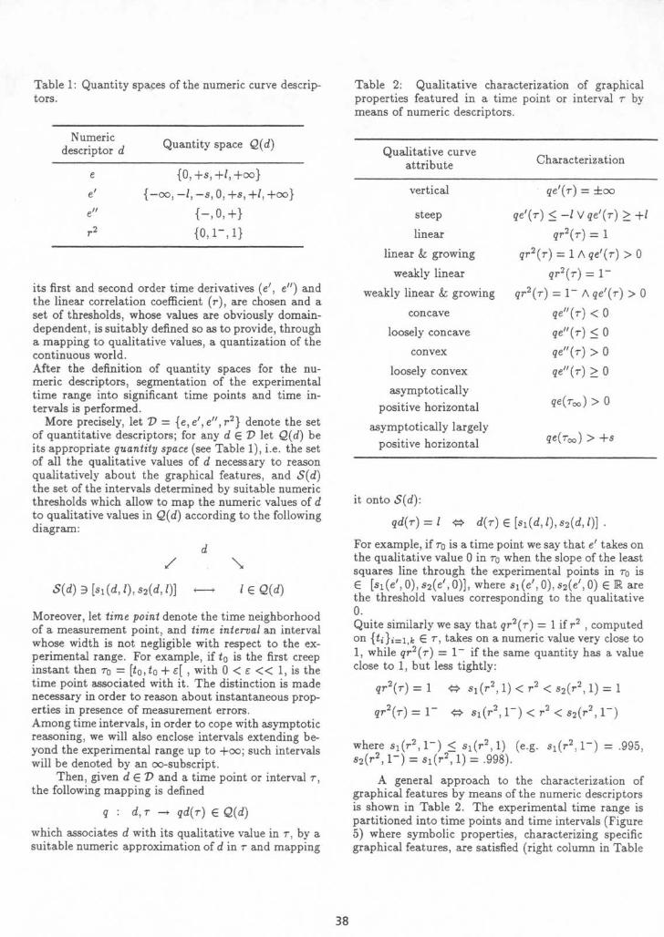
its first and second order time derivatives (e', e") andthe linear correlation coefficient (r), are chosen and aset of thresholds, whose values are obviously domain-dependent, is suitably defined so as to provide, througha mapping to qualitative values, a quantization of thecontinuous world.After the definition of quantity spaces for the nu-meric descriptors, segmentation of the experimentaltime range into significant time points and time in-tervals is performed .More precisely, let D = {e, e', e", r2} denote the set

of quantitative descriptors; for any d E D let Q(d) beits appropriate quantity space (see Table 1), i.e . the setof all the qualitative values of d necessary to reasonqualitatively about the graphical features, and S(d)the set of the intervals determined by suitable numericthresholds which allow to map the numeric values of dto qualitative values in Q(d) according to the followingdiagram:

S(d) E) [si (d,1), s2 (d,1)]

-

1 E Q(d)

Moreover, let time point denote the time neighborhoodof a measurement point, and time interval an intervalwhose width is not negligible with respect to the ex-perimental range. For example, if to is the first creepinstant then ro = [to, to + E[ , with 0 < E << 1, is thetime point associated with it . The distinction is madenecessary in order to reason about instantaneous prop-erties in presence of measurement errors .Amongtime intervals, in order to cope with asymptoticreasoning, we will also enclose intervals extending be-yond the experimental range up to +oo ; such intervalswill be denoted by an oo-subscript .

Then, given d E D and a time point or interval r,the following mapping is defined

q :

d, r -} qd(r) E Q(d)

which associates d with its qualitative value in r, by asuitable numeric approximation of d in 7 and mapping

linear & growing

weakly linear

weakly linear & growing

concave

loosely concave

convex

loosely convex

asymptoticallypositive horizontal

asymptotically largelypositive horizontal

it onto S(d) :

gr2 (r) = 1A qe'(r) > 0

gr2 (r) = 1-

gr2 (r) = 1 - A qe'(r) > 0

qe"(r) < 0qe"(r) < 0qe"(T) > 0qe"(r) > 0

qe(r,,) > 0

qe(r,,.) > +s

qd(T) = 1

q

d(T) E [si(d,1), s2 (d,1)] .

For example, if ro is atime point we say that e' takes onthe qualitative value 0 in To when the slope of the leastsquares line through the experimental points in ro isE [s, (e', 0), s2(e', 0)], where si(e', 0), s2(e', 0) E 118 arethe threshold values corresponding to the qualitative0.Quite similarly we say that gr2(,r) = 1 if r2 , computedon {ti}i=i,k E r, takes on a numeric value very close to1, while gr2 (r) = 1 - if the same quantity has a valueclose to 1, but less tightly :

gr2(r) = 1

<* si (r2,1) < r2 < s2 (r 2 ,1) = 1

gr2(T) = 1 -

q si(r 2 ,1 - ) < r2 < s2(r2

, 1 -)

where s, (r2 ' 1- ) <_ si(r2 , 1)

(e.g.

si (r2 , 1- ) = .995,$2(r

2, 1- ) = si(r2

, i) = .998) .

A general approach to the characterization ofgraphical features by means of the numeric descriptorsis shown in Table 2 . The experimental time range ispartitioned into time points and time intervals (Figure5) where symbolic properties, characterizing specificgraphical features, are satisfied (right column in Table

Table 1 : Quantitytors .

spaces of the numeric curve descrip- Table 2 : Qualitativeproperties featured in

characterization of graphicala time point or interval r by

means of numeric descriptors .

Numericdescriptor d

Quantity space Q(d)Qualitative curve

attribute Characterizatione {0, +s, +1, +oo}

e' {-oo, -1, -s, 0, +s, +1, +oo} vertical qe'( ,r) = foo

e// {-, 0, +} steep qe'(r) < -1 Vqe'(r) > +1

r2 {0,1 - ,1} linear gr2(T) = 1

TO Tde0e

TvT1Tde

Tmt

Figure 5: Data segmentation in view of qualitativecurve description

2) ; the experimental data plot is then described by thesequence of the qualitative curve attributes (from thevocabulary in the left column) which are appropriatefor each time segment .Assessment of the observed qualitative behaviorIn the case of creep data, two experimental stages canbe distinguished : creep, which is related to loading im-position and holding time [to, tl [, and recovery, relatedto loading removal [t1, +oo[ . As a matter of fact, ei-ther stage can provide enough information to assess in-stantaneous elasticity, delayed elasticity and viscosity.However, since data are always affected by measure-ment errors, reasoning about data can take advantageof both creep and recovery curve analysis . For the samereason, in the definition of clauses we require that eachproperty is weakly satisfied in both creep and recoveryand strongly in at least one of them .In the light of the above considerations, the key clausesfor the assessment of each mechanical feature are nowdescribed .Instantaneous elasticity:This property consists in the material ability at yield-ing a prompt deformation to loading and unloading(see Figure 3) . Strain jumps at to and tl graphi-cally characterize instantaneous elasticity . Due to theinstrument limitations at coping with instantaneousevents, namely the instrumental inertia combined withthe measurement errors, this property is captured byreasoning about the curve steepness on time-points To,71 :

if curve isvertical at To AND steep at 71OR steep at To AND vertical at 71

thenproperty-1 is instantaneous-elasticity

elseproperty-1 is NOT-instantaneous-elasticity

endif

(Of course, in accordance with Table 2, verticalat To AND vertical at 71 implies property-1 isinstantaneous-elasticity .)

Viscosity:

The presence of a constant positive deformation rate inthe late creep stage is due to energy dissipation . Cor-respondingly on recovery the material is not able to getback to the original length . Therefore, an eventuallylinear growth at late loading or, equivalently, a finitepositive residual as t goes to infinity characterize thisproperty .As regards the creep stage, the significant time intervalcan be identified as follows:

where mint {t I gr2 (t, tl ) = 1 denotes the first instantof the linear region . Similarly a time interval T,-, isdefined to characterize a weakly linear region . On re-covery, in order to reason about asymptotic attributes,a time interval Too := [T, +oo[ , T >> ti is implic-itly introduced . The qualitative value of the asymp-totic strain ge(Too) is derived by an approximation oflimt-oo e(t) obtained by extrapolating the late recov-ery points under a simple exponential decay model .

By combining creep and recovery reasoning, vis-cosity is finally assessed as follows :if curve islinear-and-growing at T�ANDasymptotically-positive-horizontalOR weakly-linear-and-growing at 7v-

ANDasymptotically-largely-positive-horizontal

thenproperty-3 is viscosity

elseproperty-3 is NOT-viscosity

endif

Delayed elasticity :

Tv :- [min{t I gr2(t,il) = 1} , tlt

1,

In order to reason about delayed elasticity the curveconcavity must be ascertained, even when data are af-fected by measurement errors . The expert would per-form a subjective visual smoothing which can be emu-lated in a number of ways . A simple and quite naturalapproach consists in reasoning by intervals rather thanpoint-wise ; first the time interval to analyze Tde (Tae forcreep and Tae for recovery, respectively) is divided intosubintervals Tde = UhTh, and then for each subintervalqe"(Th) is taken as the most frequent of the pointwisecomputed signs of e" . Therefore:Tde := [to, tl[ \(To U 7J)

if Taethenproperty-2 is NOT-delayed-elasticity

elseperform interval partitioning Tae = UhThif curve isloosely-concave at any Th

An example

Bir j

Data plot )' ~-abstraction )

Plausible models

;Done

MATERIAL : INK 3322/06 1

QUALITATIVE CURVE DESCRIPTION

Ct-0) concave(t-de-0) linear&groaing(t v)

steep(t1) convex(tde-1) largely-positive(t_in'ty)

CREEP :

RECOVERY :

ASSESSED QUALITATIVE BEHAVIOR : CF,T,T)

FEATURED PHYSICAL PROPERTIES :

Figure 6: Selection of the plausible models class for an ink-like material

ANDconcave for at least one

thenproperty-2 is delayed-elasticity

elseproperty-2 is NOT-delayed-elasticity

endifendif

Th

The above clause is actually made more robust by in-cluding reasoning about the convexity of the recoverycurve.

As an example, let us consider the observed data froma creep experiment performed on an ink-like material .Figure 6 is a screen dump which displays a plot ofthe observations, and the featured physical propertiesattributed to the shape of the plot (delayed elasticityandviscosity) . As a result of the match of the identifiedstrain characteristics (eH =F, eK =T, eN =T) againstthe qualitative simulated behaviors of ideal materials, aclass ofplausible candidate mathematical models of thematerial is automatically provided . For the materialin the example, 9 candidate models, whose equationsare of the form E'o D=s D= e (where m =1, . . ., 9) are generated.

Selection of the accurate model

Given the class (FE=, m) of ODE models which exhibitthe same qualitative behavior as the actual material,the selection problem consists in identifying an equa-tion Et which refines the quantitative properties of thematerial . E= is the equation of order k whose para-metric coefficients have been assigned numeric valuesso that it better fits the experimental data . There-fore, in order to solve the problem we have to deter-mine both the order k of the equation and the nu-meric values of its parametric coefficients, whose num-ber n obviously depends on k (n(k)) . It is clear thatif the order of the equation is increased, and conse-quently the number of the parameters is increased, thegoodness of fitting improves, but the significance ofthe numerical values of the parameters themselves di-minishes . On the other hand, also the possibility togive a physical interpretation of these numerical val-ues can fail, and even more important, the informationabout the number of retardation times (Ferry, 1970 ;Whorlow, 1980), which is a feature of the material andis strictly related to the order of the model equation,can be lost if we restrict the problem to the goodnessof fitting .

Let us remind that the retardation times are pa-rameters associated with the material state changeswhich subsequently occur. For example, in polymeric

materials they can be associated with the break of ei-ther the hydrogen or Van der Waals bounds which doesnot occur at simultaneous times . From the modelingpoint of view, the retardation times are specified inthe arguments of exponential functions whose sum de-fines the solution of the ODE model. In some cases,the expert can estimate the number of state changesthe material will undergo during the rheological tests,and then the number of retardation times. When theuser has such a knowledge, the selection problem isrestricted to a parameter identification one (Figure 7(a)) . By exploiting arguments based on the Laplacetransform, it can be proved that there is a correlationbetween the number of retardation times and the or-der of the equation which describes the behavior of thematerial . Therefore, the order k, and consequently thenumber of parameters is straightforward fixed. Moreprecisely, if k is the number of retardation times, theorder of the most plausible ODE model is equal to k ifthe selected class is either FE, or FE3, and equal tok + 1 in the other two cases . Then, the most accuratemodel of the material can be determined by comput-ing, through ad hoc implemented techniques of fittingof experimental data, the values of the parametric co-efficients which appear in (Ei, k) .

The problem is more complex if no information isprovided about the ODE order. In such a case, thequantitative model is obtained through an optimization technique whose goal is to determine the optimalorder k of the equation Ei so that both the goodnessof fitting and the significance of the identified numeri-cal values of parameters are guaranteed . The selectedclass of plausible ODES is made up of equations E;which differ in the order but not in the structure, i.e .(Ei, k + 1) differs from (Ei, k) only for the presenceof terms which express the (k + 1)-derivative of eitherstress or strain . An analogous situation can be foundin the theory of time series where the problem to de-termine the order of the model (e .g . AutoRegressiveMoving Average (ARMA) model) is quite important(Choi, 1992). In this context several methods havebeen proposed, and among those we consider the AIC(Akaike Information Criterion) method (Akaike, 1974).In our case, such a criterion can be formulated as fol-lows :

(Akaike Criterion) The equation of order k whichbest fits the experimental data corresponds to theequation whose number of parameters n(k) is the min-imum of the function :

(1) AIC(n(k)) = 2n(k) - 21og[maximized likelihood] .

It can be proved that the order k estimated in sucha way is never lower than the actual order of the Eiwhich describes the behavior of the material . It canbe straightforward proved that if, as it is plausible inour case, the experimental errors are independent andnormally distributed, the maximum likelihood method

QUANTITATIVEMODEL

Figure 7: Second stage in model selection: (a) if thenumber of retardation times is supplied by the User,a single ODE is selected and the quantitative model isobtained by parameter identification ; (b) if no informa-tion is provided about the ODE order, the quantitativemodel is obtained through an optimization technique

corresponds to the least squares method . Therefore,apart from constant additive terms, the function (1)becomes:

(2)

AIC(n(k)) = 2n(k) + m logS2(n(k)),

where m is the number of experimental data andS2(n(k)) the sum of the squares of residuals when thefitting is performed with a model with n(k) parame-ters .

From the algorithmic point of view, the value ofn(k) which minimizes the function (2) is calculatedthrough a loop (Figure 7 (b)) whose main steps are:

" selection of an equation (Ei, k)," parameter identification of the n(k) parameters in

(Ei, k),

" evaluation of AIC(n(k)),

" comparison of AIC(n(k - 1)) with AIC(n(k)) andloop termination if AIC(n(k - 1)) < AIC(n(k)),since in general the function (2) is convex .

The output of the loop, i .e . the quantitative ODEmodel of order k - 1 with n(k - 1) coefficients is anaccurate model of the behavior of the material as itguarantees both the goodness of data fitting and thesignificance of the numerical values of its coefficients .

DiscussionWe presented an approach to the automated formula-tion of an accurate quantitative model of the behaviorof a visco-elastic material. Such a model can be ex-ploited by the expert for a precise analysis of the ma-terial during its assessment phase. More precisely, itcan be numerically simulated to predict the behavior ofthe material under any complex load, and the param-eters in the model could be interpreted as a measureof some properties of the material itself. As far as thelatter use of the model is concerned, there is a need fora rationale which allows us to correlate the parametersin the model and physical properties of materials. Thisissue could be a new challenge in the study of materi-als, which has been performed at a pure experimentallevel so far.

The model selection process occurs in two mainstages : the first stage is performed at a pure quali-tatively level and produces the class of models whichqualitatively describe the material behavior, the sec-ond one, which occurs at a pure quantitative level byexploiting both statistical and numerical methods, gen-erates the quantitative model of the material . Themodel is selected within a library of models which areautomatically generated by connecting variously eitherin series or in parallel 20 basic components . The re-striction of the number of components to 20 is rea-sonable as structures made up of 20 elements are as-sociated with rather complex materials. As the modelspace dimension is equal to 40, it could seem reasonable

to select directly the accurate quantitative model byextending the optimization loop in Figure 7 (b) to thewhole set of models in the library instead of selectingfirst a class of plausible models . There are at least tworeasons why both two steps are necessary. The mostimportant reason is that there is no guarantee thatthe "best" model obtained through the data fitting bymeans of all the models results to be compatible, inqualitative terms, with the observations, or, in otherwords, that it does capture some important features ofthe material (e.g . instantaneous elasticity) . Moreover,the computational cost of parameters identificationgrows significantly with the number of models . Sucha number is actually not too large as we only considerlinear models of visco-elastic materials but it could bequite high as soon as the library is extended both withnon-linear models, which will be built starting fromnon-linear laws, e .g . s(t) = kl(exp(k2e(t)) - 1), ands(t) = kl log(k2 e'(t)), for the elastic and viscous basiccomponents respectively, and with models which takealso plasticity into account. Therefore, the qualitativestage seems to be essential for both an efficient andphysically correct approach to model selection.

The paper gives some contribution to qualitativereasoning methods: both qualitative simulation anddata interpretation methods ad hoc implemented forour specific goal have been presented. The simulationalgorithm is strictly domain-dependent but generatesall and none but the actual physical behaviors. Thedata interpretation algorithm provides reasoning tech-niques to emulate the expertlike visual interpretationof experimental data . It has been tested on experimen-tal data related to different polymeric materials, suchas inks, rubbers, and drugs (sodium carboximethyl-cellulose) and its performance has been evaluated inaccordance with the interpretation provided by the ex-perts who supplied the data . In spite of its simplicity,the algorithm provides also useful information aboutthe adequacy of the models in the library to describethe behavior of the material under study : a possibleconvex shape of the data during the creep phase de-notes that the linear theory of elasticity and viscositywe adopted to build the model library is inadequate tostudy such a material . Although it has been designedfor interpreting data in a specific domain, it results tobe a domain-independent technique as it is capable totrasform a stream of observed data into a qualitativedescription that characterizes its shape, that is it high-lights the qualitative properties of the numerical datasuch as monotonicity, convexity and linearity regions.

AcknowledgementWe would especially like to thank C. Caramella of theDepartment of Pharmaceutical Chemistry of the Uni-versity of Pavia and B. Pirotti of the PABISCH S .p.A- Scientific Division who provided us with the experi-mental data .

ReferencesAddanki, S.R . ; Cremonini, R. ; and Penberthy, J .S .1991 . Graphs of models . Artificial Intelligence51 :145-177 .

Akaike, H . 1974 . A new look at the statisticalmodel identification . IEEE Trans . Automatic Con-trol 19:716-723.

Arridge, R.G .C. 1975 .

Mechanics of Polymers.Clarendon Press, Oxford .

Bradley, E. 1994 . Automatic construction of accuratemodels of physical systems. In Proc . 8th InternationalWorkshop on Qualitative Reasoning, Nara . 13-23 .

Capelo, A.C . ; Ironi, L . : and Tentoni, S . 1993 . Amodel-based system for the classification and anal-ysis of materials. Intelligent Systems Engineering2(3) :145-158 .

Choi, B. 1992 . ARMA Model Identification . Springer,New York .

Crawford, J . ; Farquhar, A . ; and Kuipers, B.J . 1992 .QPC : A compiler from physical models into qualita-tive differential equations . In B. Faltings, P. Struss,editor 1992, Recent Advances in Qualitative Physics .MIT Press. 17-32 .

DeCoste, D . 1991 . Dynamic across-time measurementinterpretation . Artificial Intelligence 51:273-342 .Falkenhaier, B. and Forbus, K.D . 1991 . Composi-tional modeling : finding the right model for the job.Artificial Intelligence 51 :95-143.

Ferry, J .D . 1970 . Viscoelastic Properties of Polymers.John Wiley, New York.

Forbus, K.D. 1987 . Interpreting observations of phys-ical systems. IEEE Transactions on Systems, Man,and Cybernetics 17:350-359 .Ironi, L . and Stefanelli, M. 1994 . A framework forbuilding and simulating qualitative models of com-partmental systems. Computational Methods andPrograms in Biomedicine 42 :233-254 .

Iwasaki, Y . and Levy, A.Y . 1994 . Automated modelselection for simulation . In Proc . AAAI-9/,, Los Altos.Morgan Kaufmann .Iwasaki, Y. 1992 . Reasoning with multiple abstrac-tion models . In Faltings, B. and Struss, P., editors1992, Recent Advances in Qualitative Physics . MITPress . 67-82.Kuipers, B.J . 1986 . Qualitative simulation . ArtificialIntelligence 29:280-338 .Low, C.M. and Iwasaki, Y. 1992 . Device modellingenvironment : an interactive environment for mod-elling device behaviour. Intelligent Systems Engineer-ing 1(2) :115-145 .Mcllraith, S.A. 1989 . Qualitative data modeling : ap-plication of a mechanism for interpreting graphicaldata . Computational Intelligence 5:111-120.

Nayak, P.P . 1994 . Causal approximations . ArtificialIntelligence 70 :277-334 .Rickel, J . and Porter, B . 1994 . Automated modelingfor answering prediction questions: Selecting the timescale and system boundary . In Proc . AAAI-91,, LosAltos . Morgan Kaufmann .Weld, D.S . 1990 . Approximation reformulations . InProc. AAAI-90, Los Altos . Morgan Kaufmann . 407-412.Weld, D.S . 1992 . Reasoning about model accuracy.Artificial Intelligence 56 :255-300 .Whorlow, R. 1980 . Rheological Techniques . Ellis Hor-wood, Chichester .