AUTOMATED SYSTEM FOR LOAD-BALANCING EBGP...

AUTOMATED SYSTEM FOR LOAD-BALANCING EBGP PEERS

By

BRIAN T. WALLACE

A THESIS PRESENTED TO THE GRADUATE SCHOOL OF THE UNIVERSITY OF FLORIDA IN PARTIAL FULFILLMENT

OF THE REQUIREMENTS FOR THE DEGREE OF MASTER OF ENGINEERING

UNIVERSITY OF FLORIDA

2004

Copyright 2004

by

Brian T. Wallace

This document is dedicated to my wife, Robin, and our children, Parker, Taylor, and Peyton.

ACKNOWLEDGMENTS

I would like to acknowledge the contribution that Dr. Joe Wilson has made to my

academic career. Dr. Wilson has provided me with guidance and inspiration throughout

my course of study. He has worked with me to ensure my success both while in-

residence and as a FEEDS student.

I thank my family for their support during my time as a graduate student. Robin,

Parker, Taylor, and Peyton have been understanding of the requirements of completing an

advanced degree and have provided me motivation to be successful.

iv

TABLE OF CONTENTS page ACKNOWLEDGMENTS ................................................................................................. iv

LIST OF TABLES............................................................................................................ vii

LIST OF FIGURES ......................................................................................................... viii

ABSTRACT.........................................................................................................................9

CHAPTER

1 INTRODUCTION ........................................................................................................1

Internet Routing Protocols............................................................................................1 Classful Network Addressing................................................................................2 Classless Internet Domain Routing (CIDR) ..........................................................2

Interior and Exterior Routing Protocols .......................................................................3 Distance Vector Algorithms ..................................................................................3 Link-State Routing Algorithms .............................................................................4

BGP Overview..............................................................................................................4 BGP Attributes ......................................................................................................5 BGP Best Path Algorithm .....................................................................................5 AS Path Pre-pending .............................................................................................6 Adjusting Multi-Exit Discriminator (MED) Values..............................................8

Network Traffic Collection...........................................................................................8 Simple Network Monitoring Protocol (SNMP) ....................................................9 Promiscuous Mode Packet Capture.......................................................................9 Network Flow Collection ....................................................................................10

2 NETWORK DATA COLLECTION ..........................................................................12

Topology Collection ...................................................................................................12 Fully Automated Solution ...................................................................................12 Database Approach..............................................................................................13

Topology Module .......................................................................................................13 Prefix Tree Generation ........................................................................................14 Circuit Representation .........................................................................................15

NetFlow Data Collection ............................................................................................15 Definition of a Flow ............................................................................................15

v

Capturing NetFlow Data......................................................................................16 Exporting NetFlow data ......................................................................................18 Storage of NetFlow Cache Entries ......................................................................18 Data Collector......................................................................................................19

Traffic Assignment .....................................................................................................21 3 DATA ANALYSIS ....................................................................................................23

Network Data Analysis...............................................................................................23 Analysis Methodology Overview........................................................................24

First pass analysis.........................................................................................25 Second pass analysis ....................................................................................26

Balanced Traffic Condition .................................................................................27 Configuration Generator.............................................................................................29

Benefits of Code Generation ...............................................................................29 Implementation Process.......................................................................................30

4 SYSTEM RESULTS ..................................................................................................34

Testbed Configuration ................................................................................................34 Traffic Generation ......................................................................................................35 Test Cases ...................................................................................................................37 System Output ............................................................................................................38

Test Case #1 ........................................................................................................38 Test Case #2 ........................................................................................................39 Test Case #3 ........................................................................................................40 Test Case #4 ........................................................................................................41

Conclusions.................................................................................................................41 5 SUMMARY AND FUTURE WORK ........................................................................43

System Improvement ..................................................................................................43 Instantaneous Data Rate Load-Balancing ...........................................................43 Low Utilization Prefixes......................................................................................45 Minimizing Prefix Announcements ....................................................................46

Cost Factor in Load Balancing ...................................................................................46 Support More Complicated Route-Maps....................................................................47 Fault Detection............................................................................................................48 Infected Host Detection ..............................................................................................48 Summary.....................................................................................................................48

LIST OF REFERENCES...................................................................................................50

BIOGRAPHICAL SKETCH .............................................................................................51

vi

LIST OF TABLES

Table page 1-1 Bit patterns associated with the original address classes for IPv4. ............................2

2-1 Fields in a NetFlow header packet. ..........................................................................20

2-2 Fields in a NetFlow flow record...............................................................................21

4-1 Subnets that were utilized during lab testing............................................................36

4-2 Description of test cases used during validation testing. .........................................37

4-3 Per circuit loading results from test case #1.............................................................38

4-4 Per prefix loading results from test case #1. ............................................................38







vii

LIST OF FIGURES

Figure page 1-1 The AS path attribute can be modified to implement BGP routing policy. ...............7

1-2 The multi-exit discriminator (MED) attribute can be modified to implement BGP routing policy. ............................................................................................................8

2-1 Tree structure generated by Prefix.pm. ....................................................................14

2-2 Enabling NetFlow on a router interface. ..................................................................16

2-3 Output from router verifying NetFlow configuration. .............................................17

2-4 Configuring NetFlow export on a router interface...................................................18

2-5 Process for transferring data from NetFlow cache to data collection system. .........19

2-6 Process of assigning traffic to a prefix object. .........................................................22

3-1 Process by which router applies BGP routing policy via route-maps and prefix-lists.31

3-3 IP prefix list configuration to identify groups of prefix that will have routing policy applied. .....................................................................................................................32

3-4 Route-maps use prefix-lists to apply routing policy to outbound BGP announcements. ........................................................................................................33

4-1 A typical access network configuration. ..................................................................35

4-2 Lab setup used to test BGP load-balancing tool. .....................................................36

5-1 Total volume of traffic is predictable on a day-to-day basis and grows linearly over time...........................................................................................................................44

5-2 System generated prefix lists are balanced based on load, but not necessarily balanced on number of addresses.............................................................................46

viii

Abstract of Thesis Presented to the Graduate School of the University of Florida in Partial Fulfillment of the Requirements for the Degree of Master of Engineering

AUTOMATED SYSTEM FOR LOAD-BALANCING EBGP PEERS

By

Brian T. Wallace

December 2004

Chair: Joseph N. Wilson Major Department: Computer and Information Science and Engineering

The goal of this project was to develop a system that could analyze network traffic

and topology in order to generate load-balanced router configurations. The motivation

for this effort is that the existing process today is manual, intensive, and potentially error

prone.

The system collects and stores NetFlow data from BGP routers. Traffic data are

assigned to IP prefixes that are valid with an AS. These prefixes are then assigned across

the set of egress links for the AS. A best fit decreasing (BFD) approach is used to

generate a load-balanced condition. If the load is not balanced, IP prefixes are split along

CIDR boundaries and another iteration of the BFD approach is performed.

Test results demonstrate that the system for generating load-balanced BGP

configurations works correctly. Regardless of the complications added to each test case,

the system was able to achieve the desired result.

This study has shown that load-balanced BGP configurations can be developed in

an automated fashion by analyzing traffic data and network topology.

ix

CHAPTER 1 INTRODUCTION

As the Internet has experienced explosive growth in recent years, service providers

have struggled to build capacity and stay ahead of increasing bandwidth demands.

Routing on the Internet backbone is key to maintaining robust global network

communications infrastructure.

This thesis presents an automated method for generating load-balanced Border

Gateway Protocol (BGP) configurations. While traffic patterns on the Internet are

constantly changing, router configuration among External Border Gateway Protocol

(EBGP) peers is basically static. This study will demonstrate an automated tool for

analyzing traffic patterns and developing router configuration to provide a load-balanced

state. This system will be an improvement of the present manual process of determining

configuration changes for BGP peers.

Internet Routing Protocols

The Internet has no shortage of protocols. Of interest in this context is the routing

protocols that are supported and play a role in provide global connectivity via the

Internet. An important distinction must be drawn between routed and routing protocols.

Routed protocols are the protocols used to exchange information between hosts. Routing

protocols are used to convey information among routers and make decisions on path

selection across a network (Stallings 2000).

1

2

Classful Network Addressing

The original Internet routing scheme included addresses classes. Most

organizations were assigned Class A, B, or C networks (Tannenbaum 1996). Class D

address space is reserved for multicast applications. Since multicast addresses are shared

by a group of hosts, the number of hosts per network is not applicable. Class E address

space is reserved as experimental but has never been used in any significant way. In

classful network addressing, the class of an address can be determined by the first four

bits of the address. Table 1-1 illustrates the bit patterns associated with each class. An x

indicates that the bit in that location is not relevant.

Table 1-1 shows the bit patterns associated with the original address classes for IPv4.

Address Class Bit pattern # of networks # of hosts / network

Class A 0xxx 128 16,777,214

Class B 10xx 16,384 65,534

Class C 110x 2,097,152 253

Class D 1110 268,435,456 n/a

Class E 1111 n/a n/a

Classless Internet Domain Routing (CIDR)

These class boundaries developed originally did not survive the rapid expansion of

the Internet and a new technique was required. Network address classes did not scale

with the size of the Internet because this method of allocation could not match the size of

networks being attached to the Internet. For most organizations, a Class A network was

far too large but a Class C networks was too small. This led to many Class A networks

going unallocated while Class B networks were being rapidly depleted. In addition,

3

small companies were allocated a Class C network and wasted the portion they did not

require.

Classless Internet Domain Routing (CIDR) was developed to overcome the rapid

exhaustion of IPv4 address space. RFCs 1518 and 1519 describe a technique where the

subnet mask is a critical piece of information included in routing updates and stored in

routing tables. CIDR lifts the restriction that networks have to be divided on classful

boundaries.

Interior and Exterior Routing Protocols

Routing protocols can be broken into two categories: interior and exterior. Interior

gateway routing protocols (IGPs) are used for internal routing. Typically, all routers

participating in an IGP are under a single administrative authority.

There is a variety of interior gateway routing protocols deployed today. Some

examples of IGPs include Open Shortest Path First (OSPF), Enhanced Interior Gateway

Routing Protocol (EIGRP), Intermediate System – Intermediate System (IS-IS), and

Routing Information Protocol (RIP). While there are a number of IGPs deployed, the

dominant exterior gateway routing protocol is the Border Gateway Protocol.

IGPs are classified based on how they calculate routing metrics. The two primary

classifications are: distance vector and link-state algorithms.

Distance Vector Algorithms

Distance vector algorithms use a simple metric that takes into account spatial

locality. The metric most often used is hop count. Hop count is the number of routers

that must be transited to arrive at the destination. It is possible for a path that is longer

via hop count to yield network performance that is actually better due to additional

bandwidth and lower latency interfaces.

4

RIP is the most common distance vector algorithm deployed. It is easy to

configure and easy to use but does not take into account network performance or

degradation when assigning metrics.

Link-State Routing Algorithms

Link-state algorithms maintain a database of link state information. Whenever a

router participating in a link-state algorithm experiences a change in one of it’s directly

connected interfaces, a link state advertisement (LSA) is sent to all neighboring routers

participating in the same routing protocol. These updates are propagated through the

networks so that all routers have the same topology and state information.

Maintaining a database has both advantages and disadvantages. One significant

advantage is extremely fast convergence. The disadvantage is that the router must

maintain this database entirely separately from the routing table. This increases both the

CPU and memory requirements of a router running a link state routing protocol.

The OSPF routing protocol is by far the most common link state routing protocol.

It is standards-based and performs extremely well.

While maintaining a link state database provides the information necessary for fast

convergence times and consistent routing information, it also does not scale to the level

of the Internet. The amount of traffic generated just by routing updates would flood the

backbone.

BGP Overview

Four regional Internet registries provide the allocation and registration service for

the Internet. The resources assigned by these entities include IP addresses and

Autonomous System numbers. Autonomous systems (ASs) in North America, a portion

of the Caribbean, and sub-equatorial Africa are assigned by the American Registry for

5

Internet Numbers (ARIN). For Europe, the Middle East, northern Africa, and parts of

Asia, allocation and registration services are provided by RIPE Network Coordination

Center (RIPE NCC). The Asia Pacific Network Information Centre (APNIC) is

responsible for the majority of Asian countries. Lastly, The Latin American and

Caribbean IP address Regional Registry is responsible for South America and the

Caribbean islands not covered by ARIN.

BGP Attributes

Attributes are parameters that are used to describe characteristics of a prefix in

BGP. A BGP attribute consists of three fields: attribute type, attribute length, and

attribute value. Attributes may be sent as part of a BGP UPDATE packet, depending on

the type of attribute. These parameters can be used to influence path selection and

routing behavior (Halabi 1997).

There are four types of BGP attributes: well-known mandatory, well-known

discretionary, optional transitive, and optional non-transitive. Well-known attributes are

the set of attributes that must be recognized by all RFC compliant BGP implementations.

All well-known attributes must be forwarded with the UPDATE message. Mandatory

attributes must be included in every UPDATE message, while discretionary attributes

may or may not appear in each UPDATE message. Optional attributes may or may not

be supported by all implementations. Transitive attributes should be forwarded to other

neighbors.

BGP Best Path Algorithm

By default, BGP will select the current best path. It then compares the best path

with a list of other valid paths. If another valid path meets the selection criteria, it will

become the current best path and the remaining valid paths will be evaluated.

6

The following ordered criteria are used to determine the best path in BGP:

1. Prefer the path with the highest WEIGHT. 2. Prefer the path with the highest LOCAL_PREF. 3. Prefer the path that was locally originated via a network or aggregate BGP

subcommand, or through redistribution from an IGP. 4. Prefer the path with the shortest AS_PATH. 5. Prefer the path with the lowest origin type: IGP is lower than EGP, and EGP is

lower than INCOMPLETE. 6. Prefer the path with the lowest multi-exit discriminator (MED). 7. Prefer external (eBGP) over internal (iBGP) paths. 8. Prefer the path with the lowest IGP metric to the BGP next hop. 9. Check if multiple paths need to be installed in the routing table for BGP Multipath. 10. When both paths are external, prefer the path that was received first (the oldest

one). 11. Prefer the route coming from the BGP router with the lowest router ID. 12. If the originator or router ID is the same for multiple paths, prefer the path with the

minimum cluster list length. 13. Prefer the path coming from the lowest neighbor address.

While load balancing is not inherent in BGP, there are two common methods used

to create a load-balanced configuration. These two methods are AS path pre-pending and

adjustments of Multi Exit Discriminator (MED) values (Brestoud and Rastogi 2003).

AS Path Pre-pending

AS path pre-pending involves padding the AS Path attribute in BGP

announcements to reduce the likelihood of a route being selected. Normally, a BGP

speaker will add it’s AS to the AS Path attribute of an announcement prior to forwarding

that announcement onto another peer. Each router that receives the announcement looks

at the AS Path attribute to determine the shortest AS Path to a particular prefix. By pre-

pending a path with additional AS entries, a prefix will have a lower probability of being

selected as the best route to a destination.

In practice, a provider will distribute IP space across multiple egress links. For

each egress link, the range of IP addresses that should prefer the path would be advertised

7

with the normal AS Path attribute. All other IP space is advertised with an artificially

long AS Path attribute. These modified announcements serve to provide redundancy in

the event of a failure of an egress link.

igure 1-1 The AS path attribute can be modified to implement BGP routing policy.

net.

Both

e scenario above shows that Router C1 has pre-pended the AS Path attribute

with 1 ng

Tier IService Provider

CorporateNetworkAS1234

192.168.100.0/24

Router C1

Router ISP2Router C2

Router ISP1

AS Path = 1234 -1234 -1234

Router ISP3

AS Path = 1234

F

In the example above, there are two paths available to the 192.168.100.0/24 sub

Router C1 and Router C2 are announcing this prefix. Without intervention, the

normal BGP best path selection algorithm determines the best path selected to this

subnet.

Th

234-1234-1234, while Router C2 has followed the default behavior of pre-pendi

its AS number only once. The effect this has is that from the perspective of Router ISP3,

the prefix in question has a longer AS Path length if the path through Router C1 is taken.

Therefore, the path through Router C2 is selected as the best path to the prefix

192.168.100.0/24.

8

Adjusting Multi-Exit Discriminator (MED) Values

The Multi-Exit Discriminator attribute is a BGP attribute that gives a peer an

indication of preference for entry into an AS. If two identical prefixes are announced

from an AS, the path with the lowest MED value will be selected for the routing table.

igure 1-2 The multi-exit discriminator (MED) attribute can be modified to implement BGP routing policy.

The e both Router C1 and Router C2 are announcing the prefix

192.1

t path

Network Traffic Collection

There are several option rk utilization information.

Each

Tier IService Provider

CorporateNetwork

192.168.100.0/24

Router C1

Router ISP2Router C2

Router ISP1MED = 100

MED = 200

Router ISP3

F

xample above shows

68.100.0/24. Router C1 is announcing the prefix with a MED value of 100, while

Router C2 is announcing the same prefix but with a MED value of 200. From the

perspective of Router ISP3, the best path is the path through Router C1 because tha

has the lower MED value.

s available for capturing netwo

of the methods available has their own strengths and weaknesses depending on

upon the application for which they are being used.

9

Simple Network Monitoring Protocol (SNMP)

Simple Network Monitoring Protocol (SNMP) is an extremely common protocol

used for monitoring network elements. Fault management systems use SNMP to identify

abnormal network conditions based on a pre-determined behavior model. The behavior

model specifies what variables to poll and what values indicate an alarm condition. This

alarm condition can then be displayed on a screen in the Network Operations Center

(NOC), emailed to a mailing-list, or sent to an alpha-numeric pager for resolution.

Performance monitoring systems also use SNMP to collect network traffic

statistics. Network elements are polled at a specified interval to collect interface specific

information. This information can then be presented in graphical format to visualize

traffic flows in the network.

The drawback of SNMP monitoring for BGP load-balancing is that it does not have

the level of granularity required to generate load-balanced configuration. SNMP

monitoring can provide interface statistics that indicate whether a particular interface is

over-utilized. However, traffic information needs to be collected and correlated at the

individual host basis in order to be able to generate a load-balanced configuration. To be

useful, the information gained via SNMP must be correlated with network topology

information. In many cases, the network topology will not be definitive in assigning

traffic information to logical subnets or hosts.

Promiscuous Mode Packet Capture

Promiscuous mode packet capture involves the deployment of probes at points of

interest in the network. While this technique is commonly used to diagnose highly

localized network issues, there are several drawbacks that preclude its wide scale

deployment.

10

One significant drawback is the number of devices that would have to be deployed

in order to have a complete view of the network. The amount of processing power and

disk space required to collect and analyze data in real-time is also significant.

Additionally, for any global analysis to take place the data collected at each probe must

be transferred to a centralized collection point in some aggregated fashion.

Today, most networks of any size are switched. The implementation of probes

would require that SPAN ports be created to mirror traffic. While this type of

configuration does not typically have any significant impact on switch performance, it

consumes switch ports. Ports that would normally be assigned to carry network traffic

must now be allocated for traffic collection, thereby increasing the price per port of every

switch in the network.

As networks continue to grow in speed, the ability of inexpensive probes to process

the data rate of large WAN links is reduced. It is not uncommon for egress links to be in

the OC-12 (622 Mbps) to OC-48 (2.4 Gbps) range. When these links become fairly

heavily utilized, the number of packets per second that must be analyzed can quickly

overwhelm a server.

Network Flow Collection

The IP Flow Information Export (ipfix) is an Internet Engineering Task Force

(IETF) Working Group whose purpose is to establish a standard for IP flow information

export systems. Though there are a number of flow export systems and mechanisms

available today, their design and implementation vary by vendor. The lack of a standard

makes it difficult to develop flow analysis tools that are universal. Additionally, having

multiple export systems and formats hampers the implementation of back-end systems.

The IETF Working Group has identified the following goals:

11

• Define the notion of a standard IP flow. The flow definition will be a practical one, similar to those currently in use by existing non-standard flow information export protocols which have attempted to achieve similar goals but have not documented their flow definition.

• Devise data encodings that support analysis of IPv4 and IPv6 unicast and multicast flows traversing a network element at packet header level and other levels of aggregation as requested by the network operator according to the capabilities of the given router implementation.

• Consider the notion of IP flow information export based upon packet sampling.

• Identify and address any security privacy concerns affecting flow data. Determine technology for securing the flow information export data, e.g., TLS.

• Specify the transport mapping for carrying IP flow information, one which is amenable to router and instrumentation implementers, and to deployment.

• Ensure that the flow export system is reliable in that it will minimize the likelihood of flow data being lost due to resource constraints in the exporter or receiver and to accurately report such loss if it occurs.

NetFlow is the IP flow export system available in Cisco routers. There are several

packet formats and aggregation schemes available within NetFlow. This gives the

engineer flexibility in the amount of data that is collected and stored in a NetFlow-based

system. NetFlow is the traffic collection method that will be employed in this study.

CHAPTER 2 NETWORK DATA COLLECTION

In order to effectively decide how best to balance traffic, an analysis system must

have complete and accurate information regarding both network topology and network

traffic patterns. This chapter will discuss why this information is important, how it is

stored, and how it is retrieved.

Topology Collection

There are several important considerations when deciding how to implement a

topology information collection and storage system. How often does network topology

change? What are the benefits of having a fully automated topology collection solution?

Is auto-discovery possible for all network element types?

Fully Automated Solution

While fully automated solutions that can accurately auto-discover new elements are

definitely an attractive solution, this type of solution adds a tremendous amount of

complexity to a system. It would require that the acquisition program be capable of

extracting topology information from various vendor platforms. It also requires that the

system be able to identify both new elements in the network and new hardware or

capacity added to an existing element.

The BGP load-balancing system described in this paper would typically be

deployed at the network edge. Routers that BGP peer externally do not normally have

frequent configuration changes made. The types of configuration changes to

12

13

accommodate network growth from a user perspective would be done at an access router

or switch and not a core router.

In the future, this type of approach may be utilized to provide more extensive

capabilities for configuration generation. Extracting more detailed information from the

network elements would allow the system to provide additional configuration and

standardize existing configurations.

Database Approach

The approach selected for this project was to use a database solution to store and

maintain network topology information. A MySQL database was developed that could

store the relevant topology information. Given the low frequency of changes, this type of

solution seems to provide the information required with minimal complexity or effort.

Though this database and its schema were developed for the purpose of this study, most

organizations probably already have an existing Operational Support System (OSS)

package that could be adapted to provide the necessary information.

Topology Module

The Topology module has been implemented as a Perl module and defines an

interface for retrieving network topology information (Holzner 1999). By having this

abstraction, we have removed any direct interaction between the analysis modules and

the system for collecting and storing topology information. If another more efficient

method of collecting topology information is available or an OSS system can be utilized,

the system will not required significant changes to incorporate the new technology.

The only input required for the module is the AS number for the network to be

analyzed. Using this information, the module extracts the circuits that provide egress

bandwidth from this AS. In addition, all valid prefixes for this AS are also retrieved.

14

The module returns the topology information in the form of Circuit and Prefix

objects as described in the following sections.

Prefix Tree Generation

IP prefixes are encapsulated in a Perl module called Prefix.pm. When a Prefix

object is instantiated, a tree structure is built recursively. This tree structure is rooted at a

node that represents the IP prefix included in the call to the Prefix constructor. The

constructor will recursively build Prefix objects for all subnets contained by the root node

that have a subnet mask length of 24 or less. Each non-leaf node in the tree will have two

children. These children will be the CIDR blocks that result from splitting the current

node into two nodes with a subnet mask 1 bit longer than the current subnet mask (e.g. a

/21 prefix is split into two /22 prefixes).

Figure 2-1 illustrates the tree structure that is built for the following command:

Prefix→new(“192.168.96.0”,”255.255.252.0”).

Figure 2-1 Tree structure generated by Prefix.pm.

This tree structure has several convenient features (Sklower 1991). As load-

balancing decisions are made and prefixes must be split to move traffic, the Prefix object

tree can be split into two sub-trees with the appropriate mask length. Also, the sub-trees

15

have the traffic information included (Nilsson and Karlsson 1999). It is not necessary to

reassign flow data into the new prefixes.

Circuit Representation

A Circuit module was developed to provide the ability to assign information at the

circuit level. This module is implemented in Perl and is used to create an object

representing each egress link in the AS being analyzed.

The Circuit module contains all information unique to a particular circuit. The

circuit name, capacity, and load factor are all contained in member variables. The

purpose of the load factor will be discussed in Chapter 3.

The Circuit module also provides members functions for managing Prefix objects

assigned to the circuit. Methods are available to add new Prefix objects, to return the

largest Prefix object assigned to the Circuit, and to get the current load on the Circuit

based on the assigned Prefix objects.

NetFlow Data Collection

A collector for traffic data was implemented as part of this project. In order to

allow the collection and storage of NetFlow data to be uncoupled from the analysis

components, the traffic data is stored in MySQL. This is the same approach that was

used for topology collection.

Definition of a Flow

A flow is any communication that can be described using the following tuple:

source IP address, source port, destination IP address and destination port. For a

NetFlow-enabled router there are seven key fields that identify a unique flow:

• Source IP address • Destination IP address • Source port number

16

• Destination port number • Layer 3 protocol type • ToS byte • Input logical interface

If a NetFlow-enabled router receives a packet that is not associated with an existing

flow, a new entry is created in the NetFlow cache. This will occur even if the flow

differs by just one of the above fields. One exception to this process is that NetFlow is

only aware of unicast IP flows. When a router receives a multicast packet, it will be

forwarded normally but will not generate a new cache entry.

Capturing NetFlow Data

In order to begin capturing NetFlow data, the router must be configuration for

NetFlow on each interface. If NetFlow cache is enabled on an interface that contains

sub-interfaces, data will be collected on all sub-interfaces. The figure below shows a

configuration example for enabling NetFlow on an Ethernet0 interface.

RouterA#config t Enter configuration commands, one per line. End with CNTL/Z. RouterA(config)#interface Ethernet0 RouterA(config-if)#ip route-cache flow

uteRouterA(config-if)#end

Figure 2-2 Enabling NetFlow on a router interface.

For the purposes of this application, the configuration need only be done on the

egress interfaces. This tool is focused on analyzing inter-AS traffic and does not consider

traffic that is internal to the AS. If analysis of total network traffic flow were to be

conducted, the remaining interfaces would need to be configured.

Once configured, the router will process the first packet of a flow normally. At this

time, a new entry in the NetFlow cache will be created that corresponds to the flow.

17

There exists an entry in the cache for all active flows. The fields in the NetFlow cache

will be used to generate flow records for export and analysis.

To verify that the configuration was successful, the command ‘show ip cache flow’

can be used. This command will display the current status of the NetFlow cache.

Figure 2-3 Output from router verifying NetFlow configuration.

Another bit of useful information that is available in the router by configuring

NetFlow is packet size distribution. Calculations for throughput on router interfaces are

dependent on the packet size distribution that a router will see in a production network.

This information can be used to develop accurate lab testing scenarios that are consistent

with real world patterns and contain a realistic traffic mix.

18

Exporting NetFlow data

Configuring NetFlow switching at the interface will begin the data collection

process. This will only create entries in the cache on the router. Unless the flow-export

configuration has been completed, flows will be discarded when entries are expired from

the cache.

The flow export configuration includes at a minimum a destination IP address and

destination port of the NetFlow collector. The example shows how to configure NetFlow

to export NetFlow Version 5 flow records including origin AS information. All UDP

packets sent from the router to the collector will use the source IP address of the

Loopback0 interface. Since a router has a number of interfaces, specifying the source

interface for traffic originating at the router simplifies the process of associating the

packet with a specific network element.

RouterA#config t Enter configuration commands, one per line. End with CNTL/Z. RouterA(config)#ip flow-export destination 192.168.0.100 5000 RouterA(config)#ip flow-export version 5 origin-as RouterA(config)#ip flow-export source loopback 0 RouterA(config)#end

Figure 2-4 Configuring NetFlow export on a router interface.

Storage of NetFlow Cache Entries

A router cannot store significant amounts of flow data. Typically, flash cards in

routers are only large enough to store the router’s operating system and configuration file.

Because of this limited storage capacity, the router must transmit flow data to a central

location periodically.

19

In a default configuration, there are four conditions when the router will expire

flows from the NetFlow cache:

• Transport is completed (TCP FIN or RST). • The flow cache has become full. • The inactive timer has expired after 15 seconds of traffic inactivity. • The active timer has expired after 30 minutes of traffic activity.

Two of the above conditions are configurable. Both the active and inactive timeout

values can be configured in the router. The values shown above are their default values.

Netflow v5packet

Netflow datacollection

Netflow-enabledrouter

Transport is completedFlow cache fullInactive timer expiredActive timer expired

Figure 2-5 Process for transferring data from NetFlow cache to data collection system.

Data Collector

Once the router has been correctly configured to capture and export NetFlow data,

packets will begin to be exported. A data collector was implemented in Perl to receive

the NetFlow records, extract the data fields, and store that information into MySQL for

later analysis.

The data collector binds to a user defined port and listens for incoming packets.

NetFlow does not have an Internet Assigned Numbers Authority (IANA) specified port

number. When a NetFlow datagram arrives, the collector extracts and decodes the

header. The header includes a count of the number of flow records included in the

packet. This count is important since a packet can contain a variable number of flow

20

records, depending on the number of cache entries that expired at or near the same time.

The schema for the header table follows the header format shown in Table 2-1.

Table 2-1 Fields in a NetFlow header packet. Bytes Content Description

0 to 1 Version NetFlow export format version number (in this case, the number is 5).

2 to 3 Count Number of flows exported in this packet (1 to 30).

4 to 7 SysUptime Number of milliseconds since the routing device was last booted.

8 to 11 unix_secs Number of seconds since 0000 UTC 1970.

12 to 15 unix_nsecs Number of residual nanoseconds since 0000 UTC 1970.

16 to 19 flow_sequence Sequence counter of total flows seen.

20 engine_type Type of flow switching engine.

21 engine_id ID number of the flow switching engine.

22 to 23 sampling_interval

Sampling mode and the sampling interval information. The first two bits of this field indicates the sampling mode: 00 = No sampling mode is configured 01 = `Packet Interval' sampling mode is configured. (One of every x packet is selected and placed in the NetFlow cache).

The information gained from decoding the header can be used to extract the flow

records and their associated data for storage. The collector has a second subroutine for

collecting and decoding the information stored in each flow record. For each record, the

fields are extracted and inserted into a flow table in the database. The schema for the

flow table mirrors the definition of the NetFlow flow record.

21

Table 2-2 Fields in a NetFlow flow record. Bytes Content Description 0 to 3 srcaddr Source IP address. 4 to 7 dstaddr Destination IP address. 8 to 11 nexthop IP address of the next hop routing device. 12 to 13 input SNMP index of the input interface. 14 to 15 output SNMP index of the output interface. 16 to 19 dPkts Packets in the flow. 20 to 23 dOctets Total number of Layer 3 bytes in the flow's packets. 24 to 27 First SysUptime at start of flow.

28 to 31 Last SysUptime at the time the last packet of flow was received.

32 to 33 srcport TCP/UDP source port number or equivalent. 34 to 35 dstport TCP/UDP destination port number or equivalent. 36 pad1 Pad 1 is unused (zero) bytes. 37 tcp_flags Cumulative OR of TCP flags. 38 prot IP protocol (for example, 6 = TCP, 17 = UDP). 39 tos IP ToS. 40 to 41 src_as AS of the source address, either origin or peer. 42 to 43 dst_as AS of the destination address, either origin or peer. 44 src_mask Source address prefix mask bits. 45 dst_mask Destination address prefix mask bits. 46 to 47 pad2 Pad 2 is unused (zero) bytes.

Traffic Assignment

Traffic data collected via NetFlow has information at the individual host level.

Before any network analysis can take place the traffic data must be aggregated at the

prefix level. These prefixes can then be assigned to circuits in a load-balanced fashion.

22

The tree design of the Prefix objects was discussed earlier in this chapter. During

traffic assignment, the aggregate traffic information contained in each flow record is

assigned to the Prefix object that contains the host’s IP address. The root node of the

Prefix tree is the largest subnet that contains the host address. The internal behavior of

the Prefix object is as follows:

1. Check if the host belongs to either child of the current Prefix object

2. If so, assign the aggregate traffic information to the child.

3. If not, assign the aggregate traffic information to the current node.

Netflow data

XFigure 2-6 Process of assigning traffic to a prefix object.

Since a Prefix tree is a balanced tree, unless the current Prefix object node is a leaf

node the host address will always belong to one of the child nodes. This approach

ensures that all the traffic information propagates to and resides in the leaf nodes

CHAPTER 3 DATA ANALYSIS

Network data analysis is the key component in developing a system to load balance

EBGP peers. The previous chapters have been concerned with collecting both topology

and traffic information necessary to perform an analysis. This chapter will discuss the

analysis methodology employed by this tool.

Network Data Analysis

The goal of the network analysis module is to assign IP prefixes to egress circuits

in such a way that inbound traffic is balanced. The ideal balance condition would be an

assignment in which the percent utilization on each circuit is within a predefined

tolerance. A simple solution to this type of problem would be to break down the prefixes

as small as possible to provide more granularity, thereby making it easier to reach a

balanced state. However, an additional constraint in the BGP load-balancing problem is

that announcing the minimum number of BGP prefixes in the global Internet routing

table is considered good routing policy.

The global Internet routing table is a representation of all IP space being advertised

across the world. In order to ensure that the size of the table does not grow at the same

pace as the Internet itself, network operators need to ensure that they contribute the

smallest number of prefixes possible. As the table grows, the amount of routing

information being exchanged increases. These increases in both total size of the table

and frequency of updates imposes increasing CPU and memory requirements on Internet

routers.

23

24

The Network Analysis module was performs load-balancing on a set of prefixes

and circuits provided as parameters. This module is written in Perl and provides only an

analyze method.

Analysis Methodology Overview

When developing an analysis methodology, there are typically two primary

considerations: accuracy and computational complexity. The design phase weighs both

requirements and develops a solution that represents a balance between the two that is

appropriate for the application (Sahni 2000).

For the BGP load-balancing problem, the accuracy requirement is difficult to

quantify. Any router configuration developed by the system will have a measure of

accuracy associated with the analysis period selected. If another analysis period is used,

the accuracy of the configuration will change. Since the traffic characteristics do not

experience dramatic changes in magnitude over normal analysis periods (i.e. the change

in maximum load over a 24 hour period is reasonably small), a solution that is reasonably

accurate should be sufficient.

The problem of assigning traffic to circuits can be considered a form of the bin-

packing problem. One distinction between the classical bin-packing problem and the

BGP load-balancing problem is that the size of the objects (IP prefixes) being placed in

the bins (circuits) can be changed. The constraint is that the splitting of prefixes can only

be done along CIDR block boundaries.

The approach used in this system is a two-pass approach. The goal of the first pass

is to distribute the traffic across the available circuits. This will provide a start state for

the second pass analysis. The second pass analysis will refine the load-balanced

25

condition and provide a final state that is within the defined tolerance. The final state

will be used to generate new router configuration.

First pass analysis

The first pass analysis treats the BGP load-balancing problem as if it were simply a

bin-packing problem. No modifications to the Prefix objects are considered during this

stage.

The bin-packing problem is known to be NP-hard (Horowitx, et al. 1998). To

approach this type of problem, an approximation algorithm can be applied. There are

four common approximation algorithms: First Fit (FF), Best Fit (BF), First Fit Decreasing

(FFD), and Best Fit Decreasing (BFD).

The First Fit algorithm considers the objects in the order in which they are

presented. The bins are also considered in the order in which they are initially presented.

To pack bins, each object is taken in order and placed in the first bin in which it fits.

In the case of Best Fit, the initial conditions are the same as for First Fit. Best Fit

differs in that each object in turn is packed into the bin that has the least unused capacity.

The First Fit Decreasing approach reorders the objects such that they are in

decreasing order by size. Once the objects are re-ordered, a FF approach is used to pack

objects.

Best Fit Decreasing also reorders the objects such that they are in decreasing order

by size. After re-ordering, the objects are packed using a BF approach.

The algorithm selected for this application was Best Fit Decreasing (BFD). The

first step in implementing a BFD solution to the BGP load-balancing problems is to sort

the Prefix objects by the amount of traffic generated by that prefix. This step is done to

order the Prefix objects for analysis and is not repeated. Next, Circuit objects are sorted

26

in increasing order by the amount of load currently assigned to the Circuit. The

assignment of Prefix objects is done by iteration. A Prefix is assigned to the Circuit with

the lowest load. After each assignment, the Circuits are sorted by the amount of load

currently assigned to the Circuit. This process continues until all Prefix objects have

been assigned to a Circuit.

There is no consideration given during the first pass analysis as to whether adding a

Prefix object to a Circuit will cause the Circuit to become overloaded. It is assumed that

the second pass analysis must result in a load-balanced configuration. If this were not

true, then bandwidth must have been exhausted prior to the analysis. While it is possible

to overload a circuit during the first pass, the second pass can break Prefix objects down

to a sufficient level of granularity that a load-balanced configuration is possible.

Second pass analysis

The second pass analysis starts off such that all traffic has been assigned to an

egress circuit. The challenge in this phase is to determine how to best re-assign some

portion of the traffic so that the circuits are closer to the ideal condition of being perfectly

load-balanced. Solving this problem requires answering two questions:

Which traffic should be moved?

Where should the traffic be re-assigned?

One option considered involved identifying the most heavily loaded circuit,

removing some fraction of the load, and re-assigning that traffic to the least heavily

loaded circuit.

The methodology chosen for this implementation is to re-utilize the BFD

algorithm. The underlying assumption is that by improving the initial conditions of the

BFD algorithm, a better solution will be found. Given that the problem set size is

27

relatively small for BGP configuration, performing multiple rounds of the BFD algorithm

is reasonable.

In the second pass analysis, the circuit with the highest load is identified. The

prefix with the most traffic is then removed from the circuit and split along the next

CIDR boundary. This is the next step in granularity for traffic re-distribution and

increase the BGP prefixes announcements by only one.

Once the prefix has been split, all prefixes are removed from all circuits. The new

set of prefixes is now one larger than the previous BFD run and the circuits have no

prefixes assigned. This creates a new set of initial conditions for the next round of BFD

analysis.

If the load on each circuit is not within tolerance of the mean load across all

circuits, another round of second pass analysis is performed. With each iteration, the

number of prefixes that will be announced into BGP increases by one.

No consideration is given into whether splitting the largest prefix from the most

heavily loaded circuit will improve the balanced condition. This method is simple to

implement and assumes that traffic is fairly well distributed throughout the IP address

ranges being evaluated.

Balanced Traffic Condition

The definition of load in this paper is a measure of the aggregate of all traffic

associated with a prefix throughout the duration of the analysis period. It does not

indicate the maximum utilization experienced by the circuit during the analysis period.

The most obvious approach to determining to what degree traffic is balanced across

multiple circuits is to compare the percent utilization on each circuit at some point in time

(e.g. 60% utilization on Circuit A and 58% utilization on Circuit B = well-balanced).

28

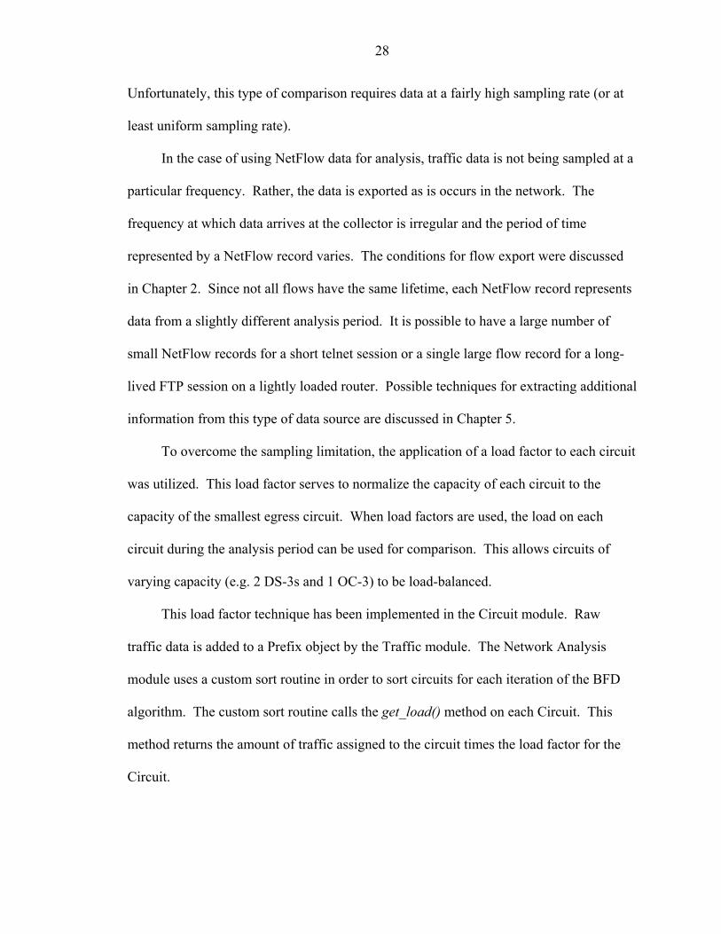
Unfortunately, this type of comparison requires data at a fairly high sampling rate (or at

least uniform sampling rate).

In the case of using NetFlow data for analysis, traffic data is not being sampled at a

particular frequency. Rather, the data is exported as is occurs in the network. The

frequency at which data arrives at the collector is irregular and the period of time

represented by a NetFlow record varies. The conditions for flow export were discussed

in Chapter 2. Since not all flows have the same lifetime, each NetFlow record represents

data from a slightly different analysis period. It is possible to have a large number of

small NetFlow records for a short telnet session or a single large flow record for a long-

lived FTP session on a lightly loaded router. Possible techniques for extracting additional

information from this type of data source are discussed in Chapter 5.

To overcome the sampling limitation, the application of a load factor to each circuit

was utilized. This load factor serves to normalize the capacity of each circuit to the

capacity of the smallest egress circuit. When load factors are used, the load on each

circuit during the analysis period can be used for comparison. This allows circuits of

varying capacity (e.g. 2 DS-3s and 1 OC-3) to be load-balanced.

This load factor technique has been implemented in the Circuit module. Raw

traffic data is added to a Prefix object by the Traffic module. The Network Analysis

module uses a custom sort routine in order to sort circuits for each iteration of the BFD

algorithm. The custom sort routine calls the get_load() method on each Circuit. This

method returns the amount of traffic assigned to the circuit times the load factor for the

Circuit.

29

Configuration Generator

The Configuration Generator module was developed to provide a solution for

implementing the results of the analysis in a network. This module is implemented in

Perl and provides an interface to accept the results of the Network Analysis module and

generate the configuration files necessary to correctly configure a router.

Benefits of Code Generation

Code generation is a technique in which programs are used to write or develop

other programs. In this case, the BGP load-balancing program generates code (or

configuration files) for a router. There are several benefits to code generation including

the reduction of human errors, standardization, and efficiency.

Though network engineers are both knowledgeable and professional, they are still

human. By developing a system that performs accurate and repeatable analysis of

network data, the network engineer can focus on other tasks that require human

intervention.

Regardless of the size of the network, standardization is a critical element of a

successful operation. By creating standard configurations and processes, networks can

scale to a very large number of elements being managed by a reasonably small staff. One

key in the operational scalability of large networks is documenting processes either in

standard, written procedures or by developing systems that establish how a particular

function should work. The Configuration Generator module encompasses what a

standard configuration should look like. Any configuration generated by this system will

be in the correct, standard format.

A goal of any system should be to improve the efficiency of the task it implements.

By automating the analysis of network traffic, BGP load-balancing can be done more

30

accurately and efficiently. It is now possible to schedule the analysis to occur at regular

intervals and store the results. This will allow an engineer to review the results and

choose the best solution to implement. To accomplish the task of analyzing network data

would be an arduous task for an engineer to perform at any reasonable frequency.

Additionally, without the traffic information being available the typical solution would

involve only an educated guess by an engineer familiar with the network.

Implementation Process

Once the analysis has been completed, an engineer must implement the

configuration. While it would be possible to extend the system to implement the

configuration in a live network automatically, that functionality is beyond the scope of

this work.

The first requirement for announcing prefixes into BGP is to configure network

statements that include all address space. To avoid issues with IGP synchronization, null

routes are also configured for each network statement. Without additional routing policy,

the network statements and null routes would generate BGP updates for the entire address

space.

With only network statements and no routing policy, all updates announced would

have the same metric. The addition of routing policy to affect load balancing is

accomplished via route-maps. Route-maps use an if-then-else type construct to allow

modifications to be made to attributes of a BGP announcement. In the case of load

balancing, the route-map has a term that matches all IP space within a prefix. For each

match, the MED value is changed to prefer the circuit or not depending on which prefix

list is matched. If the IP space falls in the prefix list for the circuit, the MED value is set

to 50 and traffic from that range will prefer the circuit. For all other space, the MED

31

value is set to 200. By using a default MED value, any IP prefix that does not have

routing policy applied will still be advertised. In the case of the failure of an egress link,

the prefixes that were preferred on the link will continue to route across other links at a

higher MED value. Without this catchall, the more strict routing policy would create an

outage for the preferred blocks when an egress link goes down.

Figure 3-1 Process by which router applies BGP routing policy via route-maps and prefix-lists.

neighbor A

route-mapRouterA

prefix-listRouterA

prefix-listIP-ALL

Router A

route-mapRouterB

prefix-listRouterB

prefix-listIP-ALL

Router B

neighbor B

networkstatements

dampening,synchronization,

etc...

Global BGPconfiguration

32

router bgp 65000 no synchronization bgp log-neighbor-changes network 10.0.0.0 mask 255.255.248.0 network 10.0.8.0 mask 255.255.248.0 network 10.0.16.0 mask 255.255.248.0 network 10.0.24.0 mask 255.255.248.0 network 192.168.80.0 mask 255.255.248.0 network 192.168.96.0 mask 255.255.248.0 network 192.168.128.0 mask 255.255.248.0 network 192.168.160.0 mask 255.255.248.0 neighbor 192.168.1.50 remote-as 1234 neighbor 192.168.1.50 description RouterA neighbor 192.168.1.50 route-map RM-RouterA out neighbor 192.168.1.100 remote-as 5678 neighbor 192.168.1.100 description RouterB neighbor 192.168.1.100 route-map RM-RouterB out

Figure 3-2 Basic BGP configuration without routing policy.

ip prefix-list IP-ALL seq 5 permit 10.0.0.0/21 ip prefix-list IP-ALL seq 10 permit 10.0.8.0/21 ip prefix-list IP-ALL seq 15 permit 10.0.16.0/21 ip prefix-list IP-ALL seq 20 permit 10.0.24.0/21 ip prefix-list IP-ALL seq 25 permit 192.168.80.0/21 ip prefix-list IP-ALL seq 30 permit 192.168.96.0/21 ip prefix-list IP-ALL seq 35 permit 192.168.128.0/21 ip prefix-list IP-ALL seq 40 permit 192.168.160.0/21 ! ip prefix-list RouterA seq 5 permit 10.0.0.0/21 ip prefix-list RouterA seq 10 permit 10.0.8.0/21 ip prefix-list RouterA seq 15 permit 10.0.16.0/21 ip prefix-list RouterA seq 20 permit 10.0.24.0/21 ! ip prefix-list RouterB seq 5 permit 192.168.80.0/21 ip prefix-list RouterB seq 10 permit 192.168.96.0/21 ip prefix-list RouterB seq 15 permit 192.168.128.0/21 ip prefix-list RouterB seq 20 permit 192.168.160.0/21

Figure 3-3 IP prefix list configuration to identify groups of prefix that will have routing

policy applied.

33

route-map RM-RouterA permit 10 match ip address prefix-list RouterA set metric 50 ! route-map RM-RouterA permit 20 match ip address prefix-list IP-ALL set metric 200 ! route-map RM-RouterB permit 10 match ip address prefix-list RouterB set metric 50 ! route-map RM-RouterB permit 20 match ip address prefix-list IP-ALL set metric 200

Figure 3-4 Route-maps use prefix-lists to apply routing policy to outbound BGP

announcements.

The system generates a route-map and prefix list for each BGP neighbor. Another

prefix-list call IP-ALL is also generated. This prefix-list includes all valid address space.

It is used to ensure that all address space is advertised out of every circuit.

CHAPTER 4 SYSTEM RESULTS

This chapter discusses testing that was conducted to validate the BGP load-

balancing system. The test setup and procedures are presented. Results and observations

from the various test cases are included. Finally, several topics for further investigation

are suggested.

Testbed Configuration

The testbed used to evaluate the system was built to mimic what a typical access

network might look like. In order to understand the lab configuration, it is important to

understand how a typical access network is configured. Figure 4-1 shows a typical

access network configuration.

In a typical network, end users are connected via an access router. This access

router could be a PPP aggregator in a DSL network, Cable Modem Termination System

(CMTS) in cable modem networks, or access point in wireless networks. This layer is

where per-subscriber configuration is done. This configuration can include subscriber

authentication, rate-limiting, and IP address assignment.

In order to simulate end users in the lab setup, IP pool interfaces were configured in

the access router. One interface for each /24 subnet used in the testing was configured.

These interfaces would be the default gateway that end users would be assigned in a

production network.

34

35

Access Router

Core Router

End Users

Internet

Figure 4-1 A typical access network configuration.

Eight subnets were utilized for the testing. The subnets are contained in Table 4-1.

These subnets are initially configured as IP prefixes with a 21 bit subnet mask. The

subnets are only split if the Network Analysis module identifies the subnet as a large

portion of the traffic.

Traffic Generation

During testing of the traffic collection module, the test setup shown in Figure 4-2

was used. The ping command was used to send ICMP traffic into the network from a

Unix workstation. Command line options allow a user to specify both the number of

36

packets as well as packet size. This allows for a user-defined amount of ICMP traffic to

be sent to a single IP address.

Table 4-1 Subnets that were utilized during lab testing.

IP prefix Subnet mask 10.0.0.0 255.255.248.0 10.0.8.0 255.255.248.0 10.0.16.0 255.255.248.0 10.0.24.0 255.255.248.0 192.168.80.0 255.255.248.0 192.168.96.0 255.255.248.0 192.168.128.0 255.255.248.0 192.168.160.0 255.255.248.0

Figure 4-2 Lab setup used to test BGP load-balancing tool.

---------------------------------------------------------------------------------------------------------------------------------------------------------------------------------------------------------------------------------------------------- --Cisco 7200Series

3

1

4

2

0

1 2 3 4 1 2

3 4

1 2 3 4 1 2 3 4

1 2 3 4

5 6 7 8

5 6 7 8

1 2 3 4

SD

ENAB LE

D

SLOT 0

PCMC IA

EJEC

T

FE M II

AUI

ENAB

LEFE

FE LI

NK

E NABL

E

CPU R

ST

IO P

OWER

OK

SD

P OWER READY ALARM

FA IL STAT RUN RESETENET

CLAS S 1LA SE R

PRODUCT

151413121110987643210 5

CONS OLE 1

C I S C O Y S T E MS

Cisco 7206

Cisco 7206

RedbackSMS1800

Cisco 7500 SERIES

NORMALLOWERPOW ER

UPPERPOWER

Traffficgenerator

--------------------------------------------------------------------------------------------------------------------------------------------------------------------------------------------------------------------------------------------------- --Cisco 7200Series

3

1

4

2

0

1 2 3 4 1 2

3 4

1 2 3 4 1 2 3 4

1 2 3 4

5 6 7 8

5 6 7 8

1 2 3 4

SD

ENABL

ED

SLOT 0

PCMC IA

E JECT

FE M

I I

AUI

E NABL

EFE

F E L IN

K

ENAB

LE

CPU R

ST

IO P

OWE R

OK

SD

0 1 2 3 4 5 6 7 1 0 Powe r 1 Po wer 21 4 15 16

ESD

8 9 1 1 12 13

ks

--------------------------------------

C IS CO YS TEM SS

FAST ETHERNET INPUT/OUTPUT CONTROLLER

---------------------------------------

C ISCO Y STEMSS

FAST ETHERNET INPUT/OUTPU T CO NTROLLER

Re dBac k Networ

37

This method was used to test the traffic collection module and its ability to decode

and s

is study. The

analy n

s

Several test cases were developed to test the ability of this system to generate load-

balan

l

ses considered in this study are shown in Table 4-2. Each case is explained

in fur

ring validation testing.

tore NetFlow records. Additional testing was conducted by generating SQL code to

populate the database with traffic information directly. This allowed for the creation and

execution of tests cases without utilizing the traffic collection module.

There was no consideration for type or distribution of traffic in th

sis module balances based on aggregate load values. The specific type or duratio

of each flow has little meaning in this approach.

Test Case

ced BGP configurations. The cases considered include both well-balanced and

unbalanced traffic conditions. This tested the performance of the system under norma

network conditions (nearly balanced) as well as worst-case conditions (significantly

unbalanced). Test case #4 also included load balancing across circuits with different

capacities.

The ca

ther detail in the following sections.

Table 4-2 Description of test cases used du

Case Id Test Case 1 Even distribution ross all prefixes of traffic ac2 Even traf 1 prefix fic in 2 /24 prefixes that fall within the same /23 Random distribution of traffic across all prefixes

4 Random distribution of traffic across all prefixes with unequal size circuits

38

System Output

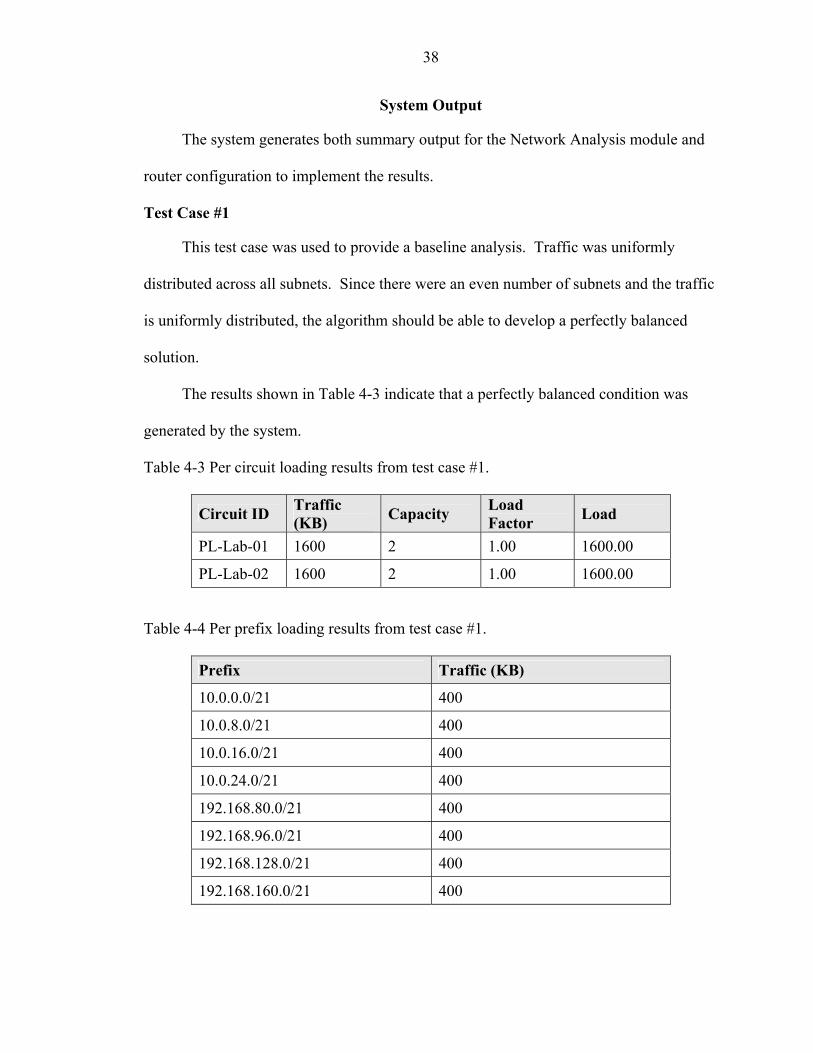
The system generates both summary output for the Network Analysis module and

router configuration to implement the results.

Test Case #1

This test case was used to provide a baseline analysis. Traffic was uniformly

distributed across all subnets. Since there were an even number of subnets and the traffic

is uniformly distributed, the algorithm should be able to develop a perfectly balanced

solution.

The results shown in Table 4-3 indicate that a perfectly balanced condition was

generated by the system.

Table 4-3 Per circuit loading results from test case #1.

Circuit ID Traffic (KB) Capacity Load

Factor Load

PL-Lab-01 1600 2 1.00 1600.00

PL-Lab-02 1600 2 1.00 1600.00

Table 4-4 Per prefix loading results from test case #1.

Prefix Traffic (KB)

10.0.0.0/21 400

10.0.8.0/21 400

10.0.16.0/21 400

10.0.24.0/21 400

192.168.80.0/21 400

192.168.96.0/21 400

192.168.128.0/21 400

192.168.160.0/21 400

39

Test Case #2

The purpose of this test case was to evaluate how well the system performed with a

highly skewed traffic distribution. The case was derived so that two prefixes had an

identical amount of traffic. These two subnets were chosen such that they fell within the

same /23 supernet. With this arrangement, a perfectly balanced configuration was

possible but would require several iterations of the algorithm to achieve.

Table 4-5 shows that the ideal balanced condition was generated using 11 prefixes.

This indicates that there were 4 iterations of the algorithm. The skewed distribution of

traffic is visible in Table 4-6.


Circuit ID Traffic (KB) Capacity Load Factor Load

PL-Lab-01 50 2 1.00 50.00

PL-Lab-02 50 2 1.00 50.00


Prefix Traffic (KB) 10.0.0.0/24 50 10.0.1.0/24 50 10.0.2.0/23 0 10.0.4.0/22 0 10.0.8.0/21 0 10.0.16.0/21 0 10.0.24.0/21 0 192.168.80.0/21 0 192.168.96.0/21 0 192.168.128.0/21 0 192.168.160.0/21 0

40

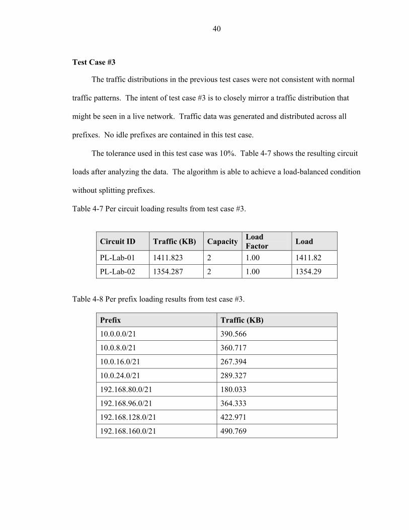
Test Case #3

The traffic distributions in the previous test cases were not consistent with normal

traffic patterns. The intent of test case #3 is to closely mirror a traffic distribution that

might be seen in a live network. Traffic data was generated and distributed across all

prefixes. No idle prefixes are contained in this test case.

The tolerance used in this test case was 10%. Table 4-7 shows the resulting circuit

loads after analyzing the data. The algorithm is able to achieve a load-balanced condition

without splitting prefixes.



PL-Lab-01 1411.823 2 1.00 1411.82

PL-Lab-02 1354.287 2 1.00 1354.29


Prefix Traffic (KB)

10.0.0.0/21 390.566

10.0.8.0/21 360.717

10.0.16.0/21 267.394

10.0.24.0/21 289.327

192.168.80.0/21 180.033

192.168.96.0/21 364.333

192.168.128.0/21 422.971

192.168.160.0/21 490.769

41

Test Case #4

A slightly more complicated scenario is presented in test case #4. This case used

randomly distributed traffic across all subnets. The tolerance for determining balance

condition was lowered from 10% to 5%. Additionally, circuit #2 has twice the capacity

of circuit #1. This validates that the concept of balancing traffic on load rather than

traffic works correctly.



PL-Lab-01 1077.613 2 1.00 1077.61

PL-Lab-02 2091.995 4 0.50 1046.00


Prefix Traffic (KB)

10.0.0.0/21 419.265

10.0.8.0/21 260.42

10.0.16.0/21 383.099

10.0.24.0/21 397.928

192.168.80.0/22 296.812

192.168.84.0/22 197.234

192.168.96.0/21 404.345

192.168.128.0/21 358.856

192.168.160.0/21 451.649

Conclusions

The test results discussed in this section demonstrate that the system for generating

load-balanced BGP configurations works correctly. Scenarios that required prefix

42

splitting were included to test the algorithms ability to generate a new set of initial

conditions that could be used in the next iteration to develop a better solution.

The test cases that used random data spread across all prefixes are a more accurate

representation of real world traffic. In these test cases, the system was able to achieve a

load-balanced condition under both 5% and 10% tolerance settings. With the variations

in traffic levels in live networks, these thresholds are reasonable.

Regardless of the complications added to each test case, the system was able to

achieve the desired result. Balanced BGP configuration can be developed in an

automated fashion by analyzing traffic data and network topology.

CHAPTER 5 SUMMARY AND FUTURE WORK

The system developed in this study is a proof of concept implementation to show

that load-balanced configurations can be developed through network analysis. This

chapter discusses some improvements to the system as well as some opportunities for

enhancement that can be realized by implementing this type of system.

System Improvement

During the development of this system, several issues were discovered that might

cause the system to provide less than ideal results. The following sections outline these

issues and propose solutions to the underlying problems.

Instantaneous Data Rate Load-Balancing

The load-balancing done in this system is based on aggregate load during an

analysis period. The goal is not to ensure that the instantaneous data rate on each circuit

is balanced at some peak time. Rather, the system ensures that the total flow of traffic

out each circuit during the entire analysis period is equal. The calculation is more a

balance of volume than of rate.

The reason that using a volumetric method is appropriate is that network traffic

patterns are regular on a day-to-day basis. Peak traffic levels tend to increase in a linear

fashion over time. The traffic patterns are somewhat predictable. These patterns are

illustrated in Figure 5-1.

43

44

While the total volume of traffic is fairly predictable, what is not predictable is

which subnets will originate the traffic. Because end users are assigned IP addresses out

of one of several pools, it is common for dynamic users to change IP addresses.

Figure 5-1 Total volume of traffic is predictable on a day-to-day basis and grows linearly over time.

In order to balance traffic on an instantaneous data rate basis, the NetFlow data

must be discretized. Data must be sampled on a small interval. The flow records contain

an aggregate amount of data during a period of time. The period represented by each

flow record is different. Each datum from a flow record is assigned to the timeslot during

which it was generated.

Since the information in a flow record spans many timeslots, some assumptions

must be made about the distribution of data during the flow record’s interval. In order to

make this type of assignment, several challenges must be overcome:

• The flow distribution models must be developed for each protocol present in the network.

• The protocol contained in the flow must be determined from the information contained in the NetFlow record. (i.e., non-standard ports would skew the results)

• The sampling interval must be smaller than most of the flow records.

45

Although not impossible to solve, these problems are beyond the scope of this

thesis. When considering the traffic characteristics presented earlier in this section and

the difficulty in extracting additional information from the flow records, the system

described in this paper is a good trade-off between accuracy and complexity.

Low Utilization Prefixes

Because the load-balancing system makes prefix assignments based on load, the

presence of low or zero utilization prefixes have little impact on these assignments. This

can lead to router configurations where the load is perfectly balanced but the number of

IP addresses assigned to each egress link is drastically different. This was exhibited in

the configurations generated by test case #2 shown in Figure 5-2. The prefix lists are

balanced based on current load, but the number of addresses on each circuit are not

balanced.

If left unchecked, this issue could result in the configuration being significantly out

of balance as these subnets become utilized. In order to alleviate this problem, another

analysis pass could be performed that would use the load-balanced configuration as the

initial condition. This algorithm would look for low or zero utilization prefixes and

balance them across the links based on the number of IP addresses in the prefix. After

this pass, the configuration would represent a current load-balanced state as well as

balancing the number of addresses thereby extending the period of time that this

configuration will maintain load-balance.

46

ip prefix-list IP-PL-Lab-01 description Networks preferred on Circuit ID PL-Lab-01 ip prefix-list IP-PL-Lab-01 seq 5 permit 10.0.1.0/24 ip prefix-list IP-PL-Lab-01 seq 10 permit 10.0.8.0/21 ip prefix-list IP-PL-Lab-01 seq 15 permit 10.0.16.0/21 ip prefix-list IP-PL-Lab-01 seq 20 permit 10.0.24.0/21 ip prefix-list IP-PL-Lab-01 seq 25 permit 192.168.80.0/21 ip prefix-list IP-PL-Lab-01 seq 30 permit 192.168.96.0/21 ip prefix-list IP-PL-Lab-01 seq 35 permit 192.168.128.0/21 ip prefix-list IP-PL-Lab-01 seq 40 permit 192.168.160.0/21 ip prefix-list IP-PL-Lab-01 seq 45 permit 10.0.4.0/22 ip prefix-list IP-PL-Lab-01 seq 50 permit 10.0.2.0/23 ip prefix-list IP-PL-Lab-02 description Networks preferred on Circuit ID PL-Lab-02 ip prefix-list IP-PL-Lab-02 seq 5 permit 10.0.0.0/24

Figure 5-2 System generated prefix lists are balanced based on load, but not necessarily balanced on number of addresses.

Minimizing Prefix Announcements

Another issue that exists in the current tool is that the number of prefixes is

expanded so that a load-balanced condition can be reached. This can lead to a

configuration whereby after several iterations, two subnets that belong to the same

supernet are assigned to the same circuit. In this case, the two subnets could be collapsed

into a single prefix announcement for the supernet.

Scanning each circuit after the analysis and looking for adjacent prefixes could

resolve this issue. This technique would be simple to implement and would have O(n)

complexity.

Cost Factor in Load Balancing

Including the cost of bandwidth into the load-balancing calculation is potential area

for exploration. This study had no preference as to which egress circuit should be

utilized first. Dual-homed configurations increase redundancy and reliability of BGP

47

peering. In a dual-homed configuration, a network operator obtains egress links from

multiple providers to ensure that they are protected from a failure in the service provider

network. To reduce the cost of this type of configuration, the backup link can be on

usage based billing or burstable billing. In usage based billing, the customer pays based

on how much bandwidth they utilize. In a burstable billing scenario, the customer pays

for a certain amount of bandwidth. If they exceed the allocated bandwidth, they pay a

higher rate for the additional capacity.

These factors could be included in the algorithm by modifying how the circuits are

sorted during the iterations of BFD. Rather than sorting just on load, the sort method

would include both the load on the circuit and the cost of exceeding the threshold for

burstable circuits. Usage base circuits could be handled by the same method with a zero

threshold.

Support More Complicated Route-Maps

Route-maps are utilized in this system to apply the load-balanced routing policy to

BGP announcements. This is the type of route-map term supported.

Other types of routing policy are also implemented through route-maps. This

system could be adapted to include other routing policy terms present in the route-map

prior to analysis. This would integrate the existing routing policy with the changes

required to maintain load-balance.

This type of change would require parsing of the existing configuration file or

additional changes to the database to include routing policy beyond the scope of load-

balancing.

48

Fault Detection

The data available in this system would allow for the development of some

additional fault detection capabilities. By mapping traffic data to egress links, over-

utilization conditions on egress circuits can be identified. This type of information can

typically be obtained by other means (e.g., SNMP).

The ability to break down the traffic information from an overloaded circuit to a

more granular level is an enhanced capability. Once an issue has been identified, the

traffic data will indicate what type of services are consuming the link and what hosts are

the source of that traffic.

Infected Host Detection

One specific example of fault detection is infected host detection. The data

gathered for load balancing will include signs of virus presence or propagation. Not all

viruses and worms could be detected, but many have signatures that can be identified by

looking at flow characteristics. Also, host enumeration would be detected in this case.

Enumeration might involve ICMP and port scanning to identify hosts where a worm can

propagate.

Summary

The goal of this project was to develop a system that could analyze network traffic

and generate load-balanced router configurations. The motivation for this effort is that

the existing process today is manual, intensive, and potentially error prone.

Today, an engineer must evaluate load conditions on each egress link within an AS.

Aggregate traffic levels on a per-circuit basis and the number of IP addresses preferred on

each link is the only information that the engineer has available. The engineer

49

determines an estimate of how much traffic needs to be moved. The step is based on

estimation and can lead to errors.

This system analyzes data and assigns traffic at an IP prefix level. This allows for

accurate determination on how much traffic will migrate when the preference on a

particular IP prefix is adjusted. This eliminates the guesswork and estimation in today’s

process.

Rather than simply identifying a prefix to move, the system analyzes the entire

system and develops a new set of prefix to circuit assignments that achieves a well-

balanced state. This analysis is based on data across all IP prefixes. The system has been

shown to be effective across a range of cases that test both normal traffic conditions as

well as irregular traffic that represent challenges for the algorithm.

The enhancements presented in this chapter are by no means complete. There are

certainly additional features that could be developed that would allow this system to play

an integral role in a network management suite.

LIST OF REFERENCES

Argawal S, Chuah C, and Bhattacharyya S, Diot C, 2004, “The Impact of BGP Dynamics on Intra-Domain Traffic,” Proceedings of the Joint International Conference on Measurement and Modeling of Computer Systems, ACM Press, pp. 319-330.

Bressoud T, and Rastogi R, “Optimal Configuration for BGP Route Selection,” INFOCOM 2003: Twenty-Second Annual Joint Conference of the IEEE Computer and Communications Societies, Vol. 2, pp 916-926

Christiansen T, and Torkington N, 1999, Perl Cookbook, O’Reilly & Associates, Inc, Sebastopol, CA.

Halabi B, 1997, Internet Routing Architectures, Cisco Press, Indianapolis, IN.

Holzner S, 1999, Perl Core Language, Coriolis Technology Press, Scottsdale, AZ.

Horowitz E, Sahni S, and Rajasekaran S 1998, Computer Algorithms, Computer Science Press, New York, NY.

Nilsson S, and Karlsson G, 1999, “IP-Address Lookup Using LC-Tries,” IEEE Journal on Selected Areas in Communication, Vol. 17, No. 6, pp 1083-1092.

Lili Q, Zhang Y, and Keshav S. "Understanding the Performance of Many TCP Flows," Computer Networks (formerly called Computer Networks and ISDN Systems), Vol. 37, pp 277-306, 2001.

Sahni, Sartaj, 2000, Data Structures, Algorithms, and Applications in Java, McGraw-Hill, Boston, MA.

Savelsbergh M, 1997, “A Branch-and-Price Algorithm for the Generalized Assignment Problem,” Operations Research, Vol. 45, No. 6, pp 831-841, 1997.

Sklower K, 1991, “A Tree-Based Packet Routing Table for Berkeley Unix,” Proceedings of the 1991 Winter USENIX Technical Conference, Dallas, TX, pp 93-99.

Stallings W, 2000, Data and Computer Communications, Prentice Hall, Sixth Edition, Upper Saddle River, NJ.

Tanenbaum A, 1996, Computer Networks, Prentice Hall, Third Edition, Upper Saddle River, NJ.

50

BIOGRAPHICAL SKETCH

I received a Bachelor of Science degree in civil engineering from the Florida State

University in 1997. During my undergraduate studies, I was employed by Post, Buckley,

Schuh, and Jernigan (PBS&J) and at the Florida Department of Transportation Structural

Research Center. This practical, hands-on engineering experience proved beneficial

during my graduate studies.

I began my graduate school career under Dr. Peter Ifju in the Aerospace

Engineering, Mechanics and Engineering Science (AEMES) Department at the

University of Florida in 1997. I studied the post-buckling response of composite

sandwich structures and published a thesis on the topic.

My studies in the Computer and Information Science and Engineering (CISE)

Department at the University of Florida began while writing my thesis in aerospace

engineering. During my tenure in computer engineering, I have focused on network

communications and security. Both my academic progress and network-related research

are represented by this thesis. This thesis was defended on October 6th, 2004.

51

AUTOMATED SYSTEM FOR LOAD-BALANCING EBGP...

Documents

Transcript of AUTOMATED SYSTEM FOR LOAD-BALANCING EBGP...