Automated Software Size Estimation based on Function Points using UML Models

Aleš Živkovič, Ivan Rozman, Marjan Heričko

University of Maribor, Faculty of Electrical Engineering and Computer Science,

Smetanova 17, SI-2000 Maribor, Slovenia Phone: +386 2 235 5115, e-mail: ales.zivkovic@uni-mb.si

Abstract A systematic approach to software size estimation is important for accurate project planning. In this paper, we will propose the unified mapping of UML models into function points. The mapping is formally described to enable the automation of the counting procedure. Three estimation levels are defined that correspond to the different abstraction levels of the software system. The level of abstraction influences an estimate's accuracy. Our research, based on a small data set, proved that accuracy increases with each subsequent abstraction level. Changes to the FPA complexity tables for transactional functions will also be proposed in order to better quantify the characteristics of object-oriented software. Keywords: function points, software size measure, project planning

1 Introduction The focus of scientific research regarding object development and component-based development has already shifted from implementation to earlier development activities in software and information system development. Additionally, emphasis has also been placed on all aspects of software development that have been investigated in the context of structured techniques, from executable specifications, testing strategies to estimation models and metrics. In this paper, we will focus on one metric only: the size estimation metric for object-oriented development. Software size contains important information for project planning. Costs and schedule estimates depend on its existence and its accuracy; indirectly the project's success also depends on it. A software project is successful if the requirements are fulfilled and no budget or deadline overflows occur [25]. With systematic size estimation, the risk of overflows is lower. Systematic software size estimation requires a method that defines a procedure for measurement, involving units and accuracy. In general, Functional Size Measurement (FSM) methods, as defined in ISO/IEC TR 14143 [12, 13, 14, 15] can be categorized into two groups. In the first group, there are technology-independent methods; an example would be the Function Point Analysis (FPA) method [10]. In the second group, there are technology-dependent methods; for example Lines of Code (LOC) or number of classes. The methods from the first group have obvious advantages over the methods from the second group. The ultimate goal is to use only technology-independent methods. The FPA method dates back to 1979 [2] and has been updated several times. However, the core concepts and the counting procedure remains the same. Every information system processes some data that can be stored in the application database or is taken from external applications. Four operations are performed on data records: create, read, update and delete. Besides that, information systems use several query functions for data retrieval and report construction. Each record consists of several fields of basic data types or another record that can be further deconstructed. The FPA method quantifies: the number of fields in each record, the distinct

operations performed on these records, and the number of these operations that are necessary to perform a business function. The sum over all business functions, multiplied with some empirically determined weights, represents the unadjusted function points value. The final calculation is made using a Value Adjustment Factor (VAF) that measures system complexity. Based on the FPA method, several methods like Feature points, Full Function Points, Function Weight, Function Bang, Mk II Function Points Analysis, COSMIC-FFP and NESMA evolved. A detailed comparison of the selected methods can be found in [33]. Although the methods are technology-independent, their use in object development is quite difficult. Methods use their own abstraction to represent a software system in a convenient way, so as to perform size count. In object development, the Unified Modeling Language (UML) is used to represent the software system as an abstraction. To overcome the gap between these two abstractions, the mapping that transforms the elements used in one abstraction to the elements of the other abstraction, has to be defined. This paper focuses on OO-to-FPA mappings. With OO-to-FPA mapping defined, the late analysis and design size estimation problem is solved, however the estimation cannot always be applied early in a software development process. To perform an early estimate, historical data are needed to fulfill the missing information with some statistical function. The fact is that the early estimates are far more valuable than the estimates in design time, but difficult to acquire in desired accuracy. In our approach, the statistical approach is used. This paper is divided into five sections. In the next section, the importance of size estimation is emphasized, the FPA method is briefly described, and a detailed review of the literature is given. In the third section, different OO-to-FPA mappings are described and compared. Based on the results, a new, unified OO-to-FPA mapping is proposed in section four, together with several additional improvements that address current size estimation problems. The problem of inaccuracy in early estimates is addressed with the aid of different estimation levels. Section five summarizes the results of the improvements that were introduced into the size estimation process for object-oriented projects and also discusses further improvements.

2 Related work The research community found several problems related to the FPA method. These problems can be grouped together by their research area:

1. Correlation between FPA elements [17,18,20]. 2. Inappropriate formulation of the VAF and the General System Characteristic (GSC)

[21]. 3. Informal definition and violation of monotony [1,6,7]. 4. The gap between OO and FPA abstractions [3,4,5,8, 27, 31].

Lokan [20] analyzed 269 projects and tried to discover the correlation between five elements used in the FPA method to represent a software system. He found out that External Inputs (EI) and Internal Logical Files (ILF) always correlate, while External Interface Files (EIF) rarely correlate with other elements. Another paper [21] analyzed 235 projects with an emphasis on GSC. The research was divided into two parts. In the first part, Lokan proved that GSC is out-of-date and not appropriate for today's systems. In the second part, he used empirical analysis to show that 14 technical factors were not independent and expressed overlapping characteristics. Therefore, the smaller set could be used instead. The research also showed that VAF improved the estimated size in less than half of all cases. All methods for software size estimation lack adequate formal foundations in their origin descriptions. There were some attempts [6,7] to add formality to functional size measurement.

Fetcke's model is applicable to different methods since it introduced an additional level of abstraction, called a data-oriented abstraction. The approach proposed by Diab et al. was designated COSMIC-FPP [35] and had a specific purpose. In our research, the model defined by Fetcke is used as a basis and further refined by the definition of a mapping function [33]. The abstraction is also used to formally describe an OO-to-FPA transformation, as proposed in this paper. The violation of monotony first addressed in MK II FPA [30], later formally proven by Fetcke [6] and again addressed in research [1] resulted in a change in complexity weights. Since our research also resulted in a change of complexity tables different from the one proposed by [1], this approach is discussed in more detail. In Al-Hajri's research, tables gathered with the training methods from Neural Networks replaced the original complexity tables. The results showed that the average error decreased and the convergence between actual effort and estimated effort improved. The authors extended complexity tables and related ordinal scales with absolute ones. However, the new tables are not appropriate for our research since we deal with object-oriented systems that have specific characteristics. These characteristics will be presented in the next section. We believe that Al-Hajri's approach could also be used to further improve our tables. Unfortunately, at the moment there is not enough empirical data available in the ISBSG repository [11] to apply his procedure of weights validation.

3 OO-to-FPA mappings 3.1 Method proposed by Fetcke, et al. Fetcke et al. [8] focused their research on a specific method, namely Object-Oriented Software Engineering (OOSE) [16]. This method is based on use cases. The authors proposed four groups of rules:

• Identification of the counting boundary. • Identification of items within the boundary (transactional and data functions). • Identification of the item type (Data Element Type, DET; Record Element Type, RET;

File Type Referenced, FTR) for all items. • Prescribing the weight factors.

The application boundary is set in accordance with the definition of the boundary in the Use Case (UC) diagram, as defined in the UML standard. Actors are mapped into users of the system. Use Cases are mapped into transactional functions. This mapping is not always one-to-one. The number of transactional functions for the particular UC is usually defined by the UC description. The authors do not provide additional guidelines on the matter. The reference to the rules of the original method is noted. Since the OOSE method distinguishes between three types of objects (control, entity and boundary), only entity objects and objects with unknown types performing a count at the time, are used as data functions. Aggregation and generalization are treated in a specific way. Both concepts can have a significant impact on the number of data elements types, record element types and file types referenced, respectively. 3.2 Method proposed by Uemura, et al. Uemura et al.[28,29] use class and sequence diagrams as sources for OO-FPA mapping. The mapping is specified for diagrams developed in design that conduct design specification. The system boundary is identified according to the messages in the sequence diagrams. The messages sent by actors to non-actor objects represent the system boundary. Basically, the rule is the same as defined in the UML standard [23], the only difference is the diagram from

which the boundary is identified. We can simplify this rule to become consistent with the rule used by Fetcke et al.[8]. Under the presumption that each sequence diagram is directly related to one UC in the UC diagram, the boundary can be identified from the UC diagram. Objects with at least one attribute that have one or more methods or call methods of other objects are mapped into data functions. The classes with methods that influence the state of other objects are mapped to external interface files (EIF). All others are considered internal logical files (ILF). Transactional functions are identified according to five different communication patterns from the sequence diagram. The transactional function type is also identified from the communication pattern. 3.3 Method proposed by Antoniol, et al. Antoniol et al. [3,4,5] propose two methods for estimating size during the development process. In the early project phase, the use of the original FPA method is suggested. After the design is conducted, a method developed by the authors, called Object-Oriented Function Points (OOFP), is considered to be the most appropriate. The OOFP method is based on the deliverables of the design phase and takes advantages of the information available in the class diagrams. With this method, the gap between the system abstraction (used by the FPA method) and the abstraction made with class diagrams is supposed to be resolved. The method provides additional rules and allows some freedom of choice for the mapping algorithm, in cases where class diagrams exhibit complex class hierarchies. The number of attributes and associations with other classes are used to define internal logical file complexity. To distinguish between data element types and record element types, a simple but indistinct rule is used. The complex data types are classified as record element types, while simple or primitive data types are classified as data element types. Transactional functions are identified according to the methods in the class. The authors call them service requests. Abstract methods and inherited methods are ignored. Method complexity is determined according to the number of parameters and global variables referenced in the method. As is the case with attributes, the element data type is used for the classification of data element types, or the file types referenced. 3.4 Method proposed by Ram, et al. The mapping is basically the same as in the OOFP approach. The function points for each class are calculated. The number of function points for the class is a sum of its logical file and transactional functions contribution. The transactional functions contribution is calculated from the methods; whereas for methods without parameters and with the void return type, complexity is considered as if it were for one DET. Ram and Raju [26] define additional rules for class complexity classification. These rules are used in the second step. Class complexity is defined as being low if the class processes less than 50% of data visible to the class, average if 51 to 70% is processed, and high if the amount of processed data exceeds 70%. A numerical value is then assigned to the given complexity and multiplied with the number of function points calculated in the first step. The final amount is lowered by 10, 40 or 70 percent, depending on its complexity. The term "data elements which are visible to all methods of a class" used by Ram and Raju [26] is uncommon since such data elements are called attributes and are by definition visible in all methods. The term "process the data" is also weakly defined. Do the get and set methods process the data? If the answer is yes, then the second step concept fails, otherwise it is difficult to automate steps, since a deep insight into the method's behavior must be considered.

3.5 Comparison of mappings Comparing all four mappings we can conclude that [8] and [28,29] define "boundary" in the same way. Fetcke et al.[8] uses UC diagrams as a reference for boundary identification, Uemura et al.[28, 29] uses sequence diagrams. Conceptually, the mappings are the same. However, from our point of view, Uemura's approach is less applicable for two reasons:

• Sequence diagrams are usually made in combination with a UC. It is uncommon to draw only sequence diagrams. However, it is not necessary for the sequence diagram to have an actor (e.g. associations "include" and "extend"). On the other hand, one UC can have many sequence diagrams that aggravate boundary identification. From the UC diagram, the boundary is directly visible and clearly defined by the UML standard.

• In the design time, it is usually clear what is in the system and what is outside it.

Classes represent the abstraction of the system to be built and are inside the fictive boundary of the system. In fact, setting the boundary at the design time is unnecessary. Thus, it does not influence further steps. Antoniol et al.[3,4,5] and Ram et al. [26] choose the same approach.

All approaches are unified in their view of data function mapping. The class is mapped to a logical file. However, the definitions for separation on internal or external logical files are weak in all four methods. Uemura et al. [28,29] uses supplemental rules to distinguish between two data element types using class operations. Antoniol et al. [3,4,5] retain the original guidelines regarding logical files division. In the OO systems, external classes encapsulate non-system components, such as other applications, external services and reused library classes. External classes correspond to external logical files, according to Antoniol et al.[3,4,5]. However, a precise definition on how to count external classes is missing. Ram and Raju [26] uses Antoniol's definition. In mappings for transactional functions, the gap between approaches is greater. Fetcke et al.[8] defines transactional functions according to the UC and their description. Uemura et al.[28,29] defines five interaction patterns. Transactional functions are recognized from the sequence diagrams according to the type of the object starting and completing the interaction sequence. Patterns are used to identify transactional function complexity. Antoniol et al. [3,4,5] uses the term “service request” instead of method, although the methods are actually counted and mapped into transactional functions. Abstract and inherited methods are not counted. In Antoniol's opinion, it is impossible to determine the type of transactional function from the class diagrams. The complexity table for external inputs and queries is used. Ram and Raju [26] also use methods to determine the number and complexity of transactional functions. When comparing his approach with Antoniol's, it can be noted that Ram and Raju [26] are more careful with inherited methods. If the inherited method overrides a method, its complexity is considered for that derived class alone. Ram and Raju [26] also point out that abstract methods are defined in the derived classes and should be considered when calculating the complexity of each derived class. Antoniol et al. [5] indirectly uses the same rule, although he does not formulate it. Ram and Raju [26] calculate the complexity of transactional functions in two steps. For the first step, they use Antoniol's approach of using a method's signature to determine its complexity contribution. In the second step, Ram and Raju [26] use its unique class complexity classification (see section 2). Antoniol et al.[3,4,5], Ram and Raju [26] and Fetcke et al.[8] pay regard to different kinds of associations that can map to either data element types or record element types/file types referenced. The rules are different. Only Uemura et al.[28,29] set the number of record element types to one for all cases.

Since compared mappings use identical transformations for the main OO concepts, it is reasonable to define a unified OO-to-FPA mapping. In the next section, one of the proposed improvements is the unification of the mapping and its formalization in such a way that size estimation can be automated using UML artifacts.

4 Proposed improvements In the previous section, four different mapping approaches were described and compared. In this section, improvements to the approaches described above are presented. The improvements are:

1. Adaptation of the ISBSG statistical approach to early estimates for use cases. 2. Unified OO-to-FPA mapping. 3. A new complexity table that better captures the characteristics of object development. 4. A formal description of the mapping rules. 5. An integrated approach to size estimation in object development

The aim is to solely use UML diagrams and cover all development phases -- not only late analysis and design. Therefore, Fetcke's idea to use UC diagrams for early estimates is supplemented with a semi-formal description of use case scenarios and integrated with an ISBSG approach to early estimates, which is based on statistical data [11]. This approach estimates software size based on deficient data, replacing the missing information with statistically proven relations between the FPA elements. In our approach, the use cases are supposed to be described with activity diagrams. Each activity in the swimlane named system is counted as one transactional function. The early estimate of software size (FPC) is calculated according to the equation E1.

TFRWNFPC TFTF ∗= (E 1)

where: • FPC is software size in function points

is the total number of transactional functions for all use cases • NTF

• TFR is the statistically acquired ratio between transactional functions and other FPA elements using the ISBSG repository or our own historical data • W is the average weight for transactional functions calculated from original FPA tables TF For more detailed estimates, class diagrams are used. We decided to use Antoniol's [3,5] mapping, change complexity tables as proposed in [4,26] and simplify the transformation procedure. The simplifications made in this research used a single class strategy [5] for identifying logical files and complexity tables that ensure minimal errors resulting from a mixture of FPA elements [33]. Some may argue that class diagrams become available late in an analysis and that no actual improvement regarding information in other diagrams is made. However, with a detailed analysis of all UML diagrams we found that the information in sequence diagrams were identical to classes together with responsibilities in the class diagram. For the function point counting procedure, the statechart diagram just supplements information about class responsibilities. Therefore, from the OO-to-FPA mapping perspective only elements in the class diagram need to be mapped. From the counting procedure’s point-of-view, additional rules are needed to define the procedure of information extraction from

sequence, statechart and activity diagrams. The definition of additional rules is beyond the scope of this paper. According to [5], OO-to-FPA mapping requires a change in complexity tables. We propose the use of Table 1 for transactional functions. The table is based on an OO metrics data analysis [9,22]. The metrics of interest are the average methods per class and average number of parameters per method. In the table, values for the number of DETs and FTRs are lowered to reach the same complexity. In object-oriented development, the number of parameters per method is usually lower than the values in the original FPA tables. To ensure results comparable to those produced by the FPA method, the linearity problem of the weights was deliberately left unsolved. This problem can be solved using several different approaches [1,19]. The size estimation results using a changed complexity table (see Table 1) can be found in the method evaluation section. 4.1 Mapping formalization In this section, a procedure for counting function points based on UML artifacts is formalized using data abstraction as defined in [7, 33]. The system is composed of different data and transactional types. The number of data and transactional types, and their attributes, contribute to the size of the software system. Some methods also define a third component that has an influence on software size -- the technical complexity of the solution. The universal function that maps application attributes into size is therefore:

)()()()( 321 TCFPCfFPCtFPCaFPCj

ji

i ∗⎟⎟⎠

⎞⎜⎜⎝

⎛+= ∑∑

(E 2)

where: • FPC(a) is the function that maps attributes of application a into software size, expressed in function points. • FPC (t ) is the function that maps transactional type t into size. 1 i i

• FPC (f ) is the function that maps data type f into size. 2 j j

• FPC3(TC) is the function that maps technical complexity of the anticipated solution for application a into a factor. The total value for an application size is the sum of FPC and FPC1 2 multiplied by the factor of the solution’s complexity. The factor can reduce or increase the overall size. However, it is not clear if the factor actually measures raw application size or is an attribute of the implementation and should be part of the function that maps size to effort. In this research, the function of FPC3 was not examined. FPC functions for our approach are presented by the equation E3.

10)(11)(

_0)(_1)(

)()(

)()(

),(

1

1

11

2

≠⇒=

=⇒==⇒=

=⇒=

+=

+=

=

−

−

−− ∑∑

∑∑

tymultiplici

tymultiplici

lkg

lkd

gdILF

llOllO

typesimpleppStypecomplexppS

lOkSN

lOkSN

NNWFPC

typecomplexppStypesimpleppS

pSN

pSNNNWFPC

pr

pd

rdEI

_0)(_1)(

)(

)(),(

1

1

=⇒==⇒=

=

=

=

∑

∑−

(a) (b) E 3

In equation E3, the functions WEI and WILF transform descriptive element complexity to the number of function points in accordance with the original FPA tables and the changed table (Table 1). Function W has two parameters. For transactional functions, those parameters are the number of data elements (N ) and the number of file types referenced (Nd r). The values for N , Nd r and Ng are determined once for each class from a corresponding class diagram. The value is calculated differently for transactional functions (FPC ) and data functions (FPC1 2). For transactional functions, the parameter Nd is calculated as the sum of function S values. A transactional function is equal to a method in object development, therefore i from equation E2 runs from 0 to the number of methods. S has the value 1 if the parameter p of the method i is of a simple type and otherwise 0. Function S-1 is an inverse function for S. For data functions, a similar meaning can be found in the parameter Ng, which represents the number of record element types (RET). The value Ng is determined by the attributes and relations of the class. The algorithm in symbolic code for the described transformation is:

1. softwareSize:=0; 2. classes:=class_diagram.getAllClasses(); 3. for i=1 to classes.size() do 4. numOfDets:=0; //Nd 5. numOfRets:=0; //Ng 6. class:=classes.getClass(i); 7. class_attributes:=class.getAttributes(); 8. for ii=1 to class_attributes.size() do 9. attribute:=class_attributes.getAttribute(ii); 10. if(attribute.getType() = basic_type) then 11. numOfDets++; 12. else 13. numOfRets++; 14. endif 15. enddo 16. associations:=class.getAssociations(); 17. for ii=1 to associations.size() do 18. association:=associations.getAssociation(ii); 19. if(association.getMultiplicity() = 1) then 20. numOfDets++; 21. else 22. numOfRets++; 23. endif 24. enddo 25. softwareSize:=softwareSize+evalDataFunctions(numOfDets, numOfRets); 26. numOfDets:=0; 27. numOfFtrs:=0; //N r28. class_methods:=class.getMethods();

29. for iii=1 to class_methods.size() do 30. method:=class_methods.getMethod(iii); 31. method_parameters:=method.getParameters(); 32. for a=1 to method_parameters.size() do 33. parameter=method_parameters.getParameter(a); 34. if(parameter.getType = basic_type) then 35. numOfDets++; 36. else 37. numOfFtrs++; 38. endif 39. enddo; 40. if (method.getReturnType() = basic_type) then 41. numOfDets++; 42. else 43. numOfRets++; 44. end if 45. softwareSize:=softwareSize+evalTransFunctions(numOfDets, numOfFtrs);

46. enddo; 47. enddo;

Suppose we have only one class named A with two attributes att1 and att2, two associations r1 and r2 both with a multiplicity of 1:1, and two methods m1 and m2 without parameters. The method m1 return type is int and the method m2 return type is String. Both types are treated as simple data types. Table 2 summarizes the execution of the algorithm described above. In the first column, we can find line numbers as labeled in the algorithm, the second column shows the name of the observed variable and the last column shows its value for the first and second cycles respectively. The method evalDataFunctions(numOfDets, numOfRets) evaluates the complexity of data functions and returns a low complexity. The evaluation of transactional functions also returns a low complexity in both cases of our example. The estimated size for class A is therefore 9 FPs. The mapping and the algorithm seem to be applicable to the class diagrams only. In fact, the algorithm uses information that is best covered in the class diagrams, but can also be provided using other diagrams, for example: sequence and statechart diagrams. However, attributes and associations that are used for the evaluation of a data function’s contribution can only be found in the class diagram. If a class diagram is not available at the time of size estimation, the complexity of the data functions must be determined with a statistically based approximation [32]. The approximation is based on statistically proven ratios between the FPA elements. The ratios are calculated from the ISBSG repository data or from our own data, if available. 4.2 Early estimates problem In our approach, early estimates are based on use case diagrams. The use case diagram is available early on in the project’s life cycle. Use cases are usually briefly described using natural language. The description is needed to be able to divide use cases to iterations and to build an iteration plan. The average number of transactional functions is assigned to each use case by default and can be changed according to expert opinion if required. Statistical data are used, as described in Section 3, to get the complete size of the software. When a more detailed use case description becomes available, re-assessment is automatically made using a tool. The tool was developed in Java and takes UML models in XMI format as an input and calculates software size according to the algorithm described in the previous section. To be able to automate the procedure, each use case must be described in more detail with an activity diagram.

In our approach, size estimation is done in three stages. What estimate to apply, depends on the information available. The defined estimation stages are:

- Basic estimation - information from the use case diagram is used to calculate system size. It is based on statistical data and average values. The estimation is available early in the project.

- Comparative estimation - with additional information available, the statistically founded basic estimate could be replaced with an estimate based on actual project data. The activity diagrams are used in this estimation; results from sequence diagrams are also considered.

- Final estimation - this estimation is based on the domain class diagram using OO-to-FPA mapping, as described in Section 2. This estimate is the final one in the prediction cycle. The estimates that follow are performed for purposes of comparison and repository fulfillment only.

The estimates for all three stages presume complete models. For further information about the impact of model completeness on our approach, please see [34].

5 Empirical results and discussion In this section, empirical research results are presented. The research statements that we would like to prove are:

H01: The final estimate of a project's size is not significantly different from the actual project's size. H02: The size estimate’s accuracy improves with more data available (i.e. analysis classes, activity diagrams for each UC).

If we manage to prove H01, that the estimated size of the final estimate is close enough to the true value, than it can be used as a conventional true value [12]. With H01 proven, we can prove H02 if we calculate and compare the standard errors of the basic and the comparative estimations. 5.1 Test data set and estimation procedure description To evaluate the method described in the previous section we conducted a controlled experiment on a test data set. The test data set contains thirteen applications covering a size range from 35 FP to 278 FP. The characteristics of the applications can be found in Table 3. Most projects were developed in Java with a relational database on a PC platform. Regarding the team size, each data set was divided into two groups. The team size of applications P1-P6 is one, P7-P12 three, and the application P13 was developed by a group of six developers. In the data set, seven applications have a web-based user interface, five have a classical GUI, and one application has both a classical GUI and web-based user interface for searching and reporting. For each application, the use case diagram was developed, all the use cases were described with the activity diagram and, at the end, the complete domain class model was developed. The UML models were exported using the XMI export capability of the CASE tool used in the research. Then, the data about the project were imported into an estimation tool specially developed for this purpose. The tool was developed in Java and covers three areas: (1) size estimation, (2) effort tracking and (3) data analysis. The estimation process is automated for the comparative and final estimation; the basic estimation requires expert

mediation. Thus, each application has three values for its size and a value for actual effort (see Table 4). 5.2 Data analysis The descriptive statistical data are provided in Table 5. The means and medians are similar for all three estimations; the correlation between estimates is positive with a 95% confidence interval for our sample. Figure 1 shows the differences between the basic, comparative and final estimates. The comparative estimate should be between the basic and the final estimate in order to improve the size estimation. In our test case, this is true in more than half of all cases. Since the true value for software size cannot be measured, we use the final estimate for the conventional true value. The error for a basic and a comparative estimate is then calculated using the equation E4.

( ) ( ) ( ) ( )( )( ) ⎟

⎟

⎠

⎞

⎜⎜

⎝

⎛

−∗

∗−∗∗−−∗∗⎟⎟

⎠

⎞⎜⎜⎝

⎛−∗

= ∑∑ ∑

∑∑∑∑ 22

222

21

xxn

yxyxnyyn

nnEYX E 4

In Table 6, the average and maximum errors of the data set are expressed in function points and relative error in percentages. The comparative estimate gives better results, however the difference for our sample is not significant since the value for p, as calculated with the Student's t-Test, is 0.598. In calculations, the value of the final estimate is used as the conventional true value. Now we have to prove the statement H01 and show that the difference between the final estimate and a reference value calculated using the ISBSG regression model [11] is not significantly different. Using a final estimate for the application size and equation E5b, the project work effort (PWE) was calculated. The coefficients in equation E5 are taken from the ISBSG repository. For both equations, N is 10 while R2 is 0.955 for E5a, and 0.731 for E5b.

390.11,587.0

1

==∗=DDSizeDPWE D

398.12,155.01,99.20

21

===∗∗=

CCCeMaxTeamSizSizeCPWE CC

(a) (b) E 5

In Table 7, the results of the statistical analysis for calculated and actual effort is shown. The table has three parts for R2 and σ. The graph in Figure 2 shows an interesting grouping of values for calculated and actual effort. Therefore, two regression models are used. The first model uses only project size and the second also considers team size. The correlation between effort and size is stronger for values calculated using the second model. The standard deviation is also much smaller. The correlation between actual and calculated effort is very good (0.997). The result of the Student's t-Test indicates no significant difference (p=0.176) between efforts. The equation E6 helps us calculate the standard error of the mean. For our sample (P1-P12) the error is 9.8%. P13 is quite different in terms of language, team size, methodology) and therefore not appropriate for use in this part of the analysis.

∑

∑

=

=

−= n

iizr

n

iizrizm

NMA

PWE

PWEPWEE

1

1 E 6

Figure 3 shows the project effort as the function of the size for our test sample. The data is divided into two groups according to the number of participating developers. Both groups correspond to the exponential model with values for R2 higher than 0.9.

6 Conclusion and future work In this paper, several problems in the size estimation of object projects were presented and discussed. First, the gap between an object abstraction and the FPA abstraction was fulfilled via unified mapping based on four existing mappings. One important contribution was a modified complexity table based on OO metrics that defined less data elements to achieve the same complexity. The table and the mapping give good results that are statistically equivalent to average industry values. The standard error of the mean for our sample is 9.8%. The core solution to the early estimates problem is not new. Our contribution is in its integration with object development. The use cases were used in the early estimates, where the missing information was filled in with statistical ratios in five FPA elements. The relative error of the approximation for our sample was 40%. To reduce the error, three estimation stages were introduced. Our hypothesis that the accuracy of the estimates improve with more available data was confirmed. However, the difference between the basic and comparative estimate was not significant for our sample. Based on our data, the conclusion can be made that the comparative estimate was not worth the effort and should be omitted from the estimation process. On the other hand, in some cases the improvement was greater then 50% and encourages further research as well as the collecting of additional data. Future work will focus on collecting additional data and refining the steps needed for the measurement process. Some preliminary research was already done with Use Case Points as a second measure early in the project's life cycle. Based on this, a decision can be made about the quality of the basic estimate, as defined in this research. The approach will also be tested in iterative development, where both the availability and completeness of the information should be considered. References 1. Al-Hajri,M.A., Ghani,A.A.A., Sulaiman,M.N., and Selamat,M.H. Modification of

standard Function Point complexity weights system. Journal of Systems and Software. 2 (2004) 195-206.

2. Albrecht,A., Measuring Application Development Productivity, IBM Applications Development Symposium, 1979, pp. 83-92.

3. Antoniol,G., Calzolari,F., Cristoforetti,L., Fiutem,R., and Caldiera,G., Adapting function points to object oriented information systems. Advanced Information Systems Engineering, 13 (1998), pp. 59-76

4. Antoniol,G., Fiutem,R., and Lokan,C., Object-oriented function points: An empirical validation. Empirical Software Engineering, 8 (2003), pp. 225-254

5. Antoniol,G., Lokan,C., Caldiera,G., and Fiutem,R., A Function Point-Like Measure for Object-Oriented Software . Empirical Software Engineering, 4 (1999), pp. 263-287

6. Diab,H., Frappier,M., and St Denis,R., A formal definition of function points for automated measurement of B specifications. Formal Methods and Software Engineering, Proceedings, (2002), pp. 483-494

7. Fetcke,T., A Generalized Structure for Function Point Analysis, Proceedings of International Workshop on Software Measurement (IWSM'99), 1999, Mont-Tremblant, Canada, pp. 1-11.

8. Fetcke,T., Abran,A., and Nguyen,T.-H., Mapping the OO-Jacobson Approach into Function Point Analysis, Proceedings of IFPUG 1997 Spring Conference, 1997, pp. 134-142

9. Hericko,M., Quality of object-oriented software development, PhD thesis, University of Maribor, 1998, Maribor

10. IFPUG, Function Point Counting Practices Manual. International Function Point Users Group, Westerville, Ohio, 1999.

11. ISBSG, Practical Project Estimation, A toolkit for estimating software development effort and duration. International Software Benchmarking Standards Group, 2001

12. ISO/IEC TR 14143-1. Information technology - Software measurement - Functional size measurement, Part 1: Definition of concepts, First edition, ISO/IEC, 1998

13. ISO/IEC TR 14143-2. Information technology - Software measurement - Functional size measurement, Part 2: Conformity evaluation of software size measurement methods to ISO/IEC 14143-1:1998, First edition, ISO/IEC, 2002

14. ISO/IEC TR 14143-3. Information technology - Software measurement - Functional size measurement, Part 3: Verification of functional size measurement methods. First edition, ISO/IEC, 2003

15. ISO/IEC TR 14143-4. Information technology - Software measurement - Functional size measurement, Part 4: Reference model, First edition, ISO/IEC, 2002

16. Jacobson,I. and Christerson,M., Object-Oriented Software Engineering: A Use Case Driven Approach. Addison-Wesley, 1992.

17. Jeffery,D.R., Low,G.C., and Barnes,M., A Comparison of Function Point Counting Techniques, IEEE Transactions on Software Engineering, 19 (1993), pp. 529-532

18. Kitchenham,B., The problem with function points. IEEE Software, 14 (1997), pp. 29-33, 1997.

19. Kralj,T., Živkovič,A., Hericko,M., and Rozman,I. Improved Standard FPA Method - Resolving Problems with Upper Boundaries in the Rating Complexity Process, Journal of Systems and Software, (2005)

20. Lokan,C., An empirical study of the correlations between function point elements, Proceedings of METRICS '99: Sixth International Symposium on Software Metrics, 1999, pp. 200-206

21. Lokan,C.J., An empirical analysis of function point adjustment factors. Information and Software Technology, 9 (2000), pp. 649-659

22. Lorenz,M. and Kidd,J., Object Oriented Software Metrics, Prentice Hall, 1994

23. OMG. Unified Modeling Language Specification, version 1.4., Object Management Group, 2001

24. Orr,G. and Reeves,T.E., Function point counting: one program's experience, Journal of Systems and Software, 53 (2000), pp. 239-244

25. Paulson,L.D. Adapting Methodologies for Doing Software Right. IT Pro, 7-8 (2001), pp. 13-15

26. Ram,D.J. and Raju,S.V.G.K., Object Oriented Design Function Points, Proceedings of the First Asia-Pacific Conference on Quality Software, Hong Kong, 2000, pp. 121-126

27. Schooneveldt,M., Measuring the size of object oriented systems, Proceedings of the 2nd Australian Conference on Software Metrics, Metrics Association, 1995.

28. Uemura,T., Kusumoto,S., and Inoue,K., Function-point analysis using design specifications based on the Unified Modelling Language. Journal of Software Maintenance and Evolution-Research and Practice, 13 (2001), pp. 223-243

29. Uemura,T., Kusumoto,S., and Inoue,K., Function Point Measurement Tool for UML Design Specification, Proceedings of the Sixth International Symposium on Software Metrics, 1999, pp. 62-69

30. UKSMA. Mk II Function Point Analysis, Counting Practices Manual. version 1.31. United Kingdom Software Metrics Association (UKSMA), 1998

31. Whitmire,A.S., Applying function points to object-oriented software models, Software engineering productivity handbook, pp. 229-244. Mc Graw-Hill. 1992.

32. Živkovič,A. and Hericko,M., Tips for Estimating Software Size with FPA Method, Proceedings of the IASTED International Conference on Software engineering, Acta Press, Innsbruck, Austria, 2004, pp. 515-519

33. Živkovič,A., Hericko,M., and Kralj,T., Empirical assessment of methods for software size estimation. Informatica (Ljubljana), 4 (2003), pp. 425-432

34. Živkovič,A., Hericko,M., Brumen B., Beloglavec S., Rozman I., The Impact of Details

in the Class Diagram on Software Size Estimation, Informatica (Lithuania), Vol. 16 (2005), No. 2, pp. 1-18

35. COSMIC-FFP Measurement Manual. Vol. 2.2. 2003. Common Software Measurement International Consortium (COSMIC)

Table 1: Changed complexity table for transactional functions, with the original values shown in brackets

0-4 (1-5) DET 5-10 (6-19) DET more than 10 (20 or more) DET

0 or 1 FTR low (low) average (low) high (average) 2 (2-3) FTR average (low) average high 3 or more (4 or more) FTR

average high high

Table 2: A simplified example, showing the values of the variables used in the algorithm

Variable Value Code Line #

Variable Name cycle 1 cycle 2

2 classes {A} 6 class A 7 class_attributes {att1, att2} 9 attribute att1 att2 11 numOfDets 1 13 numOfRets 1 16 associations {r1, r2} 18 association r1 r2 20 numOfDets 2 3 25 softwareSize 3 FP (Low) 28 class_methods {m1,m2} 30 method m1 m2 31 method_parameters {} 40 method.getReturnType() int 41 numOfDets 1 1 45 softwareSize 6 FP (2xLow) 9 FP (3xLow)

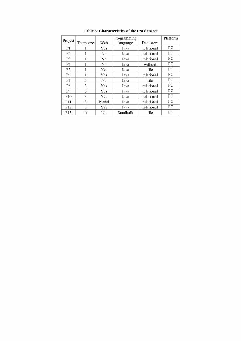
Table 3: Characteristics of the test data set

Project Team size Web Programming

language Data store Platform

P1 1 Yes Java relational PC P2 1 No Java relational PC P3 1 No Java relational PC P4 1 No Java without PC P5 1 Yes Java file PC P6 1 Yes Java relational PC P7 3 No Java file PC P8 3 Yes Java relational PC P9 3 Yes Java relational PC

P10 3 Yes Java relational PC P11 3 Partial Java relational PC P12 3 Yes Java relational PC P13 6 No Smalltalk file PC

Table 4: Project size estimates and effort

Estimated size (FP) Project Basic Comparative Final

Effort (h)

P1 96 104 110 52P2 37 35 45 42P3 185 208 157 57P4 81 61 173 54P5 37 35 35 39P6 111 121 54 44P7 155 117 163 191P8 96 69 47 163P9 155 126 136 186P10 126 100 71 171P11 177 173 72 180P12 229 234 192 204P13 148 226 278 471

Table 5: Statistical results for three estimates of all projects

Basic Comparative Final

Mean 126 123 118

Median 126 117 110

Skewness -0.01264 0.401123 0.777929

Standard deviation (σ) 56.8 68.2 72.9

Basic 0.90 0.56 Correlation

Comparative 0.69

Table 6: The errors for basic and comparative estimates

Basic Comparative Average error (FP) 46.46 42.15 Max. error (FP) 130 112 Standard deviation 40.66 35.21 Relative error (%) 39.3 35.7

Table 7: Statistical analysis for actual and calculated effort

Complete sample Partial sample

(MaxTeamSize=1)

Partial sample

(MaxTeamSize=3)

PWEactual PWEcalculated PWEactual PWEcalculated PWEactual PWEcalculated

R2 (with size) 0.450 0.457 0.916 0.981 0.914 0.982

σ 119 158 7.3 4.4 14 17

R 0.997

t-Test 0.176

Captions to illustrations Figure 1: Comparison of the size estimates Figure 2: Calculated vs. Actual effort Figure 3: Project effort as a function of size