Automated Selection of Remote Control User Interfaces in Pervasive Smart Spaces

Nirali Desai, Khomkrit Kaowthumrong, John Lebsack, Nishant Shah, Richard Han

University of Colorado at Boulder Contact: rhan@cs.colorado.edu

ABSTRACT Pervasive computing offers a vision in which every room in the home and at work will become an interactive smart space filled with wireless and wired devices whose behavior can be remotely controlled by a user, including monitors, speakers, printers, kiosks, soda machines, appliances, toys, sensors, and networked software services. The goal of this paper is to address what we term the active device resolution problem in pervasive smart spaces. Given a user with a wireless PDA or cell phone who wishes to remotely control one of N devices or services within a smart room, which of the N devices is the intended or “active” device whose user interface (UI) should be automatically selected and prefetched before the user manipulates the remote control PDA? Automated selection of the UI eases the user’s interaction with a pervasive environment, in comparison to manual selection, which is cumbersome, and directional remote control, e.g. pointing and clicking, which is insufficient to resolve the active device ambiguity when a group of devices is closely spaced, as in a home entertainment system. Our goal is to anticipate the next user interface desired by the user based on each user’s history of remote control accesses. We present a study of various prediction algorithms applied to user behavior, including first and second order Markov prediction as well as naïve Bayesian prediction, and show that the accuracy of prediction can range from 75-90%, depending upon the algorithm and the degree of training. Keywords Pervasive computing, remote control, wireless, PDA, active device resolution, service discovery, middleware, prediction, Markov, Bayes, decision tree, nearest neighbor.

1 INTRODUCTION Ubiquitous computing offers the vision of a physical environment that is fundamentally more responsive to people. Users will be able to benefit from the “smartness” of rooms and public spaces to seamlessly interact with a wide variety of internetworked wireless and wired devices, e.g. printers, monitors, speakers, wearable computers, appliances, kiosks, toys, sensors, other wireless personal digital assistants and other video-enabled mobile phones [Weiser]. Emerging technologies such as wireless pico-cell Bluetooth networks, wireless Ethernet, third generation high speed cellular systems, low power high speed microprocessors, and matchbox-sized gigabyte disks are already hastening the arrival of a world in which smart spaces are truly pervasive. A common mode of interaction with a device-filled environment is via remote control. The survey shown in Figure 1 illustrates that users already wish to extend their TV remote controls to improve their interaction with the environment, i.e. so that a single remote control can manipulate their TV as well as the lights. So-called “universal remote controls” do not have this flexibility, and tend to focus only on the home entertainment system. The X.10 protocol has been used to remotely control lights, as well as other equipment, such as window blinds, but is typically not integrated with the home entertainment system [X10]. We believe that a natural candidate for a truly universal remote control will be the PDA’s and cell phones that are already carried in the pockets of many users. Most PDA’s are already equipped with infrared, and in the future will be equipped with built-in Bluetooth and/or 802.11b wireless Ethernet. The PDA’s screen is also large enough to support a variety of UI’s to control many different devices. As the user wanders into unfamiliar smart spaces, the wireless PDA will be able to flexibly host new UI’s, unlike hardware-based “universal remote controls”. When a user with a wireless remote control PDA turns on the PDA and enters a room, the smart room discovers the PDA and allows the PDA to discover the set of registered

Figure 1. Survey from USA Today Nov. 2000 reveals the desire for multi-function remote

Figure 2. The active device resolution problem: Given N devices capable of being controlled, which user interface is the best candidate for being automatically pre-fetched into the user’s remote control, so that the user can avoid manual selection before each remote control interaction?

services that have been advertised for that environment. The discovery and advertisement of services in a smart space is enabled by a service discovery networking protocol, e.g. Sun’s Jini [Jini], Microsoft’s Universal Plug-and-Play [UPNP], Bluetooth’s service discovery [Bluetooth], the Service Location Protocol (SLP) [Guttman], and Salutation [Pascoe]. Each ubiquitous computing device is modeled as offering one or more services. In a typical smart spaces scenario, a user who walks into a room will utilize the service discovery framework to discover and control various devices: a light switch that is offering an on/off/dim lighting service; a monitor offering an output display service, and a thermostat offering a temperature control for the environment. The goal of this paper is to address what we term the active device resolution problem in pervasive smart spaces, as shown in Figure 2. Given a user with a wireless PDA or cell phone who wishes to remotely control one of N devices or services within a smart room, the task is to determine which of the N devices is the intended or “active” device whose user interface (UI) should be automatically selected and prefetched before the user manipulates the remote control PDA. When a user turns on their PDA, then our goal is to choose the best candidate UI to appear automatically on the user’s PDA given that a universal software remote control may support many UI’s. Automated selection of the UI eases the user’s interaction with a pervasive environment. Otherwise, prior to each remote control interaction, the user would have to manually select the active device by scrolling through a list of N available devices, which can be tedious. Moreover, if the devices or services are not clearly named, or if there is ambiguity when two similar devices are in the same room,

e.g. two lights, printers, or displays, then manual selection becomes even more cumbersome. Directional remote control, e.g. pointing and clicking, is insufficient to resolve the active device resolution problem when a group of devices is closely spaced, as in a home entertainment system, or when a light switch and thermostat are closely spaced together on a wall. Orientation support can help reduce N, the number of devices in a remote control’s field of vision [Priyantha2001], but does not eliminate the problem of multiple services and devices within the range of the remote control. In addition, standards such as wireless Ethernet and Bluetooth are sufficiently omnidirectional that future remote controls will be able to contact and control all services within a given radius, not just those confined to a pointing vector. A more convenient solution from the user’s perspective would be to expect the room to automatically discern the user’s intent and thereby resolve the active device to be controlled. For example, suppose the smart room understands that normally a user who has just activated the DVD player will then dim the lights. Suppose also that the light switch is located near a thermostat. Then, when the user points and clicks towards the light switch, the smart infrastructure will be able to use past behavior to predict that the user intends to communicate with the light switch rather than the thermostat. Accordingly, the appropriate user interface (UI) would automatically appear on the remote control.

2

Our goals are to understand user context, learn the remote control access patterns of each user and the system as a whole, and then determine the algorithms and policies that provide the most accurate estimate of the next user interface needed by the user. In the remainder of the paper, we explain the various prediction algorithms that we considered in Section 2, describe our experimental setup in Section 3, discuss the accuracy statistics obtained by applying the prediction algorithms in Section 4, and finish with a discussion of future and related work. 2 PREDICTION ALGORITHMS In this section, we describe each of the four prediction algorithms that we evaluated for prediction accuracy. 2.1 Nth-Order Markov Markov analysis looks at a sequence of events, and analyzes the tendency of one event to be followed by another. Using this analysis, you can generate a new sequence of random but related events, which will look similar to the original. A Markov process is useful for analyzing dependent random events - that is, events whose likelihood depends on what happened previously. It would not be a good way to model a coin flip, for example, since every time you toss the coin, there is no memory of what happened before. The sequence of heads and tails are independent events. However, many random events are affected by previous events. Our intuition was that typical user access patterns exhibit enough dependencies in behavior that a Markov-type model was worth investigating for its predictive accuracy, e.g. nearly every time after a user turns on the TV the same user then turns on the DVD. A Markov process is characterized as follows. The state ck at time k is one of a finite number in the range {1,..,M}. Under the assumption that the process runs only from time 0 to time n and that the initial and final states are known, the state sequence is then represented by a finite vector C=(c0,...,cn). Let P(ck | c0,c1 ,...,ck-1) denote the probability (chance of occurrence) of the state ck at time k conditioned on all states up to time k-1. The process is a first-order Markov if the probability of being in state ck at time k, given all states up to time k-1, depends only on the previous state, i.e. ck-1 at time k-1, i.e. P(ck | c0,c1 ,...,ck-1) = P(ck | ck-1). For an nth-order Markov process, P(ck | c0,c1 ,...,ck-1) = P(ck | ck-n ,...,ck). Figure 3 illustrates how we applied first-order Markov modeling to the access patterns of N=4 devices. Each state in the model corresponds to a device access, e.g. TV, DVD,

stereo, and alarm. The transition probabilities are constructed from the sample statistical traces we collected of user behavior, i.e. for each given state, we calculated the percentage of accesses found in the trace to the other states. For example, PTD is the sample statistic equal to the number of times the DVD was accessed after the TV. Given a current state, then a Markovian prediction algorithm would choose as the next state the one that maximizes the state transition probability from the current state. While our first order Markov model simply used the previous device accessed to predict the next device to be accessed, we also studied second and third order Markov models, e.g. what is the likelihood that the next access will be the TV given that the past two access were alarm and DVD? Since these models were constructed on a per-user

basis, then what we term as our first order Markov is technically a second-order Markov conditioned both on the user identity and the previous user action. The experimental results will be discussed in Section 4.

Figure 3. Per-user first order Markov with four states, corresponding to four remotely controlled devices. The arrows represent state transition probabilities.

2.2 Naïve Bayes Naïve Bayes classification provides a mechanism for placing a new event into the “right” category, given a set of existing categories. In our context, we are trying to predict the next event given a set of existing user accesses, i.e. given N devices, our task is to compute each of the N2 probabilities: P(A=d(k) | U=u0, PA=d(j)), for k and j=1..N,

3

where A=access, d(k) is device k, U=user for a fixed user 0, and PA=previous access. Given these probabilities, then Naïve Bayes chooses the next device which maximizes the transition probability from the previously accessed device. The Bayes relation can be stated as P(A B) = P(A|B)P(B), so that P(A B C) = P(A)P(B|A)P(C|A. B). The naïve Bayes classifier uses the following approach: max P(A(i)|B) = max P(B|A(i))*P(A(i)) / P(B) = max P(B|A(i))*P(A(i)), maximizing over i. Therefore, we choose the k’th device that maximizes the following expression: max P(A=d(k) | U=u0, PA=d(j)), = max P(A=d(k))*P(U=u0|A=d(k))*P(PA=d(j)|A=d(k)) (1) Each of the elements in Equation 1 can be estimated from our trace data. For example, if d(k)=DVD, the user u0 is John, and d(j)=TV, then equation 1 becomes a maximization of the following probabilistic expression whose elements can be estimated from our data, namely: P(A=DVD)*P(U=John|A=DVD)*P(PA=TV|A=DVD). 2.3 Nearest Neighbor Among the different paradigms of learning in Artificial Intelligence, there is one class of models, which uses observed patterns in data to create classification rules, and another class of models, which does not depend on these inferring rules and works directly from the stored data available. In this section we concentrate on the latter class of models known as Memory-Based Reasoning models. [Stanfill86] One memory-based reasoning algorithm is the Nearest Neighbor Algorithm. Nearest Neighbor suited our prediction problem because the likelihood of finding an identical match in a table or memory is small, so it would be more convenient to find the most similar case to our present situation using some distance metric over the stored cases. A solution using this method would involve three components: the set of stored cases, the distance metric used to compute the distance to similar cases and the number of nearest neighbors to retrieve, say k. In our context, we have to predict the appropriate user interface based on what day of the week it is, what time of the day it is, and what were the previous actions performed by the user. The current versions of the above attributes are used to retrieve k number of similar cases from the stored cases.

Once these k neighbors are retrieved their attributes are examined and an absolute distance is computed for the new case from each of these cases. The prediction could then be based on the outcome of the case that is nearest to the current case. One important point to note is that not all attributes of the data set would contribute to this distance function. Some of them can be irrelevant and can decrease the accuracy of prediction. Thus the success of this method would depend on parameters like determining the optimum set of attributes and the optimum value of neighborhood size N. The effectiveness of a distance-based solution is greatly enhanced by specialized hardware or by presorting the data for comparisons [Polyanalyst] [Weiss98]. 2.4 Decision Tree Another algorithm used for the prediction analysis was the decision tree algorithm. Unlike the Nearest Neighbor

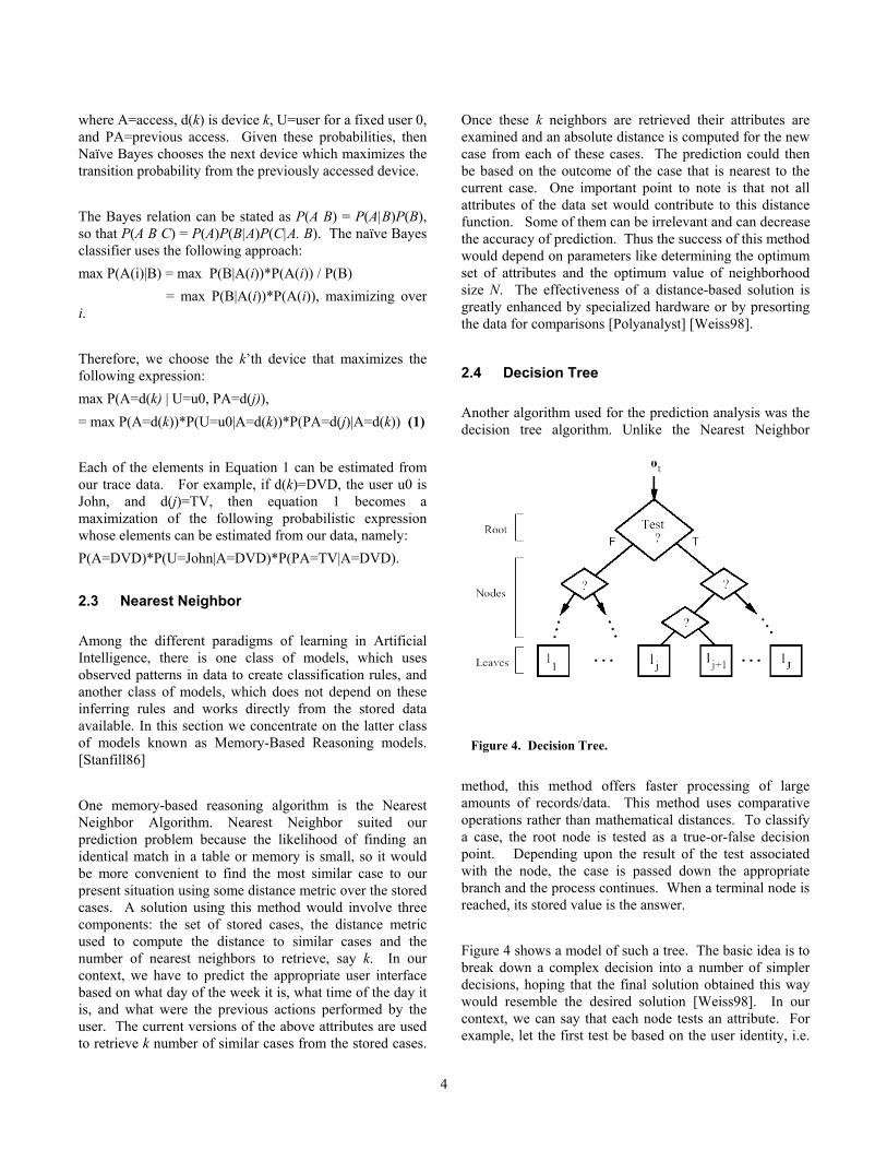
method, this method offers faster processing of large amounts of records/data. This method uses comparative operations rather than mathematical distances. To classify a case, the root node is tested as a true-or-false decision point. Depending upon the result of the test associated with the node, the case is passed down the appropriate branch and the process continues. When a terminal node is reached, its stored value is the answer.

Figure 4. Decision Tree.

Figure 4 shows a model of such a tree. The basic idea is to break down a complex decision into a number of simpler decisions, hoping that the final solution obtained this way would resemble the desired solution [Weiss98]. In our context, we can say that each node tests an attribute. For example, let the first test be based on the user identity, i.e.

4

is this user X? If yes, then is the most recent access a TV? If yes, then is the current time in the evening? If yes, then predict that the next access will be DVD. If no, then predict that the next access will be the stereo. The decision tree would take a different branch based on the conditions of each access. Various decision trees could be generated based on which node is selected as the root and the best among those could be selected for the prediction.

3 EXPERIMENTAL SETUP Traces were collected over the course of three weeks in the home of one of the co-authors. Three unique users manually recorded their usage of four devices: a TV, a stereo, a DVD player, and a burglar alarm. The devices were all within the same room. The users recorded the following information on the log: day of the week, time of day, device being controlled, and the action (on/off). The logs also showed the identity of each user. In the future we plan to collect more samples from more users using more devices, e.g. lights. We also plan to explore the use of automated collection of data instead of manual logs. The traces included a total of 138 samples. For the experiments, these samples were divided into training sets and test sets. These divisions were done in two different ways. The first method consisted of:

• Selection of 34 examples (25% of the total) chosen at random, forming the test data.

• Selection of training sets ranging in size from 1 to 100 samples, chosen at random from the total sample.

The second method involved partitioning the samples into separate training and test sets according to the sequence in which they were logged. The first 100 samples were used as training sets, in sizes ranging from 10 to 100 in increments of 10. These training sets were also assembled according to the sequence in which they were logged, i.e. the first 10 samples in the log were used for the training set of size 10, the first 20 samples in the log were used for the training set of size 20, etc. For this second method, the remaining 38 samples in the log were set aside as the test data The performance of the algorithms was evaluated using a combination of commercial machine-learning tools and applications written specifically for this project. The commercial tool was PolyAnalyst from Megaputer

Intelligence Inc [Polyanalyst].1 This program conveniently includes ten different machine-learning algorithms, of which two were suitable for our problem: nearest neighbor and decision tree. 2 These are well suited for our predictive classification problem, i.e. the goal of the prediction is not to produce a number, but a classification: the particular device the user wishes to use. The prediction accuracy of the nearest neighbor and decision tree algorithms were all measured using PolyAnalyst and the first mixed method of selecting training and test sets described above. These results are shown on Figure 7 and will be discussed in the next section. The prediction accuracy of the Markov and Naïve Bayes algorithms relied on software implementations written by two of the co-authors specifically for these experiments. Figure 6 illustrates the accuracy of these algorithms using only the second partitioned method of creating training and test sets, while Figure 7 illustrates the accuracy using only the first mixed method. These results are explained in the next section.

4 EXPERIMENTAL RESULTS Our initial findings suggest that prediction is feasible, and can achieve an accuracy of 75-90% depending on the length of the training set and the algorithm used. However, before we begin with the analysis of any of the algorithms presented in this paper, we need a baseline for comparison. Figure 5 depicts the distribution of device accesses in the first and second test sets. The most common device chosen in all the training sets was the TV. Hence, a useful baseline algorithm to compare against would be a most-common device (MCD) algorithm that chose the device with the largest percentage of the distribution. In our study, an MCD algorithm that picked the TV for every test sample would be right 58 percent of the time for the first set of training and test data, and 53 percent for the second method. Hence, any of our the other prediction

1 This commercial product was used on a trial basis for these tests.

Other tools implementing the same algorithms (nearest neighbor and decision tree) are available without charge for academic use.

2 The other algorithms are not suitable for this test domain. Some are unsuitable because they require numerical target attributes. The target attribute in this test was a classification among several strings. Other algorithms were unsuitable because they solve clustering problems.

5

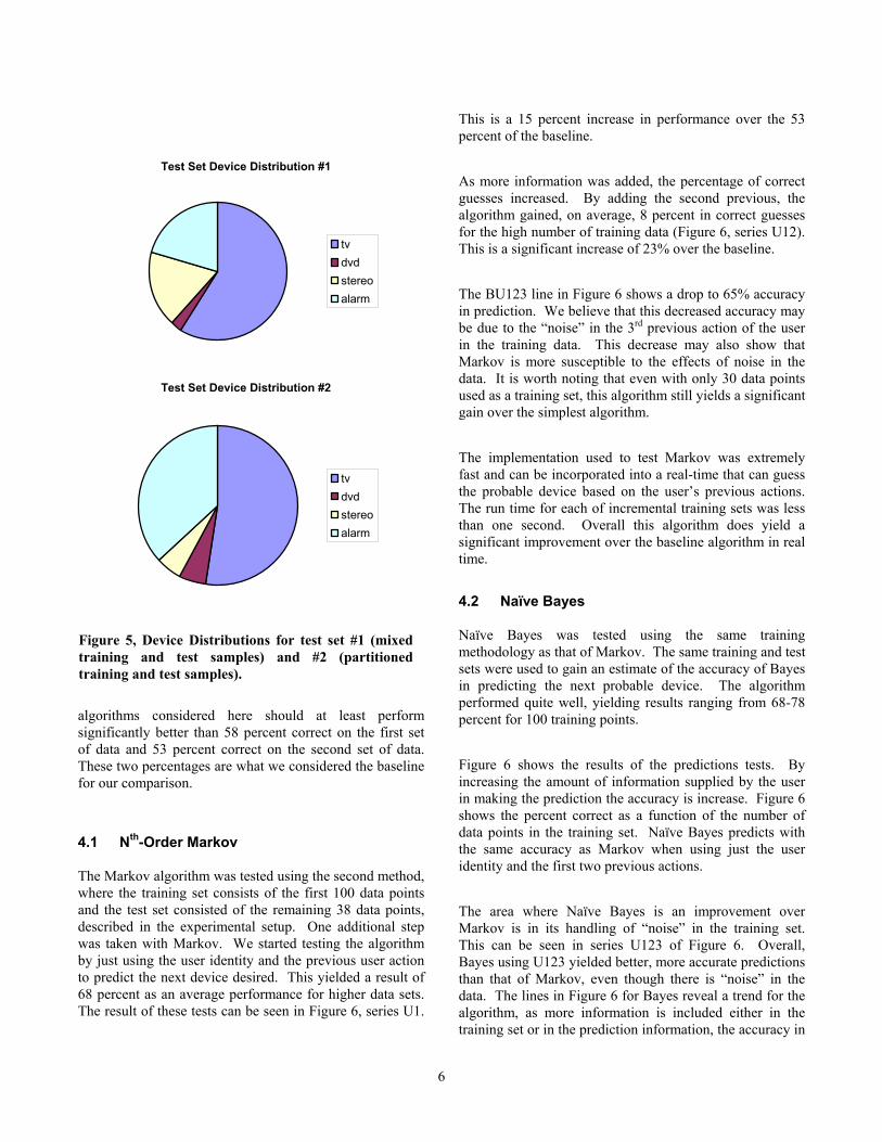
algorithms considered here should at least perform significantly better than 58 percent correct on the first set of data and 53 percent correct on the second set of data. These two percentages are what we considered the baseline for our comparison. 4.1 Nth-Order Markov The Markov algorithm was tested using the second method, where the training set consists of the first 100 data points and the test set consisted of the remaining 38 data points, described in the experimental setup. One additional step was taken with Markov. We started testing the algorithm by just using the user identity and the previous user action to predict the next device desired. This yielded a result of 68 percent as an average performance for higher data sets. The result of these tests can be seen in Figure 6, series U1.

This is a 15 percent increase in performance over the 53 percent of the baseline.

Test Set Device Distribution #1

tvdvdstereoalarm

Test Set Device Distribution #2

tvdvdstereoalarm

Figure 5, Device Distributions for test set #1 (mixed training and test samples) and #2 (partitioned training and test samples).

As more information was added, the percentage of correct guesses increased. By adding the second previous, the algorithm gained, on average, 8 percent in correct guesses for the high number of training data (Figure 6, series U12). This is a significant increase of 23% over the baseline. The BU123 line in Figure 6 shows a drop to 65% accuracy in prediction. We believe that this decreased accuracy may be due to the “noise” in the 3rd previous action of the user in the training data. This decrease may also show that Markov is more susceptible to the effects of noise in the data. It is worth noting that even with only 30 data points used as a training set, this algorithm still yields a significant gain over the simplest algorithm. The implementation used to test Markov was extremely fast and can be incorporated into a real-time that can guess the probable device based on the user’s previous actions. The run time for each of incremental training sets was less than one second. Overall this algorithm does yield a significant improvement over the baseline algorithm in real time. 4.2 Naïve Bayes Naïve Bayes was tested using the same training methodology as that of Markov. The same training and test sets were used to gain an estimate of the accuracy of Bayes in predicting the next probable device. The algorithm performed quite well, yielding results ranging from 68-78 percent for 100 training points. Figure 6 shows the results of the predictions tests. By increasing the amount of information supplied by the user in making the prediction the accuracy is increase. Figure 6 shows the percent correct as a function of the number of data points in the training set. Naïve Bayes predicts with the same accuracy as Markov when using just the user identity and the first two previous actions. The area where Naïve Bayes is an improvement over Markov is in its handling of “noise” in the training set. This can be seen in series U123 of Figure 6. Overall, Bayes using U123 yielded better, more accurate predictions than that of Markov, even though there is “noise” in the data. The lines in Figure 6 for Bayes reveal a trend for the algorithm, as more information is included either in the training set or in the prediction information, the accuracy in

6

predicting the next device is increased. Overall naïve Bayes has yielded the best gain from the simplest algorithm so far, with a best performance of 78 percent correct at 100 data points in the training set. This fact, when coupled with a very fast run-time (less than one second), makes Naïve Bayes a very prime candidate for implementation in a real-time system. 4.3 Nearest Neighbor The nearest neighbor algorithm showed promising results. All training and test sets for were assembled using the first method described in section 3. On six of the larger training sets, this algorithm was able to make predictions with 94 percent accuracy. For example, on a randomly-picked training set of 66 samples, nearest neighbors made the predictions shown on Table 1.

Real/Pred

TV Alarm Stereo DVD

TV 20 0 0 0 Alarm 0 7 0 0 Stereo 2 0 4 0 DVD 0 0 0 1

Table 1. Nearest neighbor predictions based on randomly selected training set of size 66, tested on random sample of 25 percent of all data. Entries on the diagonal in Table 1 show correct predictions. All others show errors. Here, the algorithm made just two errors out of 34, twice predicting that the user wanted the TV interface when the user actually chose the stereo. Another example of the performance of nearest neighbor is shown in Table 2. This also shows two mistakes out of 34, the first a prediction of TV when the user actually picked DVD and the second a prediction of TV when the user wanted the alarm. Real/Pred TV Alarm Stereo DVD TV 20 0 0 0 Alarm 1 6 0 0 Stereo 0 0 6 0 DVD 1 0 0 0 Table 2. Nearest neighbor predictions based on randomly selected training set of size 90, tested on random sample of 25 percent of all data.

The overall performance of nearest neighbor is shown on Figure 7. The x-axis is the size of the training set. The y-axis is the percentage of correct predictions out of the test set of 34 examples (assembled using the first method described in Section 3). No results are shown for training sets of fewer than 10 examples because this implementation of the algorithm requires a training set of at least 10. Some data points are missing because of this implementation’s inability to apply the rule based on certain training sets against the random sample. The authors believe this inability reflects an idiosyncrasy of the implementation. The results show that nearest neighbor needs a training set of between 20 and 30 examples before it produces meaningful predictions. But once the algorithm can train on at least 80 examples, it makes accurate predictions about 90 percent of the time. It is important to note that a prediction accuracy of 58 percent on this chart represents the accuracy of the simplest classification rule, the MCD algorithm described above. This algorithm requires no computation other than counting which classification occurs most frequently in the data, here the TV. The MCD algorithm would have 58 percent accuracy on this test set with no learning at all. This percentage shows up again in the decision tree results discussed in the next section. The variation in the accuracy of the nearest neighbor algorithm shown on Figure 7 is the result of the two factors: noise in the data and the random selection process for the training sets. Noise in this data means the user doesn’t always follow a consistent pattern. The random selection process for the training sets means that sometimes the training set will contain relatively few of the examples which show a pattern and relatively many of the examples which do not follow a pattern. Even if a particular user is usually consistent, random selection means that the consistent examples will sometimes be underrepresented in the training set. A significant issue with the nearest neighbor algorithm is run time. In these experiments, the run time was about 1 second for each 10 items in the training set, i.e., a 10 second run time for a training set of 100. Obviously this delay would not be acceptable to the user. The solution is to run the algorithm off line. After the off line analysis produces a classification rule, that rule could be quickly applied to a new example. Moreover, once there are sufficient examples of the system and the users’ behavior, it would be feasible to run the algorithm on the full training set only at intervals, with the length of the intervals determined adaptively. The system could be implemented to adapt the interval based on how much difference there is

7

between the former and current rules. If the full analysis produces basically the same rule, the interval could be lengthened. If the rule changes beyond some threshold, the interval to the next full analysis could be reduced. 4.4 Decision Tree The decision tree algorithm demonstrated that it could induce classification rules from the data, but not as well as the nearest neighbor algorithm. The accuracy of decision tree was generally 20 percent worse than nearest neighbor. All training and test sets were assembled using the first method described in section 3. The decision tree algorithm also required a larger training size before it could produce meaningful results. Until the decision tree could train on at least 45 examples, it made predictions only with the accuracy of the simplest classification rule, 58.82 percent. Whenever the decision tree algorithm trained on sets of fewer than 45 examples, its prediction rule was just to predict the TV every time. Figure 7 also shows the results of the naïve Bayes and Markov algorithms on the same training and test sets used in the analysis of decision tree and nearest neighbor. The results for naïve Bayes and Markov are shown for training sets of sizes in increments of 10; lines do not connect those points. Run time is also an issue for the decision tree algorithm. Although not as slow as nearest neighbor, this

implementation of decision tree still ran too slowly to allow on line use of the algorithm. The off line approach discussed above would also be required for decision tree.

4.5 Future work The preliminary findings of this research suggest many areas for improvement. We plan to extend our analysis to collect longer traces of user behavior then have been shown here. Such traces should be collected in an automatic fashion, incorporating many more users over longer time scales, and should include more devices such as light switches, remotely controllable phones, etc. Longer traces will help us provide clearer validation of our Markovian assumptions. Also, accuracy is not the only metric. We would also like to compare the speed of prediction of various algorithms. Some algorithms are considerably more compute-intensive than others, which will affect their real-time performance. For non-real-time algorithms, learning can be performed off-line to isolate the user from the latency of prediction. We would like to provide more precise measures of the complexity of each algorithm, in order to measure how close to real time each algorithm could come, given that the state space of N devices or parameters may be much larger, especially of k-th order Markov modeling.

8

9

Markov Prediction Accuracy vs. Training Set Size

0.00%

10.00%

20.00%

30.00%

40.00%

50.00%

60.00%

70.00%

80.00%

90.00%

100.00%

0 10 20 30 40 50 60 70 80 90 100

Training Set Size

Perc

ent C

orre

ct

U1U12U123

Naive Bayes Prediction Accuracy vs. Training Set Size

0.00%

10.00%

20.00%

30.00%

40.00%

50.00%

60.00%

70.00%

80.00%

90.00%

100.00%

0 10 20 30 40 50 60 70 80 90 100

Training Set Size

Perc

ent C

orre

ct

U1U12U123

Figure 6. Markov and Naive Bayes prediction accuracies based on the second method of partitioned training and test samples

5 RELATED WORK Prior work on remote control of applications via a PDA has focused on controlling a video conferencing application [Hodes99a] as well as providing an XML framework for controlling lights and stereo components [Hodes99b]. These efforts focus on manual control and selection, and do not address automated selection and prediction. In CMU’s Pebbles project, a PDA is used to control a single PC’s screen and various PC applications, including PowerPoint as well as a Web browser [Myers98, Myers2000]. Cellular phones have been used as remote controls to purchase sodas from vending machines in Nordic countries using the Jalda payment standard developed [Jalda]. So-called “universal remote controls” represent inflexible hardware solutions that only interact with the components in a home entertainment system. The challenges introduced by more general ubiquitous computing environments populated with N devices are only beginning to be addressed [Hodes99b, Han2000]. Multi-device ubiquitous computing is largely a new topic, as few researchers have yet considered the implications of supporting multiple devices simultaneously in the context of remote control applications. Stanford’s multibrowsing project [Johnson2001] investigates user interaction with multiple output displays. Web pages can be moved between multiple smart displays using a middleware infrastructure in conjunction with Web browser plugins. Similarly, multi-device user interfaces have been proposed in which a user can “pick” an object from a PDA and “drop” it on a PC screen or digital whiteboard using middleware [Rekimoto98]. Other work has focused on partitioning of a dual-device user interface between a wireless PDA remote control and a single other device, namely an interactive TV [Robertson96]. These efforts are primarily concerned with moving data between devices and do not address the problem of active device resolution given multiple controllable devices in a remote control’s field of vision. Also, these efforts are largely specialized outside of standard service discovery frameworks. As mentioned in Section 1, a key component of the developing infrastructure for ubiquitous computing is based on the discovery and advertisement of services. Local-area service discovery protocols include Jini, UPNP, Bluetooth’s service discovery, SLP, and Salutation. Both Jini and UPNP use IP multicast on well-known addresses to advertise and discover services. Jini and SLP both employ a centralized directory or registry, i.e. devices advertise their presence by registering themselves with the directory. UPNP uses a decentralized peer-only method in which devices multicast directly to other devices. Jini is built entirely on top of Java except for an initial bootstrap

discovery protocol, and downloads Java objects and service descriptions over Java’s Remote Method Invocation (RMI) to Java Virtual Machines (JVM) on all devices (those ubiquitous computing devices too limited to support a JVM can still participate by using a JVM proxy). UPNP assumes IP packet delivery and utilizes HTTP as a transport mechanism for XML service descriptions. Bluetooth’s service discovery protocol SDP is lower layer and network-specific. Depending upon the service discovery protocol in use, there are implications on the user interface’s flexibility. Jini imposes a UI upon the user defined by the service provider, since the Jini client downloads a vendor-defined Java executable object that implements the provider’s UI. UPNP provides more freedom for the client side to implement its own UI, since UPNP simply exposes the control variables available at a service provider for the client to adjust. UPNP thereby allows the client to decide which control variables to adjust and how to convey these controllable variables via a UI. This paper has not focused on the look-and-feel of the UI on the handheld, nor on how this look-and-feel may be constrained by service discovery, but instead focuses on which of N UI’s should be automatically presented to the user. Early work on intelligent environments includes a study of predicting a user’s movement within a smart home using neural networks [Mozer98]. This study focused on triggering lighting based on the user’s location and past pattern of behavior in turning on and off lights. Our study extends this work to focus on predicting more general kinds of user activity. Georgia Tech has built an “Aware Home” to assist those who may be impaired with Alzheimer’s [Fox2001]. Microsoft’s EasyLiving project has created an intelligent living room implements a follow-me application that tracks user motion using stereo cameras in order to keep a user interface in front of a user for easy access [EasyLiving]. 6 SUMMARY In this paper, we addressed the active device resolution problem of predicting the user interface desired by a user of a remote control when there are N devices in the vicinity that can be controlled. We collected real world traces of user behavior and applied several predictive algorithms, including Markov, naïve Bayes, nearest neighbor, and decision tree algorithms. Our initial findings suggest that prediction is feasible, and can achieve an accuracy of 75-90% depending on the length of the training set and the algorithm used. Nearest neighbor achieved the highest accuracy of 90%, but operates too slowly for real time prediction. The naïve Bayes classifier achieved a

10

Prediction Accuracy-All Algorithms

0

10

20

30

40

50

60

70

80

90

100

0 20 40 60 80 100

Training Set Size

Perc

ent C

orre

ct

NN DT NBM

Figure 7. Prediction accuracy of Nearest Neighbor (NN), Decision Tree (DT), Naïve Bayes (NB), and Markov (M) using the first method for assembling the training and test sets. Test set size 34, randomly selected.

prediction accuracy of 78% after 100 training samples while peering back 3 user access events, and is capable of near real time operation.

7 Acknowledgements We’d like to thank Olivier Verscheure of IBM’s Thomas J. Watson Research Center for some early discussions on active device resolution. Thanks also to Ben Lebsack and Holly Bennett for their assistance in collecting traces. 8 REFERENCES [Bluetooth] Bluetooth Service Discovery, http://www.bluetooth.com. [EasyLiving] B. Brumitt, B. Meyers, J. Krumm, A. Kern, S. Shafer, "EasyLiving: Technologies For Intelligent Environments," Handheld and Ubiquitous Computing, September 2000. www.research.microsoft.com/easyliving. [Fox2001] C. Fox, “Genarians: the Pioneers of Pervasive Computing Aren’t Getting Any Younger,” Wired, November. 2001, pp. 187-193.

[Guttman] E. Guttman, C. Perkins, J. Veizades, and M. Day. Service location protocol, version 2. Request for Comments 2608, Internet Engineering Task Force, June 1999. [Han2000b] R. Han, V. Perret, M. Naghshineh, “WebSplitter: A Unified XML Framework For Multi-Device Collaborative Web Browsing”, ACM Conference on Computer Supported Cooperative Work (CSCW), Dec. 2000, pp. 221-230. [Hodes99a] T. Hodes, R.Katz, “A Document-based Framework for Internet Application Control,” 2nd USENIX Symposium on Internet Technologies and Systems (USITS), 1999, pp. 59-70. [Hodes99b] T. Hodes, M. Newman, S. McCanne, R. Katz, J. Landay, “Shared Remote Control of a Video Conferencing Application: Motivation, Design, and Implementation,” SPIE Multimedia Computing and Networking (MMCN), Proc. SPIE, vol. 3654, 1998 (conf. held Jan 1999), pp. 17-28. [Jalda] Jalda Payment Standard for the Fixed and Mobile Internet, http://jalda.com. [Jini] Sun’s Jini architecture, http://www.jini.org

11

[Johnson2000] B. Johanson, S. R. Ponnekanti, C. Sengupta, A.Fox., Technical Note in UBICOMP 2001, Sept. 2001. [Mozer98] M. Mozer, “The Neural Network House: An Environment that Adapts to its Inhabitants”, Intelligent Environments, Papers from the AAAI Spring Symposium, March 23-25, 1998, Technical Report SS-98-02, AAAI Press. [Myers98] B. Myers, H. Stiel, and R. Gargiulo. "Collaboration Using Multiple PDAs Connected to a PC." Proceedings CSCW'98: ACM Conference on Computer-Supported Cooperative Work, November 14-18, 1998, Seattle, WA. pp. 285-294. See also http://www.cs.cmu.edu/~pebbles/ [Myers2000] B. Myers, “Using Multiple Devices Simultaneously for Display and Control,” IEEE Personal Communications Magazine, October 2000, pp. 62-65. [Pascoe] R. Pascoe, “Building Networks on the Fly,” IEEE Spectrum, March 2001, pp. 61-65.

[Polyanalyst] Polyanalyst commercial software implementing nearest neighbor algorithm, www.megaputer.com.

[Priyantha2001] N. Priyantha, A. Miu, H. Balakrishnan, S. Teller, “The Cricket Compass for Context-Aware Applications”, ACM MobiCom, 2001. [Rekimoto98] J. Rekimoto, “A Multiple Device Approach for Supporting Whiteboard-based Interactions,” Human Factors in Computing Systems (CHI) 1998, pp.344-351. [Robertson96] S. Roobertson, C. Wharton, C. Ashworth, M. Franzke, “Dual Device User Interface Design: PDA’s and Interactive Television,” SIG CHI 1996, pp. 79-86. [Stanfill86] C. Stanfill, and D. Waltz, "Toward Memory-Based Reasoning," Communications of the ACM 29(12), 1986, , pp. 1213-1228. [UPNP] Universal Plug and Play Service Discovery, http://www.upnp.org/ [X10] X10 Remote Control, http://www.x10.com [Weiser] M. Weiser, "Some Computer Science Problems in Ubiquitous Computing," Communications of the ACM, July 1993, pp. 75-83. (reprinted as "Ubiquitous Computing". Nikkei Electronics; December 6, 1993; pp. 137-143.) [Weiss98] S. Weiss, N. Indurkhya, “Predictive Data Mining – a practical guide”, Morgan Kaufmann Publishers,Inc, 1998.

12