Consist

ent *Complete *

Well D

ocumented*Easyt

oR

euse* *

Evaluated

*CAV*Ar

tifact *

AEC

Automated Resource Analysiswith Coq Proof Objects‹

Q. Carbonneaux1, J. Hoffmann2, T. Reps3, and Z. Shao1

1 Yale University2 Carnegie Mellon University

3 University of Wisconsin and GrammaTech, Inc.

Abstract. This paper addresses the problem of automatically performingresource-bound analysis, which can help programmers understand theperformance characteristics of their programs. We introduce a method forresource-bound inference that (i) is compositional, (ii) produces machine-checkable certificates of the resource bounds obtained, and (iii) features asound mechanism for user interaction if the inference fails. The techniquehandles recursive procedures and has the ability to exploit any knownprogram invariants. An experimental evaluation with an implementationin the tool Pastis shows that the new analysis is competitive with state-of-the-art resource-bound tools while also creating Coq certificates.

1 IntroductionTo help developers better understand the performance of programs at compiletime, the programming-language research community has been developing tech-niques and tools that can automatically and statically analyze the resourceconsumption of programs [1, 2, 4, 7, 13, 20, 23, 28, 31]. Most of these techniquesderive symbolic worst-case bounds that depend on the sizes of program variablesor the arguments of a function. Deriving such bounds for arbitrary programsis an undecidable problem. However, existing tools deliver impressive resultsfor certain classes of programs. Tools deriving bounds on imperative programsinclude KoAT [10], Rank [5], CoFloCo [16], Loopus [30], and C4B [11]. RAML [17]is able to derive complex bounds on functional programs.

State-of-the-art bound analysis tools suffer from two major shortcomings.First, when the inference of a resource bounds fails, the user has no other choicethan to either rewrite the input program or modify the tool itself (the second

‹ Supported, in part, by a gift from Rajiv and Ritu Batra; by NSF under grants1521523 and 1319671; by AFRL under DARPA MUSE award FA8750-14-2-0270,DARPA STAC award FA8750-15-C-0082, and DARPA award FA8750-16-2-0274;and by the UW-Madison Office of the Vice Chancellor for Research and GraduateEducation with funding from the Wisconsin Alumni Research Foundation. The U.S.Government is authorized to reproduce and distribute reprints for Governmentalpurposes notwithstanding any copyright notation thereon. Any opinions, findings,and conclusions or recommendations expressed in this publication are those of theauthors, and do not necessarily reflect the views of the sponsoring agencies.

option being only available to experts). Second, many automated tools are basedon sophisticated algorithms relying on subtle invariants for their correctness.Even tools based on time-tested programming-language devices like type systemsand program logics have complex implementations that are prone to bugs.

The goal of this paper is to address these shortcomings. We base our workon automatic amortized resource analysis (AARA), a technique that staticallyderives concrete (non-asymptotic) resource bounds. AARA is implemented inthe tools C4B for imperative programs and RAML for functional programs. Thebenefits of AARA include compositionality—by generating compositional andlocal constraint systems—and reduction of resource-bound inference to efficientoff-the-shelf linear programming (LP).

Contributions. First, we present a new unifying framework for proving thesoundness of AARA-based systems for low-level code. The framework appliesdirectly to low-level programs parameterized with abstract base constructs. Thisparameterized presentation allows, similarly to the theory of abstract interpreta-tion, multiple instantiations depending on the programs to be analyzed. We alsointroduce rewrite functions, a new technical device to encode weakening that isamenable to sound user interaction.

Second, to demonstrate the effectiveness of these new ideas, we have imple-mented them in a new tool called Pastis.– Thanks to our new parametric framework, Pastis is the first AARA-based tool

to generate polynomial bounds on low-level integer programs with recursiveprocedures.

– Thanks to rewrite functions, Pastis is the first resource analysis tool to providea sound mechanism for user interaction when the inference of a bound fails.

– Thanks to the logical foundations of our framework, and to the certificatesprovided by the LP solver, Pastis is the first resource analysis tool able toautomatically generate proof certificates of the validity of its bounds.Third, to show that Pastis is practical, we have implemented an LLVM

frontend to our new analysis and evaluated it on more than 200,000 lines ofC code against state-of-the-art tools. Surprisingly for a tool generating proofobjects, we are able to report that Pastis is competitive and can successfullygenerate many polynomial bounds.

Acknowledgments. We thank Vilhelm Sjöberg and Lionel Rieg for their helpfulsuggestions during the implementation of proof certificates in Coq.

2 SettingPrograms will be represented as standard interprocedural control-flow graphs.This assumption does not tie the presentation of our analysis to a specific set ofstatements; moreover, it allows the technique to be applied to unstructured inputprograms, including ones written in bytecode and other low-level languages.

Syntax. A program is represented as a directed graph where nodes are programpoints and edges bear program actions. Intuitively the program counter jumpsfrom node to node following edges and updates the program state according to

2

p`, v Ð e, `1q P E

p`, σq Ñ p`1, σrJeKσ{vsqp`,weaken, `1q P E

p`, σq Ñ p`1, σq

p`, guard e, `1q P E JeKσ P OK

p`, σq Ñ p`1, σq

p`, call P, `1q P E

∆pP q “ p_, `e, `xqp`e, σq Ñ˚ p`x, σ1q

σ2pvq “

"

σ1pvq if v P Gσpvq otherwise

p`, σq Ñ p`1, σ2q

Fig. 1. Mixed-step semantics of a program pE,∆,Gq. Non-call steps use a classicsmall-step transition while calls are atomically executed using Ñ˚.

the actions it encounters. We use the three sets L, V , and P , respectively, for theprogram points, the variable names, and the procedure names.

A procedure is represented by a tuple pL, `e, `xq where L Ď V is the set oflocal variables for the procedure and `e, `x P L are respectively the entry andexit points of the procedure.

Act :“ v Ð e | call P | guard e | weaken

An action can be the assignment of a variable v Ð e where v P V and e is anexpression. We leave the syntax of expressions abstract because it is irrelevantfor most of the presentation that follows. An action can also be a call call P toa procedure P P P. The arguments and return values are passed using globalvariables. We also include guards as actions. They are used to represent conditionalstatements and block the execution if their condition is not validated at runtime.Finally, an action can be an explicit weakening hint weaken. Such a hint canbe inserted by the user or by a pre-processing heuristic; it does not have anysemantic effect but is used by our analysis to perform potential rewrites.

We now define a program as a triple pE,∆,Gq where:– E Ď pLˆActˆ Lq is the set of all edges in the program;– ∆ is a map from procedure names P to procedures;– and G Ď V is the set of global variables.In addition, we require that no two procedures in the program share any localvariables, and that the sets of global variables and local variables are disjoint.These properties can be ensured by pre-processing.Semantics. An execution state is a pair p`, σq where σ P Σ is a program statethat maps variables V to a value domain D, and ` P L is the program counter.

We define single-step execution of the program as a transition relation onexecution states. When evaluating an edge of the program, the change madeto the program state is determined by the action labelling the edge. For eachprogram state σ we assume that we have an evaluation function J¨Kσ that mapsexpressions to the value domain D. We also require the presence of a predicateOK Ď D on the value domain to check the validity of conditions in guards (e.g.,a singleton ttrueu). We use σru{vs to denote a new program state that extends σby updating the binding of v to the value u. The complete operational semanticsof programs is given in Figure 1. We write Ñ˚ to denote the reflexive transitiveclosure of the step relation Ñ.

3

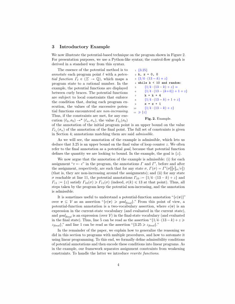
3 Introductory Example

We now illustrate the potential-based technique on the program shown in Figure 2.For presentation purposes, we use a Python-like syntax; the control-flow graph isderived in a standard way from this syntax.

1 t3.25u2 k, z = 0, 03 t1{4 ¨ p13´ kq ` zu4 while k < 10 and random:5 t1{4 ¨ p13´ kq ` zu “6 t1{4 ¨ p13´ pk`4qq ` 1` zu7 k = k + 48 t1{4 ¨ p13´ kq ` 1` zu9 z = z + 1

10 t1{4 ¨ p13´ kq ` zu11 ě tzu

Fig. 2. Example.

The essence of the potential method is toannotate each program point ` with a poten-tial function Γ` P pΣ Ñ Qq, which maps aprogram state to a rational number. In theexample, the potential functions are displayedbetween curly braces. The potential functionsare subject to local constraints that enforcethe condition that, during each program ex-ecution, the values of the successive poten-tial functions encountered are non-increasing.Thus, if the constraints are met, for any exe-cution p`0, σ0q Ñ˚ p`n, σnq, the value Γ`0pσ0qof the annotation of the initial program point is an upper bound on the valueΓ`npσnq of the annotation of the final point. The full set of constraints is givenin Section 4; annotations matching them are said admissible.

As we will see, the annotation of the example is admissible, which lets usdeduce that 3.25 is an upper bound on the final value of loop counter z. We oftenrefer to the final annotation as a potential goal, because that potential functiondefines the quantity we are looking to bound. In the example, the goal is tzu.

We now argue that the annotation of the example is admissible: (i) for eachassignment “v Ð e” in the program, the annotations Γ and Γ 1, before and afterthe assignment, respectively, are such that for any state σ, Γ pσq “ Γ 1pσrJeKσ{vsq(that is, they are non-increasing around the assignments); and (ii) for any stateσ reachable at line 11, the potential annotations Γ10 :“ t1{4 ¨ p13´ kq ` zu andΓ11 :“ tzu satisfy Γ10pσq ě Γ11pσq (indeed, σpkq ď 13 at that point). Thus, allsteps taken by the program keep the potential non-increasing, and the annotationis admissible.

It is sometimes useful to understand a potential-function annotation “tepvqu”over v Ď V as an assertion “tepvq ě goalfinalu.” From this point of view, apotential-function annotation is a two-vocabulary assertion, where epvq is anexpression in the current-state vocabulary (and evaluated in the current state),and goalfinal is an expression (over V) in the final-state vocabulary (and evaluatedin the final state). Thus, line 5 can be read as the assertion “t1{4 ¨ p13´ kq ` z ězfinalu,” and line 1 can be read as the assertion “t3.25 ě zfinalu.”

In the remainder of the paper, we explain how to generalize the reasoning wedid in this section to programs with multiple procedures, and how to automate itusing linear programming. To this end, we formally define admissibility conditionsof potential annotations and then encode these conditions into linear programs. Asin the example, our framework separates assignment constraints from weakeningconstraints. To handle the latter we introduce rewrite functions.

4

4 Interprocedural Potential AnnotationsIn this section, we consider a fixed program pE,∆,Gq. A procedure P in theprogram has entry and exit points Pe, Px P L, respectively. A state σ at ` P L isreachable from pPe, σ0q when there is an execution trace

pPe, σ0q Ñ p`1, σ1q . . .Ñ p`n, σnq,

such that σn “ σ ^ `n “ `, or p`n, call Q,_q P E and σ at ` is reachable frompQe, σnq. The latter disjunct is necessary because we use mixed-step semantics:calls are represented by a single step Ñ, and Ñ˚ always relates two points in thesame procedure. Finally, we say that σ at ` is reachable (from Pe), when there isan initial state σ0 such that σ at ` is reachable from pPe, σ0q.

A potential function is a function that maps program states to rationalnumbers. A procedure annotation Γ associates a potential function Γ` with eachprogram point ` in a procedure. An interprocedural potential annotation (IPA) Ψmaps each procedure name P to a set of procedure annotations ΨpP q. Sets ofannotations are used because, depending on the context in which a procedureis called, different annotations might be used. A goal is a potential function ofspecial interest: it is the quantity at the end of the program that we are seekingto bound in terms of the initial state.

Definition 1 (Admissible IPA). We say that an IPA Ψ for the programpE,∆,Gq is admissible for a goal g and an entry and exit point Se and Sx ina procedure S when:

(A1) DΓ P ΨpSq. ΓSx “ g;and for every procedure P , edge p`, a, `1q P E, annotation Γ P ΨpP q, and state σreachable (from Se) at `:

(A2) if a is weaken, then Γ`pσq ě Γ`1pσq;(A3) if a is guard e, then Γ`pσq “ Γ`1pσq;(A4) if a is v Ð e, then Γ`pσq “ Γ`1pσre{vsq;(A5) if a is call Q, then DΓ 1 P ΨpQq. Γ` “ Γ 1Qe

^ Γ`1 “ Γ 1Qx.

The reachability condition in Definition 1 ensures that the inequalities are requiredto hold only for states that can actually appear in an actual execution trace.These admissibility conditions provide us with a principled way to obtain upperbounds on the potential goal, as demonstrated by Proposition 1. Moreover, thelocal nature of these conditions makes the generation of constraints described inSection 6 a local and compositional process.

Proposition 1. For every program state σ reachable at `, if Ψ is an admissibleIPA and p`1, σ1q is such that p`, σq Ñ˚ p`1, σ1q, then for all Γ P ΨpP q, Γ`pσq ěΓ`1pσ

1q.

Proposition 1 and (A1) imply the existence of a procedure annotation Γ P ΨpSqsuch that any execution state p`, σq on a trace pSe, σeq Ñ˚ pSx, σxq gives anupper bound Γ`pσq on the goal evaluated on the final state gpσxq; in particular,ΓSepσeq ě gpσxq. This property is intuitively clear as all the admissibility condi-

tions of Definition 1 constrain the values of the potential functions to decrease as

5

the program progresses. Suppose now that g measures, in the final state, the sizeof the value stored in a variable v (e.g., the length of a list or the absolute valueof an integer). Then each of the potential functions in the procedure annotationΓ expresses an upper bound on the size of v in the final state in terms of thelocal state at other program points. That is, our analysis tracks the size of vbackwards through the program points.

Note that the negation of any admissible IPA for a goal ´g will provide lowerbounds on the goal g. This observation shows that the orientation we chose forthe inequality of (A2) is irrelevant and allows computation of both upper andlower bounds.

Resource Analysis. When the potential goal g is set, finding an admissibleIPA for a program gives upper bounds on g at all program points. These boundscan be readily used to account for the resource consumption of a program. Forinstance, if a bound on the number of iterations of a loop is desired, the loopcan be instrumented with a counter z initially set to 0 and incremented at everyiteration.

z = 0 # instrumentation counterwhile ...:

...z = z + 1 # counting iterations

The final value of z is the number of times the loop body was executed. So if wewrite `1 and `2 for the program points before and after the loop, respectively, anadmissible IPA Ψ for gpσq :“ σpzq will provide a bound Γ`1 for the number ofloop iterations. The actual number of iterations when the loop starts in state σ1is bounded by Γ`1pσ1q. Note that the bound on the value of z in the final stateis expressed in terms of the values of variables in the initial state: Annotationsprovide cross-program invariants.

High-Water Mark Resource Consumption. For resources that can be freed(e.g. memory, connections, etc.), we often want to know the highest amount ofresource required: the “net” consumption at the end of the program is notenough. On this aspect, our admissibility departs slightly from previous workson automated amortized analysis [11,17]. In these papers, a sound annotationbounds not only the final value of a resource counter, but also the high-watermark of this counter. So if a program allocates 3 integers, then frees them, anadmissible annotation in this paper is 0, since no memory is in use at the end ofthe execution. However, the high-water mark consumption of this program is 3.

We will now explain how to modify our setting to accommodate this differ-ence. In contrast to previous work that has the resource counter as a semanticinstrumentation, we can use a standard program variable z to track the availableresources. Allocation grows this counter variable and freeing lessens it. We nowshow that from an admissible IPA Ψ , by adding an additional requirement, wecan obtain a water-mark-tracking IPA.

Proposition 2. A water-mark-tracking IPA Ψ , is an admissible IPA such that:p‹q for any point `, Γ P ΨpP q, and state σ reachable at `, Γ`pσq ě σpzq.

6

Given such an IPA Ψ , a trace p`0, σ0q Ñ p`1, σ1q Ñ . . . Ñ p`n, σnq, andΓ P ΨpP q, we have Γ`ipσiq ě maxjěi σjpzq.

Proof. We give the intuition on a trace with no procedure calls. By induction onn´ i. If n “ i, the result holds by p‹q. Otherwise, we have Γ`ipσiq ě Γ`i`1

pσi`1q

and, by induction, Γ`ipσq ě maxjěi`1 σjpzq. We conclude using p‹q on σi.

Note that, like admissibility conditions, the condition p‹q is local but impliesa global water-mark property. In a practical implementation, the condition p‹qcan be enforced naturally using the framework we describe in Section 5. Thenon-negativity requirement of the potential in previous works is exactly thecondition p‹q, since their potential functions are essentially Γ ´ z in this work.

5 Rewrite FunctionsBecause of admissibility condition (A2), any automated analysis using the po-tential method needs to enforce weakening conditions of the form Γ ě Γ 1 onpotential functions. In this section, we present a new principled approach toweakening in AARA-based systems: rewrite functions. To our knowledge, theysubsume all the existing potential-weakening and potential-rewriting mechanisms.Moreover, they provide a language for a user to interact with an AARA-basedsystem, which is a feature unique to this work.

Definition 2 (Rewrite Function). We say that F` is a rewrite function at aprogram point ` when for any state σ reachable at `, F`pσq ě 0.

In other words, F` is the left-hand side of a program invariant F`pσq ě 0.Example. Assume that the potential function at program point ` is Γ :“ 2y` z,and we are looking for a weakening Γ 1 :“ k1 ` k1x ¨ x` k1y ¨ y ` k1z ¨ z such thatΓ ě Γ 1 holds. We will assume that nothing is known about the sign of variablesx, y, and z, and thus pointwise constraints 2 ě k1y, 1 ě k1z, 0 ě k1x, and 0 ě k1

would not ensure that Γ ě Γ 1 holds.Now assume that y ě z ` x and z ě x are invariants that hold at `, which

means that we have two rewrite functions F1 :“ ´x` y ´ z and F2 :“ ´x` z.Write Γ as follows:

Γ “ 2y ` z ´ p0 ¨ F1 ` 0 ¨ F2q. (1)

Because F1 and F2 mean that ´x` y ´ z ě 0 and ´x` z ě 0, respectively, weobtain a value that is less than or equal to Γ by choosing any positive coefficientsto replace either/both of the 0s in Equation (1). For instance, by choosing bothcoefficients to be 2, we have

Γ “ 2y ` z ´ p0 ¨ F1 ` 0 ¨ F2q ě 2y ` z ´ p2 ¨ F1 ` 2 ¨ F2q “ 4x` z,

and thus we can choose Γ 1 to be 4x` z. (Rather than making specific choices forthe coefficients tuiu, however, we will leave it to the LP solver to choose valuesthat allow it to solve the overall constraint system generated for the program.)

In short, we can systematize potential weakening as a two-step process.

7

1. If the original potential at ` is V , write the weakened potential as V ´ř

ui ¨Fi,where tFiu is the set of rewrite functions available at `. (In the example,V “ 2y ` z.)

2. Choose values for the coefficients tuiu such that ui ě 0, for all i. (In theexample, u1 “ 2 ě 0, and u2 “ 2 ě 0.)

We can express this process using standard linear-algebra notation. Let thecoefficients of Γ (i.e., k), Γ 1 (k1), and u be column vectors, and let the matrixF represent the set tFiu of rewrite functions, with each Fi a column of F . Theconstraints generated to express the allowable rewrites of Γ into Γ 1 as per items 1and 2 are

pk1 “ k ´ Fuq ^ pu ě 0q. (2)

In the example above, we have¨

˚

˚

˝

k1

k1xk1yk1z

˛

‹

‹

‚

“

¨

˚

˚

˝

0021

˛

‹

‹

‚

´

¨

˚

˚

˝

0 0´1 ´11 0´1 1

˛

‹

‹

‚

ˆ

u1u2

˙

^

ˆ

u1u2

˙

ě

ˆ

00

˙

.

There are many solutions to this system. The LP solver is free to pick any onethat allows the overall system of constraints to be satisfied.Rewrite Idempotence. An interesting consequence of the algebraic formulationof weakenings introduced above is that, for a fixed set of rewrite functions, multiplecompositions of the linear weakening system are never necessary. In practice, thisproperty means that our automated system never needs to apply a weakeningoperation twice consecutively: once is always sufficient.

We call the set of coefficients for the initial and final potential in a satisfyingassignment of a linear weakening system a solution. Then the following propertyholds:

Proposition 3 (Rewrite Idempotence). The set of solutions for one weak-ening application and the set of solutions for two or more composed weakeningapplications are identical.

Rewrite Hints. In practice, a system needs a source of rewrite functions to useat the different points in the program. Because rewrite functions are obtainedfrom program invariants, abstract interpretation [15]—using various abstractdomains—can be used to obtain rewrite functions for the different points in theprogram: given such a source of invariants, a system would employ heuristicsto choose which invariants should be used as rewrite functions in the constraintsystem passed to the LP solver.

Occasionally, however, a program requires a complex transfer of potential.With previous implementations of amortized analysis, one was faced with twochoices: either rewrite the program, or modify the analysis. Both alternativeshave drawbacks.– Rewriting the program provides only an indirect means for obtaining the

desired effect, and it can be hard to understand whether a given programrewriting will allow the analyzer to establish the desired bound.

8

– Modifying the analysis to enable more complex transfers of potential requiresthe whole soundness proof to be redone as well as a good knowledge of theimplementation of the analyzer.Rewrite functions offer a third option. A programmer can manually specify

rewrite functions as hints to be used to analyze the complex parts of a program.These hints, in contrast with typical assertions, both have no runtime effect anddo not compromise soundness. In particular, before using a rewrite function, theanalyzer would ask an oracle (e.g., an SMT solver or an abstract interpreter) ifthe value of the user-supplied rewrite function is provably non-negative at thatprogram point. This approach provides a good fallback mechanism in case theheuristics of the analyzer are not sophisticated enough to identify an appropriateset of rewrite functions.

6 Automatic Potential InferenceIn this section, we describe a general framework to automate the inferenceof potential. To emphasize the modularity of the method presented, we leaveexpressions and base potential functions pbiq1ďiďN unspecified. However, we maketwo formal requirements necessary to automate the inference process.

Requirement 1: Basis Stability. Ideally, we would like the basis to be linearlystable under all expression substitutions. However, this requirement is too strongin practice. As an escape hatch, for each assignment “x Ð e”, we assume anexclusion set XvÐe of all the base functions that are not expressible as linearcombinations of the basis after the substitution re{vs. An important consequenceof this definition is that if b R XvÐe, there is a family of coefficients pkiq suchthat bre{vs “

ř

i ki ¨ bi.As an example, we show that the requirement is met if the expressions are

increments by a constant u` c where c P Z, the base functions pbiqi are all themonomials over program variables of total degree d or less, and XvÐe “ H forall assignments. If the maximum power of v in b is vn (with n ď d), then

bru` c{vs “ÿ

0ďjďn

ˆ

n

j

˙

cn´jujb

vn.

In this sum, the products`

nj

˘

cn´j are the constant coefficients pkiq above andthe multiplicands ujb{vn are base functions. Indeed, they are monomials overprogram variables of degree n ď d. Note that when v does not appear in b, n is 0and the above sum correctly degenerates to b.

The exclusion set enables the implementation of practical tools. For example,during pre-processing it is often desirable to abstract a statement into one ormore non-deterministic assignments “v Ð ‹”. These assignments cause any basefunction that depends on the assigned variable to not be linearly stable. Thissituation leads us to define XvЋ “ tbi | v P biu, where we write v P bi to expressthat bi depends on v.

Requirement 2: Rewrite Functions. We also assume that we are providedwith a set of rewrite functions for every program point. Recall that, by Definition 2,

9

for any program point ` and any program state σ reachable at that point, such arewrite function F` satisfies F`pσq ě 0.

Generating a Linear System. In the following, we explain how to generatea procedure annotation for a procedure S, given a potential goal g. We assumethat procedure annotations of all the procedures called by S are available. In anactual implementation, the method described here would be implemented by afunction calling itself recursively to generate all the procedure annotations neededtransitively by the input program. The annotation generated is parameterized byLP variables that are constrained by a linear system. We also sketch the proofthat a satisfying assignment of the linear system describes an admissible potentialannotation, as specified in Definition 1.

The potential function associated with each program point of S is a “template”potential function Γ`pσq “

ř

i ki ¨ bipσq, where each ki belongs to LP , a set ofLP variables, and pbiqi is the family of base functions. For every program edgep`, a, `1q, we constrain the coefficients pkiqi and pk1iqi of Γ` and Γ`1 by case analysison the kind of the action a. To be able to use matrix notation, we define thecolumn vectors k :“ pk1, . . . , kN q

ᵀ and k1 :“ pk11, . . . , k1N q

ᵀ.

‚ Case v Ð e. Because of Requirement 1, substituting an expression e for v in abase function bi R XvÐe is a linear operation. Without loss of generality, assumethat the exclusion set XvÐe is tbi | NX ă i ď Nu. The constraints generated are

pk “ Qk1q ^ľ

NXăiďN

k1i “ 0.

The NˆN matrix Q contains zeroes everywhere but in the first NX columns.The jth column (j ď NX) is the result of the substitution bjre{vs; that is:bjre{vs “

ř

i qi,j ¨ bi. The expansion exists because bj R XvÐe when j ď NX .These coefficients are constants known before the generation of the linear program,and only depend on the choice of the basis.

The transformation Γ`1re{vs on Γ`1 is constrained to be linear by setting thecoefficients of base functions in the exclusion set to zero. This linear transformationis then encoded as a matrix multiplication. Thus, for all states σ, Γ`pσq “Γ`1re{vspσq “ Γ`1pσre{vsq and the admissibility condition (A4) is satisfied.

‚ Case weaken. To encode a weakening via a set of linear constraints, we makeuse of the rewrite functions provided in Requirement 2. As explained in Section 5,we relate the potential functions Γ` and Γ`1 using an `-specific set of unknowns,u`, as coefficients in a linear combination of the rewrite functions available at `.Following Equation (2), let F` denote the matrix of rewrite functions available at` (in which the ith column of F is the ith rewrite function Fi). In matrix notation,the constraints generated are

pk1 “ k ´ F`u`q ^ pu ě 0q.

‚ Case call P . When calling a procedure, we need to know what base functionsdepend only on global variables and what depend only on local variables of thecaller. We call these sets GF and LF , respectively. Note that these two sets do

10

not form a partition: some potential functions in the complement of GF Y LFdepend on both local and global variables. We write pkei qi and pkxi qi for theentry and exit annotations of P . With this notation, the analysis generates thefollowing system of constraints.– The potential associated with global variables only is passed from the caller to

the callee, and fetched back after the return:Ź

iPGF ki “ kei ^ kxi “ k1i.

– Local variables of the callee start and end without making any contribution tothe potential:

Ź

iRGF kei “ 0^ kxi “ 0.

– The potential associated with local variables before the call can be recoveredafter:

Ź

iPLF k1i “ ki.

– Finally, we consider the coefficients of base functions that depend on both localand global variables. Such coefficients are constrained to be zero at the calland return sites in the caller because we do not know how their base functionwill evolve through the call:

Ź

iRGFYLF ki “ 0^ k1i “ 0.The admissibility argument in this case is more subtle than the ones given

before. It follows from inductive reasoning and leverages a framing lemma topass the potential of local variables through the call. Our implementation alsomakes use of resource polymorphism, as explained in greater detail below.

‚ Case guard e. We require that k1 “ k, and the admissibility condition (A3) istrivially satisfied.

‚ Potential Goal. Finally, we constrain the annotation of the exit point ΓSx tobe the potential goal g pointwise, as in the guard case above. This fulfills (A1).

Constraint Solving. The generated constraints can be solved by an off-the-shelf LP solver. To derive the best possible bound, we minimize the potentialř

i kei ¨ bipσq that is associated with the entry point of the procedure. When all

the base functions bipσq are non-negative, we use a weighted sumř

i wikei as

objective function in the linear program. The weights wi can be set to assign ahigher priority to the coefficients of higher-degree base functions bi.

A more robust method for non-negative base functions that allows us toprioritize the minimization of the coefficients of high-degree base functions isto use the support for efficient iterative solving that is provided by modern LPsolvers: We first use the objective function

ř

i keji

to minimize the coefficients kejiof the base functions bji with the highest degree. If the LP solver finds a solution,then we add the constraint

ř

i keji“ o0 where o0 is the objective value, and re-run

the solver to optimize the coefficients for the lower-degree base functions.It is not always the case that all base functions are non-negative in the initial

state. In the implementation, we use a linear system to rewrite the initial potentialas X `

ř

kiFi where pFiqi is a family of rewrite functions in the initial state. Wethen constrain X to be 0 and minimize the coefficients ki as described before.

Resource Polymorphism. In practice, constraining procedures to always usethe same initial and final potential is too restrictive because procedures can beexecuted in different contexts. In the absence of recursion, procedure bodies canbe inlined, and different bounds will be derived for the various call sites. However,inlining strategies are not applicable to recursive procedures.

11

An example of such a situation is displayed in Figure 3(a). In this example,we look for an upper bound on n at the program exit. It is easy to show byinduction that n is invariant across a call of P. However, if the analysis naivelyuses the equality constraints Γe “ Γc and Γr “ Γx, no bound can be found.Indeed, Γx has to be set to the goal n, and then Γr “ Γxrn ` 1{ns “ tn`1uby the admissibility condition (A4); but n ` 1 ‰ n, preventing Γr “ Γx. Onesolution to this problem is to allow a framing to be performed at call sites. Inthe example in Figure 3(a), the frame used is 1.

def P():Γe :“ tnuif n > 0:

n = n - 1Γc :“ tn`1uP()Γr :“ tn`1un = n + 1

Γx :“ tnu

(a)

def Q():Γe :“ tz`

`

n2

˘

u

if n > 0:n = n - 1Γc :“ tz`

`

n2

˘

`nuQ()Γc :“ tz`nuz = z + nΓr :“ tzun = n + 1

Γx :“ tzu

(b)Fig. 3. Procedures where resource-polymorphicrecursion is used to infer a bound.

With non-linear procedures,frames can be of higher degree.However, we cannot merely adda term like 5n to a potential func-tion before and after a procedurecall because the variable n canbe modified by the procedure. Asound and practical approach toinfer frames that we use in our im-plementation has been pioneeredin [18]; it uses as a frame an anno-tation obtained by another run ofthe analysis on the callee with asmaller set of base functions.

Consider, for example, the procedure Q in Figure 3(b). It is a variant of P inwhich we added the assignment “z = z + n” after the recursive call. Assume thatour potential goal is Γx “ tzu. If z0 and n0 are the values of z and n before thecall of Q then we have z “ z0 `

`

n0

2

˘

after the call. Consequently, Γe is a soundpotential annotation for the entry point of Q. To justify this potential annotation,we attempt to use the same annotation Γe for the potential before the recursivecall. Note, however, that we have some additional potential n available in Γc. Totransfer this potential to the return point Γr we have to analyze how n changesduring a call to Q. As with the example on Figure 3(a), n is invariant across thecall, and we can perform a similar analysis on Q to derive Γ 1e “ tnu and Γ 1x “ tnufor the entry and exit points of Q. The annotations before and after the recursivecall can now use the combined annotations Γe ` Γ 1e and Γx ` Γ 1x, respectively.

7 Pastis: A Practical Implementation for Integer ProgramsWe implemented the framework of Section 6 in a tool that computes polynomialresource bounds for imperative integer programs. Programs are internally repre-sented as described in Section 2, but the tool accepts as input both a minimalimperative language and LLVM bitcode. The expressions accepted are additions,subtractions, and multiplications of constants and program variables; a specialrandom expression is used to represent all other operations (e.g., shifts anddivisions). The base functions are picked among the monomials M defined below.

(Monomials) M :“ 1 | v | M1 ¨M2 | maxp0, P q v P V(Polynomials) P :“ k ¨M | P1 ` P2 k P Q

12

if v > 0:tmaxp0, vqu ětmaxp0, v´1q`1uv = v - 1tmaxp0, vq`1u

Fig. 4.

Heuristics to Select Base and Rewrite Functions.In Pastis, we make use of invariants generated by abstractinterpretation to generate basis and rewrite functions. Forexample, if some variable v can be proved non-negative atone program point, we add the base function maxp0, vq anda set of rewrite functions that will be needed to transferpotential to and from this base function. For instance, weregister the rewrite function maxp0, vq ´maxp0, v´ 1q ´ 1. As shown in Figure 4,this rewrite function can be used before a decrement when v ě 1. Higher-degreebase functions are introduced by considering successive powers and products oflinear base functions.

By using as base functions the lengths of intervals that can be formed by pairsof program variables (e.g., maxp0, b ´ aq), Pastis strictly generalizes C4B [11]:any derivation in that system can be encoded in the framework of Section 6.Moreover, our work is more general because it allows higher-degree base functions,as well as base functions that do not match exactly the interval pattern.

1 def nested():2 t

`

n´02

˘

` zu3 while n > 0:4 ě t

`

n´12

˘

` pn´ 1q ` zu5 n = n - 16 t

`

n´02

˘

` pn´ 0q ` zu7 m = n8 t

`

n´02

˘

` pm´ 0q ` zu9 while m > 0:

10 ě t`

n´02

˘

` pm´ 1q ` pz`1qu11 m = m - 112 t

`

n´02

˘

` pm´ 0q ` pz`1qu13 z = z + 114 t

`

n´02

˘

` pm´ 0q ` zu

15 ě t`

n´02

˘

` zu16 ě tzu

Fig. 5. Polynomial example.

Simple Polynomial Example. Theprogram shown in Figure 5 has a poly-nomial bound on the loop counter z.In the annotations, we use a saturat-ing subtraction operation a ´ b :“maxp0, a´ bq. (In our implementation,maxp0, ¨q is used, as explained above.)As we will see, the annotations of theexample already form a valid certifi-cate. We found them by solving thesystem of linear constraints derivedusing the method of Section 6 on thisprogram text. In this example, becausethere are no procedure calls, there areonly two kinds of checks to do: (i) as-signment checks, and (ii) potential-rewrite checks. The potential rewritesare all marked with a “ě” sign (lines 4,10, 15, and 16).

The most interesting parts of the reasoning are the “potential transfers” inthis program. The core idea is that the quadratic potential associated with thecounter of the outer loop will, at each decrement (line 5), generate a linearpotential used to pay for the increments of the counter z in the inner loop. Thepotential behavior of the inner loop is then very similar to the one given in theintroductory example of Section 3. The only difference is that all annotationscarry an extra quadratic part

`

n´02

˘

that remains unchanged through the loop.The validity of the potential rewrites can be justified with rewrite functions

as explained in Section 5. For example, on line 4, we use the rewrite functionF :“

`

n´02

˘

´`

n´12

˘

´pn´1q to show that`

n´02

˘

`z ě`

n´12

˘

`pn´1q`z. Indeed,

13

the right-hand side of the inequality can be rewritten as`

n´02

˘

` z´p1 ¨F q. Notethat the rewrite function F can be used on line 4 because it is under the check“while n > 0”. It could not be used on line 2, where no information about n isknown yet.

Polynomial Example with Recursion. Figure 6 contains an implementationof the core of the Quicksort algorithm. All array operations are abstracted awayand we look for a bound on the variable z at the end of the procedure. Notethat we pass two arguments to the procedure qsort. In our implementation, asin the programs of Section 2, the arguments are passed via global variables. Thisapproach is similar to machine calling conventions that use registers to passarguments.

1 def qsort(l, h):2 Γe :“ t

`

h´l2

˘

` zu3 if l < h:4 hint5 ě t

`

h´pl`1q2

˘

` ph´ pl`1qq ` zu6 m = l7 t

`

h´pl`1q2

˘

` ph´ pm`1qq ` zu8 while m < h-1 and random:9 m = m + 1

10 z = z + 111 t

`

h´pl`1q2

˘

` zu12 hint13 ě t

`

h´pm`1q2

˘

``

m´l2

˘

` zu14 qsort(l, m)15 t

`

h´pm`1q2

˘

` zu16 qsort(m+1, h)17 tzu

Fig. 6. Quicksort core.

The bound Γe on z is quadratic.We can express it precisely using thebinomial basis. Indeed, we will see be-low that Γe is a tight worst-case boundon z. We left all the annotations on theinner loop unspecified because they fol-low exactly the same pattern as theones in the inner loop above. The inter-esting parts of the derivation are thetwo weakening hints on lines 4 and 12,and the two recursive calls. The firstweakening uses the binomial identity`

X`12

˘

“`

X2

˘

`X. This identity is ap-plied with X :“ h´ pl` 1q because inthis branch h´ pl`1q “ h´ l´1. Thecurrent implementation of our systemis not able to infer this rewrite func-tion from the body of the recursivefunction alone; we thus use an explicitrewrite hint. Similarly on line 12, we use a hint to prove that

ˆ

X ` Y

2

˙

ě

ˆ

X

2

˙

`

ˆ

Y

2

˙

`X ¨ Y ě

ˆ

X

2

˙

`

ˆ

Y

2

˙

, (3)

where X :“ h´ pm`1q and Y :“ m´ l.

Note that X ` Y “ h´ pl ` 1q because l ď m ă h.Let us now discuss the recursive calls on lines 14 and 16. As in Section 6,

we can describe the potential before and after the calls piecewise. On line 14,after the arguments are assigned,

`

m´l2

˘

` z will become`

h´l2

˘

` z “ Γe. Thisquantity is the potential passed to the recursive call. The term

`

h´pm`1q2

˘

onlydepends on local variables and remains unchanged by the call; it is thus framedand retrieved on line 15. Finally, z, the final potential of qsort, is returned online 15 and added to the frame. The call of line 16 follows a similar logic, butwithout any frame.

14

The procedure qsort exhibits its worst-case behavior when the internal loopgoes all the way from l to h´ 1. Note that all the weakenings of the derivationare actually pure potential rewrites (ě is in fact =), except for the one on line 13.On that line, the term X ¨ Y of Equation (3) is lost potential. However, in theworst-case scenario, m “ h ´ 1 on line 13 and thus X ¨ Y “ 0, making theweakening a pure potential rewrite, too. Thus, in the worst case of Quicksort, nopotential is ever lost and the bound

`

h´l2

˘

` z is exact: Γepσeq “ σxpzq, where σeand σx are, respectively, the entry and exit states of qsort.

8 Generation of Coq Proof ObjectsIn the framework of Section 6, IPAs are natural candidates for proof certificates.In this section, we explain how to leverage this observation and generate Coqproofs from the coefficients returned by a successful run of the LP solver. The Coqfiles generated depend on a small library described below, and can be checkedcompletely automatically without modifications. The certified theorems statethat the derived bounds are sound with respect to a Coq formalization of ourinterprocedural control-flow graphs and do not rely on any unproved assumptions.In particular, the certificates also include a soundness proof of the invariants thatwe derived with a simple abstract interpretation.

Benefits of Formal Verification. The benefits of checking bounds with a proofassistant are three-fold. First, it greatly increases the confidence in generatedbounds, which is especially critical considering that we observed LP solverssilently overflow and return an unsound solution. All resource-analysis tools usingLP solvers are currently vulnerable to this issue. Second, proof certificates are alicense to implement aggressive heuristics and optimizations in our tool withoutrisking unnoticed soundness issues. Third, it allows the integration of resourcebounds into larger formal developments. We think that automating the inferenceof resource-bound theorems will enable a new class of software verification wherenot only the correctness is proved, but also quantitative properties are proved,such as real-time guarantees and memory usage, which are often neglected.

Coq Support Library. We implemented a support library that is used byall the Coq certificates generated. This library contains a formal definition ofthe control-flow graphs presented in Section 2, and a generalized version of theIPAs presented in Section 4. These generalized IPAs (Coq terms of type IPA)express in a single annotation the results of both the abstract interpretation andthe potential annotations. A set of admissibility conditions on IPAs is definedas a predicate “IPA_VC: IPA Ñ Prop”, which is designed to be easily checkedautomatically. A theorem similar to Proposition 1 gives a semantic meaning tothis verification condition.

Finally, to automate fully the checking of the certificates produced, a set ofrelatively small tactics is defined (130 lines of Coq); they are tightly coupled withthe proof-generation module of Pastis. The checking of IPAs is split into twotasks for each edge: (i) checking the validity of the abstract-state transformation,and (ii) checking the corresponding admissibility condition in Definition 1. For(i), we use the Coq decision procedure lia for linear-integer arithmetic. This logic

15

is sufficient because the abstract interpretation merely derives linear constraintsbetween program variables. Similarly for (ii), the inequalities to check on potentialannotations are linear in program variables with coefficients in Q. Because thecoefficients are constants, the checking of inequalities is reduced to Z, and alsoautomated using lia. Equalities are checked with the generic ring tactic. Finally,one ad hoc tactic handles the normalization of potential annotations using themaxp0, ¨q function, which is not handled natively by lia.

Importantly, according to the Coq reference manual [32], the lia tactic iscomplete. This property means that a failure when checking a proof certificatecan only be explained by an invalid certificate. Invalid certificates can be theresult of a bug in our tool—we found one in the abstract interpreter during thedevelopment—or of invalid coefficients in the potential annotations (e.g., becauseof overflows or rounding errors in the LP solver).

Generated Coq Files. A generated file starts by defining the program analyzedas a control-flow graph with procedure calls. Then, for each procedure andprogram point, the results of the abstract-interpretation procedure and thepotential annotations are listed. From these two pieces of information, multipleprocedure annotations are defined and aggregated in a single global IPA for thecomplete program (referred to as “ipa” in the Coq file). This IPA is proved tosatisfy the verification condition in a theorem

Theorem admissible_ipa: IPA_VC ipa.Proof. prove_ipa_vc. Qed.

The proof of admissibility is always a single call to the tactic prove_ipa_vcimported from the library described above. This tactic call is where the bulk ofthe checking happens. Finally, a user-readable theorem expresses the soundnessof the bound that was generated. For example

Theorem bound_valid: forall s1 s2,steps P_start (proc_start P_start) s1 (proc_end P_start) s2 Ñ

( s2 G_z <= (3#2) * s1 G_g + (1#2) * s1 G_g^2 )%Q.Proof. prove_bound ipa admissible_ipa P_start. Qed.

In this theorem, s1 and s2 are the initial and final program states, respectively,of the execution of the start procedure (which appears in the hypothesis as“steps P_start ...”). In this example, the goal was set to tzu, i.e., the valueof the global variable z at the end of the execution (shown as “s2 G_z”). It isbounded in terms of the initial value of another global variable g. A rationalnumber a{b is represented in Coq using the notation a#b. The proof of thistheorem leverages both the main theorem about admissible IPAs—proved onceand for all in our library—and one annotation of the start procedure that hasthe goal as final potential.

Rewrite Functions. Rewrite functions are also checked for validity in the Coqimplementation. One challenge in this step is that rewrite functions often containnon-linear expressions (e.g., the binomial functions used in Section 7). This issueprevents us from using the built-in automation of Coq directly. To solve thisissue, we used a small domain-specific language (DSL). Elements of this DSL are

16

interpreted (in Coq) as a pair of an actual rewrite function (a map from states torationals) and a conjunction of linear conditions. The conjunction is, by design ofthe DSL, a sufficient condition proving the non-negativity of the rewrite function.This trick lets us once more reuse Coq’s linear-integer automation to lighten theproof burden. When checking weakening steps in the tactic prove_ipa_vc, all therewrite functions that were used by the LP solver are put in the proof context ashints for lia to use.

9 Experimental Evaluation

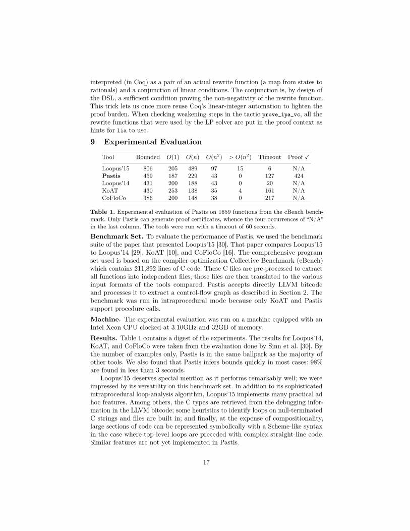
Tool Bounded Op1q Opnq Opn2q ą Opn2

q Timeout Proof X

Loopus’15 806 205 489 97 15 6 N/APastis 459 187 229 43 0 127 424Loopus’14 431 200 188 43 0 20 N/AKoAT 430 253 138 35 4 161 N/ACoFloCo 386 200 148 38 0 217 N/A

Table 1. Experimental evaluation of Pastis on 1659 functions from the cBench bench-mark. Only Pastis can generate proof certificates, whence the four occurrences of “N/A”in the last column. The tools were run with a timeout of 60 seconds.

Benchmark Set. To evaluate the performance of Pastis, we used the benchmarksuite of the paper that presented Loopus’15 [30]. That paper compares Loopus’15to Loopus’14 [29], KoAT [10], and CoFloCo [16]. The comprehensive programset used is based on the compiler optimization Collective Benchmark (cBench)which contains 211,892 lines of C code. These C files are pre-processed to extractall functions into independent files; those files are then translated to the variousinput formats of the tools compared. Pastis accepts directly LLVM bitcodeand processes it to extract a control-flow graph as described in Section 2. Thebenchmark was run in intraprocedural mode because only KoAT and Pastissupport procedure calls.

Machine. The experimental evaluation was run on a machine equipped with anIntel Xeon CPU clocked at 3.10GHz and 32GB of memory.

Results. Table 1 contains a digest of the experiments. The results for Loopus’14,KoAT, and CoFloCo were taken from the evaluation done by Sinn et al. [30]. Bythe number of examples only, Pastis is in the same ballpark as the majority ofother tools. We also found that Pastis infers bounds quickly in most cases: 98%are found in less than 3 seconds.

Loopus’15 deserves special mention as it performs remarkably well; we wereimpressed by its versatility on this benchmark set. In addition to its sophisticatedintraprocedural loop-analysis algorithm, Loopus’15 implements many practical adhoc features. Among others, the C types are retrieved from the debugging infor-mation in the LLVM bitcode; some heuristics to identify loops on null-terminatedC strings and files are built in; and finally, at the expense of compositionality,large sections of code can be represented symbolically with a Scheme-like syntaxin the case where top-level loops are preceded with complex straight-line code.Similar features are not yet implemented in Pastis.

17

From the “Proof X” column, we can see that most but not all the bounds thatPastis generated were successfully checked by Coq. Coq usually processes thegenerated files quickly: 311 files take less than 10 seconds to check, and another83 files take less than 20 seconds. The checking failures are caused by imprecisionin the LP certificates and by our conversion function from floating-point numbersto rational numbers. Especially on higher-degree problems, it is common to see abase function in a loop invariant assigned a small, non-zero, bogus coefficient.Past a certain threshold, our extraction mechanism will output a small rationalnumber when zero is actually needed. On examples with large constants, we alsoobserved LP-solver overflows leading to obviously unsound bounds. As a practicalcounter-measure, our LLVM-bitcode reader replaces all “large” constants withnon-deterministic expressions.

10 Related WorkResource-Bound Analysis. The analysis method presented is based on auto-matic amortized resource analysis (AARA). This analysis technique has beenintroduced for functional programs [17,19,20,33] and has also been applied to de-rive bounds for object-oriented programs [21] and heap-manipulating imperativeprograms [6]. In contrast to our work, none of the previous work focuses on proofcertificates or deriving bounds for imperative code that depend on integers. Mostrelated to our work is the recent application of AARA to derive linear boundsfor imperative integer programs [11]. The main benefits of our work are thederivation of polynomial bounds, the flexibility introduced by rewrite functions,and the automatic verification of resource certificates in Coq.

Amortized analysis has been formalized in the proof assistants Isabelle/HOLand Coq to verify manually the complexity of algorithms and data-structures [14,26]. Our focus is on integer programs rather than sophisticated data-structuresand algorithms, and our technique verifies programs automatically.

Resource-bound analyses that focus on integer programs include CAMPY [31],KoAT [10], Rank [5], CoFloCo [16], COSTA [4] and Loopus [30]. The advantagesof our method include LP-based bound inference, natural compositionality, boundinference for recursive procedures, and automatically-checked Coq certificates.Recent work on an interprocedural analysis that finds procedure summaries innon-linear arithmetic [22] has shown how such information can be used to findresource bounds.

We are only aware of three other papers that describe tools that can generatebounds with machine-verified certificates. Carbonneaux et al. [12] use Coq andthe verified CompCert C compiler to derive stack bounds for assembly code thatare verified by Coq. In contrast to the present paper, their technique does not uselinear constraint solving and automatic verification is limited to constant stackbounds. Blazy et al. [9] describe a loop-bound estimation for WCET analysisthat is formally verified in Coq. An advantage of our method is that we generatecomplex symbolic bounds and can naturally handle recursive functions. Albertet al. [3] have used the KeY program verifier to automatically verify boundsgenerated by the COSTA bound analyzer. While the overall methodology issimilar, we show that we can handle a large set of benchmarks, perform bounds

18

inference via linear programming, and focus on integer bounds rather than boundsthat depend on the sizes of data structures.

Template-Based Methods. Several program-analysis methods use the ideaof (i) choosing a template that characterizes the kind of invariants of a programthat are sought, (ii) extracting an appropriate set of (linear) constraints fromthe program, and (iii) solving the constraints. For example, Template ConstraintMatrices (TCMs) are a parameterized family of linear-inequality domains forexpressing invariants in linear real arithmetic. Sankaranarayanan et al. [27] gavemeet, join, and a set of abstract transformers for all TCM domains. Monniaux [24]gave an algorithm that finds the best transformer in a TCM domain across astraight-line block and good transformers across more complicated control flow.

Müller-Olm and Seidl [25] showed how to obtain invariants that are polynomialequalities of bounded degree. Their method uses a finite-height domain that is avector space whose basis elements are (transformers on) the set of monomials inwhich polynomial invariants can be expressed.

Bagnara et al. [8] presented a technique to generate invariants that arepolynomial inequalities of bounded degree. Their technique introduces additionalvariables (dimensions) to represent nonlinear terms, and uses convex polyhedrato represent polynomial cones in the extended set of variables.

References1. Albert, E., Arenas, P., Genaim, S., Gómez-Zamalloa, M., Puebla, G.: Automatic

inference of resource consumption bounds. In: LPAR (2012)2. Albert, E., Arenas, P., Genaim, S., Puebla, G., Zanardini, D.: Cost analysis of Java

bytecode. In: ESOP (2007)3. Albert, E., Bubel, R., Genaim, S., Hähnle, R., Román-Díez, G.: Verified resource

guarantees for heap manipulating programs. In: FASE (2012)4. Albert, E., Fernández, J.C., Román-Díez, G.: Non-cumulative resource analysis. In:

TACAS (2015)5. Alias, C., Darte, A., Feautrier, P., Gonnord, L.: Multi-dimensional rankings, program

termination, and complexity bounds of flowchart programs. In: SAS (2010)6. Atkey, R.: Amortised resource analysis with separation logic. In: ESOP (2010)7. Avanzini, M., Lago, U.D., Moser, G.: Analysing the complexity of functional

programs: Higher-order meets first-order. In: ICFP (2012)8. Bagnara, R., Rodríguez-Carbonell, E., Zaffanella, E.: Generation of basic semi-

algebraic invariants using convex polyhedra. In: SAS (2005)9. Blazy, S., Maroneze, A., Pichardie, D.: Formal verification of loop bound estimation

for WCET analysis. In: VSTTE (2013)10. Brockschmidt, M., Emmes, F., Falke, S., Fuhs, C., Giesl, J.: Alternating runtime

and size complexity analysis of integer programs. In: TACAS (2014)11. Carbonneaux, Q., Hoffmann, J., Shao, Z.: Compositional certified resource bounds.

In: PLDI (2015)12. Carbonneaux, Q., Hoffmann, J., Ramananandro, T., Shao, Z.: End-to-end verifica-

tion of stack-space bounds for C programs. In: PLDI (2014)13. Cerný, P., Henzinger, T.A., Kovács, L., Radhakrishna, A., Zwirchmayr, J.: Segment

abstraction for worst-case execution time analysis. In: ESOP (2015)14. Charguéraud, A., Pottier, F.: Machine-checked verification of the correctness and

amortized complexity of an efficient union-find implementation. In: ITP (2015)

19

15. Cousot, P., Cousot, R.: Abstract interpretation: A unified lattice model for staticanalysis of programs by construction or approximation of fixpoints. In: POPL(1977)

16. Flores-Montoya, A., Hähnle, R.: Resource analysis of complex programs with costequations. In: APLAS (2014)

17. Hoffmann, J., Das, A., Weng, S.C.: Towards automatic resource bound analysis forOCaml. In: POPL (2017)

18. Hoffmann, J., Hofmann, M.: Amortized resource analysis with polymorphic recursionand partial big-step operational semantics. In: APLAS (2010)

19. Hoffmann, J., Aehlig, K., Hofmann, M.: Multivariate amortized resource analysis.In: POPL (2011)

20. Hofmann, M., Jost, S.: Static prediction of heap space usage for first-order functionalprograms. In: POPL (2003)

21. Hofmann, M., Jost, S.: Type-based amortised heap-space analysis. In: ESOP (2006)22. Kincaid, Z., Breck, J., Forouhi Boroujeni, A., Reps, T.: Compositional recurrence

analysis revisited. In: PLDI (2017)23. Madhavan, R., Kulal, S., Kuncak, V.: Contract-based resource verification for

higher-order functions with memoization. In: POPL (2017)24. Monniaux, D.: Automatic modular abstractions for template numerical constraints.

LMCS 6(3) (2010)25. Müller-Olm, M., Seidl, H.: Precise interprocedural analysis through linear algebra.

In: POPL (2004)26. Nipkow, T.: Amortized Complexity Verified. In: ITP (2015)27. Sankaranarayanan, S., Sipma, H., Manna, Z.: Scalable analysis of linear systems

using mathematical programming. In: VMCAI (2005)28. Serrano, A., López-García, P., Hermenegildo, M.V.: Resource usage analysis of logic

programs via abstract interpretation using sized types. TPLP 14(4-5) (2014)29. Sinn, M., Zuleger, F., Veith, H.: A simple and scalable approach to bound analysis

and amortized complexity analysis. In: CAV (2014)30. Sinn, M., Zuleger, F., Veith, H.: Difference constraints: An adequate abstraction

for complexity analysis of imperative programs. In: FMCAD (2015)31. Srikanth, A., Sahin, B., Harris, W.R.: Complexity verification using guided theorem

enumeration. In: POPL (2017)32. The Coq Development Team: Reference Manual (Version 8.6). https://coq.inria.

fr/distrib/current/refman/index.html33. Vasconcelos, P.B., Jost, S., Florido, M., Hammond, K.: Type-based allocation

analysis for co-recursion in lazy functional languages. In: ESOP (2015)

20