Automated Essay Scoring for English Using Di˙erent Neural ...
41
) Automated Essay Scoring for English Using Dierent Neural Network Models for Text Classification Xindi Deng Uppsala University Department of Linguistics and Philology Master Programme in Language Technology Master’s Thesis in Language Technology, credits November , Supervisor: Eva Peersson, Uppsala University
Transcript of Automated Essay Scoring for English Using Di˙erent Neural ...

)
Automated Essay Scoringfor English Using Di�erentNeural Network Models forText Classification
Xindi Deng
Uppsala University
Department of Linguistics and Philology
Master Programme in Language Technology
Master’s Thesis in Language Technology, 30 ects credits
November 18, 2021
Supervisor:
Eva Pe�ersson, Uppsala University
Abstract
Written skills are an essential evaluation criterion for a student’s creativity,
knowledge, and intellect. Consequently, academic writing is a common part of
university and college admissions applications, standardized tests, and classroom
assessments. However, the task for teachers is quite daunting when it comes
to essay scoring. Then Automated Essay Scoring may be a helpful tool in the
decision-making by the teacher.
There have been many successful models with supervised or unsupervised
machine learning algorithms in the �eld of Automated Essay Scoring. This thesis
work makes a comparative study among various neural network models with
supervised machine learning algorithms, and di�erent linguistic feature combi-
nations. It also proves that the same linguistic features are applicable to more
than one language.
The models studied in this experiment include TextCNN, TextRNN_LSTM, Tex-
tRNN_GRU, and TextRCNN trained with the essays from the Automated Student
Assessment Prize (ASAP) from Kaggle competitions. Each essay is represented
with linguistic features measuring the linguistic complexity. Those features are di-
vided into four groups: count-based, morphological, syntactic and lexical features,
and the four groups of features can form a total of 14 combinations.
The models are evaluated via three measurements: Accuracy, F1 score and
Quadratic Weighted Kappa. The experimental results show that models trained
only with count-based features outperform the models trained using other feature
combinations. In addition, TextRNN_LSTM performs best, with an accuracy of
54.79%, an F1 score of 0.55, and a Quadratic Weighted Kappa of 0.59, which beats
the statistically based baseline models.
Contents
Acknowledgments 4
1 Introduction 5
2 Background 7
2.1 Approaches in Automatic Essay Scoring . . . . . . . . . . . . . . . . . 7
2.2 Linguistic Features for AES Systems . . . . . . . . . . . . . . . . . . . 8
2.3 Overview of Existing Automatic Essay Scoring Systems . . . . . . . . 9
2.3.1 Project Essay Grade . . . . . . . . . . . . . . . . . . . . . . . 9
2.3.2 Intelligent Essay Assessor . . . . . . . . . . . . . . . . . . . . 10
2.3.3 Electronic Essay Rater . . . . . . . . . . . . . . . . . . . . . . 10
2.3.4 Other AES Systems . . . . . . . . . . . . . . . . . . . . . . . . 11
3 Linguistic Features for the AES Models 12
3.1 Text Pre-processing . . . . . . . . . . . . . . . . . . . . . . . . . . . . 12
3.2 Count-based Features . . . . . . . . . . . . . . . . . . . . . . . . . . . 13
3.3 Morphological Features . . . . . . . . . . . . . . . . . . . . . . . . . . 14
3.4 Syntactic Features . . . . . . . . . . . . . . . . . . . . . . . . . . . . . 15
3.5 Lexical Features . . . . . . . . . . . . . . . . . . . . . . . . . . . . . . 16
3.6 Feature Distribution and Storage . . . . . . . . . . . . . . . . . . . . . 16
4 Experimental Methodology 18
4.1 Convolutional Neural Networks . . . . . . . . . . . . . . . . . . . . . 18
4.2 Recurrent Neural Networks . . . . . . . . . . . . . . . . . . . . . . . . 19
4.3 Recurrent Convolutional Neural Networks . . . . . . . . . . . . . . . 20
5 Experimental Setup 22
5.1 Data . . . . . . . . . . . . . . . . . . . . . . . . . . . . . . . . . . . . . 22
5.2 Hyperparameter Settings . . . . . . . . . . . . . . . . . . . . . . . . . 23
5.3 Evaluation Matrix . . . . . . . . . . . . . . . . . . . . . . . . . . . . . 24
6 Results and Analysis 26
6.1 Research Question 1 . . . . . . . . . . . . . . . . . . . . . . . . . . . . 26
6.2 Research Question 2 . . . . . . . . . . . . . . . . . . . . . . . . . . . . 27
6.3 Research Question 3 . . . . . . . . . . . . . . . . . . . . . . . . . . . . 29
7 Conclusion 34
8 Appendix 36
3
Acknowledgments
First of all, I want to express my heartfelt thanks to Eva Pettersson, who supervised the
thesis work. Throughout the whole process, she gives meticulous guidance on topic
selection, thesis framework, and detailed modi�cation, and provides many valuable
suggestions. Besides, I really appreciate Rex Dajun Ruan since he spent time explaining
the extraction of linguistic features. In addition, I also want to thank Yue Feng for
her technique support. Also, I would like to express my gratitude to my family, who
is all the time supporting and encouraging me. Finally, thank you very much to the
examiner for taking time out of his busy schedule to review this thesis work.
4
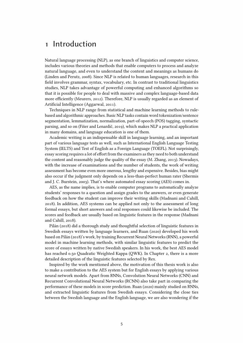
1 Introduction
Natural language processing (NLP), as one branch of linguistics and computer science,
includes various theories and methods that enable computers to process and analyze
natural language, and even to understand the content and meanings as humans do
(Linden and Perutz, 2008). Since NLP is related to human languages, research in this
�eld involves grammar, syntax, vocabulary, etc. In contrast to traditional linguistics
studies, NLP takes advantage of powerful computing and enhanced algorithms so
that it is possible for people to deal with massive and complex language-based data
more e�ciently (Meurers, 2012). Therefore, NLP is usually regarded as an element of
Arti�cial Intelligence (Aggarwal, 2011).
Techniques in NLP range from statistical and machine learning methods to rule-
based and algorithmic approaches. Basic NLP tasks contain word tokenization/sentence
segmentation, lemmatization, normalization, part-of-speech (POS) tagging, syntactic
parsing, and so on (Fišer and Lenardič, 2019), which makes NLP a practical application
in many domains, and language education is one of them.
Academic writing is an indispensable skill in language learning, and an important
part of various language tests as well, such as International English Language Testing
System (IELTS) and Test of English as a Foreign Language (TOEFL). Not surprisingly,
essay scoring requires a lot of e�ort from the examiners as they need to both understand
the content and reasonably judge the quality of the essay (M. Zhang, 2013). Nowadays,
with the increase of examinations and the number of students, the work of writing
assessment has become even more onerous, lengthy and expensive. Besides, bias might
also occur if the judgment only depends on a less-than-perfect human rater (Shermis
and J. C. Burstein, 2003). That’s where automated essay scoring (AES) comes in.
AES, as the name implies, is to enable computer programs to automatically analyze
students’ responses to a question and assign grades to the answers, or even generate
feedback on how the student can improve their writing skills (Madnani and Cahill,
2018). In addition, AES systems can be applied not only to the assessment of long
formal essays, but short answers and oral responses could likewise be included. The
scores and feedback are usually based on linguistic features in the response (Madnani
and Cahill, 2018).
Pilán (2018) did a thorough study and thoughtful selection of linguistic features in
Swedish essays written by language learners, and Ruan (2020) developed his work
based on Pilán (2018)’s work, by training Recurrent Neural Networks (RNN), a powerful
model in machine learning methods, with similar linguistic features to predict the
score of essays written by native Swedish speakers. In his work, the best AES model
has reached 0.50 Quadratic Weighted Kappa (QWK). In Chapter 2, there is a more
detailed description of the linguistic features selected by Rex.
Inspired by the work mentioned above, the motivation of this thesis work is also
to make a contribution to the AES system but for English essays by applying various
neural network models. Apart from RNNs, Convolution Neural Networks (CNN) and
Recurrent Convolutional Neural Networks (RCNN) also take part in comparing the
performance of these models in score prediction. Ruan (2020) mainly studied on RNNs,
and extracted linguistic features from Swedish essays. Considering the close ties
between the Swedish language and the English language, we are also wondering if the
5
same set of linguistic features are still practical in English AES systems, and how the
CNN and RCNN can perform. All these purposes lead to three main research questions:
• What results could be achieved for automatic essay scoring for English, using
similar linguistic features as have previously been used for Swedish?
• Which linguistic features or feature combinations are most essential for English
AES systems?
• Will neural networks with a convolutional architecture better optimize the AES
models when compared with the RNN models?
We look forward to seeing if the neural network models can assign the right score
to the essay, or in other words to classify the essay into the right score category. The
so-called "right sore" is the score given by human raters regardless of bias or other
issues.
In the next chapter, we give a background to AES research and studies, including
existing AES systems, relevant models and algorithms, a diverse variety of linguistic
features selected by di�erent researchers, as well as the commonly used evaluation
matrix for AES systems. Chapter 3 mainly lists the linguistic features used in this thesis
work, and how they are di�erent from Rex’s. Chapter 4 provides a basic description of
the neural network models used in this experiment. Chapter 5 is about the data and
hyperparameters for di�erent models. The �nal results are presented in Chapter 6,
where we also give answers to the research questions listed in this chapter, along with
an analysis and evaluation of the results. The last chapter is a brief summary of all the
work.
6
2 Background
Though with numerous experiment results and systems proposed, AES is still a di�cult
and interesting issue in AI and NLP (Walia et al., 2019), and Page is generally considered
the pioneer of this task (J. Wang and Brown, 2007). As early as 1966, Page started his
work from the design of the Project Essay Grader system (PEG), and prophesied that
AES systems would come as a “teacher’s helper” someday. He applied multiple linear
regression models trained with textual features extracted from the texts, and identi�ed
some powerful and predictive linguistic features, such as word length, text length, the
number of low-frequency words, etc. (J. Wang and Brown, 2007). From then to the last
few decades, AES has been developing rapidly. In this chapter, we provide a review of
AES systems, in terms of methodologies, linguistic features, and some well-known
systems that are already in use.
2.1 Approaches in Automatic Essay Scoring
For several decades, researchers have been exploring various techniques for the de-
velopment of AES systems, from rule-based and statistical methods to more updated
neural network models for di�erent tasks. The advantage of rule-based methods is that
it is easy to integrate domain knowledge into language knowledge, which provides
highly accurate results (Walia et al., 2019). The rules could be for Agreement which
requires linguistic features such as part-of-speech or syntactic parsing. A more speci�c
rule, as for Capitalization, is based on regular expressions to detect block capitals, or
the rule for Apology, which is a theme of a certain writing task, focuses on speci�c
lexical entities like ‘sorry’, ‘apologies’ and etc.(Crowston et al., 2010). Some statistically
based classi�ers that are commonly used in AES studies include, for example, Linear
Regression (Crossley et al., 2015; Klebanov et al., 2016; Page, 1966), Support Vector
Machine (SVM) (Cozma et al., 2018; Persing and V. Ng, 2015), Sequential Minimal
Optimization (SMO), which is a a variant of SVM (Vajjala, 2018), Bayesian network
(Rudner and Liang, 2002), and so forth.
Almost all the models above have to focus on feature engineering, counting on
carefully designed linguistic features so that the systems can evaluate or score essays
better. However, Taghipour and H. T. Ng (2016) criticized the unfriendly and laborious
work of the hand-crafted feature engineering. On account of that, deep learning in
neural networks has become a hot topic in AES studies since they make it possible
to get rid of the manual feature extraction (Alikaniotis et al., 2016; Taghipour and
H. T. Ng, 2016; Uto and Okano, 2020; Y. Wang et al., 2018).
Taghipour and H. T. Ng (2016) developed a system based on RNNs to learn the
relation between an essay and the score assigned to it without feature engineering.
The RNN architecture used in his experiment included four important layers: the
lookup table layer encoded each word in the essay with its one-hot representation
or embedding; the convolution layer was used to extract local n-gram level features;
the recurrent layer took as input those features and output a vector or generated
representations for the whole essay in other words at each time step; and �nally the
dense layer received the vectors and was responsible for predicting the score. They had
expected that long essays might cause problems for the learned vector representation.
Therefore, they preserved all the intermediate states to keep track of the important
7
bits of information. They examined vanilla RNN, and two other variant models, Gated
Recurrent Unit (GRU) and Long Short-Term Memory (LSTM), and found out that the
performance of LSTM was signi�cantly better than all other systems with a 0.75 QWK
score. Their results also proved that the absence of feature engineering had little e�ect
on the neural network models. All the RNN variations achieved higher QWK scores
than Enhanced AI Scoring Engine (EASE), which is a statistically based AES system.
Although the researchers still could not explain in detail what speci�c features were
actually learned by the RNN models, their results showed that the features could be
learned properly, no matter if length-based or content-based features were used.
Z. Chen and Zhou (2019) implemented a combination of CNN + ordinal regres-
sion(OR) model and tried evaluating the model on the corpus from the ASAP compe-
tition organized by Kaggle1. The motivation of the work was also to design a more
robust model without manual feature extraction. CNN consisting of multiple di�erent
layers was used as a feature learner. The convolutional layer was used to extract feature
vectors from n-grams. The fully connected layer retained those highly puri�ed features
that facilitated the �nal OR operation. In this layer, the data from the upper layer was
converted into one-dimensional vectors, multiplied by the weight matrix, plus the
o�set, and the Sigmoid activation function was used. Afterward, the OR architecture
was applied to the output data to solve some order relationship between categories,
which makes the output data more realistic and logical so that the system can make
better predictions. Their results showed that the AES system based on CNN+OR had a
high accuracy on the ASAP dataset and a better QWK score of 0.826.
However, some other researchers suggested a combination of neural networks
and feature engineering (J. Liu et al., 2019). Dong et al. (2017) mentioned that neural
network models usually performed better with hand-crafted features than those with-
out. Dasgupta et al. (2018), instead of word and sentence features, proposed complex
linguistic, cognitive and psychological features along with a hierarchical CNN and
bidirectional LSTM model. More information on these features is given in the next
section. The experiment result showed a good QWK of around 0.80. What’s more,
their model surpassed other neural network models in terms of Pearson’s correlation
and Spearman’s ranking correlation, which were 0.94 and 0.97 respectively compared
to 0.91 and 0.96 in Alikaniotis et al. (2016)’s model without feature engineering. As
Ke and V. Ng (2019) said, feature-based approaches and neural networks should not
be competing but complementary approaches. Considering the limited and small-size
dataset of natural languages even for English, manual extraction of text features still
needs to be maintained.
2.2 Linguistic Features for AES Systems
As mentioned in previous sections, feature engineering still plays an important part
in the training of both statistically based models and neural models. Obviously, the
performance of AES models has a lot to do with the selection of features.
Most of the features are selected from the perspective of linguistics. Length-based
or count-based features are one of the most commonly used linguistic features for
AES systems since they were found to be highly positively correlated with the overall
score of an essay (Ke and V. Ng, 2019). Features in this type may include word length,
sentence length, the number of tokens, the number of long words, and so on.
Features related to lexis can be the number of occurrences of particular n-grams,
like verb phrases, out of vocabulary (OOV) words (Ruan, 2020), or types of punctuation
1The website of the Automated Student Assessment Prize (ASAP): https://www.kaggle.com/c/asap-
aes/overview
8

in an essay (Phandi et al., 2015). Lexical features can also include word level features.
These are usually computed based on a word list or a dictionary. H. Chen and He
(2013) referred to Webster dictionary, and divided the words into 8 levels according to
the College Board Vocabulary Study (Breland et al., 1994). The higher the level of the
word, the lower the frequency of the word. Then words like thoroughfare is classi�ed
into level 8, and words with a similar meaning like passage belong to a lower level of
category.
Syntactic features are usually extracted from parse trees, showing all head-dependent
pairs in a sentence. Features could include a ratio of a particular phrase structure or
clause to represent grammatical constructions, or the syntactic structure of a sentence
can be detected by looking for the depth of the parse tree (H. Chen and He, 2013).
Apart from linguistic features, Dasgupta et al. (2018) made use of psychological
features which were mostly derived from the Linguistic Inquiry and Word Count
(LIWC) tool (Tausczik and Pennebaker, 2010). Word choice can re�ect a person’s
perception. For example, the number of �rst-person singular pronouns can re�ect the
writers’ su�ering in physical or emotional pain. The tendency to use a lot of past tense
means more inclined to focus on the past. The emotion in use can also be identi�ed by
positive emotion words and negative emotion words.
Ruan (2020) in his work extracted 63 linguistic features, and divided them into four
blocks. Picture 2.1 below shows all the features in his work. Since his models trained
with these features showed good results, and the features are at the same time easy to
implement, we use them as a reference in our work and modify them a little bit so as
to �t the English language better.
Figure 2.1: Linguistic features described by Ruan (2020)
2.3 Overview of Existing Automatic Essay Scoring Systems
2.3.1 Project Essay Grade
Project Essay Grade (PEG), developed by Ellis Page together with other colleagues
in the 1960s, is the �rst AES system (Page, 2003), and also one of the longest-lived
9

implementations (Valenti et al., 2003). It relies purely on a statistical approach, almost
without any natural language processing techniques (Ghanta, 2019). The statistical
approach is re�ected in the extraction and style analysis of surface linguistic features.
According to Valenti et al. (2003), the design for PEG is mostly based on two im-
portant concepts:trins and proxes. Trins are variables that can be directly seen by
human raters but can not be directly gained by computers, while proxes can be directly
acquired by computers and used to estimate trins. For example, some measurable
features included in proxes, such as essay length, is to represent the trin of �uency, and
the number of prepositions, relative pronouns, etc. are used to indicate the complexity
of sentence structure. All the proxes calculated from the training dataset are vectorized
via a standard multiple regression along with the human grades so that the regression
coe�cients can be obtained. The regression coe�cients represent the weight of proxes
in manual scoring.
Despite the great contribution to AES studies, there are still some limitations of
PEG. On the one hand, PEG mainly focuses on surface linguistic features but ignores
content-based features of an essay. On the other hand, the system is vulnerable. It is
possible to trick the system with longer but low text quality essays (Dikli, 2006).
2.3.2 Intelligent Essay Assessor
Another classic AES system is Intelligent Essay Assessor (IEA), which was developed
by Hearst (2000). Di�erent from PEG, IEA is a content-based AES system that uses
the Latent Semantic Analysis (LSA) to score content quality (Landauer and Kintsch,
2003). Its core idea can be summarized as the meaning of an essay is the sum of the
meanings of each word in it (Landauer and Kintsch, 2003).
LSA is a machine learning method which can represent the content of an essay in
a two-dimensional matrix (Valenti et al., 2003). Each row in this matrix presents a
word, each column represents the context where the word occurs, and each cell value
in the matrix acts for the word frequency. Singular Value Decomposition (SVD), a
matrix algebra technique, is applied to decompose the matrix into three smaller-sized
matrices (Landauer and Kintsch, 2003). The three matrices work to reform the original
matrix when multiplied together so that the hidden relations between the essay and
the words in it can be obtained (Valenti et al., 2003).
To sum up, in order to grade an essay, a matrix about the essay is �rst established,
and then SVD is employed to reproduce the matrix representing the content of the
essay. Finally, cosine correlation is used to measure the content similarity between a
"model answer" and this essay.
IEA can be used to score essays of a variety of di�erent themes. Its disadvantage is
the loads of calculation time of LSA due to the large size of the matrix (Valenti et al.,
2003).
2.3.3 Electronic Essay Rater
The PEG system scores essays is based on accurately extracted proxes that re�ect
the grammatical quality and vocabulary accuracy, and IEA uses LSA to feedback the
quality of the content. Electronic Essay Rater (E-rater), developed by J. Burstein et al.
(2001), takes both the structure and content into consideration.
The E-rater system combines statistical methods and NLP techniques to extract
linguistic features. Syntactic features, such as di�erent types of subordinate clauses
and subjunctive modal auxiliary verbs, are identi�ed by means of the MsNLP tool. The
automated argument partitioning and annotation a program (APA) was implemented
to analyze the discourse structure of each essay. When it comes to topical analysis,
10
word frequency and word weight were used to evaluate the topical content of an
essay, by comparing the words the essay contained to their counterparts found in the
manually scored training set.
Compared with other systems, E-Rater is far more complicated and thus requires
more training. What’s more, there is neither a downloadable trial version nor an
on-line demonstration, which makes E-rater hard to be accessed (Valenti et al., 2003).
2.3.4 Other AES Systems
IntelliMetric, developed by Vantage learning company since 1998, can extract more
than 300 features, including variables such as semantic features, syntactic features, and
features relating to the theme. It extracts features from the following �ve dimensions:
whether the central idea meets the requirements of the topic, the integrity of the article
(measured by whether the content of the essay is compact), the organization of the
essay (the logic of the argument), sentence structure, and whether it conforms to the
rules of standard written English.
Elliot and Mikulas (2004) provide a su�cient amount of insight into the IntelliMetric
system. The text is parsed to indicate the syntactic and grammatical structures of the
essay. Each sentence is tagged according to POS, vocabulary, sentence structure, and
conceptual expression. Then the text is examined by a number of patented technologies,
including morphological analysis, spell checking, grammatical collocation, and so on.
Instead of the multiple regression model employed by PEG and E-rater, IntelliMetric
uses a non-linear and multi-dimensional learning model associating with the features
to yield a single assigned score for each essay (Rudner et al., 2006).
Bayesian Essay Test Scoring System (BETSY), developed by Lawrence and Liang
(Rudner and Liang, 2002) at the College Park of the University of Maryland, is a
program based on text classi�cation. The system aims to determine the most likely
classi�cation of an essay into a four-point scale. Features including both content and
style speci�c issues are used for the classi�cation (Valenti et al., 2003). According
to Rudner and Liang (2002), two underlying models are employed in the system
to compute the product of the probabilities of the features contained in the essay,
along with the conditional probability of presence of each feature. Though simple to
implement, BETSY usually needs a long time to process the data since every term in
the vocabulary has to be examined. Besides, di�erent from E-rater, BETSY is a freely
downloadable software.
11

3 Linguistic Features for the AES Models
It is necessary to formalize the text �rst to facilitate computer processing. Ruan (2020)
in his work used a template of linguistic features, which has been listed in �gure 2.1,
to represent the essays with tensors as the input of his models. The aim of his models
was to predict the score of essays written by native Swedish students. Considering
that we also use the essays written by �rst language speakers as data, the linguistic
features pointed up by Ruan (2020) can be a good starting point. Therefore, our AES
models are also trained with the linguistic features similar to Ruan (2020)’s for the
reason that English and Swedish share many features. In this chapter, we mainly talk
about the linguistic features used for model training, and point out the di�erence from
Ruan (2020)’s choices.
3.1 Text Pre-processing
Data pre-processing is a data mining technique that involves converting raw data into
a format that is more easily interpretable by a computer. The general outline of data
pre-processing for this experiment includes word tokenization, sentence segmentation,
normalization, lemmatization, part-of-speech tagging, and syntactic parsing. Tokeniza-
tion is the division of a text string into smaller pieces, or "tokens". Paragraphs can be
segmented into sentences and sentences can be tokenized into words (Mayo, 2017).
Further processing is usually conducted upon appropriate tokenization of a chunk
of text. Normalization refers to a series of related tasks putting all tokens on equal
footing (Mayo, 2017). In our experiment, normalization includes converting all text to
the lower case and spell checking. Lemmatization is the process of converting a word
into its base form, like dancing to dance, best to good. Part-of-speech-tagging is to tag
each word grammatically. The word is labeled as a noun, a verb, an adjective and so
forth. Syntactic parsing is to analyze the grammatical structure of a text.
ID NORM FORM LEMMA32 helps helps help
UPOS XPOS FEATS HEAD
VERB VBZ
Number=Sing|Person=Three|
Tense=Pres|VerbForm=Fin
helps
HEAD IDX DEPREL0 ROOT
Table 3.1: A word line example in the text file
Both sentence segmentation and word tokenization are carried out by the sub-
modules in Python NLTK. The rest of the procedures, which are normalization, lemma-
tization, part-of-speech tagging, and syntactic parsing, are conducted by spaCy.1
spaCy
is a library for advanced NLP in Python and Cython. It comes with pre-trained pipelines
for more than 60 languages and features state-of-the-art models that can be used for
almost all NLP tasks, such as tagging, parsing, text classi�cation, and so on. With
1see the website of spaCy: https://spacy.io/
12

spaCy, the cumbersome steps can be easily completed. The pre-processed data is stored
in a text �le, and each line consists of necessary information of every single word.
Table 3.1 is an example of one-word line.
We take helps as an example. UPOS and XPOS refer to Universal part-of-speech tags
and Language-speci�c part-of-speech tags. FEATS lists the morphological features of
helps. The features in Table 3.1 mean that helps is a 3rd person singular �nite verb in
the present tense. HEAD refers to the head of helps, which is itself, so the DEPREL
(Universal dependency relation) is ROOT, and the ID value of ROOT is zero.
Inspired by Ruan (2020)’s work, we also extract linguistic features from four aspects,
which are count-based, morphological, syntactic, and lexical features respectively. In
the next few sections, we introduce all the features in the order mentioned above.
3.2 Count-based Features
It is not hard to understand that count-based features refer to super�cial features or
surface variables of a text, which is a simple but powerful way to �nd information
about an essay in almost any language. Table 3.2 lists all the count-based features
employed in our experiment.
Count-based FeaturesNo.Character in Token No. Character in Type
No. Tokens No.Long Tokens
No.Types No.Long Types
Avg.Token Length Avg.Type Length
No. Misspellings No. Sentence
No. Paragraph Bi-logarithm TTR
Square Root TTR
Table 3.2: Count-based features
The features adopted in this project comprise the number and the average length
of words, sentences, and types per essay, by which type means words that are only
counted once. For instance, there are eleven words in the sentence The features of thesetting a�ected the cyclist in many ways, but the number of types is nine since the
de�nite article (the) is only counted as one even though it appears three times.
Besides, the number of POS tags, as well as long tokens and long types are also
included. The de�nition of long tokens here is di�erent from that in Ruan (2020)’s
work. According to Tausczik and Pennebaker (2010), words greater than six letters
indicate a more complex English. Therefore, we treat tokens that consist of more than
6 characters as long tokens or types for English instead of 13 characters which is for
Swedish.
Another di�erence is the removal of Lix in our experiment since it is used to measure
the readability of Swedish. As stated in the work of Falkenjack et al. (2013), readability
metrics for English consists of those count-based features such as average word length,
lexical variation, and frequency of "simple words". Considering these features are
already included in our scoring function, we give up the adoption of a speci�c function
to calculate the readability of English.
The proportion of misspellings is taken as one of the count-based features too.
Misspellings refer to incorrectly spelled words that can be found if the FORM of the
word di�ers from the NORM of the word.
13
Type Token Ratio (TTR) is an e�ective measure to evaluate richness or variety in
vocabulary. A simple TTR is the total number of types divided by the total number of
tokens in a given language segment. Inspired by Ruan (2020)’s work, bi-logarithm TTR
and square root TTR are calculated and implemented based on the equations below.
5 (Bi-logarithm TTR) = ln (Counts(type))
ln (Counts(token))
(3.1)
5 (Square Root TTR) = Counts(type)√Counts(token)
(3.2)
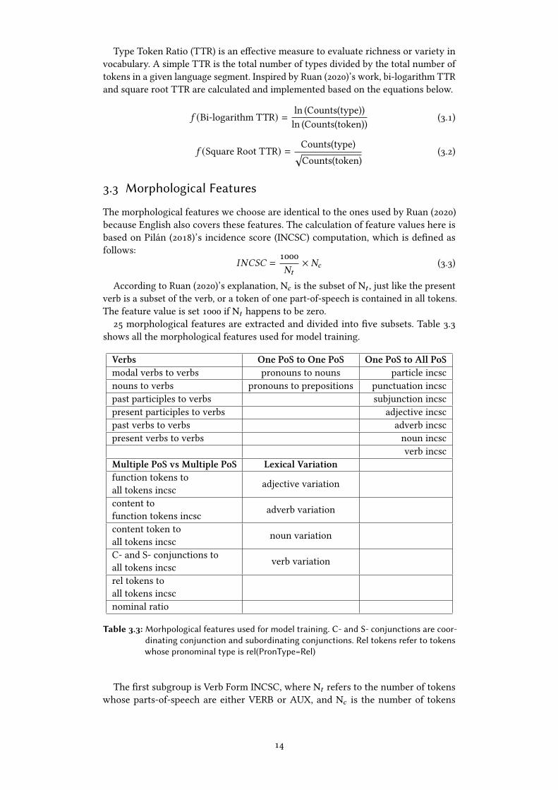
3.3 Morphological Features
The morphological features we choose are identical to the ones used by Ruan (2020)
because English also covers these features. The calculation of feature values here is
based on Pilán (2018)’s incidence score (INCSC) computation, which is de�ned as
follows:
�#�(� =1000
#C× #2 (3.3)
According to Ruan (2020)’s explanation, N2 is the subset of NC , just like the present
verb is a subset of the verb, or a token of one part-of-speech is contained in all tokens.
The feature value is set 1000 if NC happens to be zero.
25 morphological features are extracted and divided into �ve subsets. Table 3.3
shows all the morphological features used for model training.
Verbs One PoS to One PoS One PoS to All PoSmodal verbs to verbs pronouns to nouns particle incsc
nouns to verbs pronouns to prepositions punctuation incsc
past participles to verbs subjunction incsc
present participles to verbs adjective incsc
past verbs to verbs adverb incsc
present verbs to verbs noun incsc
verb incsc
Multiple PoS vs Multiple PoS Lexical Variationfunction tokens to
all tokens incsc
adjective variation
content to
function tokens incsc
adverb variation
content token to
all tokens incsc
noun variation
C- and S- conjunctions to
all tokens incsc
verb variation
rel tokens to
all tokens incsc
nominal ratio
Table 3.3: Morhpological features used for model training. C- and S- conjunctions are coor-
dinating conjunction and subordinating conjunctions. Rel tokens refer to tokens
whose pronominal type is rel(PronType=Rel)
The �rst subgroup is Verb Form INCSC, where NC refers to the number of tokens
whose parts-of-speech are either VERB or AUX, and N2 is the number of tokens
14
belonging to one of the following categories: modal verbs, nouns, past participles,
present participles, past verbs, as well as present verbs. For example:
�#�(� (modal verbs to verbs) = 1000
verbs
×modal verbs (3.4)
In the subgroup of One PoS to One PoS, NC and N2 are stated for a pair of di�erent
parts of speech, which are pronouns to nouns, and pronouns to prepositions in this
experiment.
NC in the One PoS to All PoS group includes all tokens, while N2 is the number of
tokens from one of the seven categories: particle, punctuation, subjunction, adjective,
adverb, noun, and verb.
We also check function tokens and content tokens. Words in language can tradi-
tionally be classi�ed as either content or function words (Biber and Finegan, 2008;
Rayner et al., 2012). Content words always have meaning, while function words are
used to explain or create grammatical or structural relationships for content words.
The content or open-class parts-of-speech cover nouns, most verbs, adjectives, most
adverbs, proper nouns, and interjections. Those closed-class ones could be adpositions,
auxiliary verbs, coordinating conjunctions, subordinating conjunctions, determiners,
numerals, particles, pronouns, punctuations, symbols, and others. Therefore, in the
group of Multiple PoS vs Multiple PoS, it is not hard to understand what N2 and NC
stand for based on the name of the features. Pilán, 2018 also has nominal ratio as a
morph feature, where N2 is made up of nouns, adpositions, and participles, and NC
consists of pronouns, verbs and adverbs.
In the last group, N2 is the number of adjectives, adverbs, nouns, and verbs re-
spectively, divided by NC that refers to all tokens from the four classes above. For
example:
�#�(� (verb variation) = 1000
adjectives+adverbs+nouns+verbs
× verbs (3.5)
3.4 Syntactic Features
As mentioned in section 3.1, spaCy can be used for the syntactic annotation so that it
is very convenient for us to obtain all dependent-head pairs and the corresponding
syntactical relationships of a sentence. Instead of head and dependent, the spaCy
pipeline uses the terms head and child to represent the words connected by a single
arc in the dependency tree. Every arc has a label, which is DEPREL, to describe the
type of syntactic relation that connects the child to the head.
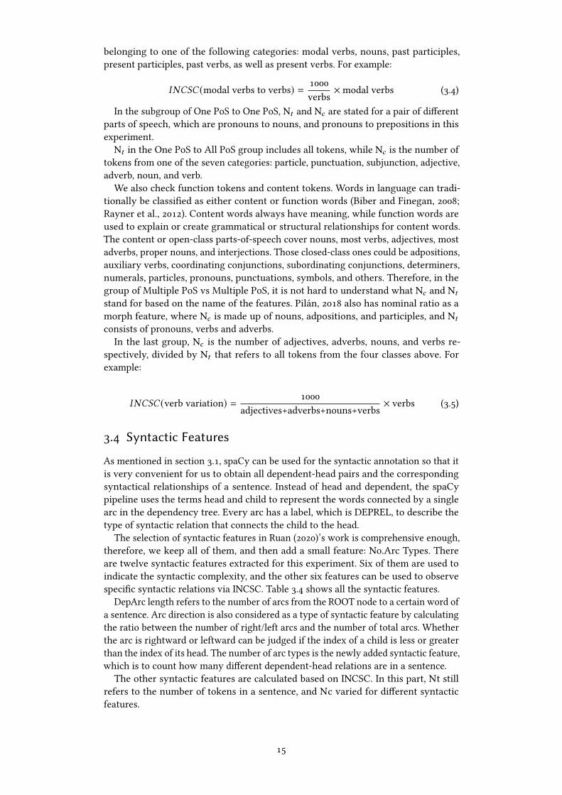
The selection of syntactic features in Ruan (2020)’s work is comprehensive enough,
therefore, we keep all of them, and then add a small feature: No.Arc Types. There
are twelve syntactic features extracted for this experiment. Six of them are used to
indicate the syntactic complexity, and the other six features can be used to observe
speci�c syntactic relations via INCSC. Table 3.4 shows all the syntactic features.
DepArc length refers to the number of arcs from the ROOT node to a certain word of
a sentence. Arc direction is also considered as a type of syntactic feature by calculating
the ratio between the number of right/left arcs and the number of total arcs. Whether
the arc is rightward or leftward can be judged if the index of a child is less or greater
than the index of its head. The number of arc types is the newly added syntactic feature,
which is to count how many di�erent dependent-head relations are in a sentence.
The other syntactic features are calculated based on INCSC. In this part, Nt still
refers to the number of tokens in a sentence, and Nc varied for di�erent syntactic
features.
15
Syntactic Complexity Speci�c Syntactic RelationsAvg. DepArc Length Pre-modi�er INCSC
Max DepArc Length Post-modi�er INCSC
NO. DepArc Length 5+ Modi�er Variation
Right DepArc Ratio Subordinate INCSC
Left DepArc Ratio Rel Clause INCSC
No. Arc Types PREP Comp INCSC
Table 3.4
A modi�er refers to the dependent whose dependent-head relation is labeled with
nmod, appos, nummod, advmod, discourse or amod. Therefore, pre- and post-modi�er
refer to such dependent coming before or after its head. Modi�er variation consists of
both pre- and post-modi�ers. Nc here refers to the number of modi�ers.
Subordinate refers to the head and dependent if their relation is labeled with csubj,xcomp, ccomp, advcl, acl or acl:relcl. Relative Clause INCSC can be obtained by counting
the number of dependents whose FEATS include PronType=Rel. Similarly, the calcula-
tion of PREP Comp INCSC requires the number of dependents whose dependent-head
arc is annotated with case.
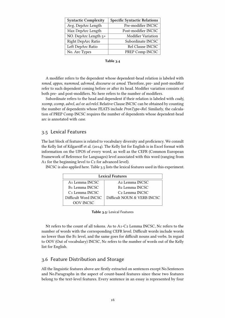
3.5 Lexical Features
The last block of features is related to vocabulary diversity and pro�ciency. We consult
the Kelly list of Kilgarri� et al. (2014). The Kelly list for English is in Excel format with
information on the UPOS of every word, as well as the CEFR (Common European
Framework of Reference for Languages) level associated with this word (ranging from
A1 for the beginning level to C2 for advanced level).
INCSC is also applied here. Table 3.5 lists the lexical features used in this experiment.
Lexical FeaturesA1 Lemma INCSC A2 Lemma INCSC
B1 Lemma INCSC B2 Lemma INCSC
C1 Lemma INCSC C2 Lemma INCSC
Di�cult Word INCSC Di�cult NOUN & VERB INCSC
OOV INCSC
Table 3.5: Lexical Features
Nt refers to the count of all tokens. As to A1-C2 Lemma INCSC, Nc refers to the
number of words with the corresponding CEFR level. Di�cult words include words
no lower than the B1 level, and the same goes for di�cult nouns and verbs. In regard
to OOV (Out of vocabulary) INCSC, Nc refers to the number of words out of the Kelly
list for English.
3.6 Feature Distribution and Storage
All the linguistic features above are �rstly extracted on sentences except No.Sentences
and No.Paragraphs in the aspect of count-based features since these two features
belong to the text-level features. Every sentence in an essay is represented by four
16
lists storing four kinds of linguistic features. Since the number of sentences is varied
from essay to essay, we calculate an average value so that the number of features in
each essay is consistent.
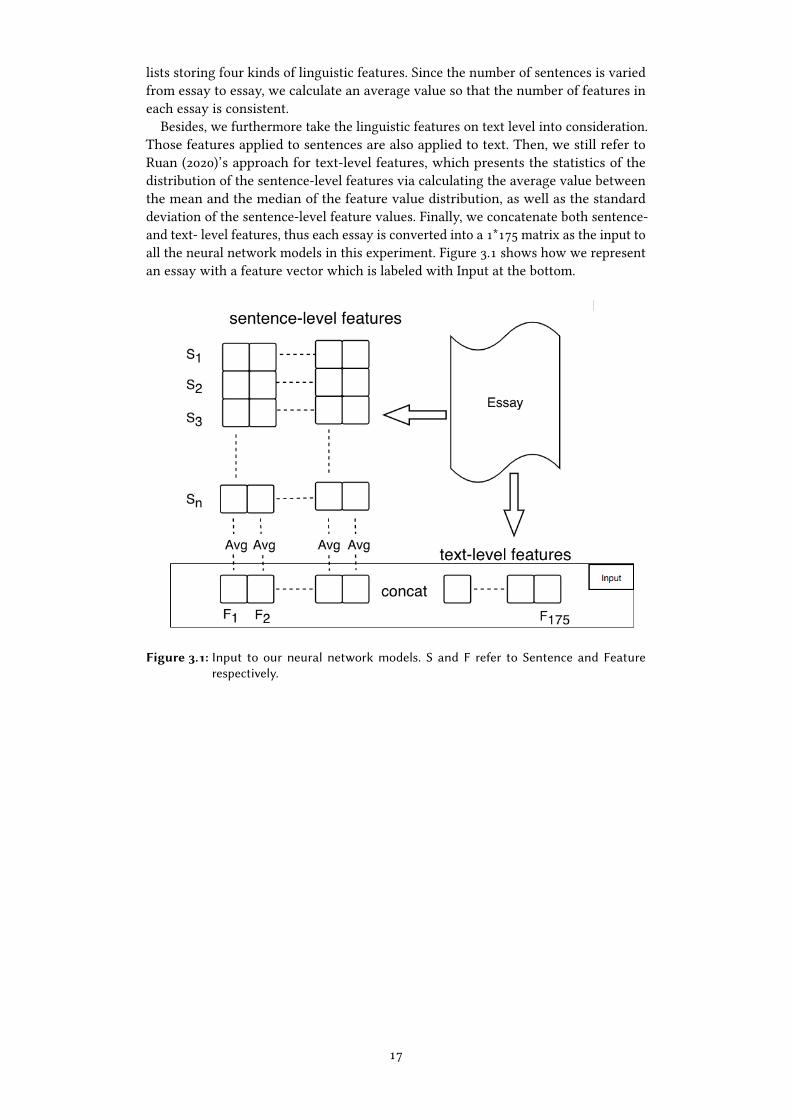
Besides, we furthermore take the linguistic features on text level into consideration.
Those features applied to sentences are also applied to text. Then, we still refer to
Ruan (2020)’s approach for text-level features, which presents the statistics of the
distribution of the sentence-level features via calculating the average value between
the mean and the median of the feature value distribution, as well as the standard
deviation of the sentence-level feature values. Finally, we concatenate both sentence-
and text- level features, thus each essay is converted into a 1*175 matrix as the input to
all the neural network models in this experiment. Figure 3.1 shows how we represent
an essay with a feature vector which is labeled with Input at the bottom.
Figure 3.1: Input to our neural network models. S and F refer to Sentence and Feature
respectively.
17

4 Experimental Methodology
As mentioned in the introduction, the neural network models deployed in this experi-
ment include TextRNN_LSTM/GRU, TextCNN, and TextRCNN. In this chapter, each
one of the models will be introduced.
4.1 Convolutional Neural Networks
TextCNN, proposed by Kim (2014) as a �ne-tuned CNN model, has a very useful and
e�ective learning algorithm for short text classi�cation tasks. According to Kim (2014),
the model architecture is a slight variant of the CNN architecture of Collobert et al.
(2011). Figure 4.1 from the work of Y. Zhang and Wallace (2015) shows the model
architecture for an example sentence.
Figure 4.1: TextCNN architecture for sentence classification (Y. Zhang and Wallace, 2015)
TextCNN uses pre-trained word embeddings as the input embedding layer. As each
word in the sentence can be represented as a vector, we get an embedding matrix
18
� × # , where D represents the embedding dimension, and N refers to the number
of tokens. The matrix can be static (�xed), or non-static which is updated based on
backpropagation, or applies two channels for being both static and non-static.
This matrix then comes to the one-dimensional convolutional layer, and the size of
each convolution kernel is � × � , where F is a hyperparameter (�lter size in table 5.3)
that can be set. Convolution kernels of di�erent sizes (F = 2,3,4 in �gure 4.1) are also
used to extract features of di�erent text lengths. A feature map c = [21, 22, . . . , 2#−�+1]is generated by convolving the words in the sentence for each possible kernel size.
The size of the feature map obtained with di�erent sizes of convolution kernels
is also di�erent. The pooling function is used to make each feature map in the same
dimension. 1-max pooling is the most commonly used. It can extract the maximum
value, which is the most important feature, of each feature map so that there is only
one value for each convolution kernel. Apply 1-max pooling for all convolution kernels,
and then concatenate them together to get the �nal feature vector, which is then input
into the Dropout and Softmax layer for classi�cation.
The TextCNN implemented in our experiment is derived from the model designed
by Y. Zhang and Wallace (2015). We employ CNN-non-static for training since it
performed the best on data with �ne-grained labels (Kim, 2014), which is similar to
our data. One thing worth noting is that the input of our models is the feature vector
(see section 3.6) of an entire essay, rather than word embeddings as what Y. Zhang and
Wallace (2015) did. The speci�c hyperparameters for our TextCNN model are listed in
table 5.3.
4.2 Recurrent Neural Networks
TextRNN (P. Liu et al., 2016) is a bi-directional RNN so that bi-directional "n-grams"
with variable length can be captured (Cai et al., 2018). Considering vanilla RNNs may
cause vanishing gradient problem when processing long texts, we exploit the variants
TextRNN_LSTM (bi-directional LSTM) or TextRNN_LSTM (bi-directional GRU) for
the classi�cation.
Our LSTM model assigns a separate LSTM layer on the basis of BiLSTM, then
concatenates the hidden states of the BiLSTM at each time step as an input of the
upper separate LSTM. Finally, apply the last hidden state of the separate LSTM to the
softmax layer, and the classi�cation result is obtained.
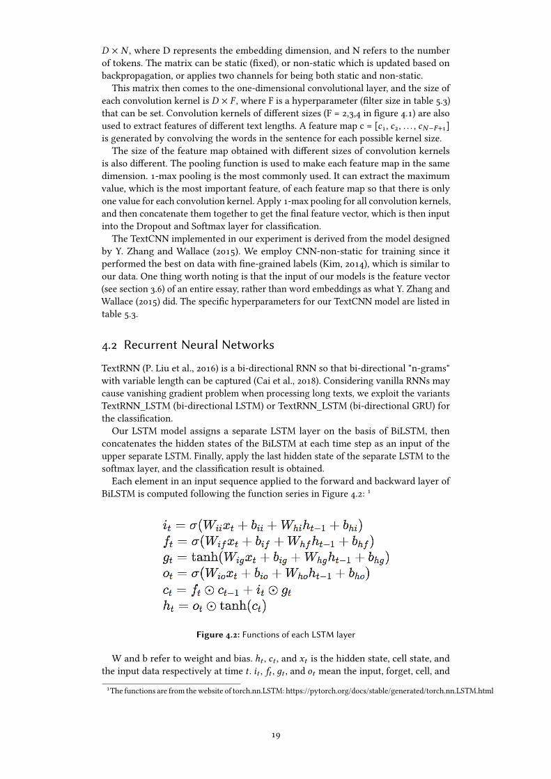
Each element in an input sequence applied to the forward and backward layer of
BiLSTM is computed following the function series in Figure 4.2:1
Figure 4.2: Functions of each LSTM layer
W and b refer to weight and bias. ℎC , 2C , and GC is the hidden state, cell state, and
the input data respectively at time C . 8C , 5C , 6C , and >C mean the input, forget, cell, and
1The functions are from the website of torch.nn.LSTM: https://pytorch.org/docs/stable/generated/torch.nn.LSTM.html
19
output gates. ℎC−1 refers to the hidden state at previous time step and ℎ0 is the initial
hidden state. f and � are the sigmoid function and the Hadamard product.
The input of the separate LSTM layer is the product of the concatenated hidden
states of the BiLSTM multiplied by dropout. The product in this layer is processed
with the same functions in Figure 4.2.
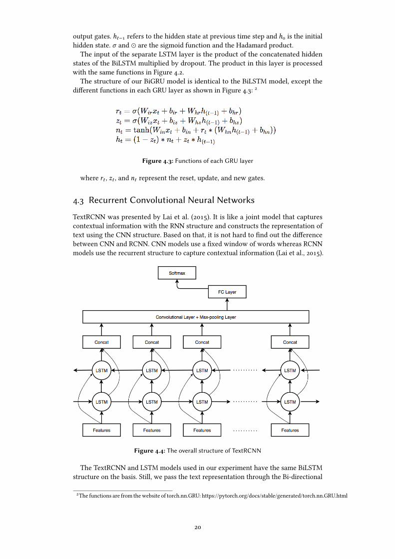
The structure of our BiGRU model is identical to the BiLSTM model, except the
di�erent functions in each GRU layer as shown in Figure 4.3:2
Figure 4.3: Functions of each GRU layer
where AC , IC , and =C represent the reset, update, and new gates.
4.3 Recurrent Convolutional Neural Networks
TextRCNN was presented by Lai et al. (2015). It is like a joint model that captures
contextual information with the RNN structure and constructs the representation of
text using the CNN structure. Based on that, it is not hard to �nd out the di�erence
between CNN and RCNN. CNN models use a �xed window of words whereas RCNN
models use the recurrent structure to capture contextual information (Lai et al., 2015).
Figure 4.4: The overall structure of TextRCNN
The TextRCNN and LSTM models used in our experiment have the same BiLSTM
structure on the basis. Still, we pass the text representation through the Bi-directional
2The functions are from the website of torch.nn.GRU: https://pytorch.org/docs/stable/generated/torch.nn.GRU.html
20
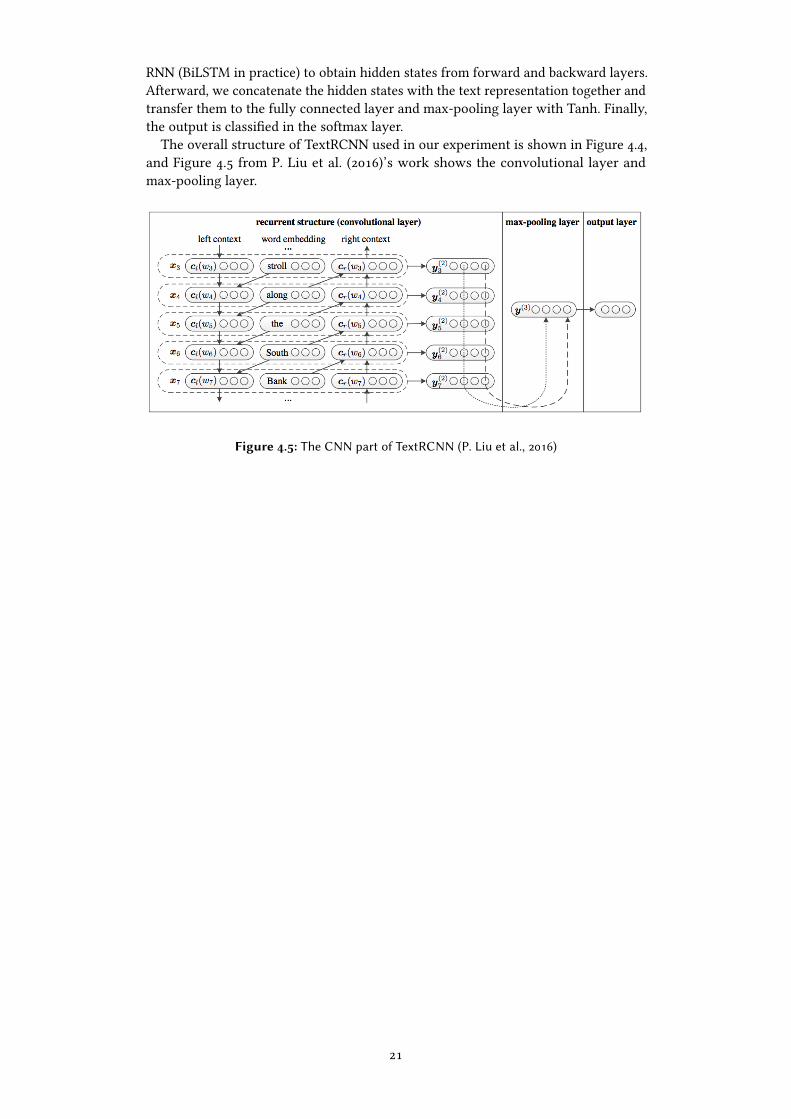
RNN (BiLSTM in practice) to obtain hidden states from forward and backward layers.
Afterward, we concatenate the hidden states with the text representation together and
transfer them to the fully connected layer and max-pooling layer with Tanh. Finally,
the output is classi�ed in the softmax layer.
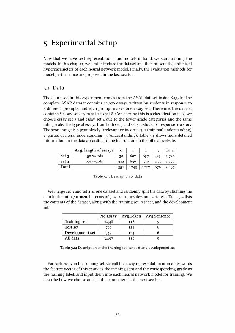
The overall structure of TextRCNN used in our experiment is shown in Figure 4.4,
and Figure 4.5 from P. Liu et al. (2016)’s work shows the convolutional layer and
max-pooling layer.
Figure 4.5: The CNN part of TextRCNN (P. Liu et al., 2016)
21
5 Experimental Setup
Now that we have text representations and models in hand, we start training the
models. In this chapter, we �rst introduce the dataset and then present the optimized
hyperparameters of each neural network model. Finally, the evaluation methods for
model performance are proposed in the last section.
5.1 Data
The data used in this experiment comes from the ASAP dataset inside Kaggle. The
complete ASAP dataset contains 12,976 essays written by students in response to
8 di�erent prompts, and each prompt makes one essay set. Therefore, the dataset
contains 8 essay sets from set 1 to set 8. Considering this is a classi�cation task, we
choose essay set 3 and essay set 4 due to the fewer grade categories and the same
rating scale. The type of essays from both set 3 and set 4 is students’ response to a story.
The score range is 0 (completely irrelevant or incorrect), 1 (minimal understanding),
2 (partial or literal understanding), 3 (understanding). Table 5.1 shows more detailed
information on the data according to the instruction on the o�cial website.
Avg. length of essays 0 1 2 3 Total
Set 3 150 words 39 607 657 423 1,726
Set 4 150 words 312 636 570 253 1,771
Total 351 1243 1227 676 3,497
Table 5.1: Description of data
We merge set 3 and set 4 as one dataset and randomly split the data by shu�ing the
data in the ratio 70:10:20, in terms of 70% train, 10% dev, and 20% test. Table 5.2 lists
the contents of the dataset, along with the training set, test set, and the development
set.
No.Essay Avg.Token Avg.SentenceTraining set 2,448 118 5
Test set 700 121 6
Development set 349 124 6
All data 3,497 119 5
Table 5.2: Description of the training set, text set and development set
For each essay in the training set, we call the essay representation or in other words
the feature vector of this essay as the training sent and the corresponding grade as
the training label, and input them into each neural network model for training. We
describe how we choose and set the parameters in the next section.
22
5.2 Hyperparameter Se�ings
Hyperparameters are the variables that determine the network structure and how
the network is trained. Some examples of hyperparameters in machine learning in-
clude Learning Rate, Number of Epochs, k-means, etc. Since hyperparameters can
have a direct impact on the model training, it is important to optimize them for best
performance.
Actually, it is not an easy task to con�gure neural networks, and there are many
parameters that need to be set. We grid search a set of manually prede�ned hyperpa-
rameters and use the value of the best performing hyperparameter. Those prede�ned
hyperparameters are selected from default values and some typical choices used in
other research studies. We tune the following hyperparameters. The �rst three hyper-
parameters are related to the training algorithm.
• Batch Size: Batch size refers to the number of samples selected for one training.
The size of the batch a�ects the optimization and speed of the model. A too large
batch size usually leads to poor generalization of features, while using a too
small batch size may have faster convergence to "good" results but the results
may not be global optima.
• Learning Rate: The learning rate determines whether the objective function
can converge to the local minimum and when it converges to the minimum. If
the learning rate is set too low, the training progress will be very slow due to
small updates to the weights. On the contrary, if the learning rate is set too high,
an undesirable divergence behavior may happen in the loss function. Therefore,
a decaying Learning rate is usually preferred.
• Number of Epochs: One epoch refers to one pass of the entire training data
through the neural network. An epoch consists of one or more batches. Tradi-
tionally, the number of epochs is very large, usually hundreds or thousands of
them, which allows the learning algorithm to keep running until the error from
the model is su�ciently minimized.
The rest of the hyperparameters are associated with network structure.
• Optimization and Loss Function: In most learning networks, the error is calcu-
lated as the di�erence between the actual output and the predicted output. The
loss function is used to compute such error. The current error usually propagates
backward to the previous layer, where the weights and biases are modi�ed to
minimize the error, then an optimization function is needed.
• Activation Function: The activation function introduces nonlinearity to models.
It is used to convert the activation level of a neuron into an output signal (Karlik
and Olgac, 2011). Without the activation function, the output of each layer of
the neural network is a linear function of the upper layer input. In that case, the
neural network is not of practical signi�cance anymore.
• Hidden Layers and Neurons: Hidden layers refer to the layers between the
input layer and the output layer. There may be one or more layers. The hidden
layer does not receive nor send signals directly. The neurons in each hidden
layer calculate the weighted sum of inputs and weights, add the bias and execute
an activation function. The number of neurons in each layer is usually termed
layer size.
23

• Dropout Rate: Dropout is a regularization technique that can avoid over�tting
and improve generalization ability via randomly omitting half of the feature
detectors on each batch. The probability of neuron cancellation is the dropout
rate.
The hyperparameter settings of the three neural network models are roughly the
same. The speci�c hyperparameters and values for the neural network models are
listed in Table 5.3.
TextCNN
TextRNN_LSTM
TextRNN_GRU
TextRCNN
Bidirectional - True True
Activation function ReLU Tanh Tanh
Optimization Adam Adam Adam
Loss function Cross Entropy Loss Cross Entropy Loss Cross Entropy Loss
Learning rate 0.0001 0.0001 0.0001
Batch size 64 32 32
Dropout rate 0.2 0.2 0.2
Number of layers - 2 2
Hidden size 300 300 300
Number of epochs 1000 200 200
Number of Filters 128 - -
Filter size [1,2,3,4,5] - -
Table 5.3: Hyperparameters for neural network models
The activation function is the same as the initial setting. Moreover, for TextCNN,
we set the �lter size = (h = [1,2,3,4,5]) on the basis of Kim (2014)’s work, and the �lter
channel is set to 128. The above hyper-parameters are tuned on the validation set, and
early stopping is used with the number of epochs.
5.3 Evaluation Matrix
In order to evaluate the model performance, we resort to three measurements: Accuracy,
F1 score, and the Quadratic weighted Kappa (QWK).
Accuracy is the measure of all the correctly identi�ed cases. However, it may cause
a misleading performance measure for highly imbalanced data because it provides an
over-optimistic estimation of the classi�er ability on the majority class (Chicco and
Jurman, 2020). Therefore, Accuracy alone is not enough to evaluate model performance.
F-score or F-measure is an e�ective solution to overcome data imbalance. It is a
weighted average of the precision and recall, where the precision is the ratio between
the number of essays correctly predicted as i and the number of essays predicted as i,including those not identi�ed correctly, and the recall is the number of essays correctly
predicted as i divided by the number of essays assigned with i by human raters.
In our experiment, we exploit the F1 score which is the harmonic mean of precision
and recall and it penalizes extreme values:
F1 score = 2 × %A428B8>= × '420;;%A428B8>= + '420;; (5.1)
QWK is a popular metric in Kaggle competitions, and a standard instrument to
measure the accuracy of all multi-value classi�cation problems. It is derived from
24
Cohen’s Kappa statistic (Ben-David, 2008). Kappa or Cohen’s Kappa can basically tell
us how much better the neural network is performing over the performance of the
model that simply guesses at random. Thus, it compensates for classi�cations that
may have been accidental.
According to the calculation method of kappa, it is divided into simple kappa and
weighted kappa. Weighted kappa is further divided into linear weighted kappa and
quadratic weighted kappa. The QWK typically ranges from 0 to 1. The higher the
QWK value, the better performance of the models. The value can even go below zero
if there is less agreement between two outcomes than expected by chance. In general,
it will be regarded as an ideal degree of agreement when the QWK value is greater
than 0.75.
In order to calculate the QWK value, we �rst need a weighted matrix. The formula
is as follows,
,8, 9 =(8 − 9)2(# − 1)2 (5.2)
W is an N*N matrix, with i representing the actual score assigned by human raters,
and j referring to the predicted score. N is the total number of categories. For example,
the rating scale of our data is 0-3, so N equals 4.
= 1 −∑8, 9,8, 9$8, 9∑8, 9,8, 9�8, 9
(5.3)
The observed matrix $8, 9 and the expected matrix �8, 9 are both N-by-N histogram
matrices. $8, 9 corresponds to the number of essays that are assigned with score i by
human raters but predicted as j (j may or may not be the same to i). �8, 9 is calculated
as the outer product between the actual scores and the predicted scores. We explain it
with a speci�c example. The number of essays in the training set is 2,448. Suppose
700 essays in the training set are manually scored as 1 point. Of these 700 essays, 200
are predicted by the model to be 0 points. At the same time, there are a total of 400
essays predicted by the model to be 0 points in the training set. Then $1,0 is 200, and
�1,0 should be 700 ×400/2, 448≈114. Finally, the QWK can be worked out from these
three matrices.
25
6 Results and Analysis
In this chapter, we give an exhibition of the experimental results with evaluation
metrics in terms of Accuracy, F1 score, and QWK. The sections in this chapter are
ordered according to the research questions proposed in Chapter 1.
6.1 Research �estion 1
Question 1: What results could be achieved for automatic essay scoring for English,
using similar linguistic features as have previously been used for Swedish?
First of all, the baseline models are chosen from variants of SVM, which are Lin-
earSVR and LinearSVC. The parameters are set with the default value. Table 6.1 shows a
comparison between these SVMs and neural network models in the aspect of accuracy,
F1, and QWK.
Accuracy F1 Score QWKLinearSVR 52.36% 0.53 0.48
LinearSVC 47.35% 0.46 0.56
TextCNN 42.49% 0.43 0.36
TextRNN_LSTM 54.79% 0.55 0.59TextRNN_GRU 54.08% 0.5 0.52
TextRCNN 42.78% 0.41 0.37
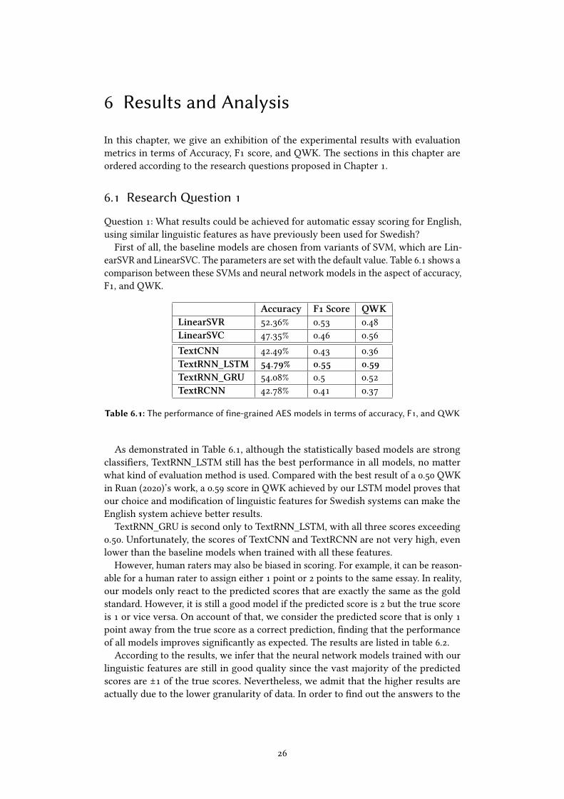
Table 6.1: The performance of fine-grained AES models in terms of accuracy, F1, and QWK
As demonstrated in Table 6.1, although the statistically based models are strong
classi�ers, TextRNN_LSTM still has the best performance in all models, no matter
what kind of evaluation method is used. Compared with the best result of a 0.50 QWK
in Ruan (2020)’s work, a 0.59 score in QWK achieved by our LSTM model proves that
our choice and modi�cation of linguistic features for Swedish systems can make the
English system achieve better results.
TextRNN_GRU is second only to TextRNN_LSTM, with all three scores exceeding
0.50. Unfortunately, the scores of TextCNN and TextRCNN are not very high, even
lower than the baseline models when trained with all these features.
However, human raters may also be biased in scoring. For example, it can be reason-
able for a human rater to assign either 1 point or 2 points to the same essay. In reality,
our models only react to the predicted scores that are exactly the same as the gold
standard. However, it is still a good model if the predicted score is 2 but the true score
is 1 or vice versa. On account of that, we consider the predicted score that is only 1
point away from the true score as a correct prediction, �nding that the performance
of all models improves signi�cantly as expected. The results are listed in table 6.2.
According to the results, we infer that the neural network models trained with our
linguistic features are still in good quality since the vast majority of the predicted
scores are ±1 of the true scores. Nevertheless, we admit that the higher results are
actually due to the lower granularity of data. In order to �nd out the answers to the
26
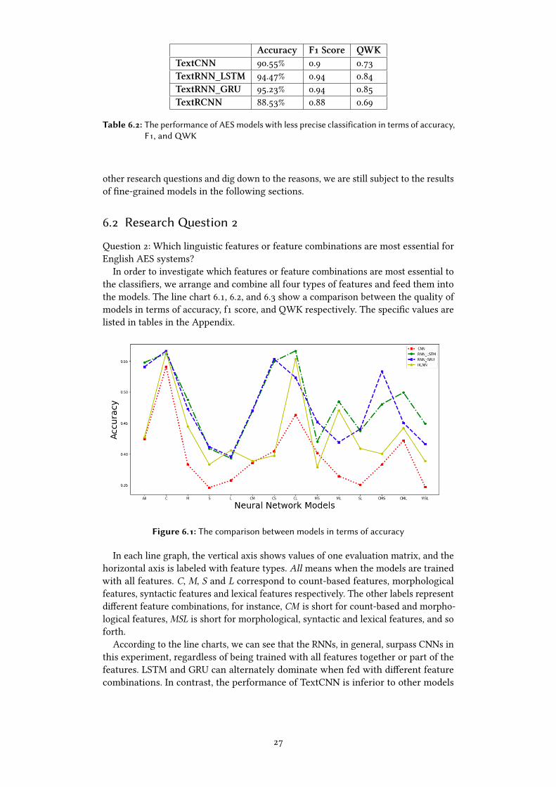
Accuracy F1 Score QWKTextCNN 90.55% 0.9 0.73
TextRNN_LSTM 94.47% 0.94 0.84
TextRNN_GRU 95.23% 0.94 0.85
TextRCNN 88.53% 0.88 0.69
Table 6.2: The performance of AES models with less precise classification in terms of accuracy,
F1, and QWK
other research questions and dig down to the reasons, we are still subject to the results
of �ne-grained models in the following sections.
6.2 Research �estion 2
Question 2: Which linguistic features or feature combinations are most essential for
English AES systems?
In order to investigate which features or feature combinations are most essential to
the classi�ers, we arrange and combine all four types of features and feed them into
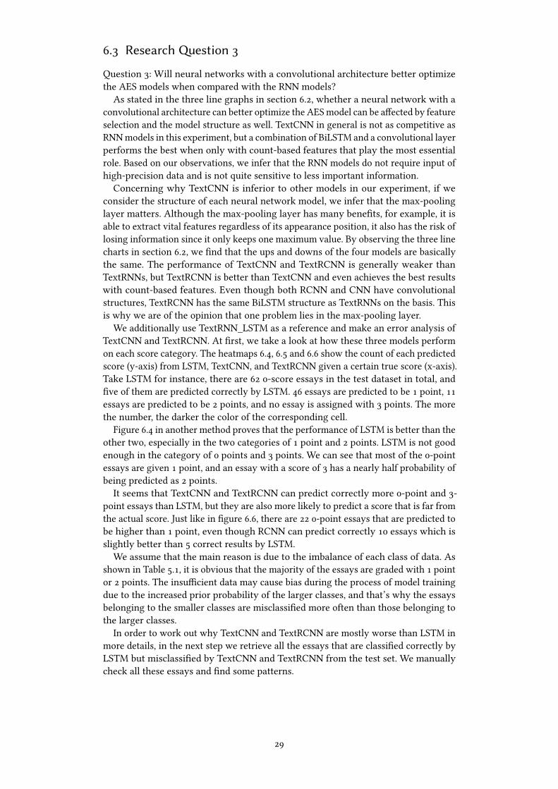
the models. The line chart 6.1, 6.2, and 6.3 show a comparison between the quality of
models in terms of accuracy, f1 score, and QWK respectively. The speci�c values are
listed in tables in the Appendix.
Figure 6.1: The comparison between models in terms of accuracy
In each line graph, the vertical axis shows values of one evaluation matrix, and the
horizontal axis is labeled with feature types. All means when the models are trained
with all features. C, M, S and L correspond to count-based features, morphological
features, syntactic features and lexical features respectively. The other labels represent
di�erent feature combinations, for instance, CM is short for count-based and morpho-
logical features, MSL is short for morphological, syntactic and lexical features, and so
forth.
According to the line charts, we can see that the RNNs, in general, surpass CNNs in
this experiment, regardless of being trained with all features together or part of the
features. LSTM and GRU can alternately dominate when fed with di�erent feature
combinations. In contrast, the performance of TextCNN is inferior to other models
27
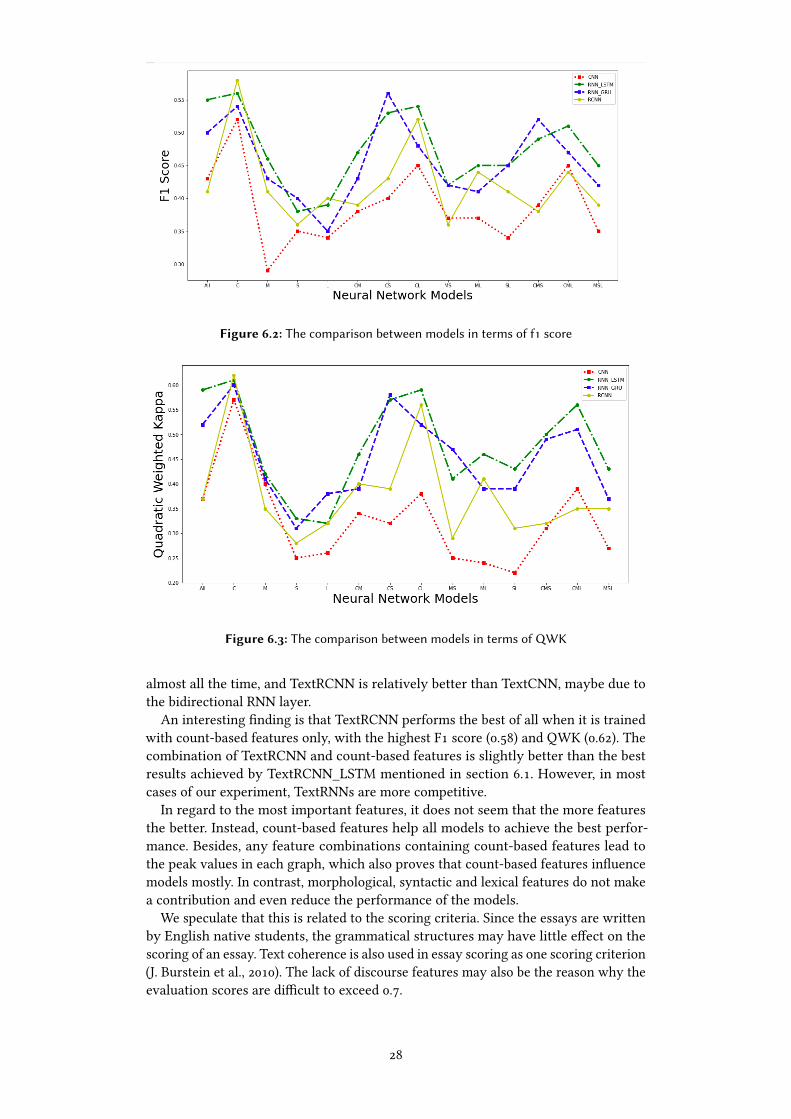
Figure 6.2: The comparison between models in terms of f1 score
Figure 6.3: The comparison between models in terms of QWK
almost all the time, and TextRCNN is relatively better than TextCNN, maybe due to
the bidirectional RNN layer.
An interesting �nding is that TextRCNN performs the best of all when it is trained
with count-based features only, with the highest F1 score (0.58) and QWK (0.62). The
combination of TextRCNN and count-based features is slightly better than the best
results achieved by TextRCNN_LSTM mentioned in section 6.1. However, in most
cases of our experiment, TextRNNs are more competitive.
In regard to the most important features, it does not seem that the more features
the better. Instead, count-based features help all models to achieve the best perfor-
mance. Besides, any feature combinations containing count-based features lead to
the peak values in each graph, which also proves that count-based features in�uence
models mostly. In contrast, morphological, syntactic and lexical features do not make
a contribution and even reduce the performance of the models.
We speculate that this is related to the scoring criteria. Since the essays are written
by English native students, the grammatical structures may have little e�ect on the
scoring of an essay. Text coherence is also used in essay scoring as one scoring criterion
(J. Burstein et al., 2010). The lack of discourse features may also be the reason why the
evaluation scores are di�cult to exceed 0.7.
28
6.3 Research �estion 3
Question 3: Will neural networks with a convolutional architecture better optimize
the AES models when compared with the RNN models?
As stated in the three line graphs in section 6.2, whether a neural network with a
convolutional architecture can better optimize the AES model can be a�ected by feature
selection and the model structure as well. TextCNN in general is not as competitive as
RNN models in this experiment, but a combination of BiLSTM and a convolutional layer
performs the best when only with count-based features that play the most essential
role. Based on our observations, we infer that the RNN models do not require input of
high-precision data and is not quite sensitive to less important information.
Concerning why TextCNN is inferior to other models in our experiment, if we
consider the structure of each neural network model, we infer that the max-pooling
layer matters. Although the max-pooling layer has many bene�ts, for example, it is
able to extract vital features regardless of its appearance position, it also has the risk of
losing information since it only keeps one maximum value. By observing the three line
charts in section 6.2, we �nd that the ups and downs of the four models are basically
the same. The performance of TextCNN and TextRCNN is generally weaker than
TextRNNs, but TextRCNN is better than TextCNN and even achieves the best results
with count-based features. Even though both RCNN and CNN have convolutional
structures, TextRCNN has the same BiLSTM structure as TextRNNs on the basis. This
is why we are of the opinion that one problem lies in the max-pooling layer.
We additionally use TextRNN_LSTM as a reference and make an error analysis of
TextCNN and TextRCNN. At �rst, we take a look at how these three models perform
on each score category. The heatmaps 6.4, 6.5 and 6.6 show the count of each predicted
score (y-axis) from LSTM, TextCNN, and TextRCNN given a certain true score (x-axis).
Take LSTM for instance, there are 62 0-score essays in the test dataset in total, and
�ve of them are predicted correctly by LSTM. 46 essays are predicted to be 1 point, 11
essays are predicted to be 2 points, and no essay is assigned with 3 points. The more
the number, the darker the color of the corresponding cell.
Figure 6.4 in another method proves that the performance of LSTM is better than the
other two, especially in the two categories of 1 point and 2 points. LSTM is not good
enough in the category of 0 points and 3 points. We can see that most of the 0-point
essays are given 1 point, and an essay with a score of 3 has a nearly half probability of
being predicted as 2 points.
It seems that TextCNN and TextRCNN can predict correctly more 0-point and 3-
point essays than LSTM, but they are also more likely to predict a score that is far from
the actual score. Just like in �gure 6.6, there are 22 0-point essays that are predicted to
be higher than 1 point, even though RCNN can predict correctly 10 essays which is
slightly better than 5 correct results by LSTM.
We assume that the main reason is due to the imbalance of each class of data. As
shown in Table 5.1, it is obvious that the majority of the essays are graded with 1 point
or 2 points. The insu�cient data may cause bias during the process of model training
due to the increased prior probability of the larger classes, and that’s why the essays
belonging to the smaller classes are misclassi�ed more often than those belonging to
the larger classes.
In order to work out why TextCNN and TextRCNN are mostly worse than LSTM in
more details, in the next step we retrieve all the essays that are classi�ed correctly by
LSTM but misclassi�ed by TextCNN and TextRCNN from the test set. We manually
check all these essays and �nd some patterns.
29

Figure 6.4: LSTM
Figure 6.5: TextCNN
We �rst analyze the errors of TextCNN. After comparison, we �nd that CNN is
inferior to LSTM for processing long sentences, especially when dealing with depen-
dent clauses. Table 6.3 lists three essay examples of this point with dependent clauses
underlined.
We indicate that the predictions of TextCNN and TextRNN_LSTM do not di�er
greatly when there are fewer dependent clauses. We only �nd one clause in the �rst
30

Figure 6.6: TextRCNN
essay example, and the di�erence between the prediction result of TextCNN and the
correct result is only 1 point. Nevertheless, if there are more than a couple of dependent
clauses like in the second and third essay examples, there will be a decrease in the
performance of TextCNN.
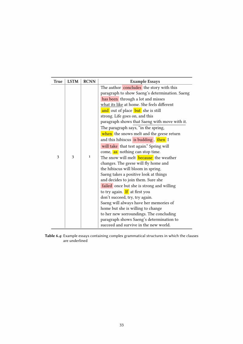
Besides TextCNN, the comparison between TextRNN_LSTM and TextRCNN seems
to have the same problem in long and complicated sentences as is shown in Figure
6.4. The conjunctions including both coordinating conjunctions and subordinating
conjunctions are marked with yellow, and the dependent clauses are underlined. We
also mark di�erent verb forms in pink.
We further try to use TextRCNN as a reference and perform error analysis on
TextCNN. As they use di�erent methods to obtain features, and overall TextRCNN
performs better than TextCNN to some degree, we infer that the recurrent structure is
indeed more suitable for our experiments. However, because our sample is not large
enough, the comparison of the data samples is not su�cient for us to speculate about
what patterns the recurrent layer and convolutional layer have learned. We hope that
we can make up this point by adding more data in the future.
31

True LSTM CNN Example Essays
2 2 3
When the cyclist began his journey he was
con�dent in succeeding. Throughout the story however,
the cyclist endures many con�icts to his successs
in his journey. The cyclist faced his �rst
di��culty once he reached a small, abandoned town.
“I had been hitting my water bottles pretty regularly,
and I was traveling through the high deserts of
California in June” (kurmaskie @NUM1). The cyclist
realized he had not conserved his water and his
“water bottles contained only a few tantalizing sips”
(kurmaskie @NUM1). On top of his water problem
the heat was unbelievable. He was losing
hydration from all the sweat, and he was
losing it quickly. The cyclist was also
dealing with the di�cult roads. There were
many things this cyclist endured through-out his
journey, but he was determined to �nish his
trip and was �lled with satisfaction once
he overcame these hardships.
3 3 1
I think the author is just trying to show that
you never give up. I think the author is
trying to show the beautie of nature. The author
used that because in the story Saeng failed the test
but at the end it says that she will take
the test again. In the story it talks about
the winter hibiscus that she planted and that is
concluded in the conclusion. The conclusion basiclly
saying is there will be a new beginning.
2 2 0
The author concludes the last paragraph to show
that after a time period you can come back
and try something again. Or maybe when weather
change this can be di�erent for Saeng.
Maybe she is relating herself to the plant as to
when it come to spring
the �ower will be stronger, and she feel
that she will pass the test second time around
when the geese come back and the hibiscus is budding.
And it also shows how she appriate the nature
because if not, why would she wait until spring
and when the snow is melting.
The conclusion of the story is
that she do like nature,
because she talk about the hibiscus.
Table 6.3: Example essays containing complex grammatical structures in which the clauses
are underlined. LSTM in here is short for TextRNN_LSTM and CNN is short for
TextCNN.
32
True LSTM RCNN Example Essays
3 3 1
The author concludes the story with this
paragraph to show Saeng’s determination. Saeng
has been through a lot and misses
what its like at home. She feels di�erent
and out of place but she is still
strong. Life goes on, and this
paragraph shows that Saeng with move with it.
The paragraph says, “in the spring,
when the snows melt and the geese return
and this hibiscus is budding , then I
will take that test again.” Spring will
come, as nothing can stop time.
The snow will melt because the weather
changes. The geese will �y home and
the hibiscus will bloom in spring.
Saeng takes a positive look at things
and decides to join them. Sure she
failed once but she is strong and willing
to try again. If at �rst you
don’t succeed, try, try again.
Saeng will always have her memories of
home but she is willing to change
to her new sorroundings. The concluding
paragraph shows Saeng’s determination to
succeed and survive in the new world.
Table 6.4: Example essays containing complex grammatical structures in which the clauses
are underlined
33
7 Conclusion
This thesis work attempts to explore the automated essay scoring (AES) for English
based on neural network models trained on arti�cially extracted linguistic features.
The neural network models include TextCNN, TextRNN_LSTM, TextRNN_GRU, and
TextRCNN. We extract the linguistic features of the essays from the ASAP dataset.
The features cover four aspects based on frequencies, morphology, syntax, and lexis.
We mainly answer three questions in this work. First, if existing linguistic features
extracted for another European language, which is Swedish in this thesis work, can
also play a role in automated English essay scoring? Second, which linguistic features
or feature combinations contribute the most to the performance of the models? Finally,
compared with each other, how do the four neural network models perform?
For the �rst question, our results show that the best performance is achieved by
TextRNN_LSTM when trained with all features, with an accuracy of 54.79%, an F1 score
of 0.55, and a quadratic weighted kappa (QWK) of 0.59, followed by TextRNN_GRU.
The TextRNN models successfully beat the statistical baseline models, and even get
a higher QWK score than their Swedish counterparts, which means that the feature
selection for Swedish AES systems can be used as a good reference for English systems.
It is also worth noting that even if our model predicts incorrectly, the di�erence
between the wrong score and the real score is only 1 point in most cases.
With respect to the second question, we examine models trained on not only a
single feature type, but also on 9 other feature combinations. Our experimental results
show that count-based features are most helpful to improve the performance of the
model, while other features are more or less counterproductive. However, while we
were trying to �nd the answers to the second question, we happened to �nd that
TextRCNN with count-based features achieved the best results of all experimental
results, with 2 out of 3 evaluation metrics (F1 score: 0.58, QWK: 0.62) superior to other
models. Regarding the third question, a combination of BiLSTM and a convolutional
structure can optimize the AES system for English but only with high-precision input
data. On the contrary, when it is uncertain what linguistic features to choose, TextRNN
models are more likely to provide accurate classi�cation. We suspect that it is due to
the max-pooling layer that may lose some information of features. According to our
observation, the missing information can be about syntactic features. For example,
when there are more grammatically complex sentences in an essay, the performance of
the convolutional network is not as good as the recurrent network. Another reason is
the lack of data, resulting in the CNN models not being able to learn linguistic features
well.
Due to time constraints, there are some �aws in our experiment. In future related
experiments, we will mainly make up for these shortcomings from the following points.
First of all, if we still use the same database, we will consider adding discourse features,
and then only keep count-based features to see if the performance of the model can be
further improved. Or we still keep all four features together with discourse features
and then see if there are new discoveries. Secondly, we also want to try more updated
models, such as transformer or BERT to see if their classi�cation e�ect will surpass
TextRNN_LSTM. Another point is that we can enlarge the dataset, or we choose other
languages in the universal dependencies to see if the AES system can be universally
34

used in other languages, such as Mandarin and Japanese which is quite di�erent from
Indo-European languages.
35
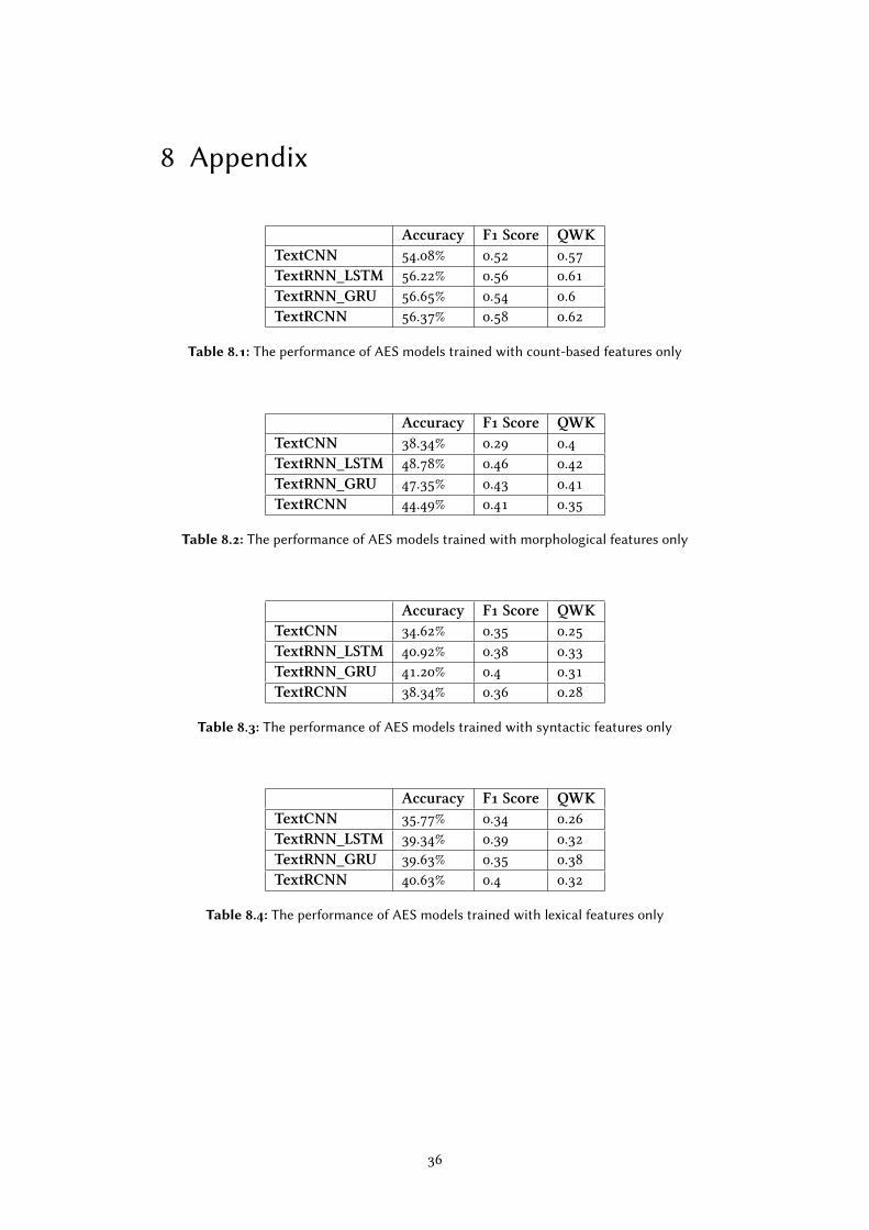
8 Appendix
Accuracy F1 Score QWKTextCNN 54.08% 0.52 0.57
TextRNN_LSTM 56.22% 0.56 0.61
TextRNN_GRU 56.65% 0.54 0.6
TextRCNN 56.37% 0.58 0.62
Table 8.1: The performance of AES models trained with count-based features only
Accuracy F1 Score QWKTextCNN 38.34% 0.29 0.4
TextRNN_LSTM 48.78% 0.46 0.42
TextRNN_GRU 47.35% 0.43 0.41
TextRCNN 44.49% 0.41 0.35
Table 8.2: The performance of AES models trained with morphological features only
Accuracy F1 Score QWKTextCNN 34.62% 0.35 0.25
TextRNN_LSTM 40.92% 0.38 0.33
TextRNN_GRU 41.20% 0.4 0.31
TextRCNN 38.34% 0.36 0.28
Table 8.3: The performance of AES models trained with syntactic features only
Accuracy F1 Score QWKTextCNN 35.77% 0.34 0.26
TextRNN_LSTM 39.34% 0.39 0.32
TextRNN_GRU 39.63% 0.35 0.38
TextRCNN 40.63% 0.4 0.32
Table 8.4: The performance of AES models trained with lexical features only
36

Accuracy F1 Score QWKTextCNN 38.63% 0.38 0.34
TextRNN_LSTM 46.92% 0.47 0.46
TextRNN_GRU 47.07% 0.43 0.39
TextRCNN 38.91% 0.39 0.4
Table 8.5: The performance of AES models trained with count and morphological features
Accuracy F1 Score QWKTextCNN 40.49% 0.4 0.32
TextRNN_LSTM 54.94% 0.53 0.57
TextRNN_GRU 55.36% 0.56 0.58
TextRCNN 39.77% 0.43 0.39
Table 8.6: The performance of AES models trained with count and syntactic features
Accuracy F1 Score QWKTextCNN 46.35% 0.45 0.38
TextRNN_LSTM 56.65% 0.54 0.59
TextRNN_GRU 52.36% 0.48 0.52
TextRCNN 55.36% 0.52 0.56
Table 8.7: The performance of AES models trained with count and lexical features
Accuracy F1 Score QWKTextCNN 40.20% 0.37 0.25
TextRNN_LSTM 42.06% 0.42 0.41
TextRNN_GRU 45.21% 0.42 0.47
TextRCNN 37.91% 0.36 0.29
Table 8.8: The performance of AES models trained with morphological and syntactical fea-
tures
Accuracy F1 Score QWKTextCNN 36.48% 0.37 0.24
TextRNN_LSTM 48.50% 0.45 0.46
TextRNN_GRU 41.92% 0.41 0.39
TextRCNN 47.07% 0.44 0.41
Table 8.9: The performance of AES models trained with morphological and lexical features
Accuracy F1 Score QWKTextCNN 35.05% 0.34 0.22
TextRNN_LSTM 43.78% 0.45 0.43
TextRNN_GRU 44.06% 0.45 0.39
TextRCNN 40.92% 0.41 0.31
Table 8.10: The performance of AES models trained with syntactical and lexical features
37
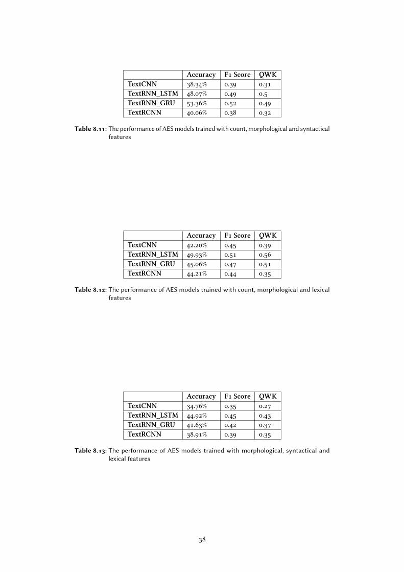
Accuracy F1 Score QWKTextCNN 38.34% 0.39 0.31
TextRNN_LSTM 48.07% 0.49 0.5
TextRNN_GRU 53.36% 0.52 0.49
TextRCNN 40.06% 0.38 0.32
Table 8.11: The performance of AES models trained with count, morphological and syntactical
features
Accuracy F1 Score QWKTextCNN 42.20% 0.45 0.39
TextRNN_LSTM 49.93% 0.51 0.56
TextRNN_GRU 45.06% 0.47 0.51
TextRCNN 44.21% 0.44 0.35
Table 8.12: The performance of AES models trained with count, morphological and lexical
features
Accuracy F1 Score QWKTextCNN 34.76% 0.35 0.27
TextRNN_LSTM 44.92% 0.45 0.43
TextRNN_GRU 41.63% 0.42 0.37
TextRCNN 38.91% 0.39 0.35
Table 8.13: The performance of AES models trained with morphological, syntactical and
lexical features
38
Bibliography
Aggarwal, Mukul (2011). “Information retrieval and question answering nlp approach:
an arti�cial intelligence application”. International Journal of Soft Computing andEngineering (IJSCE) 1.NCAI2011.
Alikaniotis, Dimitrios, Helen Yannakoudakis, and Marek Rei (2016). “Automatic text
scoring using neural networks”. arXiv preprint arXiv:1606.04289.
Ben-David, Arie (2008). “Comparison of classi�cation accuracy using Cohen’s Weighted
Kappa”. Expert Systems with Applications 34.2, pp. 825–832.
Biber, Douglas and Edward Finegan (2008). “Longman: grammar of spoken and written
english”. In: Longman: grammar of spoken and written english, pp. 1204–1204.
Breland, Hunter M, Robert J Jones, Laura Jenkins, Marion Paynter, Judith Pollack, and
Y Fai Fong (1994). “The college board vocabulary study”. ETS Research Report Series1994.1, pp. i–51.
Burstein, Jill, Karen Kukich, Susanne Wol�, Chi Lu, and Martin Chodorow (2001).
“Enriching Automated Essay Scoring Using Discourse Marking.”
Burstein, Jill, Joel Tetreault, and Slava Andreyev (2010). “Using entity-based features
to model coherence in student essays”. In: Human language technologies: The 2010annual conference of the North American chapter of the Association for ComputationalLinguistics, pp. 681–684.
Cai, Jingjing, Jianping Li, Wei Li, and Ji Wang (2018). “Deeplearning model used in text
classi�cation”. In: 2018 15th International Computer Conference on Wavelet ActiveMedia Technology and Information Processing (ICCWAMTIP). IEEE, pp. 123–126.
Chen, Hongbo and Ben He (2013). “Automated essay scoring by maximizing human-
machine agreement”. In: Proceedings of the 2013 Conference on Empirical Methods inNatural Language Processing, pp. 1741–1752.
Chen, Zhiyun and Yuxin Zhou (2019). “Research on automatic essay scoring of com-
position based on CNN and OR”. In: 2019 2nd International Conference on Arti�cialIntelligence and Big Data (ICAIBD). IEEE, pp. 13–18.
Chicco, Davide and Giuseppe Jurman (2020). “The advantages of the Matthews correla-
tion coe�cient (MCC) over F1 score and accuracy in binary classi�cation evaluation”.
BMC genomics 21.1, pp. 1–13.
Collobert, Ronan, Jason Weston, Léon Bottou, Michael Karlen, Koray Kavukcuoglu, and
Pavel Kuksa (2011). “Natural language processing (almost) from scratch”. Journal ofmachine learning research 12.ARTICLE, pp. 2493–2537.
Cozma, Mădălina, Andrei M Butnaru, and Radu Tudor Ionescu (2018). “Automated essay
scoring with string kernels and word embeddings”. arXiv preprint arXiv:1804.07954.
Crossley, Scott A, Kristopher Kyle, and Danielle S McNamara (2015). “To Aggregate
or Not? Linguistic Features in Automatic Essay Scoring and Feedback Systems.”
Grantee Submission 8.1.
Crowston, Kevin, Xiaozhong Liu, and Eileen E Allen (2010). “Machine learning and
rule-based automated coding of qualitative data”. proceedings of the American Societyfor Information Science and Technology 47.1, pp. 1–2.
Dasgupta, Tirthankar, Abir Naskar, Lipika Dey, and Rupsa Saha (2018). “Augment-
ing textual qualitative features in deep convolution recurrent neural network for
automatic essay scoring”. In: Proceedings of the 5th Workshop on Natural LanguageProcessing Techniques for Educational Applications, pp. 93–102.
39
Dikli, Semire (2006). “Automated essay scoring”. Turkish Online Journal of DistanceEducation 7.1, pp. 49–62.
Dong, Fei, Yue Zhang, and Jie Yang (2017). “Attention-based recurrent convolutional
neural network for automatic essay scoring”. In: Proceedings of the 21st conferenceon computational natural language learning (CoNLL 2017), pp. 153–162.
Elliot, S and C Mikulas (2004). “How does IntelliMetric TM score essay responses?
A mind based approach”. In: annual meeting of the American Educational ResearchAssociation, San Diego, CA.
Falkenjack, Johan, Katarina Heimann Mühlenbock, and Arne Jönsson (2013). “Features
indicating readability in Swedish text”. In: Proceedings of the 19th Nordic Conferenceof Computational Linguistics (NODALIDA 2013), pp. 27–40.
Fišer, Darja and Jakob Lenardič (2019). “Overview of tools for text normalization”.
Ghanta, Harshanthi (2019). “Automated Essay Evaluation Using Natural Language
Processing and Machine Learning”.
Hearst, Marti A (2000). “The debate on automated essay grading”. IEEE IntelligentSystems and their Applications 15.5, pp. 22–37.
Karlik, Bekir and A Vehbi Olgac (2011). “Performance analysis of various activation
functions in generalized MLP architectures of neural networks”. International Journalof Arti�cial Intelligence and Expert Systems 1.4, pp. 111–122.
Ke, Zixuan and Vincent Ng (2019). “Automated Essay Scoring: A Survey of the State
of the Art.” In: IJCAI. Vol. 19, pp. 6300–6308.
Kilgarri�, Adam, Frieda Charalabopoulou, Maria Gavrilidou, Janne Bondi Johannessen,
Saussan Khalil, So�e Johansson Kokkinakis, Robert Lew, Serge Sharo�, Ravikiran
Vadlapudi, and Elena Volodina (2014). “Corpus-based vocabulary lists for language
learners for nine languages”. Language resources and evaluation 48.1, pp. 121–163.
Kim, Yoon (2014). “Convolutional neural networks for sentence classi�cation”. url:
https://arxiv.org/pdf/1408.5882.pdf.
Klebanov, Beata Beigman, Michael Flor, and Binod Gyawali (2016). “Topicality-based
indices for essay scoring”. In: Proceedings of the 11th Workshop on Innovative Use ofNLP for Building Educational Applications, pp. 63–72.
Lai, Siwei, Liheng Xu, Kang Liu, and Jun Zhao (2015). “Recurrent convolutional neural
networks for text classi�cation”. In: Twenty-ninth AAAI conference on arti�cialintelligence. url: http://zhengyima.com/my/pdfs/Textrcnn.pdf.
Landauer, Thomas K and W Kintsch (2003). “Latent semantic analysis”. AutomatedEssay Scoring: A Cross-disciplinary Perspective, p. 87.
Linden, Anné and Kathrin Perutz (2008). Mindworks: An introduction to NLP. Crown
House Publishing.
Liu, Jiawei, Yang Xu, and Yaguang Zhu (2019). “Automated essay scoring based on
two-stage learning”. arXiv preprint arXiv:1901.07744. url: https://ui.adsabs.harvard.
edu/abs/2019arXiv190107744L/abstract.
Liu, Pengfei, Xipeng Qiu, and Xuanjing Huang (2016). “Recurrent neural network for
text classi�cation with multi-task learning”. arXiv preprint arXiv:1605.05101.
Madnani, Nitin and Aoife Cahill (2018). “Automated scoring: Beyond natural language
processing”. In: Proceedings of the 27th International Conference on ComputationalLinguistics, pp. 1099–1109.
Mayo, Matthew (2017). “A general approach to preprocessing text data”. KDnuggets,https://www. kdnuggets. com/2017/12/general-approach-preprocessing-text-data. html.
Meurers, Detmar (2012). “Natural language processing and language learning”. Ency-clopedia of applied linguistics, pp. 4193–4205.
Page, Ellis B (1966). “The imminence of... grading essays by computer”. The Phi DeltaKappan 47.5, pp. 238–243.
Page, Ellis Batten (2003). “Project Essay Grade: PEG.”
40

Persing, Isaac and Vincent Ng (2015). “Modeling argument strength in student essays”.
In: Proceedings of the 53rd Annual Meeting of the Association for ComputationalLinguistics and the 7th International Joint Conference on Natural Language Processing(Volume 1: Long Papers), pp. 543–552.
Phandi, Peter, Kian Ming A Chai, and Hwee Tou Ng (2015). “Flexible domain adaptation
for automated essay scoring using correlated linear regression”. In: Proceedings of the2015 Conference on Empirical Methods in Natural Language Processing, pp. 431–439.
Pilán, Ildikó (2018). Automatic pro�ciency level prediction for Intelligent Computer-Assisted Language Learning.
Rayner, Keith, Alexander Pollatsek, Jane Ashby, and Charles Clifton Jr (2012). “Psy-
chology of reading”.
Ruan, Rex Dajun (2020). Neural Network Based Atuomatic Essay Scoring for Swedish.
Rudner, Lawrence M, Veronica Garcia, and Catherine Welch (2006). “An evaluation
of IntelliMetric™ essay scoring system”. The Journal of Technology, Learning andAssessment 4.4.
Rudner, Lawrence M and Tahung Liang (2002). “Automated essay scoring using Bayes’
theorem”. The Journal of Technology, Learning and Assessment 1.2.
Shermis, Mark D and Jill C Burstein (2003).Automated essay scoring: A cross-disciplinaryperspective. Routledge.
Taghipour, Kaveh and Hwee Tou Ng (2016). “A neural approach to automated essay
scoring”. In: Proceedings of the 2016 conference on empirical methods in naturallanguage processing, pp. 1882–1891.
Tausczik, Yla R and James W Pennebaker (2010). “The psychological meaning of words:
LIWC and computerized text analysis methods”. Journal of language and socialpsychology 29.1, pp. 24–54.
Uto, Masaki and Masashi Okano (2020). “Robust neural automated essay scoring
using item response theory”. In: International Conference on Arti�cial Intelligence inEducation. Springer, pp. 549–561.
Vajjala, Sowmya (2018). “Automated assessment of non-native learner essays: Investi-
gating the role of linguistic features”. International Journal of Arti�cial Intelligencein Education 28.1, pp. 79–105.
Valenti, Salvatore, Francesca Neri, and Alessandro Cucchiarelli (2003). “An overview
of current research on automated essay grading”. Journal of Information TechnologyEducation: Research 2.1, pp. 319–330.
Walia, Tarandeep Singh, Gurpreet Singh Josan, and Amarpal Singh (2019). “An e�-
cient automated answer scoring system for Punjabi language”. Egyptian InformaticsJournal 20.2, pp. 89–96.
Wang, Jinhao and Michelle Stallone Brown (2007). “Automated essay scoring versus hu-
man scoring: A comparative study.” Journal of Technology, Learning, and Assessment6.2, n2.
Wang, Yucheng, Zhongyu Wei, Yaqian Zhou, and Xuan-Jing Huang (2018). “Automatic
essay scoring incorporating rating schema via reinforcement learning”. In: Pro-ceedings of the 2018 conference on empirical methods in natural language processing,
pp. 791–797.
Zhang, Mo (2013). “Contrasting automated and human scoring of essays”. R & DConnections 21.2, pp. 1–11.
Zhang, Ye and Byron Wallace (2015). “A sensitivity analysis of (and practitioners’
guide to) convolutional neural networks for sentence classi�cation”. arXiv preprintarXiv:1510.03820.
41