BMR JOURNAL OF AUSTRALIAN GEOLOGY & GEOPHYSICS VOLUME 1 57

Automated Density Profiling over elongate topographic features

W.Anfiloff

Nettleton's concept of density profiling can be utilised to give useful estimates of the bulk density of topographic features. These estimates can be used to infer the composition of such topography, or to assist in the interpretation oflocal gravity anomalies.

Two methods that facilitate multiple density profiling over elongate topography are presented. One is a simulation reduction method utilising the two·dimensional line integral formula of Talwani, Worzel & Landisman (1959). It enables data from any detailed gravity traverse crossing an elongate topographic feature at right angles to be automatically reduced by computer to a set of multiple density Bouguer profiles. From these profiles, the bulk density of the topographic feature can be estimated by visual correlation. The other is a graphical method of converting a set of multiple density Bouguer profiles directly to point density estimates, without the need for visual correlation. Both methods are theoretically exact for the ideal case.

A visual correlation determination of 2.85 ± 0.05 g cm-3 is demonstrated for a traverse crossing the 300 m high Harts Range, Northern Territory, and three point determinations of 2.97,2.97, and 2.99 g cm-', for a traverse crossing the 100 m high Fraser Range, Western Australia.

Nettleton's (1939) density profiling concept can be expressed thus: by seeking a minimum correlation between Bouguer anomaly and elevation over a topographic feature, a bulk density can be determined for the feature. Nettleton envisaged that density estimates determined from topo•graphic features could be used for the Bouguer reduction of gravimeter observations in their vicinity. Naturally, such estimates can also be used to infer the overall composition of the millions of tonnes of rock in the vicinity of the gravity observations. Nettleton emphasised that terrain corrections have to be applied in areas of steep topography, and that steep geological boundaries , where density changes could complicate thc profiles, should be avoided. Subsequent authors, (Parasnis, 1951 ; Dobrin , 1952; Vajk, 1956; Grant and West, 1965; Linsser, 1965; Beattie, 1975) have dis•cussed the concept of density profiling, its applications, and complicating factors.

The main drawback to density profiling is the need to apply a separate terrain correction at every station if the topography is steep. Perhaps for this reason, its use has generally been restricted to low hills, for which the resolution is inherently poor. Poor resolution was probably the main reason why a recent profiling attempt (Beattie, 1975) failed to give conclusive results. The formula which Hubbert (1948) used to derive theoretical terrain effects over two-dimensional topography might have been applicable to density profiling, but presumably it was too cumbersome for use in a real situation. The advent of computers led to the use of numerical methods of cross-correlating gravity and elevation in three dimensions to obtain a regional density distribution, (Simpson 1954; Grant and Elsaharty, 1962; Linsser, 1965), and facilitated the computation of terrain corrections. The use of terrain charts was partly automated (Bott, 1959), and the gravity attraction of actual two and three-dimensional topography was computed automatically (Takin & Talwani, 1966) using the exact line integral form ula of Talwani, Worzel and Landisman (1959). However, in the Takin & Talwani case, the objective was to apply terrain corrections to gravity readings made near the base of topographic features , whereas for density profiling, gravity readings must be made at the top and on the flanks as well.

In this paper, the exact two-dimensional gravity simulation formula of Talwani et al. (1959) is used to compute the combined Bouguer and terrain corrections for gravity stations situated on a topographic cross-section of any height and shape. This enables data from gravity surveys which cross reasonably two-dimensional topography

at right angles to be automatically reduced to sea level, and thereby greatly facilitates the prod uction of multiple density profilcs from which bulk density can be determined. A graphical method of selecting a matching pair of Bouguer profiles to determine bulk density is also described. The latter will, in favourable cases, eliminate the need to visually cross-correlate gravity and elevation-which is a subjec•tive procedure-thus improving the accuracy of a determination. These methods are demonstrated using gravity data from two surveys over the Harts and Fraser Ranges (Fig. 1), Neither of these surveys was intended specifically for density profiling, but both yielded reasonable density estimates nonetheless.

\S I i

HARTS RAN GE .::,";.' i _._._. __ i._.

I i---·--_· ....... ,·/ i i r '" i '''''-', , "

v Figure 1. Location of the Harts and Fraser Ranges

Automated Reduction to Bouguer Anomaly

I

One way of calculating the Bouguer and terrain cor•rections for gravity observations made on a two•dimensional topographic feature is to simulate the gravity attraction of its cross-sectional shape down to the required datum, usu.ally mean sea level, using a chosen Bouguer density as the density contrast. This is demonstrated using

58 W. ANFILOFF

detailed gravity data from a Bureau of Mineral Resources (BMR) survey across the Harts Range, Northern Territory. The elevation and gravity profiles across the Harts Range are shown in Figure 2. The gravity effect of the range on the observed gravity is about 60 m Gal. This is superimposed on a gradient associated with a regional anomaly to the north.

To apply the simulation reduction method, a model is constructed incorporating the elevation profile, extended sides, and a bottom at the datum. The gravity attraction of this model at each station along the elevation profile is equal to the combined Bouguer slab and terrain corrections for that station. However, computation of this model is not possible using the two-dimensional formula of Talwani et al. (1959) if any sections of the model are above the level of the reference point. This problem can be overcome by inverting all sections of the elevation profile that are above the level of the point for which the reduction is being carried out, forming the mirror image, as demonstrated for points PI and P2 in Figure 2. The profile inversion technique is

.............. ...,/

[~

~,..\..;

~GIJ""t\"~O

o ---

HART S RANGE

,-------/----\ / \ / \ / \ / \ __ . ../ [0 ''''''~

~RVEO GRAV ITY

, _ 2. ·0 %m'

~':~~~~

p ~3' !!1

o/om'

!!lOaD III L-__________________ ~

Figure 2. Harts Range-Derivation of multiple density Bouguer promes

similar to the method of manipulating terrain masses used for geodetic calculations by Rudzki (1905). It is valid because at the level of inversion the gravity effect arising from the shape of the air-topography interface is the same as that arising from its mirror image. The method is therefore exact for the ideal case.

The computation for every point in the elevation profile, and the repetition of the process for a range of Bouguer densities can be done by computer, and will produce a set of multiple density Bouguer profiles. From these, the one with the minimum correlation with the elevation profile can be selected visually. For the Harts Range (Fig. 2), a choice of either 2.85 or 2.90 g cm-' could be made. However, the effect of the regional gravity anomaly to the north requires consideration, and this can be done by constructing a model. A set of synthetic Bouguer profiles from a model

which generates a regional anomaly (Fig. 3) shows that for a SOO m ridge there is ample resolution to distinguish between the 2.80, 2.85, and 2.90 profiles, and that the required profile has a slight upward bulge over the ridge. This bump

~NO"'t>.L'" P:!c'~1

~ ~ ~~ .0.' ~ = ~

p:/!~;

[3~ S'f'~T\C OBSERVED GRAV ITY

o

UPWARD CONTINUATION BU MP

[:~ GROUND SURFACE

p~ 2·85 o/e m'

2500111 '-----------',

/Io.i,.f\. ,.Cl\QI'l COMPUTED

C;fI.",\I\,,'ii Gt\OUl'.O SURfACE ,.\..0",0 • '2..6~ \..1t'E ABovE )

~s,.",~ ,.s p-

RJOGE(!500m)

Figure 3. Model demonstrating upward continuation

is caused by the upward continuation of the regional anomaly as the ridge is traversed. For the Harts Range determination, the 2.85 g cm-' profile is therefore the best selection as it has a slight upward bulge. From the shape of the profiles, the accuracy of this determination can be estimated at ± 0.05 g cm-'.

It can be seen in Figure 2 that the 2.85 selection holds fairly well for all the inflexions of the elevation profile in the vicinity of the main range, implying that the density deter•mination is valid over a distance of about 3 km. This suggests that the bulk of the Arunta Complex in the vicinity of the Harts Range probably has a density of about 2.85 g cm-', a value which reflects its composition and metamorphic grade. Furthermore, the body causing the positive anomaly just to the north of the range must have an even greater density, probably in excess of 3.0 g cm-', and therefore be of mafic composition.

Profile Matching The profile matching method is demonstrated using

detailed gravity data from a BMR survey across the Fraser Range in Western Australia. Multiple density Bouguer gravity profiles across the range are shown in Figure 4. Although there is a regional gravity anomaly, upward continuation effects are small, because ofthe low relief. The smoothness of the minimum correlation Bouguer profiles suggests that the range has a fairly uniform density, and also that there is little lateral variation in density below it-an ideal situation for density profiling. However, the visual

selection resolution is poor. and the synthetic Bouguer profiles (Fig. 5) derived from the actual elevation profile. excluding the regional anomaly. confirm that the resolution will be poor for a ridge of only 100 m relief. The synthetic profiles also show that for a uniform topographic feature. and in the absence of deeper density variations. there is complete symmetry about the minimum correlation line. Consequently. given favourable circumstances. the desired minimum correlation density can be found by locating any pair of Bouguer profiles with an equal and opposite elevation effect. and taking the mean of their densities.

mGaiiO

w

0'" " .' "."

100m

FRASER

2700m L-____________________ ~!

p :2- 3 g/cm!

p= ;' ·0 II/em'

p' 3 " 5 II/emS

Figure 4. Fraser Range-Locating matching Bouguer profiles

A graphical method for separating the amplitude of the elevation effect from the regional gravity anomaly and locating equal and opposite amplitude matching profiles is shown in Figure 4. A horizontal line is drawn across the base of the ridge on the elevation profile. and two vertical lines are drawn through the Bouguer profiles. Lines drawn between these two verticals for each Bouguer profile isolate the elevation effect. which can then be measured along any number of verticals across the topographic feature. For each vertical. a match for any high density amplitude can be found amongst the low density amplitudes. and the mean of the two densities gives a point determination. which represents the integrated bulk density ofthe whole ridge.

The profile matching method exploits the linear relation•ship between Bouguer anomaly and terrain density for a given mass distribution. and in the ideal case is exact. Parasnis (1951) also used linearity in a graphical manner. but his work did not involve density profiles. Provided that there are no anomalous bodies below the reduction datum. profile matching can be utilised to convert multiple density Bouguer profiles directly to absolute density values. The method allows any number of point density determinations to be made across a topographic feature. All determinations

m 100

mGal 20

AUTOMATED DENSITY PROFILING 59

,,;~\'f'{ \,\E. ,.IC BOUGUER ANa .... Al Y

-------------- p; 2 · 0 II/emS

P =2- 9 II/em'

O...J _______

mG,1 'J o

BOUGUER VALUES WITHOUT TERRAIN CORRECT ION

c

" ,,.'-~.,.

'0

.,,0 ,," ~'o o

Gfl.r>.'1 11 "

2700m

Figure 5. Fraser Range - Synthetic multiple density Bouguer profiles

made across a homogeneous feature will provide the same value. while with an inhomogeneous feature. deter•minations will indicate the integrated bulk density. at each point. and their variation across the feature will reflect changes in composition. The point determination precision is high: for 300 m and 100 m high ridges. there is about a 1.2 and 0.4 m Gal change in Bouguer anomaly for a 0.1 g cm- J difference in density. Consequently. two such ridges could give point density determination precisions of ± 0.004 and ± 0.012 g cm- J respectively if surveys were carried out across them to an accuracy of ±O.OS m Gal.

For the Fraser Range. three point determinations of 2.97. 2.97 and 2.99 g cm- J were made (Fig. 4). These values have not been corrected for departure from two-dimensionality. but are likely to be accurate because the minimum corre•lation Bouguer profile is reasonably smooth and straight. The high density values suggest that the range must have a predominantly mafic composition. and the straightness of the minimum correlation profile indicates that the range is not of an anomalous density with respect to the Fraser Complex which surrounds it. It is therefore possible to use these determinations as a guide to the density of the Fraser Complex in interpreting the 140 m Gal anomaly that is associated with it.

Discussion

Density profiling can. in principle. be carried out over topography of any shape or size. in two or three dimensions. but in the past. the need to apply terrain corrections from charts has curtailed experimental work. The problem has now been greatly reduced-the simulation reduction method described here enables the profiling reductions to be carried out by computer for elongate features which can be adequately represented in two dimensions by a cross-

60 W. ANFILOFF

section. Partly elongate features can also be used if the density is to be applied only for the reduction to Bouguer anomaly, when an approximate value is usually sufficient.

The ideal topographic feature for density profiling is one which is homogeneous, has steep sides and a simple shape, and is underlain by homogeneous rock. A detailed gravity survey with optically levelled stations and using an accurately calibrated gravity meter would then give a precise density determination. In practice, however, several types of complications capable of reducing the precision can be anticipated. Erratic changes in density will become apparent as bumps in the minimum correlation Bouguer profile, and density values will then require averaging to obtain an overall estimate. Systematic changes in density will affect the overall estimate. However, point density determinations can be plotted to indicate changes in rock type. In the presence of a regional gravity anomaly, for a large topographic feature, there will be a substantial bump in the minimum correlation Bouguer profile (Fig. 3). The bump is caused by the upward continuation ofthe anomaly, and results in an asymmetry between matching profiles. In all cases, the upward continuation effect can be evaluated by reconstructing the anomaly in a model, and the bump can then be removed from the Bouguer profiles.

Uneven topography can have a serious effect on density profiling. The bump in the Harts Range Bouguer profiles at point X (Fig. 2) was caused by a large gully situated within 100 m of the traverse. Less noticeable systematic errors can arise when the simulation reduction method is used for an elongate feature which is not adequately represented by the cross-section established along the traverse. The amount of departure from two-dimensionality which can be tolerated should be the subject of further study. Fortunately, the magnitude of the systematic errors is limited by the fact that the gravitational attraction is inversely proportional to the distance squared, and that only the vertical component of the attraction is measured. Furthermore, a simulation reduction determination can be upgraded by applying terrain corrections for the departure from two•dimensionality directly to the observed gravity, using the apparent density of the terrain.

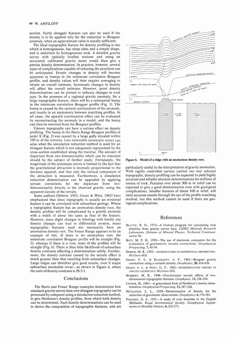
Some authors (Dobrin, 1952, Grant & West, 1965) have emphasised that since topography is usually an erosional feature it can be correlated with subsurface geology. Where a topographic feature has an anomalous density root, the density profiles will be complicated by a gravity anomaly with a width of about the same as that of the feature. However, since slight changes in lithology with hardly any density changes can lead to differential erosion, many topographic features need not necessarily have an anomalous density root. The Fraser Range appears to be an example of this. If there is no anomalous root, the minimum correlation Bouguer profile will be straight (Fig. 5), whereas if there is a root, none of the profiles will be straight (Fig. 6). There is thus little likelihood of subsurface density contrasts affecting a determination subtly. Further•more, the density contrast caused by the terrain effect is much greater than that resulting from subsurface changes. Large ridges can therefore give good results, even if major subsurface anomalies occur-as shown in Figure 6, where the ratio of density contrasts is 28.5: 1.

Conclusions

The Harts and Fraser Range examples demonstrate how standard gravity survey data over elongate topography can be processed by computer using a simulation reduction method, to give Nettleton's density profiles, from which bulk density can be determined. Such density determinations can be used to derive the composition of topographic features, and are

,:2>0 lAJI,\..'I v/c"ff "0 "

~ ~ ;"" .. ~

[~OmGal

s~"\C oeSERVED GRAVITY

UPWARD CONTINUATION BUMP J\.TTP,p..CfIOI'l CONPUTED

G~"''' \~'t 0 SURfACE. 'co" .,0"; .•.•• c .. , ,eo'" ~s"'\IoE. f>.S

[~mGOI

GROUND SURFACE

Flgure 6. Model of a ridge with an anomolous density root.

particularly useful in the interpretation of gravity anomalies. With rigidly controlled surveys carried out over selected topography, density profiling can be expected to yield highly accurate and reliable absolute determinations for millions of tonnes of rock. Features over about 300 m in relief can be expected to give a good determination even with geological complications. Smaller features of about 100 m relief, will yield accurate results through the use ofthe profile matching method, but this method cannot be used if there are geo•logical complications.

References BEATTIE, R. D., 1975---A Fortran program for calculating rock

densities from gravity survey data. CSIRO Minerals Research Laboratory. Division of Mineral Physics. Technical Communi•cation 56.

BOTT, M. P. H., 1959--The use of electronic computers for the evaluation of gravimetric terrain corrections. Geophysical Prospecting, 7,45-54.

DoBRIN, M. B., 1952-INTRODUcrION TO GEOPHYSICAL PROSPEcrING. McGraw-Hill.

GRANT, F. S., & ELSAHARTY, A. F., 1962-Bouguer gravity corrections using a variable density. Geophysics, 28,616-626.

GRANT, F. S., & WEST, G. F., 1965---INTERPRETATION THEORY IN APPLIED GEOPHYSICS. McGraw-Hill.

HUBBERT, M. K., 1948-Gravitational terrain effects of two•dimensional topographic features. Geophysics, 13,226-254.

LINSSER, H., 1965---A generalized form of Nettleton's density deter•illination. Geophysical Prospecting, 13,247-258.

NETTLETON, L. L., 1939--Determination of density for the reduction of gravimeter observations. Geophysics, 4, 176-183.

PARASNIS, D. S., 1951-A study of rock densities in the English Midlands. Royal Astronomical Society, Geophysical Supple•ments to Monthly Notices, 6,252-271.

RUDZKI, M. P., 1905--Sur la determination de la figure de la terre d'apres les mesures de la gravite, Bulletin astronomiaue service B,22.

SIMPSON, S. M ., 19S4-Least squares polynomial fitting to gravitational data and density plotting by digital computers. Geophysics, 19,255-269.

TAKIN, M. & TALWANI, M., 1966--Rapid computation of the gravit•ational attraction of topography on a spherical earth. Geophysical Prospecting. 14,119-142.

TALWANI, M., WORZEL, J. L., & LANDISMAN, M., 1959--Rapid computations for two-dimensional bodies with application to the Mendocino Submarine Fracture Zone, Journal of Geophysical Research. 64,49-59.

VAlKo R. , 1956--Bouguer corrections with varying surface density. Geophysics. 21, 1004-1020.

AUTOMATED DENSITY PROFILING 61