AutoGP: Exploring the Capabilities and Limitations of

Gaussian Process Models

Karl Krauth∗ Edwin V. Bonilla∗ Kurt Cutajar† Maurizio Filippone†

March 7, 2017

Abstract

We investigate the capabilities and limitations of Gaussian process models by jointly exploring threecomplementary directions: (i) scalable and statistically efficient inference; (ii) flexible kernels; and (iii)objective functions for hyperparameter learning alternative to the marginal likelihood. Our approachoutperforms all previously reported gp methods on the standard mnist dataset; performs comparativelyto previous kernel-based methods using the rectangles-image dataset; and breaks the 1% error-ratebarrier in gp models using the mnist8m dataset, showing along the way the scalability of our methodat unprecedented scale for gp models (8 million observations) in classification problems. Overall, ourapproach represents a significant breakthrough in kernel methods and gp models, bridging the gapbetween deep learning approaches and kernel machines.

1 INTRODUCTION

Recent advances in deep learning (dl; LeCun et al., 2015) have revolutionized the application of machinelearning in areas such as computer vision (Krizhevsky et al., 2012), speech recognition (Hinton et al., 2012)and natural language processing (Collobert and Weston, 2008). Although certain kernel-based methods havealso been successful in such domains (Cho and Saul, 2009; Mairal et al., 2014), it is still unclear whetherthese methods can indeed catch up with the recent dl breakthroughs.

Aside from the benefits obtained from using compositional representations, we believe that the maincomponents contributing to the success of dl techniques are: (i) their scalability to large datasets andefficient computation via gpus; (ii) their large representational power; and (iii) the use of well-targetedobjective functions for the problem at hand.

In the kernel world, Gaussian process (gp; Rasmussen and Williams, 2006) models are attractive becausethey are elegant Bayesian nonparametric approaches to learning from data. Nevertheless, besides the lim-itations intrinsic to local kernel machines (Bengio et al., 2005), it is clear that gp-based methods have notfully explored the desirable criteria highlighted above.

Firstly, with regards to (i) scalability, despite recent advances in inducing-variable approaches and vari-ational inference in gp models (Titsias, 2009; Hensman et al., 2013, 2015a; Dezfouli and Bonilla, 2015), thestudy of truly large datasets in problems other than regression and the investigation of gpu-based accelera-tion in gp models are still under-explored areas. We note that these issues are also shared by non-probabilistickernel methods such as support vector machines (svms; Scholkopf and Smola, 2001).

Furthermore, concerning (ii) their representational power, kernel methods have been plagued by theoveruse of very limited kernels such as the squared exponential kernel, also known as the radial-basis-function (rbf) kernel. Even worse, in some gp-based approaches, and more commonly in svms, these havebeen limited to having a single length-scale (a single bandwidth in svm parlance) shared across all inputs

∗School of Computer Science and Engineering, The University of New South Wales, Sydney NSW 2052.†Department of Data Science, EURECOM, France.

1

arX

iv:1

610.

0539

2v3

[st

at.M

L]

6 M

ar 2

017

instead of using different length-scales for each dimensions. The latter approach is commonly known in thegp literature as automatic relevance determination (ard; Mackay, 1994).

Finally, and perhaps most importantly, gp methods have largely ignored defining (iii) well-targetedobjective functions, and instead focused heavily on optimizing the marginal likelihood (Rasmussen andWilliams, 2006, Ch. 5). This includes variational approaches that optimize a lower bound of the marginallikelihood (Titsias, 2009). Although different approaches for hyperparameter learning in gp models arediscussed by Rasmussen and Williams (2006, §5.4.2), and indeed carried out by Sundararajan and Keerthi(2001); Sundararajan et al. (2007); Sundararajan and Keerthi (2008) and more recently by Vehtari et al.(2016), their performance results are somewhat limited by their disregard for other directions of improvement(scalability and greater representational power) mentioned above.

In this work we push the capabilities of gp-models, while also investigating their limitations, by addressingthe above issues jointly. In particular,

1. we develop scalable and statistically efficient inference methods for gp models using gpu computationand stochastic variational inference along with the reparameterization trick (Kingma and Welling,2014);

2. we investigate the flexibility of models using ard kernels for high-dimensional problems, as well as“deep” arc-cosine kernels (Cho and Saul, 2009); and

3. we study the impact of employing a leave-one-out-based objective function on hyperparameter learning.

As we rely on automatic differentiation (Baydin et al., 2015) for the implementation of our model inTensorFlow (Abadi et al., 2015), we refer to our approach as autogp. While we thoroughly evaluate ourclaimed contributions on various regression and classification problems, our most significant results showthat autogp:

• has superior performance to all previously reported gp-based methods on the standard mnist dataset;

• achieves comparable performance to previous kernel-based methods using the rectangles-imagedataset; and

• breaks the 1% error-rate barrier in gp models using the mnist8m dataset, showing along the way thescalability of our approach at unprecedented scale for gp models (8 million observations) in multiclassclassification problems.

Overall, autogp represents a significant breakthrough in kernel methods in general and in gp models inparticular, bridging the gap between deep learning approaches and kernel machines.

2 Related Work

The majority of works related to scalable kernel machines primarily target issues pertaining to the storageand computational requirements of algebraic operations involving kernel matrices. Low-rank approximationsare ubiquitous among these approaches, with the Nystrom approximation being one of the most popularmethods in this category (Williams and Seeger, 2001). Nevertheless, most of these approximations can beunderstood within the unifying probabilistic framework of Quinonero-Candela and Rasmussen (2005).

The optimization of inducing inputs using Nystrom approximations for gps made significant progresswith the work on sparse-gp variational inference in Titsias (2009). This exposed the possibility to developstochastic gradient optimization for gp models (Hensman et al., 2013) and handle non-Gaussian likelihoods(Nguyen and Bonilla, 2014; Dezfouli and Bonilla, 2015; Hensman et al., 2015a; Sheth et al., 2015), whichhas sparked interest in the implementation of scalable inference frameworks such as those in Hensman et al.(2016) and Deisenroth and Ng (2015). These developments greatly improved the generality and applicabilityof gp models to a variety of applications, and our work follows from this line of ideas.

2

Other independent works have focused on kernel design (Wilson and Adams, 2013; Cho and Saul, 2009;Mairal et al., 2014; Wilson et al., 2016). This has sparked some debate as to whether kernel machines canactually compete with deep nets. Evidence suggests that this is possible; notable examples include the workby Huang et al. (2014); Lu et al. (2014). These works also provide insights into the aspects that make kernelmethods less competitive to deep neural networks, namely lack of application specific kernels, and scalabilityat the price of poor approximations. These observations are corroborated by our experiments, which reporthow the combination of these factors impacts performance of gps.

Because gps are probabilistic kernel machines, it is natural to target the optimization of the marginallikelihood. However, alternative objective functions have also been considered, in particular the leave-one-out cross-validation (loo-cv) error. Originally this was done by Sundararajan and Keerthi (2001) forregression; later extended by Sundararajan et al. (2007) to deal with sparse gp formulations; and broadenedby Sundararajan and Keerthi (2008); Vehtari et al. (2016) to handle non-Gaussian likelihoods. While theresults in these papers seem inconclusive as to whether this can generally improve performance, this may allowto better accommodate for incorrect model specifications (Rasmussen and Williams, 2006, §5.4.2). Motivatedby this observation, we explore this direction by extending the variational formulation to optimize a loo-cverror. We also note that none of these previous loo-cv approaches can actually handle large datasets.

3 Gaussian Process Models

We are interested in supervised learning problems where we are given a training dataset of input-outputpairs D = xn,ynnn=1, with xn being a D-dimensional input vector and yn being a P -dimensional output.Our main goal is to learn a probabilistic mapping from inputs to outputs so that for a new input x?, we canestimate the probability of its associated label p(y?|x?).

To this end, we follow a Gaussian process modeling approach (gp; Rasmussen and Williams, 2006),where latent functions are assumed to be distributed according to a gp, and observations are modeled via asuitable conditional likelihood given the latent functions. A function fj is said to be distributed accordingto a Gaussian process with mean function µj(x) and covariance function κj(x,x

′;θj), which we denote withfj ∼ GP(µj(x), κj(x,x

′;θj)), if any subset of function values follow a Gaussian distribution.Since we are dealing with multiple outputs yn, we follow the standard practice of considering Q

underlying latent functions fjQj=1 which are drawn independently from zero-mean gp priors along withi.i.d. conditional likelihood models. Such a modeling approach encompasses a large class of machine learningproblems, including gp-regression, gp-classification and modeling of count data (Rasmussen and Williams,2006).

Consequently, when realized at the observed data, our probabilistic model is given by:

p(f |X,θ) =

Q∏j=1

p(f·j |X,θj) =

Q∏j=1

N (f·j ; 0,Kj), (1)

p(y|f) =

N∏n=1

p(yn|fn·), (2)

where f is the (N × Q)-dimensional vector of all latent function values; f·j = fj(xn)Nn=1 denotes thelatent function values corresponding to the jth gp; Kj is the covariance matrix obtained by evaluatingthe covariance function κj(·, ·;θ) at all pairs of training inputs; y is the vector of all (N × P ) output

observations, with yn being nth output observation, and fn· = fj(xn)Qj=1 being the corresponding vectorof latent function values. We refer to the covariance parameters θ as the hyperparameters.

One commonly used covariance function is the so-called squared exponential (or rbf kernel):

κ(x,x′;θ) = σ2 exp

(−

D∑i=1

(xi − x′i)2

`2i

), (3)

3

where θ = σ2, `21, . . . , `2D and D is the input dimensionality. When all the lengthscales, `i, are constrained

to be the same we refer to the above kernel as isotropic; otherwise, we refer to it as the squared exponentialcovariance with automatic relevance determination (ard).

3.1 Inference Problems

The main inference problems in gp models are (i) estimation of the posterior over the latent functionsp(f |X,y,θ) and subsequent estimation of the predictive distribution p(y?|x?,X,y,θ); and (ii) inference overthe hyperparameters θ.

For general likelihood models, both inference problems are analytically intractable, as they require thecomputation of non-trivial high-dimensional integrals. Furthermore, even for the simplest case when the con-ditional likelihood is Gaussian, evaluating the posterior and hyperparameter estimation is computationallyprohibitive, as they entail time and memory requirements of O(N3) and O(N2) respectively.

In addition to dealing with general likelihood models and scalability issues, the performance of gp models(and kernel machines in general), is highly dependent on the covariance function (or kernel) used. Mostprevious work on gp methods and svms in the machine learning literature, use the squared exponentialkernel in Equation (3). Furthermore, especially in high dimensions, this kernel is constrained to its isotropicversion. As pointed out by Bengio et al. (2005), such an approach is severely limited by the curse ofdimensionality when learning complex functions.

Finally, the estimation of hyper-parameters based solely on marginal likelihood optimization can be verysensitive to model misspecification, with predictive approaches such as those in Sundararajan and Keerthi(2001) being seemingly more appealing for this task, especially in problems such as classification, where weare ultimately interested in having lower error rates and better calibrated predictive probabilities.

In the following sections, we show how to deal with the above issues, namely non-Gaussian likelihoodmodels and scalability; more flexible kernels; and better objective functions for hyperparameter learning,with the endmost goal of improving performance significantly over current gp approaches.

4 Automated Variational Inference

In this section we detail our method for scalable and statistically efficient inference in Gaussian processmodels with general likelihoods as specified by Equations (1) and (2). We adopt the variational frameworkof Dezfouli and Bonilla (2015), which we prefer over the mcmc method of Hensman et al. (2015b) as weavoid the sampling overhead which is especially significant in very large datasets.

4.1 Augmented Model

In order to have a scalable inference framework, we augment our prior with M inducing variables u·j perlatent process and corresponding inducing inputs Zj such that,

p(u) =

Q∏j=1

N (u·j ; 0,Kjzz), (4)

p(f |u) =

Q∏j=1

N (f·j ; µj , Kj), where (5)

µj = Kjxz(Kj

zz)−1u·j , and (6)

Kj = Kjxx −AjK

jzx with Aj = Kj

xz(Kjzz)−1, (7)

where Kjuv is the covariance matrix obtained by evaluating the covariance function κj(·, ·;θ) at all pairwise

columns of matrices U and V. We note that this prior is equivalent to that defined in Equation (1), which isobtained by integrating out u from the joint p(f ,u). However, as originally proposed by Titsias (2009), having

4

an explicit representation of u will allow us to derive a scalable variational framework without additionalassumptions on the train or test conditional distributions (Quinonero-Candela and Rasmussen, 2005).

We now define our approximate joint posterior distribution as:

q(f ,u|λ)def= p(f |u)q(u|λ), with (8)

q(u|λ) =

K∑k=1

πk

Q∏j=1

N (u·j ; mkj ,Skj), (9)

where p(f |u) is the conditional prior given in Equation (4) as variational parameters. q(u|λ) is our variationalposterior with λ = πk,mkj ,Skj. Note that we assume a variational posterior in the form of a mixture foradded flexibility compared to using a single distribution.

4.2 Evidence Lower Bound

Such a definition of the variational posterior allows for simplification of the log-evidence lower bound (Lelbo)such that no O(N3) operations are required,

Lelbo(λ,θ) = −KL(q(u|λ)‖p(u))+

N∑n=1

K∑k=1

πkEqk(n)(fn·|λk)[log p(yn|fn·)], (10)

where KL(q‖p) denotes the KL divergence between distributions q and p; Ep(X)[g(X)] denotes the expectationof g(X) over distribution p(X); and qk(n)(fn·|λk) is a Q-dimensional diagonal Gaussian with means andvariances given by

bknj = aTjnmkj , (11)

σ2knj = [Kj ]n,n + aT

jnSkjajn, (12)

where ajndef= [Aj ]:,n denotes the M -dimensional vector corresponding to the nth column of matrix Aj ; Kj

and Aj are given in Equation (7); and, [Kj ]n,n denotes the (n, n)th entry of matrix Kj .In order to compute the log-evidence lower bound in Equation (10) and its gradients, we use Jensen’s

inequality to bound the KL term (as in Dezfouli and Bonilla, 2015) and estimate the expected likelihoodterm using Monte Carlo (mc).

4.3 The Reparameterization Trick

One of the key properties of the log-evidence lower bound in Equation (10) is its decomposition as a sumof expected likelihood terms on the individual observations. This allows for the applicability of stochasticoptimization methods and, therefore, scalability to very large datasets.

Due to the expectation term in the expression of the Lelbo, gradients of the Lelbo need to be estimated.Dezfouli and Bonilla (2015) follow a similar approach to that in general black-box variational methods(Ranganath et al., 2014), and use the property ∇λEq(f |λ)[log p(y|f)] = Eq(λ)[∇λ log q(f |λ) log p(y|f)] andMonte Carlo (mc) sampling to produce unbiased estimates of these gradients. While such an approach istruly black-box in that it does not require detailed knowledge of the conditional likelihood and its gradients,the estimated gradients may have significantly large variance, which could hinder the optimization process.In fact, Dezfouli and Bonilla (2015) and Bonilla et al. (2016) use variance-reduction techniques (Ross, 2006,§8.2) to ameliorate this effect. Nevertheless, the experiments in Bonilla et al. (2016) on complex likelihoodfunctions such as those in Gaussian process regression networks (gprns; Wilson et al., 2012) indicate thatsuch techniques may be insufficient to control the stability of the optimization process, and a large numberof mc samples may be required.

5

In contrast, if one is willing to relax the constraints of a truly black-box approach by having access to theimplementation of the conditional likelihood and its gradients, then a simple trick proposed by Kingma andWelling (2014) can significantly reduce the variance in the gradients and make the stochastic optimizationof Lelbo much more practical. This has come to be known as the reparameterization trick.

We now present explicit expressions of our estimated Lelbo, focusing on an individual expected likelihoodterm in Equation (10). Thus, the individual expectations can be estimated as:

εknj ∼ N (0, 1), (13)

f(k,i)nj = bknj + σknjεknj , j = 1, . . . , Q, (14)

L(n)ell =

1

S

K∑k=1

πk

S∑i=1

log p(yn|f (k,i)n· ), (15)

where S is the number of mc samples and f(k,i)nj is an element in the vector of latent functions f

(k,i)n· .

4.4 Mini-Batch Optimization

We can now obtain unbiased estimates of the gradients of Lelbo to use in mini-batch stochastic optimization.In particular, for a mini-batch Ω of size B we have that the estimated gradient is given by:

∇ηLelbo = −∇ηKL(q(u|λ)‖p(u)) +N

B

∑n∈Ω

∇ηL(n)ell ,

where η ∈ λ,θ; θ now includes not only the covariance parameters, but also the inducing inputs acrossall latent processes Zj . The corresponding gradients are obtained through automatic differentiation usingTensorFlow.

4.5 Full Approximate Posterior

An important characteristic of our approach is that, unlike most previous work that uses stochastic opti-mization in variational inference along with the reparameterization trick (see e.g. Kingma and Welling, 2014;Dai et al., 2016), we do not require a fully factorized approximate posterior to estimate our gradients usingonly simple scalar transformations of uncorrelated Gaussian samples, as given in Equation (14). Indeed, theposterior over the latent functions is fully correlated and is given in the Appendix. This result is a propertyinherited from the original framework of Nguyen and Bonilla (2014) and Dezfouli and Bonilla (2015), whoshowed that, even when having a full approximate posterior, only expectations over univariate Gaussiansare required in order to estimate the expected log likelihood term in Lelbo.

5 Flexible Kernels

We now turn our attention to increase the flexibility of gp models through the investigation of kernels beyondthe isotropic rbf kernel. This is a complementary direction for exploring the capabilities of gp models, but itbenefits from the results of the previous section in terms of large-scale inference and computation of gradientsvia (automatic) back-propagation.

For the rbf kernel, we limit our experiments to the automatic relevance determination (ard) setting inEquation (3), including problems of large input dimensionality such as mnist and cifar10. Furthermore,given the interesting results reported by Cho and Saul (2009), we also investigate their arc-cosine kernel,which was proposed as a kernel that mimics the computation of neural networks. We give the mathematicaldetails of the arc-cosine kernel in the Appendix.

6

Algorithm 1 Loo-based hyperparameter learning.

repeatrepeat

(θ,λ)← (θ,λ) + α∇θ,λLelbo(θ,λ)until satisfiedrepeat

θ ← θ + α∇θLoo(θ)until satisfied

until satisfied

6 Leave-One-Out Learning

Here we focus on the average leave-one-out log predictive probability for hyper-parameter learning, as analternative to optimization of the marginal likelihood. This can be particularly useful in problems suchas classification where one is mainly interested in having lower error rates and better calibrated predictiveprobabilities.

This objective function is obtained by leaving one datapoint out of the training set and computing itslog predictive probability when training on the other points; the resulting values are then averaged acrossall the datapoints. Interestingly, in our gp model this can be computed without the need for training Ndifferent models, as the resulting expression is given by:

Loo(θ) ≈ − 1

N

N∑n=1

log

∫q(fn·|D,λ,θ)

p(yn|fn·)dfn·, (16)

where the approximation stems from using the variational marginal posterior q(fn·|D,θ) instead of the truemarginal posterior p(fn·|D,θ) for datapoint n. We also note that we have made explicit the dependencyof the posterior on all the data. The derivation of this expression is given in the Appendix. Since Loo(θ)contains an expectation with respect to the marginal posterior we can also estimate it via mc sampling.

Equation (16) immediately suggests an alternating optimization scheme where we estimate the approx-imate posterior q(fn·|D,θ) through optimization of Lelbo, as described in §4, and then learn the hyperpa-rameters via optimization of Loo. Algorithm 1 illustrates such an alternating scheme for hyperparameterlearning in our model using the leave-one-out objective and vanilla stochastic gradient descent (sgd), where

Lelbo and Loo denote estimates of the corresponding objectives when using mini-batches.

7 Experiments

We evaluate autogp across various datasets with number of observations ranging from 12, 000 to 8.1M andinput dimensionality between 31 and 3072. The aim of this section is (i) to demonstrate the effectiveness ofthe re-parametrization trick in reducing the number of samples needed to estimate the expected log likelihood;(ii) to evaluate non-isotropic kernels across a large number of dimensions; (iii) to assess the performanceobtained by loo-cv hyperparameter learning; and (iv) to analyze the performance of autogp as a functionof time. Details of the experimental set-up can be found in the supplementary material.

7.1 Statistical Efficiency

For our first experiment we look at the behavior of our model as we vary the number of samples used toestimate the expected log likelihood. We trained our model on the sarcos dataset (Vijayakumar and Schaal,2000), an inverse dynamics problem for a seven degrees-of-freedom anthropomorphic robot arm.

We used the Gaussian process regression network (gprn) model of Wilson et al. (2012) as our likelihoodfunction. Bonilla et al. (2016) found that gprns require a large number of samples (10, 000) to yield stable

7

0 500 1000 1500 2000

Epochs

0.00

0.05

0.10

0.15

0.20

0.25

0.30

MSSE

Samples10

100

1000

10000

Figure 1: The mean standardized square error (msse) of autogp for different number of mc samples on thesarcos dataset. The msse was averaged across all 7 joints and 50 inducing inputs were used to train themodel. An epoch represents a single pass over the entire training set.

optimization of the Lelbo in their method. This is most likely due to the increased variance induced bymultiplying latent samples together. The high variance of this likelihood model makes it an ideal candidatefor us to evaluate how the performance of autogp varies with the number of samples.

As shown in Figure 1, increasing the number of samples decreased the number of epochs it took forour model to converge; however, our model always converged to the same optimal value. This is in starkcontrast to savigp (Bonilla et al., 2016) which was able to converge to the optimal value of 0.0195 with 10, 000samples, but converged to sub-optimal values (> 0.05) as the number of samples was lowered. This showsthat our mc estimator is significantly more stable than savigp’s black-box estimator, without requiring anyvariance reduction methods. In practice, reducing the number of samples leads to an improved runtime. Agradient update using 10, 000 samples takes around 0.17 seconds, whereas an update using 10 samples onlytakes around 0.03 seconds, which makes up for the extra epochs needed to converge.

7.2 Kernel Performance

In this section we compare the performance of autogp across two different kernels on a high-dimensionaldataset. We trained our model on the rectangles-image dataset (Larochelle et al., 2007) which is a binaryclassification task that was created to compare shallow models (e.g. svms), and deep learning architectures.The task involves recognizing whether a rectangle has a larger width or height. Randomized images wereoverlayed behind and over the rectangles, which makes this task particularly challenging.

We compare the multilayer arc-cosine kernel (arc-cosine) described by Cho and Saul (2009) with anrbf kernel with automatic relevance determination (rbf-ard). arc-cosine was devised to mimic thearchitecture of deep neural networks through successive kernel compositions, and has shown good resultswhen combined with non-Bayesian kernel machines (Cho and Saul, 2009). Unlike arc-cosine, rbf-ard iscommonly used with Gaussian processes (Hensman et al., 2013). However, rbf-ard has not been appliedto large-scale datasets with a large input dimensionality due to limitations in scalability. Given that ourimplementation uses automatic differentiation, and is thus able to efficiently compute gradients, we can userbf-ard with no noticeable performance overhead.

We trained our model using 10, 200, and 1000 inducing points across both kernels. We experimentedwith various different depths and degrees for arc-cosine and found that 3 layers and a degree of 1 workedbest with autogp. As such, we ran all arc-cosine experiments with these settings.

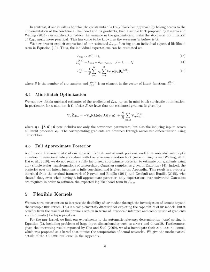
For reference, Cho and Saul (2009) report an error rate of 22.36% using svms with arc-cosine. Larochelleet al. (2007) report error rates of 24.04% on svms with a simple rbf kernel and 22.50% with a deep belief

8

ARD COS SVM DBN

10 200 1000 10 200 10000

10

20

SFer

ror r

ate

Figure 2: Error rates for binary classification using a logistic likelihood on rectangles-image. ARD andCOS refer to autogp with a rbf-ard kernel, and a 3-layer arc-cosine kernel of degree 1 respectively. DBNrefers to a 3-layer deep belief network and svm denotes a support vector machine with a arc-cosine kernelof depth 6 and degree 0.

network with 3 hidden layers (DBN).Figure 2 shows that autogp is competitive with previous approaches, except when using 10 inducing

points. Our results also show that rbf-ard performs comparatively (and sometimes better) than arc-cosine. This is likely because arc-cosine is better suited to deep architectures, such as the multilayerkernel machine of Cho and Saul (2009).

7.3 LOO-CV Hyperparameter Learning

In this section we analyze our approach when learning hyperparameters via optimization of the leave-one-out objective (Loo), as described in §6, and compare it with the standard variational method that learns

hyperparameters via sole optimization of the variational objective (Lelbo). To this end, we use the mnistdataset using 10, 200, and 1000 inducing points and the rbf-ard kernel across all settings.

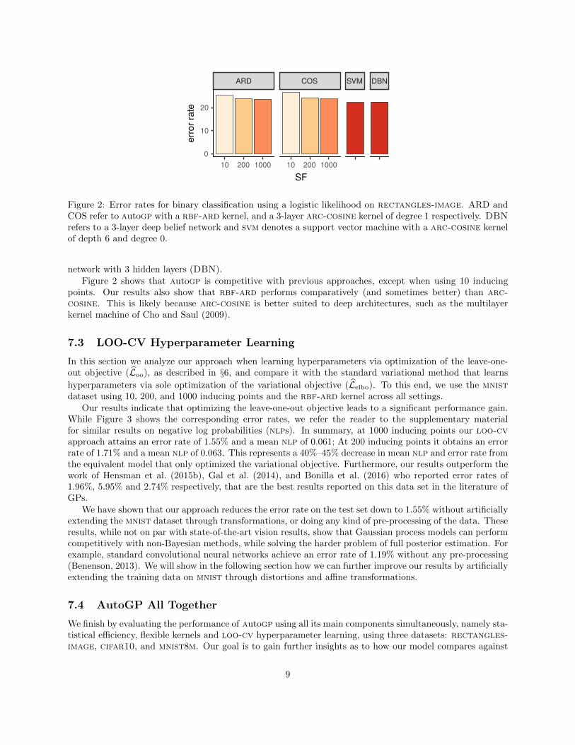
Our results indicate that optimizing the leave-one-out objective leads to a significant performance gain.While Figure 3 shows the corresponding error rates, we refer the reader to the supplementary materialfor similar results on negative log probabilities (nlps). In summary, at 1000 inducing points our loo-cvapproach attains an error rate of 1.55% and a mean nlp of 0.061; At 200 inducing points it obtains an errorrate of 1.71% and a mean nlp of 0.063. This represents a 40%–45% decrease in mean nlp and error rate fromthe equivalent model that only optimized the variational objective. Furthermore, our results outperform thework of Hensman et al. (2015b), Gal et al. (2014), and Bonilla et al. (2016) who reported error rates of1.96%, 5.95% and 2.74% respectively, that are the best results reported on this data set in the literature ofGPs.

We have shown that our approach reduces the error rate on the test set down to 1.55% without artificiallyextending the mnist dataset through transformations, or doing any kind of pre-processing of the data. Theseresults, while not on par with state-of-the-art vision results, show that Gaussian process models can performcompetitively with non-Bayesian methods, while solving the harder problem of full posterior estimation. Forexample, standard convolutional neural networks achieve an error rate of 1.19% without any pre-processing(Benenson, 2013). We will show in the following section how we can further improve our results by artificiallyextending the training data on mnist through distortions and affine transformations.

7.4 AutoGP All Together

We finish by evaluating the performance of autogp using all its main components simultaneously, namely sta-tistical efficiency, flexible kernels and loo-cv hyperparameter learning, using three datasets: rectangles-image, cifar10, and mnist8m. Our goal is to gain further insights as to how our model compares against

9

VAR LOO

0.00

0.01

0.02

0.03

10 200 1000 10 200 1000

num inducing

erro

r ra

teFigure 3: Error rates of autogp for multiclass classification using a softmax likelihood on mnist. VAR refersto learning using only the variational objective Lelbo, while LOO refers to learning hyperparameters usingthe leave-one-out objective Loo.

0 2 4 6 8 10

Hours

0.00

0.01

0.02

0.03

0.04

0.05

err

or

rate

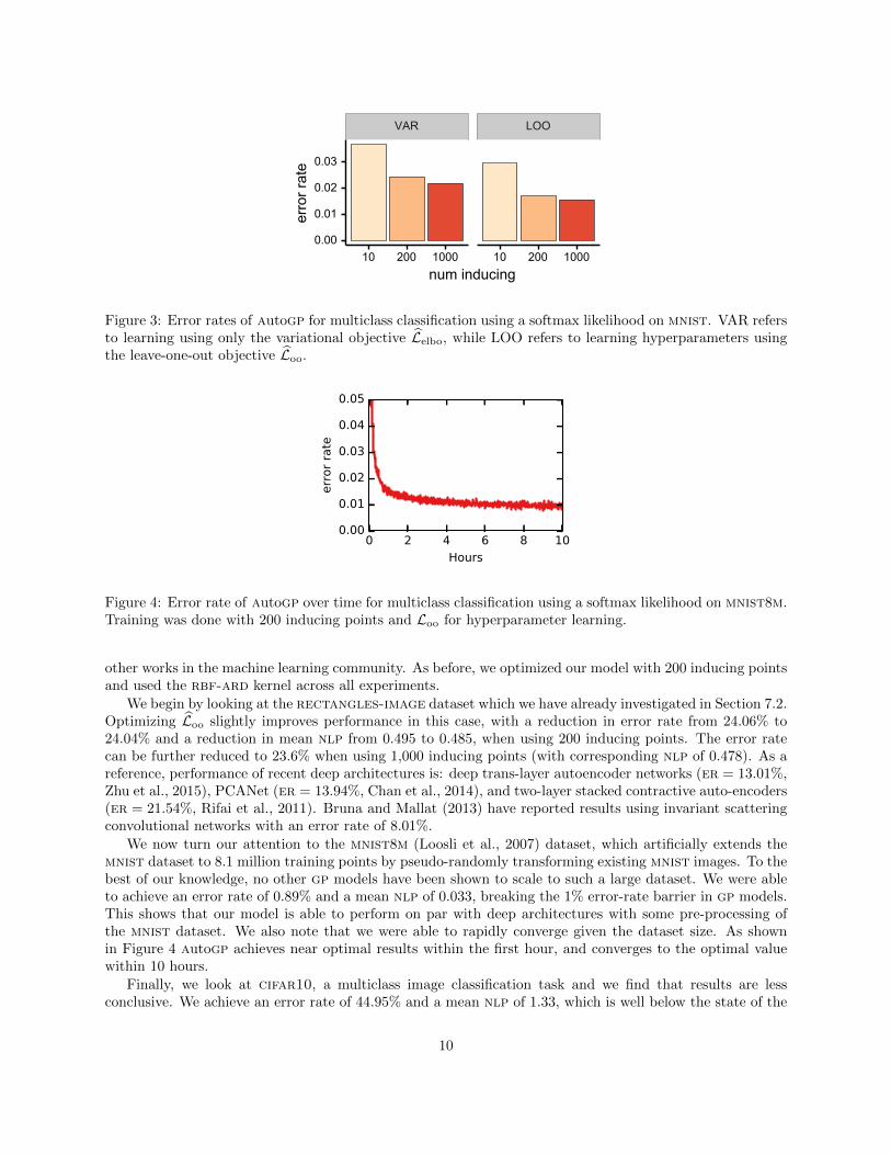
Figure 4: Error rate of autogp over time for multiclass classification using a softmax likelihood on mnist8m.Training was done with 200 inducing points and Loo for hyperparameter learning.

other works in the machine learning community. As before, we optimized our model with 200 inducing pointsand used the rbf-ard kernel across all experiments.

We begin by looking at the rectangles-image dataset which we have already investigated in Section 7.2.Optimizing Loo slightly improves performance in this case, with a reduction in error rate from 24.06% to24.04% and a reduction in mean nlp from 0.495 to 0.485, when using 200 inducing points. The error ratecan be further reduced to 23.6% when using 1,000 inducing points (with corresponding nlp of 0.478). As areference, performance of recent deep architectures is: deep trans-layer autoencoder networks (er = 13.01%,Zhu et al., 2015), PCANet (er = 13.94%, Chan et al., 2014), and two-layer stacked contractive auto-encoders(er = 21.54%, Rifai et al., 2011). Bruna and Mallat (2013) have reported results using invariant scatteringconvolutional networks with an error rate of 8.01%.

We now turn our attention to the mnist8m (Loosli et al., 2007) dataset, which artificially extends themnist dataset to 8.1 million training points by pseudo-randomly transforming existing mnist images. To thebest of our knowledge, no other gp models have been shown to scale to such a large dataset. We were ableto achieve an error rate of 0.89% and a mean nlp of 0.033, breaking the 1% error-rate barrier in gp models.This shows that our model is able to perform on par with deep architectures with some pre-processing ofthe mnist dataset. We also note that we were able to rapidly converge given the dataset size. As shownin Figure 4 autogp achieves near optimal results within the first hour, and converges to the optimal valuewithin 10 hours.

Finally, we look at cifar10, a multiclass image classification task and we find that results are lessconclusive. We achieve an error rate of 44.95% and a mean nlp of 1.33, which is well below the state of the

10

art, with some models achieving less than 10% error rate. However, we note that we still compare favorablyto svms which have been shown to achieve error rates of 57.7% (Le et al., 2013). We also perform on parwith older deep architectures (Rifai et al., 2011). We believe these results provide a strong motivation forinvestigating application-specific kernels (such as those studied by Mairal et al., 2014) in gp models.

Table 1: Test error rate and mean nlp of autogp trained with 200 inducing points on various datasets. TheLoo objective was used for hyperparameter learning

Dataset Error rate mean nlp

rectangles-image 24.06% 0.485mnist8m 0.89% 0.033cifar10 44.95% 1.333

8 CONCLUSIONS & DISCUSSION

We have developed autogp, an inference framework for gp models that pushes the performance of currentgp methods by exploring three complementary directions: (i) scalable and statistically efficient variationalinference; (ii) flexible kernels; and (iii) objective functions for hyperparameter learning alternative to themarginal likelihood.

We have shown that our framework outperforms all previous gp approaches on mnist; achieves com-parable performance to previous kernel approaches on the rectangles-image dataset; and can break the1% error barrier using mnist8m. Overall, this represents a significant breakthrough in Gaussian processmethods and kernel machines. While our results on cifar10 are well below the state-of-the-art achievedwith deep learning, we believe we can further reduce the gap between kernel machines and deep architecturesby using application-specific kernels such as those recently proposed by Mairal et al. (2014).

A Details of Full Posterior Distribution

The full posterior distribution over the latent functions is given by:

q(f |λ) =

K∑k=1

πk

Q∏j=1

N (f·j ; bkj ,Σkj), where (17)

bkj = Ajmkj , and (18)

Σkj = Kj + AjSkjATj . (19)

B Details of The Arc-Cosine Kernel

Cho and Saul (2009) define an arc-cosine kernel of degree d and depth l using the following recursion:

κ(l+1)d (x,x′) =

1

π

(κ

(l)d (x,x)κ

(l)d (x′,x′)

)d/2

Jd(φ(l)d ) (20)

κ(1)d (x,x′) =

1

π‖x‖d‖x′‖dJd(φ) (21)

11

where

φ(l)d = cos−1

(κ

(l)d (x,x′)

(κ

(l)d (x,x)κ

(l)d (x′,x′)

)−1/2)

(22)

Jd(φ) = (−1)d(sinφ)2d+1

(1

sinφ

∂

∂φ

)d(π − φsinφ

)(23)

φ = cos−1

(x · x′

‖x‖‖x′‖

). (24)

C Derivation of Leave-One-Out Objective

In this section we derive an expression for the leave-one-out objective and show that this does not requiretraining of N models. A similar derivation can be found in Vehtari et al. (2016). Let D¬n = X¬n,y¬n bethe dataset resulting from removing observation n. Then our leave-one-out objective is given by:

Loo(θ) =1

N

N∑n=1

log p(yn|xn,D¬n,θ). (25)

We now that the marginal posterior can be computed as:

p(fn·|D) = p(fn·|X¬n,y¬n,xn,yn) =p(yn|fn·)p(fn·|xn,D¬n)

p(yn|xn,D¬n,θ)(26)

and re-arranging terms ∫p(fn·|xn,D¬n,θ)dfn· =

∫p(fn·|D,θ)p(yn|xn,D¬n,θ)

p(yn|fn·)dfn· (27)

p(yn|xn,D¬n,θ) = 1/

∫p(fn·|D,θ)

p(yn|fn·)dfn· (28)

log p(yn|xn,D¬n;θ) = − log

∫p(fn·|D,θ)

p(yn|fn·)dfn·, (29)

and substituting this expression in Equation (25) we have

Loo(θ) = − 1

N

N∑n=1

log

∫p(fn·|D,θ)

1

p(yn|fn·)dfn·. (30)

We see that the objective only requires estimation of the marginal posterior p(fn·|D,θ), which we canapproximate using variational inference, hence:

Loo(θ) ≈ − 1

N

N∑n=1

log

∫q(fn·|D,θ)

1

p(yn|fn·)dfn·, (31)

where q(fn·|D,θ) is our approximate variational posterior.

D Additional Details of Experiments

D.1 Experimental Set-up

The datasets used are described in Table 2. We trained our model stochastically using the rmsprop optimizerprovided by TensorFlow (Abadi et al., 2015) with a learning rate of 0.003 and mini-batches of size 1000. We

12

Table 2: The datasets used in the experiments and the corresponding models used. Ntrain, Ntest, D are thenumber of training points, test points and input dimensions respectively.

Dataset Ntrain Ntest D Model

sarcos 44, 484 4, 449 21 gprnrectangles-image 12, 000 50, 000 784 Binary classification

mnist 60, 000 10, 000 784 Multi-class classificationcifar10 50, 000 10, 000 3072 Multi-class classificationmnist8m 8.1M 10, 000 784 Multi-class classification

VAR LOO

0.00

0.05

0.10

10 200 1000 10 200 1000

num inducing

NLP

Figure 5: nlp for multiclass classification using a softmax likelihood model on the mnist dataset. VARshows the performance of autogp where all parameters are learned using only the variational objectiveLelbo, while LOO represents the performance of autogp when hyperparameters are learned using the leave-one-out objective Loo.

initialized inducing point locations by using the k-means clustering algorithm, and initialized the posteriormean to a zero vector, and the posterior covariances to identity matrices. When jointly optimizing Loo andLelbo, we alternated between optimizing each objective for 100 epochs. Unless otherwise specified we used100 Monte-Carlo samples to estimate the expected log likelihood term.

All timed experiments were performed on a machine with an Intel(R) Core(TM) i5-4460 CPU, 24GB ofDDR3 RAM, and a GeForce GTX1070 GPU with TensorFlow 0.10rc.

D.2 Additional Results

Figure 5 shows the nlp for our evaluation of the loo-cv-based hyperparameter learning. As with the errorrates described in the main text, the nlp obtained with loo-cv are significantly better than those obtainedwith a purely variational approach.

References

Martın Abadi, Ashish Agarwal, Paul Barham, et al. TensorFlow: Large-scale machine learning on heteroge-neous systems, 2015.

Atilim Gunes Baydin, Barak A Pearlmutter, Alexey Andreyevich Radul, and Jeffrey Mark Siskind. Auto-matic differentiation in machine learning: a survey. arXiv preprint arXiv:1502.05767, 2015.

Rodrigo Benenson. What is the class of this image? discover the current state of the art in objects classifi-

13

cation. http://rodrigob.github.io/are_we_there_yet/build/classification_datasets_results.

html, 2013. [Online; accessed 13-October-2016].

Yoshua Bengio, Olivier Delalleau, and Nicolas L Roux. The curse of highly variable functions for local kernelmachines. In Neural Information Processing Systems, 2005.

Edwin V Bonilla, Karl Krauth, and Amir Dezfouli. Generic inference in latent Gaussian process models.arXiv preprint arXiv:1609.00577, 2016.

Joan Bruna and Stephane Mallat. Invariant scattering convolution networks. IEEE Transactions on PatternAnalysis and Machine Intelligence, pages 1872–1886, 2013.

Tsung-Han Chan, Kui Jia, Shenghua Gao, Jiwen Lu, Zinan Zeng, and Yi Ma. PCANet: A simple deeplearning baseline for image classification? arXiv preprint arXiv:1404.3606, 2014.

Youngmin Cho and Lawrence K. Saul. Kernel methods for deep learning. In Neural Information ProcessingSystems. 2009.

Ronan Collobert and Jason Weston. A unified architecture for natural language processing: Deep neuralnetworks with multitask learning. In International Conference on Machine Learning, 2008.

Zhenwen Dai, Andreas Damianou, Javier Gonzalez, and Neil Lawrence. Variational Auto-encoded DeepGaussian Processes. In International Conference on Learning Representations, 2016.

Marc Peter Deisenroth and Jun Wei Ng. Distributed Gaussian processes. In International Conference onMachine Learning, 2015.

Amir Dezfouli and Edwin V. Bonilla. Scalable inference for Gaussian process models with black-box likeli-hoods. In Neural Information Processing Systems. 2015.

Yarin Gal, Mark van der Wilk, and Carl Rasmussen. Distributed variational inference in sparse Gaussianprocess regression and latent variable models. In Neural Information Processing Systems. 2014.

James Hensman, Nicolo Fusi, and Neil D Lawrence. Gaussian processes for big data. In Uncertainty inArtificial Intelligence, 2013.

James Hensman, Alexander Matthews, and Zoubin Ghahramani. Scalable variational Gaussian processclassification. In Artificial Intelligence and Statistics, 2015a.

James Hensman, Alexander G Matthews, Maurizio Filippone, and Zoubin Ghahramani. MCMC for varia-tionally sparse Gaussian processes. In Neural Information Processing Systems. 2015b.

James Hensman, Alexander G. de G. Matthews, Alexis Boukouvalas, Keisuke Fujii, Pablo Leon, ValentineSvensson, and Mark van der Wilk. GPflow. https://github.com/GPflow/GPflow, 2016.

Geoffrey Hinton, Li Deng, Dong Yu, George E Dahl, Abdel-rahman Mohamed, Navdeep Jaitly, AndrewSenior, Vincent Vanhoucke, Patrick Nguyen, Tara N Sainath, et al. Deep neural networks for acous-tic modeling in speech recognition: The shared views of four research groups. IEEE Signal ProcessingMagazine, 29(6):82–97, 2012.

Po-Sen Huang, Haim Avron, Tara N. Sainath, Vikas Sindhwani, and Bhuvana Ramabhadran. Kernel methodsmatch deep neural networks on TIMIT. In IEEE International Conference on Acoustics, Speech and SignalProcessing, 2014.

Diederik P Kingma and Max Welling. Auto-encoding variational Bayes. In International Conference onLearning Representations, 2014.

14

Alex Krizhevsky, Ilya Sutskever, and Geoffrey E Hinton. Imagenet classification with deep convolutionalneural networks. In Neural Information Processing Systems, pages 1097–1105, 2012.

Hugo Larochelle, Dumitru Erhan, Aaron Courville, James Bergstra, and Yoshua Bengio. An empiricalevaluation of deep architectures on problems with many factors of variation. In International Conferenceon Machine Learning, 2007.

Quoc V. Le, Tamas Sarlos, and Alexander J. Smola. Fastfood - computing Hilbert space expansions inloglinear time. In International Conference on Machine Learning, 2013.

Yann LeCun, Yoshua Bengio, and Geoffrey Hinton. Deep learning. Nature, 521(7553):436–444, 2015.

Gaelle Loosli, Stephane Canu, and Leon Bottou. Training invariant support vector machines using selectivesampling. In Large Scale Kernel Machines, pages 301–320. MIT Press, Cambridge, MA., 2007.

Zhiyun Lu, Avner May, Kuan Liu, Alireza Bagheri Garakani, Dong Guo, Aurelien Bellet, Linxi Fan, MichaelCollins, Brian Kingsbury, Michael Picheny, and Fei Sha. How to scale up kernel methods to be as goodas deep neural nets. CoRR, abs/1411.4000, 2014.

D. J. C. Mackay. Bayesian methods for backpropagation networks. In E. Domany, J. L. van Hemmen, andK. Schulten, editors, Models of Neural Networks III, chapter 6, pages 211–254. Springer, 1994.

Julien Mairal, Piotr Koniusz, Zaid Harchaoui, and Cordelia Schmid. Convolutional kernel networks. InNeural Information Processing Systems, pages 2627–2635, 2014.

Trung V. Nguyen and Edwin V. Bonilla. Automated variational inference for Gaussian process models. InNeural Information Processing Systems. 2014.

Joaquin Quinonero-Candela and Carl Edward Rasmussen. A unifying view of sparse approximate Gaussianprocess regression. Journal of Machine Learning Research, 6:1939–1959, 2005.

Rajesh Ranganath, Sean Gerrish, and David M. Blei. Black box variational inference. In Artificial Intelligenceand Statistics, 2014.

Carl Edward Rasmussen and Christopher K. I. Williams. Gaussian processes for machine learning. TheMIT Press, 2006.

Salah Rifai, Pascal Vincent, Xavier Muller, Xavier Glorot, and Yoshua Bengio. Contractive auto-encoders:Explicit invariance during feature extraction. In International Conference on Machine Learning, 2011.

Sheldon M Ross. Simulation. Burlington, MA: Elsevier, 2006.

Bernhard Scholkopf and Alexander J Smola. Learning with kernels: support vector machines, regularization,optimization, and beyond. MIT press, 2001.

Rishit Sheth, Yuyang Wang, and Roni Khardon. Sparse variational inference for generalized GP models. InInternational Conference on Machine Learning, 2015.

S Sundararajan and S Sathiya Keerthi. Predictive approaches for choosing hyperparameters in Gaussianprocesses. Neural Computation, 13(5):1103–1118, 2001.

S. Sundararajan and S. Sathiya Keerthi. Predictive approaches for Gaussian process classifier model selection.Technical report, 2008.

S. Sundararajan, S. Sathiya Keerthi, and Shirish Shevade. Predictive approaches for sparse Gaussian processregression. Technical report, 2007.

Michalis Titsias. Variational learning of inducing variables in sparse Gaussian processes. In Artificial Intel-ligence and Statistics, 2009.

15

Aki Vehtari, Tommi Mononen, Ville Tolvanen, Tuomas Sivula, and Ole Winther. Bayesian leave-one-outcross-validation approximations for Gaussian latent variable models. Journal of Machine Learning Re-search, 17(103):1–38, 2016.

Sethu Vijayakumar and Stefan Schaal. Locally weighted projection regression: An O(n) algorithm for incre-mental real time learning in high dimensional space. In International Conference on Machine Learning,2000.

Christopher Williams and Matthias Seeger. Using the Nystrom method to speed up kernel machines. InNeural Information Processing Systems, 2001.

Andrew G. Wilson, David A. Knowles, and Zoubin Ghahramani. Gaussian process regression networks. InInternational Conference on Machine Learning, 2012.

Andrew Gordon Wilson and Ryan Prescott Adams. Gaussian process kernels for pattern discovery andextrapolation. In International Conference on Machine Learning, pages 1067–1075, 2013.

Andrew Gordon Wilson, Zhiting Hu, Ruslan Salakhutdinov, and Eric P. Xing. Deep kernel learning. InArtificial Intelligence and Statistics, 2016.

Wentao Zhu, Jun Miao, Laiyun Qing, and Xilin Chen. Deep trans-layer unsupervised networks for represen-tation learning. arXiv preprint arXiv:1509.08038, 2015.

16