Auto configuration dans LTE : procédés de mesure de · PDF fileAu cours de la...

INP Grenoble - ENSIMAG École Nationale Supérieure d’Informatique et de Mathématiques Appliquées de

Grenoble

Rapport de projet de fin d’études

Effectué chez ALCATEL-LUCENT BELL LABS

Auto configuration dans LTE : procédés de mesure de l’occupation du canal radio pour

une utilisation optimisée du spectre

Juan Ignacio MAZARICO TRICAS

3e année - Option TST RF/Optique

16/02/2009 – 14/08/2009

ALCATEL-LUCENT BELL LABS Responsable de stage

Centre de Villarceaux - Route de Villejust Véronique CAPDEVIELLE 91620 Nozay Afef FEKI Tuteur de l’école Laurent ROS

2

Résumé Long Term Evolution (LTE) est la quatrième génération de technologies radio qui est conçue afin de fournir des débits de données élevés aux mobiles, offrir une faible latence et permettre une flexibilité accrue dans l'attribution du spectre de fréquence. Les techniques de réutilisation du spectre permettent ainsi de faire face à la demande croissante en bande passante des utilisateurs. Nous nous concentrons sur le cas où toutes les cellules partagent la même bande de fréquence (frequency reuse-1). Ces cellules ainsi déployées peuvent générer des niveaux d’interférence intra-canal importants, ce qui affecte considérablement les performances du réseau. Le but de ce stage est de développer des méthodes de sensing du spectre permettant de caractériser les cellules qui partagent les mêmes ressources radio. En utilisant des informations telles que nombre de cellules en compétition notamment, les mécanismes d’allocation des ressources radio peuvent être optimisés, améliorent ainsi la performance du réseau. Les méthodes ainsi étudiées exploitent les propriétés d’orthogonalité des canaux de contrôle tels que signaux de synchronisation diffusés par chaque station de base. Une première étape du stage a ainsi consisté à mettre en place des méthodes de synchronisation fiables en ‘frequency reuse-1’ et d’en étudier les performances. Au cours de la deuxième partie du stage, une méthode d’identification du nombre de cellules en compétition sur un même canal est proposée. Cette méthode repose sur l’utilisation des canaux de synchronisation. Le stage a lieu sur le site de Villarceaux d’ Alcatel-Lucent Bell Labs et s’est intégré aux projets de recherche sur l'auto-configuration des cellules dans un réseau LTE. Ce rapport présente les travaux réalisés pendant le stage. Celui-ci s’est concentré sur la procédure réalisée par les mobiles afin de se synchroniser au réseau. Dans cette optique, nous avons proposé une méthode pour trouver le nombre des cellules en compétition, afin de caractériser l'occupation du spectre.

Mots clés Réseaux LTE, frequency reuse-1, traitement du signal, OFDMA, SC-FDMA, corrélation, distribution des ressources

3

Abstract Long Term Evolution (LTE) is the fourth generation of radio access technologies designed to provide high capacity, high data rates, low latency and flexible bandwidth deployments. Spectrally efficient deployments of LTE networks are useful in order to cope up with the user increasing demand of access bandwidth. In this study, we focus on the case of cells sharing the same frequency channel (“Frequency reuse-1” network). These deployments are subject to high levels of co-channel interference, thus affecting the reliable performances of the network. The objective of this internship is to develop spectrum sensing methods in order to characterize the cells which share the same radio resources. Using information such as the number of contending cells, we can improve the existing radio resource allocation algorithms in order to optimize the network performance. The methods studied here take advantage of the orthogonal properties of control channels such as the synchronization signals broadcast by each base station. The first part of the internship consists on implementing reliable synchronization methods in “frequency reuse-1” LTE networks and studying their related performances. In the second part of the internship, a method for identifying the number of contending cells in a same channel is proposed: This method is based on the use of synchronization signals. The internship takes place in Alcatel-Lucent Bells Labs France site in Villarceaux and is part of a research project on the auto configuration of ‘frequency reuse-1’ cells in LTE. This report presents the work realized during my internship. It focuses on the mobile synchronization procedure in frequency reuse-1 deployments and proposes a reliable method to count the number of contending cells, in order to deduce the spectrum occupancy.

Keywords LTE network, frequency reuse-1, signal processing, OFDMA, SC-FDMA, correlation, resource allocation

4

Acknowledgements I would like to extend my deepest gratitude to my project supervisors in Alcatel-Lucent Bell Labs: Véronique Capdevielle and Afef Feki. Their constant support and guidance has been the key to the completion of this internship. I also wish to thank Vinod Kumar for all the helpful discussions and his advice. He has provided me of countless interesting ideas and valuable comments. I am also grateful to Laurent Ros, my supervisor at Ensimag, for his careful reading and useful suggestions. Finally, I give thanks to all the members of the Triple Play Wireless Networks department for their help and for creating a warm and friendly atmosphere.

5

Contents

LIST OF FIGURES............................................................................................................................ 7

LIST OF TABLES .............................................................................................................................. 9

GLOSSARY .................................................................................................................................. 10

NOMENCLATURE ........................................................................................................................ 11

CHAPTER 1 .................................................................................................................................. 12

INTRODUCTION................................................................................................................................. 12 1.1 Internship introduction................................................................................................ 12 1.2 Context & interest ....................................................................................................... 12 1.3 Working environment ................................................................................................. 12 1.4 Project description ...................................................................................................... 12 1.5 Report structure........................................................................................................... 13

CHAPTER 2 .................................................................................................................................. 14

THE COMPANY ................................................................................................................................ 14 2.1 Alcatel-Lucent ............................................................................................................. 14 2.2 Group division.............................................................................................................. 14 2.3 Bell Labs........................................................................................................................ 16

CHAPTER 3 .................................................................................................................................. 18

LTE.................................................................................................................................................. 18 3.1 Introduction ................................................................................................................. 18 3.2 Protocol Architecture ................................................................................................. 19

CHAPTER 4 .................................................................................................................................. 20

SYNCHRONIZATION SIGNALS & CELL SEARCH...................................................................................... 20 4.1 Synchronization signals............................................................................................... 20 4.2 Cell search procedure ............................................................................................... 22

CHAPTER 5 .................................................................................................................................. 23

DETECTION OF SYNCHRONIZATION SIGNALS IN A REUSE-1 LTE NETWORK............................................. 23 5.1 P-SS Detection ............................................................................................................. 23 5.2 S-SS Detection.............................................................................................................. 29

CHAPTER 6 .................................................................................................................................. 32

SENSING METHODOLOGY FOR THE CALCULATION OF THE NUMBER OF CONTENDING CELLS .................... 32 6.1 Problem description.................................................................................................... 32 6.2 Proposed solution........................................................................................................ 32 6.3 Alternative solution ..................................................................................................... 33 6.4 Detection algorithm.................................................................................................... 34 6.5 Simulation model......................................................................................................... 35 6.6 Simulation results ......................................................................................................... 36 6.7 Conclusion ................................................................................................................... 38

CHAPTER 7 .................................................................................................................................. 39

PLANNING ....................................................................................................................................... 39

CONCLUSION............................................................................................................................. 40

REFERENCES................................................................................................................................ 41

APPENDIX A................................................................................................................................ 43

6

LTE TECHNICAL BACKGROUND ......................................................................................................... 43 A.1. Transmission schemes................................................................................................ 43 A.2 LTE Physical Layer ....................................................................................................... 46

APPENDIX B ................................................................................................................................ 49

PRIMARY SYNCHRONIZATION SEQUENCES .......................................................................................... 49 B.1. Zadoff-Chu sequences properties ........................................................................... 49 B.1. P-SS correlation properties ........................................................................................ 50

APPENDIX C................................................................................................................................ 51

SECONDARY SYNCHRONIZATION SEQUENCES..................................................................................... 51 C.1. S-SS generation.......................................................................................................... 51 B.1. P-SS correlation properties ........................................................................................ 52

APPENDIX D................................................................................................................................ 53

LINEAR RECEIVERS............................................................................................................................. 53 D.1. Matched Filter............................................................................................................ 53 D.2. Decorrelator............................................................................................................... 53

APPENDIX E ................................................................................................................................ 55

CHANNEL MODEL............................................................................................................................. 55 E.1 Path loss........................................................................................................................ 55 E.2 Shadowing ................................................................................................................... 55 E.3 Multipath fading.......................................................................................................... 56

APPENDIX F................................................................................................................................. 57

3GPP LTE SPECIFICATIONS............................................................................................................... 57

7

List of Figures Figure 1. Alcatel-Lucent revenues (2008) [1]............................................................ 15 Figure 2. LTE Protocol Architecture [3]....................................................................... 19 Figure 3. Downlink 3GPP LTE frame structure [5] ...................................................... 20 Figure 4. P-SS frequency-domain representation [7] .............................................. 21 Figure 5. S-SS frequency-domain representation [7]............................................... 21 Figure 6. Simulation model.......................................................................................... 25 Figure 7. Normalized correlation values as function of SNR for different

environments with two active users and SIR=6dB. Pedestrian (P), Vehicular (V) and Urban (U) models are defined in the 3GPP LTE standard [12] ......... 27

Figure 8. Detection probabilities as function of time, for the MAX SELECTOR detection method (1) and the threshold detection method (2). SIR=6 dB and SNR=20 dB. Pedestrian (P) model is used .................................................. 27

Figure 9. False alarm probabilities as function of time, for the MAX SELECTOR detection method (1) and the threshold detection method (2). SIR=6 dB and SNR=20 dB. Pedestrian (P) model is used .................................................. 27

Figure 10. Detection probability and false alarm probability of Matched Filter and Decorrelator as function of SNR, for SIR=4dB, Pedestrian Model and a single realization. Two active users..................................................................... 28

Figure 11. Detection probability and false alarm probability of Matched Filter and Decorrelator as function of SNR, for SIR=8dB, Pedestrian Model and a single realization. Two active users..................................................................... 28

Figure 12. Simulation model........................................................................................ 29 Figure 13. Mean correlation values and standard deviation of the three emitted

sequences as function of SIR, SNR=20dB, Pedestrian Model and a single realization. Root indexes = 8, 91 and 4 .............................................................. 30

Figure 14. Mean correlation values and standard deviation of some matched filter outputs. SIR=3dB. SNR=20dB. Pedestrian Model and a single realization. Three active users (root indexes=8,91 and 4) ................................................... 30

Figure 15. Detection probability and false alarm probability as function of SIR, for SNR=20dB, Pedestrian Model and a single realization. Three active users................................................................................................................................. 31

Figure 16. Normalized autocorrelation function of a P-SS sequence as a function of frequency offset ............................................................................................... 34

Figure 17. Normalized autocorrelation function of a P-SS sequence as a function of time shift (lag=1us) ........................................................................................... 34

Figure 18. Normalized cross-correlation function of two superposed P-SS sequences with the basis sequence as a function of time shift..................... 34

Figure 19. Normalized cross-correlation function of two superposed P-SS sequences with the basis sequence as a function of time shift, with zero-padding (FFT Size = 1024, lag=65.1ns)................................................................ 34

Figure 20. Simulation model........................................................................................ 35 Figure 21. Two cells transmitting the same P-SS ....................................................... 36 Figure 22. K cells transmitting the same P-SS ............................................................ 36 Figure 23. Gantt chart ................................................................................................. 39 Figure 24. Transmitter and receiver structure of OFDMA system [15] ................... 44

8

Figure 25. Transmitter and receiver structure of SC-FDMA system [15]................. 44 Figure 26. SC-FDMA and OFDMA Signal Chains [16] .............................................. 45 Figure 27. Frame structure type 1 [4] ......................................................................... 46 Figure 28. Downlink/uplink subframe assignment in FDD case [5] ........................ 46 Figure 29. Time-frequency grid [5] ............................................................................. 47 Figure 30. Normalized autocorrelation function of a P-SS sequence as a function

of time shift............................................................................................................. 50 Figure 31. Normalized cross-correlation function of a P-SS sequence as a

function of time shift ............................................................................................. 50 Figure 32. S-SS generation [6] ..................................................................................... 51 Figure 33. Normalized autocorrelation function of a S-SS sequence as a function

of frequency offset (cell id=95, slot 0)................................................................ 52 Figure 34. Normalized autocorrelation function of a S-SS sequence as a function

of frequency offset (cell id=57, slot 10).............................................................. 52 Figure 35. Normalized cross-correlation function of a S-SS sequence as a

function of S-SS index (cell id=95, slot 0) ............................................................ 52 Figure 36. Normalized cross-correlation function of a S-SS sequence as a

function of S-SS index (cell id =57, slot 10)........................................................ 52

9

List of Tables

TABLE 1. MARKET SHARE (2007) ................................................................................... 14 TABLE 2. SIMULATION PARAMETERS......................................................................... 26 TABLE 3. DECISION ALGORITHM PERFORMANCE ..................................................... 28 TABLE 4. SIMULATION PARAMETERS ............................................................................ 30 TABLE 5. DECISION ALGORITHM PERFORMANCE ..................................................... 31 TABLE 6. SIMULATION PARAMETERS ............................................................................ 37 TABLE 7. SIMULATIONS RESULTS.................................................................................... 37

10

Glossary

3G ARQ CDMA CP DSL DVB EDGE EPS EUTRA E-UTRAN FFT GPRS GSM HSUPA IMS IP LTE MAC MBSFN MIMO MPLS OFDMA PAPR PHY PSR P-SS S-SS QoS RLC RRC RS R&D SAE SC SC-FDMA SIR SNR UMTS WDM WiMAX W-CDMA

Third Generation mobile technologies Automatic Repeat-reQuest Code Division Multiple Access Cyclic prefix Digital Subscriber Line Digital Video Broadcasting Enhanced Data rates for GSM Evolution Evolved Packet System Evolved UMTS Terrestrial Radio Access Evolved UMTS Terrestrial Radio Access Network Fast Fourier transform General Packet Radio Service Global System for Mobile communications High-Speed Uplink Packet Access IP Multimedia Subsystem Internet Protocol Long Term Evolution Medium Access Control Multicast Broadcast Single Frequency Network Multiple-input and multiple-output Multiprotocol Label Switching Orthogonal Frequency Division Multiple Access Peak-to-average power ratio Physical Layer Peak to side-lobe ratio Secondary Synchronization Signal Primary Synchronization Signal Quality of Service Radio Link Control Radio Resource Control Reference Signal Research and Development System Architecture Evolution Single Carrier Single Carrier Frequency Division Multiple Access Signal-to-Interference Ratio Signal-to-Noise Ratio Universal Mobile Telecommunications System Wavelength Division Multiplexing Worldwide Interoperability for Microwave Access Wideband Code-Division Multiple Access

11

Nomenclature

cellIDN Physical-layer cell identity (1)IDN Physical-layer cell-identity group (2)IDN Physical-layer identity

NRB Number of resource blocks, expressed in multiples of resource elements Nsc Number of subcarriers, expressed in multiples of resource blocks

12

Chapter 1

Introduction

1.1 Internship introduction This internship takes place in Alcatel-Lucent Bells Labs site located in Villarceaux, Ile de France. This internship is performed for the obtention of the engineering diploma for the ENSIMAG (École Nationale Supérieure d'Informatique et de Mathématiques Appliquées) from the INPG, Grenoble Institute of Technology. This project is developed under the responsibility of Véronique Capdevielle and Afef Feki, engineers at Alcatel-Lucent Bell Labs, and is supervised by Laurent Ros, researcher at GIPSA-lab in Grenoble

1.2 Context & interest The main aim of this internship is to study and evaluate the performance of “frequency reuse-1” LTE networks, focusing on the co-channel interference analysis. “Frequency reuse-1” deployments increase network capacity in order to fulfil the user increasing demand of access bandwidth, but the resulting co-channel interference might degrade the network performance. The number of contending cells is an important information for the evaluation of the spectrum occupancy and the improvement of the radio allocation algorithms. This project focuses on mobile synchronization procedure and proposes a method to count the number of contending cells within a zone, from the point of view of a mobile terminal. Thereafter, this information is sent to the base station which will exploit it.

1.3 Working environment All the work presented in this project compliant with LTE 3GPP specifications and validated by simulations. Signal generation, network simulation and algorithm implementations are performed with MATLAB.

1.4 Project description This internship takes place in Alcatel-Lucent Bells Labs France site in Villarceaux, in the Triple Play Wireless Networks (TWN) department and is part of a research project on the auto configuration of ‘frequency reuse-1’ cells in LTE networks. The main phases of the internship are: - To get familiarized with 3GPP LTE specifications and to extract the relevant information - To get familiarized with the characteristics of “frequency reuse 1” networks and their related aspects in LTE. - To investigate different spectrum sensing methods. - To implement a simulation platform in Matlab to perform the required simulations. - To simulate the mobile synchronization process in LTE and evaluate its performances on “frequency resuse-1 networks”.

- To implement a sensing method to count the number of contending cells in a LTE network.

13

1.5 Report structure The structure of the internship report is at follows: Introduction: The introduction describes the interest of the project and its different phases and lists the requirements of the internship. The Company: This section introduces Alcatel-Lucent and explains its main activities, focusing on Bell-Labs and the department where the internship takes place. LTE: It presents an overview of the main technical aspects of LTE and describes the Protocol Architecture. Synchronization Signals: It presents the Synchronization Signals of LTE and describes the time structure and frequency mapping of these signals. The cell search procedure is also described. Detection of Synchronization Signals in a Reuse-1 LTE Network: It presents the simulation study and the obtained results of the mobile synchronization procedure in a “frequency reuse-1” LTE network. Sensing methodology for the calculation of the number of contending cells: This section proposes a reliable method for the calculation of the number of contending cells surrounding a terminal mobile. A Matlab simulation model is implemented and the obtained results are presented. Conclusion: The concluding remarks are presented and the working plan is described. Appendix A: It presents the LTE Physical Layer: the downlink and uplink transmission schemes, the frame structure and the channel structure. Appendix B: In this section the generation and the correlation properties of Primary Synchronization signals are described. Appendix C: In this section the generation and the correlation properties of Secondary Synchronization signals are described. Appendix D: It presents the receivers used in the simulations of the Chapter “Detection of Synchronization Signals in a Reuse-1 LTE Network” with more detail: the matched filter and the decorrelator. Appendix E: The channel model used in all the simulations of this study is explained. Appendix F: 3GGP LTE specifications are listed.

14

Chapter 2

The Company

2.1 Alcatel-Lucent Alcatel-Lucent is a global telecommunications corporation headquartered in Paris. It provides telecommunications solutions to service providers, enterprises and governments around the world, enabling these customers to deliver voice, data and video services. The company focuses on fixed, mobile, and converged broadband networking hardware, IP technologies, software, and services. It leverages the technical and scientific expertise of Bell Labs, one of the largest innovation and R&D houses in the communications industry. Alcatel-Lucent has operations in more than 130 countries. The company has one of the largest research, technology and innovation organizations focused on communications - Alcatel-Lucent Bell Labs - and the most experienced global services team in the industry.

2.1.1 Key figures (2007) - Annual Revenues: €16.98 billion - Employees: ~76,000 - Employee Nationalities: More than 100

TABLE 1. MARKET SHARE (2007)

Activity Market share

Broadband Access (in DSL market) 44% Optics (Terrestrial and Submarine) 23.5% CDMA 47.4% Western Europe Enterprise Telephony 21.2% IP/MPLS Service Edge Routers 18% Global Telecom Infrastructure Services 9% Network Consulting and Integration Services 14% GSM/GPRS/EDGE Radio Access Networks 10.1% W-CDMA 10.5%

2.2 Group division Alcatel-Lucent’s four Product and Service Groups are aligned along key market segments and work together to develop end-to-end solutions targeted at key market growth segments including triple play, IP network transformation, 3G wireless, carrier IP/MPLS, broadband access, terrestrial and submarine optical, next-generation IMS and video applications and services.

15

The Applications Software Group develops innovative solutions for both service providers and enterprises. Service providers use the Group’s solutions to create innovative and profitable products for consumers, such as digital home management and rich media applications that span mobile and connected devices. Through service providers as well as through direct channels, the Group enables enterprises to deploy applications to transform their customer service capabilities across multiple channels including internet, e-mail, phone and mobile. The Carrier Product Group focuses on meeting the technology requirements of communications service providers. The Carrier Product Group serves fixed, wireless and convergent service providers with end-to-end communications solutions enabling those customers to profitably deploy differentiating communications services. The Enterprise Product Group is a world leader in the delivery of communications solutions for businesses and the Industry & Public Sector, serving more than 250,000 customers worldwide. The Enterprise Product Group delivers a competitive edge to businesses of all sizes by enabling them to increase customer satisfaction, employee productivity and operational efficiency. Its portfolio includes products, software and services designed to make it easier for the people within businesses to share multimedia information more through sophisticated offerings such as unified communications and contact centers, IP telephony, IP address and performance management software, and security solutions. The Services Group includes more than 18,000 network experts supporting the world’s largest service providers, providing a broad and comprehensive set of professional services that encompass the entire network lifecycle -- Consult & Design, Integrate & Deploy, as well as Operate & Maintain. Alcatel-Lucent offers a full range of service partnership models - from operational support to partial or total outsourcing. By assisting clients in achieving the right balance between in-house capabilities and the value offered through alternative services partnerships, Alcatel-Lucent can accelerate the benefits expected from large-scale integration projects.

Figure 1. Alcatel-Lucent revenues (2008) [1]

16

2.3 Bell Labs Bell Labs is at the center of Alcatel-Lucent’s innovation engine. Over the past 80 years, the Bell Labs R&D community has made scientific discoveries, created new technologies, and built the world's most advanced and reliable networks. It designs products and services that are at the forefront of communications technology, and conducts fundamental research in fields important to communications. Research centers include the following areas: - Convergence, Software and Computer Science - Government Research - Mathematical and Algorithmic Sciences - Networking and Network Management - Network Planning, Performance and Economic Analysis - Optical Transport Networks - Security Solutions - Wireless and Broadband Access Networks Alcatel-Lucent Bell Labs research centers are located around the world, in United States, China, India, Canada, Ireland, Germany, Netherlands, Belgium and France. In France, the Alcatel-Lucent Bell Labs research center in Villarceaux is at the forefront of innovation to prepare Alcatel-Lucent’s future product portfolio In addition, the Marcoussis research center hosts a joint Alcatel-Thales industrial research laboratory dedicated to advanced III-V semiconductor technology R&D Profile (year 2007):

Budget: €2.4 billion Active Patents Held: More than 25,000 Patents Awarded in 2007: 3,000 Nobel Prizes Won: 6 600 experts in more than 100 worldwide standards organizations.

2.3.1 Villarceaux Center The Alcatel-Lucent Bell Labs research center in Villarceaux conducts research in specific domains including: - Optical transmission and networks for terrestrial and sub-marine systems, long haul to metro applications. Key areas of focus include bandwidth provisioning, flexibility, reconfiguration and cost reduction for intelligent optical networks. - Packet transport infrastructure and mobile network evolution from the core IP transport to the Mobile Networks. Key areas of focus include network & system, their control and management validated with traffic engineering design tool, end-to-end simulations, pushed to standardization and demonstrated. - Security for preventive and curative security management, encrypted flow classification, infrastructure and equipment protection for enterprise and carrier networks

17

- Converging applications including IP-based communication applications, opening the IMS architecture to other communities (Internet, Corporate, Media), new usages, semantic web and media, context-awareness, user profiling and multimedia-based interactive services.

2.3.2 Triple Play Wireless Networks department In Alcatel-Lucent Bell Labs Villarceux Research Center, Triple Play Wireless Networks department (TWN) researches new technologies, products and mobile services. The main mission of this department is to find innovating concepts and applications and transfer them to other teams. This department is in charge of presenting projects to internal business divisions and collaborating to standardization if necessary. Main activities of the group Bell Labs/TWN France are:

- Network architecture of WiMAX, 3GPP SAE (EPS, LTE) - Auto-optimizing networks - Mobile video coding, DVB systems - Network Convergence

18

Chapter 3

LTE

3.1 Introduction Long Term Evolution (LTE) is the 3GPP project designed to evolve UTRAN (Evolved UMTS Terrestrial Radio Access Network) to meet the needs of future broadband cellular communications. This project can also be considered as a milestone towards 4G standardization. Different organizations and individuals are involved in this project to specify requirements of LTE which satisfies both operators and consumers. LTE has ambitious requirements for data rate, capacity, spectrum efficiency, and latency. In order to fulfill these requirements, LTE uses multiple access schemes on the air interface: OFDMA (Orthogonal Frequency Division Multiple Access) in downlink and SC-FDMA (Single Carrier Frequency Division Multiple Access) in uplink. Furthermore, MIMO antenna schemes are an essential part of LTE. In order to simplify protocol architecture, LTE brings some major changes to the existing UMTS protocol concepts. Impact on the overall network architecture including the core network is referred to as 3GPP System Architecture Evolution (SAE). Main requirements for the design of an LTE system can be summarized as follows [2]: - Data Rate: Peak data rates target 100 Mbps (downlink) and 50 Mbps (uplink) for 20 MHz spectrum allocation, assuming 2 receive antennas and 1 transmit antenna at the terminal. - Bandwidth: Scalable bandwidths of 1.4, 3, 5, 10, 15, 20 MHz must be supported. - Mobility : Optimized mobility for speed of less than 15 km/h, high performance mobility for speed up to 120 km/h and mobility support for speed up to 350 km/hr. - Spectrum allocation: Operation in paired (Frequency Division Duplex / FDD mode) and unpaired spectrum (Time Division Duplex / TDD mode) is possible. - Multi-antenna configuration : MIMO will significantly improve the system performance and service capability and it would be used to achieve the transmit diversity, multi-stream transmission, and beam forming. - Network synchronization: Time synchronization of different network sites shall not be mandated. - IP-Network : Transition of circuit-switched and packet-switched network into an all-IP network which can support different types of services with different QoS and which also provide the easy integration with the other communication networks. - Latency: The one-way transit time between a packet being available at the IP layer in either the UE or radio access network and the availability of this packet at IP layer in the radio access network/UE shall be less than 5 ms. - Costs: Reasonable system and terminal complexity, cost and power consumption shall be ensured. All the interfaces specified shall be open for multi-vendor equipment interoperability. - Coverage: Coverage with full performance up to 5km and with slight degradation in performance for coverage up to 30km and support of coverage up to 100 km - Control Plane Capacity: At least 200 users per cell should be supported in active state for allocation of 5MHz spectrum

19

3.2 Protocol Architecture LTE is structured into different protocol layers. A general overview of the LTE protocol architecture is illustrated in Figure 2. The main entities are [3]:

• Radio Resource Control (RRC) is responsible for broadcast of system information, connection control, system mobility, measurement configuration control and reporting, transfer of UE Radio access capability information, multicast and support of self configuration and self-optimization.

• Radio Link Control (RLC) is responsible for segmentation/concatenation,

retransmission handling, and in-sequence delivery to higher layers. RLC protocol is located in the eNodeB. The RLC offers services to upper layers in the form of radio bearers.

• Medium Access Control (MAC) handles hybrid-ARQ retransmissions and

uplink and downlink scheduling. The scheduling functionality is located in eNodeB. The hybrid-ARQ protocol part is present in both the transmitting and receiving end of the MAC protocol. The MAC offers services to the RLC in the form of logical channels.

• Physical Layer (PHY) handles coding/decoding, modulation/demodulation,

multi-antenna mapping, and other typical physical layer functions. The physical layer offers services to the MAC layer in the form of transport channels.

Figure 2. LTE Protocol Architecture [3]

This project is mainly concerned with the physical downlink channels. Thus, we focus our analysis on the Physical Layer. Detailed information about transmission schemes, signal generation, frame structure and channels is provided in Appendix A.

20

Chapter 4

Synchronization signals & cell search

4.1 Synchronization signals In LTE, two synchronization signals are defined: primary synchronization signal and secondary synchronization signal. These signals are mainly used in cell search procedure for the realization of time and frequency synchronization between the terminal and the network. One of the purposes of cell search procedure is to identify the target cell. In LTE, cells are identified by the physical layer identitycell

IDN . There are 504 unique physical-layer cell identities. Physical-layer cell identities are grouped into 168 unique physical-layer cell-identity groups, each group containing three unique identities [4]. The physical-layer cell identity is defined as following:

(2)ID

(1)ID

cellID 3 NNN += (1)IDN : physical-layer cell-identity group (range from 0 to 167) (2)IDN : physical-layer identity (range from 0 to 2)

This scheme implicitly defines three-sector cells, where each one of the 168 possible groups provides three layer identities: one for each sector. Nevertheless, LTE does not set up a precise procedure for cell ID choice; the network administrator has the liberty to choose it.

4.1.1 Primary Synchronization signal Primary Synchronization signal (P-SS) identifies the physical layer identity. There are 3 possible sequences, all generated from a frequency-domain Zadoff-Chu sequence. P-SS is sent every 5 ms on the seventh OFDM symbol of first slot in the subframes #0 and #5 of a 10ms LTE frame. In frequency, it is transmitted on 62 out of the reserved 72 subcarriers around DC (Direct current) subcarrier. These remaining subcarriers are left unused to enable the mobile to detect P-SS using a 64-FFT and a lower sampling rate that would have been necessary if all 72 subcarriers were used. The downlink 3GPP LTE frame structure is represented in Figure 3.

Figure 3. Downlink 3GPP LTE frame structure [5]

21

The three P-SS are generated from a frequency domain Zadoff-Chu sequence [4]:

(1)

where dµ(n) denotes the P-SS, n denotes the subcarrier index where each sequence complex-symbol is mapped and µ denotes the sequence root index (25, 29 or 34). The frequency mapping of P-SS is represented in Figure 4. (n=0 corresponds to the subcarrier nº -31 and n=61 corresponds to the subcarrier nº 30). The set of roots for the P-SS (25, 29 and 34) has been chosen for its good autocorrelation and cross correlation properties [6]. A detailed analysis of these properties is provided in Appendix B.

Figure 4. P-SS frequency-domain representation [7]

4.1.2 Secondary Synchronization signal Secondary Synchronization signal (S-SS) identifies the physical-layer cell-identity group. There are 168 possible sequences, generated by the interleaved concatenation of two length-31 binary sequences (SCC1, SCC2). S-SS is sent every 5 ms on the sixth OFDM symbol of first slot in the subframes #0 and #5 of a 10ms LTE frame. In frequency, it is transmitted on 64 out of the reserved 72 subcarriers around DC subcarrier. The downlink 3GPP LTE frame structure is represented in Figure 3 and the frequency mapping of S-SS is represented in Figure 5. The S-SS sequences are based on M-sequences, which are generated by cycling through every possible state of a shift register of length n. This results in a sequence of length (2n −1). Two different codes (SCC1, SCC2) are generated from two cyclic shifts of a single length-31 M-sequence. The shift indices are derived from a function of the physical layer cell identity group. These two codes form the S-SS, which is finally scrambled by a code that depends on the P-SS. A detailed analysis about sequence generation and S-SS correlation properties is provided in Appendix C.

Figure 5. S-SS frequency-domain representation [7]

22

4.2 Cell search procedure Cell search is the procedure by which a mobile is able to find and identify a cell. This procedure also allows the mobile to identify the frame and slot timing on which is going to transmit. Furthermore, cell search procedure provides to the mobile essential system information contained on the broadcast channel: the channel bandwidth and the number of reception antennas. We can distinguish between initial and neighbour cell search. The goal of the initial cell search is to find a cell to connect to after switch on of the terminal. Initially, the terminal doesn’t know the frequency carrier of the cell it is searching for, so it searches all possible frequencies given by the frequency raster. To reduce the convergence time from power-on until a cell is found, the mobile first searches on the carrier frequency where it was last connected to. Initial cell search has relaxed time requirements. Neighbour cell search has stricter time requirements, because it is typically used to evaluate possible candidates to perform a handover procedure. The more time it takes, the more communication degradation will occur until the handover is done. In case of intra-frequency neighbour cell search (when neighbour cells use the same frequency carrier), the terminal doesn’t need to look for the carrier frequency: Inter-frequency neighbour cell search is a more complex procedure, as the mobile has to retune to a different frequency in order to perform neighbour detection: the mobile cannot receive and demodulate data from both two eNodeB. This problem is solved by the home eNodeB by avoiding scheduling downlink data transmission during several subframes, while the mobile searches cells in other carrier frequencies. In LTE, the search cell procedure has the form of a hierarchical scheme consisting of [8]: - A two steps synchronization phase:

1) First, the primary synchronization signal is detected to find frame timing with 5ms ambiguity, as P-SS is transmitted twice in each 10 ms subframe. In this step the cell identity within the cell-identity group is extracted. 2) Second, the secondary synchronization signal is detected to resolve 5ms ambiguity and find frame timing. S-SS is transmitted once in each 10 ms subframe, it is split in a pair of slots “s1 and s2” in subframes #0 and #5, respectively. If (s1, s2) is an allowable pair of sequences, the reverse pair (s2, s1) is not a valid sequence pair. With this property the terminal is able to achieve frame synchronization. In this step, the cell-identity group is determined, and with the information obtained in the first step, we obtain the cell identity.

- The acquisition of system-specific information:

3) Finally, the terminal demodulates the Physical Broadcast Channel (PBCH) to obtain the remaining parameters, such as the channel bandwidth and the number of receiver antennas used in the cell.

23

Chapter 5

Detection of Synchronization Signals in a Reuse-1 LTE Network

5.1 P-SS Detection

5.1.1 Problem description The goal of this study is to find a reliable method to detect the number of interfering cells in a frequency band, in order to characterize the spectrum occupancy. Before performing all the necessary measurements to accomplish this objective, the mobile has to acquire synchronization with the network. In any cellular system, a mobile terminal performs the cell search procedure to acquire frequency reference, frame timing and the cell ID of the best cell. Thus, the mobile is able to demodulate downlink and/or transmit uplink data. In LTE, this procedure basically consists in the successive detection of Primary and Secondary Synchronization Signals and the demodulation of the Physical Broadcast Channel. In spectrally efficient deployments, like in frequency reuse-1 networks, the co-channel interference of contending cells can affect the reliable detection of the synchronization signals. In this study, we consider a synchronized LTE network where all cells share the same frequency band. Since P-SS occupy predetermined time-frequency resources (the 62 central subcarriers sent every 5 ms) the interference between P-SS sequences broadcast by contending cells result in degraded performance of synchronization algorithms. This result in a high risk of cell miss detection. In the next sections, we propose a comparative performance analysis of different P-SS detection methods in a frequency reuse-1 LTE network.

5.1.2 Proposed solutions 5.1.2.1 Detection

In order to perform P-SS detection, we consider two different linear detectors: the matched filter (MF) and the decorrelator. The interest of these two receivers is that they only require the knowledge of the three P-SS sequences; whereas, other detectors require also the knowledge of the received signal amplitudes and noise level [9]. a) Matched filter Matched filter correlates a received signal with a pattern signal in order to detect the presence of the pattern in the received signal. In our case, the matched filter correlates the received signal with a different P-SS at each one of its three branches (Figure 6). Each correlation output is then compared with a threshold. The thresholds are used to decide if the P-SS are present in the received signal or not. The main interest of this structure is its low complexity.

24

The matched filter expression is: Y= SH·r (2) where S is the pattern matrix, where each column represents a P-SS sequence; SH is its conjugate transpose, and r is the received signal. Then Y is a column vector where each component represents the correlation value of the received signal by each P-SS sequence. SH is defined:

=

=

∗

)61()60(......)1()0(

)61()60(......)1()0(

)61()60(......)1()0(

)(

)(

)(

*34

*34

*34

*34

*29

*29

*29

*29

*25

*25

*25

*25

*34

*29

25

dddd

dddd

dddd

nd

nd

nd

SH (3)

where pattern sequences d25(n), d29(n) and d34(n) are defined in (1) and * means complex conjugate. And the received signal r is:

( ){ }CPtwtstsFFTnr −++= )()()()( 342564 (4)

{ }( ) )()()( 25256425 thndIFFTts CP ⊗= +

{ }( ) )()()( 34346434 thndIFFTts CP ⊗= +

where w(t) is the white Gaussian noise, the indexes +CP and –CP represent adding and extracting the cyclic prefix respectively, and h25(t) and h34(t) gather all the effects of the transmission channel (path loss, shadowing and multipath propagation). ⊗ is the convolution operator. b) Decorrelator The decorrelator finds a pattern signal in a received signal by correlating the received signal with a set of orthonormal vectors which minimize the least-square distance with the pattern signals [10]. Thereafter, the correlation outputs are compared with thresholds, same as in matched filter case. It can be demonstrated that this structure exploits the Multiple Access Interference (MAI) present in the received signal: in our case, the joint interference between the sequences. The problem of this structure is that noise is not compensated. In [9], a structure which mitigates both the MAI and white noise is proposed, by adding a whitening filter after the decorrelator. This whitening filter decorrelates the noise components prior to the threshold comparison, thus leading to better decisions. Detailed information is provided in Appendix D. The decorrelator with output whitening filter expression is: Y=VH·r (5)

where V=S(SHS)-1/2 , with S the pattern matrix, where each column represents a P-SS sequence; VH the conjugate transpose, and r is the received signal (4). Then Y is a column vector where the components represent the correlation values of the received signal by the set of orthonormal vectors.

25

5.1.2.2 Threshold problem The main problem of the proposed detection methods is the threshold determination. For a given SIR, its value depends on the channel response and the SNR, so it would be necessary to implement a dynamic threshold approach in order to achieve good performance in all environments. But, the required complexity and learning time would be limiting factors for our application. An alternative that will be evaluated in this study is to perform the sequence detection without using a threshold: a selector chooses the maximum correlation value out of the three detection filters, and the associated sequence is the detected one. (MAX SELECTOR)

5.1.2.3 Decision algorithm

Next to the receiver (Figure 6), the decision algorithm detects which is the dominating sequence after N realizations, each one corresponding to 5 ms (the P-SS transmission period). The decision algorithm is formed by three counters, each one corresponding to one of the three sequences, which are incremented as follows: In threshold case: only when a threshold output is equal to 1 (useful sequence detected) and the other two are equal to 0 (other sequences not detected), the counter is incremented. Otherwise no counter is incremented. If we use the MAX SELECTOR, the counter related to the “detected sequence” is incremented. After the N realizations, the counter with the maximum value identifies the best detected sequence.

5.1.3 Simulation model We setup a simulation model that consists in three main blocks: transmitter, channel and receiver chains as shown in Figure 6.

Figure 6. Simulation model

26

1) Transmitter: Our simulator generates two frequency-domain P-SS supposed to be transmitted by overlapping and contenting cells. These sequences are generated according to the equation (1). We generate the sequences with root 25 and root 34 because they have the worst cross-correlation properties of all the pairs (Appendix B). A 64-IFFT is applied to transform the sequences into time-domain. Thereafter, a cyclic prefix is added to avoid the Inter-Symbol Interference caused by the multipath propagation. 2) Channel: The mobile radio propagation model takes into account the path loss, the log-normal shadowing loss and the multipath Rayleigh fading. We have implemented a realistic shadowing model that integrates: 1) a continuous-time autocorrelation model for the shadowing affecting each mobile-eNodeB link and 2) a cross-correlation model for the shadowing affecting multiple mobile-eNodeB links. To generate the multipath Rayleigh fading, we use the Jakes Doppler model [11]. Finally white Gaussian noise is added. All these models are detailed in Appendix E. 3) Receiver: In reception, the cyclic prefix is extracted and a 64-FFT is applied for conversion into the frequency-domain. The obtained signal is the superposition of the two P-SS generated by the transmitter: the useful P-SS (which identifies the sector where the mobile should attach to) and the interfering P-SS. This obtained signal is sent to either the matched filter or the decorrelator.

5.1.4 Simulation results The simulations parameters used in this section are summed up in TABLE 2.

TABLE 2. SIMULATION PARAMETERS

FFT/IFFT size NFFT = 64

Sampling frequency FS = 960 KHz

Thermal noise power PN = -114.18 dBm

Shadowing log-normal σ = 4dB

Channel paths and delays

Pedestrian (P), Vehicular (V) and Urban (U) models

are defined in [12] Maximum Doppler

Shift fD =5Hz (P), 70 Hz (V),

300 Hz (U)

RMS Delay spread τ RMS =33.7ns (P), 83.7 ns

(V), 593.4ns (U)

Figure 7 illustrates the problem of using a threshold in matched filter case. We calculate the threshold value from the average of the correlation of the useful P-SS with the received signal, and the correlation of the interfering P-SS with the received signal. This way we maximize the probability of detecting only one sequence (the useful one). But as we observe in the Figure 7, for a given SIR, the correlation values depend on the environment and the SNR. Thus, the optimal threshold value changes too. The same analysis holds for the decorrelator. In order to solve this problem, we propose to implement a maximum correlation selector (MAX SELECTOR).

27

Figure 7. Normalized correlation values as function of SNR for

different environments with two active users and SIR=6dB.

Pedestrian (P), Vehicular (V) and Urban (U) models are defined

in the 3GPP LTE standard [12]

Another advantage of the MAX SELECTOR solution is the resulting convergence time of the algorithm. In Figure 8 and Figure 9 we compare the time evolution of the system with the threshold detection method (where the threshold value is already fixed); with the MAX SELECTOR method, for the matched filter case. The results are analog in decorrelator case. We observe that the convergence for the proposed method is much faster than with the classical threshold method. In the case of SIR=6dB and a single realization, the detection probability of the threshold method is around 78%, whereas the detection probability of the MAX SELECTOR method is around 87%. With more realizations, the detection probability of the threshold method converges to the detection probability of the MAX SELECTOR method. The same analysis holds for the false alarm probabilities.

Figure 8. Detection probabilities as function of time, for

the MAX SELECTOR detection method (1) and the

threshold detection method (2). SIR=6 dB and SNR=20

dB. Pedestrian (P) model is used

Figure 9. False alarm probabilities as function of time,

for the MAX SELECTOR detection method (1) and the

threshold detection method (2). SIR=6 dB and

SNR=20 dB. Pedestrian (P) model is used

Now, if we compare the general performance of the matched filter and the decorrelator, we realize that for high interference the performance is equivalent (Figure 10). The same analysis holds for low interference (Figure 11). The decorrelator structure doesn’t improve the performance of the matched filter in our case because the number of interferers is low, so it is not able to exploit the MAI. Moreover, as the complexity and

28

the processing time of the decorrelator are higher, the matched filter structure fits better our requirements.

-5 0 5 10 15 200

10

20

30

40

50

60

70

80

90

100

SNR(dB)

Pro

bab

ility

(%)

Detection prob. MF

False alarm prob. MF

Detection prob. Decorr.

False alarm prob. Decorr.

Figure 10. Detection probability and false alarm

probability of Matched Filter and Decorrelator as

function of SNR, for SIR=4dB, Pedestrian Model and a

single realization. Two active users

-5 0 5 10 15 200

10

20

30

40

50

60

70

80

90

100

SNR(dB)

Pro

babi

lity(

%)

Detection prob. MF

False alarm prob. MFDetection prob. Decorr.

False alarm prob. Decorr.


probability of Matched Filter and Decorrelator as

function of SNR, for SIR=8dB, Pedestrian Model and a

single realization. Two active users

Now we focus on the performance of the decision algorithm for the matched filter case. The algorithm makes a new decision every 5 ms, which is the P-SS period. Simulations have shown that our algorithm converges fast and it is capable to give a reliable decision even with a single realization of 5ms (Figure 8). After that, the probabilities remain almost constant with little improvement.

TABLE 3 outlines the probabilities of detection and false alarm of the system represented as function of the SIR, for different LTE channel environments [12] and for a single realization. Good detection and false alarm probabilities are obtained with matched filter based-detection method for a SIR=7dB independently of the channel conditions.

TABLE 3. DECISION ALGORITHM PERFORMANCE

Pedestrian Vehicular Urban SIR Detect.

prob. % False

alarm % Detect. prob. %

False alarm %

Detect. prob. %

False alarm %

3 dB 74,3 25,8 74,4 25,8 73,9 26,4

4 dB 78,3 19,8 78,7 19,2 77,1 18,3

5dB 87,2 12,8 88,1 11,9 84,8 13,5

6dB 91,8 8,2 91,6 8,4 91,1 8,9

7 dB 94,3 5,7 94,5 5,4 94,4 5,5

8 dB 96,3 3,7 96,4 3,6 96,2 3,8 SNR=20 dB and 10.000 averaged samples. Single realization

5.1.5 Conclusion

We have demonstrated that the best structure that fits P-SS detection is the matched filter receiver followed by a maximum correlation selector; mainly for its low complexity, its fast time convergence and its adequate performance for different environments. The interference between the different P-SS sequences in a frequency reuse-1 network can cause wrong cell-detection attachment. We have defined the necessary conditions in terms of SIR to avoid such a situation. Using the proposed structure, we achieve good performance with a SIR of 7 dB for different LTE channel environments.

29

5.2 S-SS Detection

5.2.1 Problem description When a mobile has already detected the P-SS, it must next detect the S-SS in order to complete the synchronization process and obtain the cell ID of the best cell. We have exactly the same problem as with P-SS: all the cells share the same time-frequency resources so the risk of misdetection must be evaluated.

5.2.2 Proposed solution As previously stated, there are 168 different S-SS. However, these sequences are scrambled by a code that depends on the P-SS. Thus, the detection of the S-SS is tightly linked to the prior detection of the P-SS. Furthermore, S-SS sequences are different if the sequence is located on the subframe 0 or the subframe 5 in order to allow frame synchronization. From the results of the previous section, we infer that the best structure which suits cell detection is a matched filter followed by a maximum correlation selector. We implement the same structure to perform S-SS detection, but now we have a matched filter bank of 168 branches.

5.2.3 Simulation model The simulation model is shown in Figure 12: it is similar to the simulation model for P-SS detection but with 168 matched filter branches instead of three. This simulation model supposes that P-SS has been correctly detected and frame boundary has been resolved, so the results shown in this chapter depend on the validity of these hypotheses. We consider a non-coherent cell search algorithm, the same used in P-SS detection, where no channel knowledge is exploited. We could use a coherent cell search algorithm where the secondary synchronization sequence is coherently detected using the channel response estimated from the primary, but in a “frequency reuse-1” scheme the performance of this estimator would be degraded [13].


30

5.2.4 Simulation results The simulations parameters used in this section are summed up in TABLE 4. In all the simulations, the SIR is calculated as the total SIR (considering the two interfering signals).

TABLE 4. SIMULATION PARAMETERS FFT/IFFT size NFFT = 64

Sampling frequency FS = 960 KHz

Thermal noise power PN = -114.18 dBm



Pedestrian (P), Vehicular (V) and Urban (U) models

are defined in [12] Maximum Doppler

Shift fD =5Hz (P), 70 Hz (V),

300 Hz (U)

RMS Delay spread τ RMS =33.7ns (P], 83.7

ns(V), 593.4ns (U)

Signal-to-Noise ratio SNR=20 dB

Root sequences index A=8,B=91,C=4

Figure 13 represents the matched filter outputs correlation values of the three emitted sequences as function of the SIR (mean values and standard deviations are represented). Figure 14 represents the matched filter outputs correlation values (mean and standard deviation) as function of the sequence root index (matched filter branch) for SIR=3 dB. Only the matched filter outputs with the ten maximum mean correlation values are shown in the figure for clearness. If we compare the two figures, we see that the cross-correlation properties of S-SS are not very good: the cross-correlation values corresponding to some non-emitted sequences are even superior to the correlation values of the interfering sequence with root 4. This is caused by the high dependence of the cross-correlation value with the sequence index, which will increase the false alarm rate (Appendix C).

Figure 13. Mean correlation values and standard

deviation of the three emitted sequences as function of

SIR, SNR=20dB, Pedestrian Model and a single

realization. Root indexes = 8, 91 and 4

8 2 91 67 138 40 148 106 122 900.2

0.3

0.4

0.5

0.6

0.7

0.8

0.9

1

Root index

Cor

rela

tion

Mean correlation value

Std. dev. upper boundStd. dev. lower bound

Figure 14. Mean correlation values and standard

deviation of some matched filter outputs. SIR=3dB.

SNR=20dB. Pedestrian Model and a single realization.

Three active users (root indexes=8,91 and 4)

31

Figure 15 represents the performance of the decision algorithm as function of the SIR and for a SNR=20 dB, for the Pedestrian channel model. In this case, good detection and false alarm probabilities are obtained for a SIR=7dB.


probability as function of SIR, for SNR=20dB, Pedestrian

Model and a single realization. Three active users

TABLE 5 depicts the probabilities of detection and false alarm of the system represented as function of the SIR, for different LTE channel environments [12] and for a single realization. Good detection and false alarm probabilities are obtained with matched filter based-detection method for a SIR=7 dB independently of the channel conditions.

TABLE 5. DECISION ALGORITHM PERFORMANCE

Pedestrian Vehicular Urban SIR Detect.

prob. % False

alarm % Detect. prob. %

False alarm %

Detect. prob. %

False alarm %

3 dB 84,5 14,8 83,6 15,2 83,9 15,3

4 dB 87,1 11,3 88,3 11,4 86,7 12,1

5dB 91,2 7,5 92,3 7,7 90,8 8,4

6dB 93,5 5,8 93,6 5,1 93,2 5,9

7 dB 96,2 3,7 97,1 3,5 95,6 4,1

8 dB 98,1 2,5 98,4 2,6 97,8 2,8 SNR=20 dB and 10.000 averaged samples. Single realization

5.2.5 Conclusion We use the same structure that best fits P-SS detection for the S-SS detection: a matched filter bank receiver followed by a maximum correlation selector, mainly for its low complexity and its adequate performance for different environments. The interference between the different S-SS sequences in a frequency reuse-1 network can cause wrong cell-detection attachment. Using the proposed structure, we achieve good performance with a SIR of 7 dB for different LTE channel environments, considering that the P-SS has been correctly detected.

32

Chapter 6

Sensing methodology for the calculation of the number of contending cells

6.1 Problem description Once the mobile terminal is synchronized with the network, it should sense the spectrum to find the number of contending cells. Previously, we investigated a method to detect and identify the best cell in order to synchronize to the network. Consequently, we aim at extending this method in order to conclude on the number of contending cells around a given terminal mobile. This allows detecting not only the best cell, but also the neighbour cells.

6.2 Proposed solution In order to implement a reliable sensing method, we consider different approaches: 1) P-SS detection based method: If time and frequency resources are shared by all the cells, identifying multiple cells from P-SS detection is limited by the available number of P-SS. So with this method we can detect up to three cells and only if they use different P-SS. 2) S-SS detection based method: Due to the limitation in the number of P-SS, we consider to perform cell detection with S-SS. There are 168 different S-SS; but as they are scrambled by a code that depends on the P-SS, if we don’t have previous knowledge of the P-SS used by each cell, we have to consider 504 possible secondary sequences. This increases considerably the complexity of the receiver. Thus, we should perform S-SS detection without previous knowledge of the P-SS (non-coherent S-SS detection), correlating the received signal with 504 sequences. In the simulations of Chapter 5, we were only interested by the detection of the best cell and no threshold was needed for this purpose. But now we need to include a threshold in order to evaluate the number of sequences detected. We declare a sequence detected if its correlation value is above the pre-defined threshold. This method is closely linked to the cross-correlation properties of the sequences. If these properties were ideal (zero cross-correlation) and without considering noise and channel distortion, we would have only to count the number of non-zero correlation values. Unfortunately, the properties of S-SS sequence are not so good (Appendix C), and the threshold has to separate the detection-zone and the non-zero correlation-zone. Simulations of Chapter 5, particularly the Figure 14, have shown that the correlation values of non-emitted sequences can even be greater than the correlation values of interfering sequences. This high degree of dependence of the cross-correlation value with the sequence index (Figure 35 and Figure 36) demonstrates that a threshold is not a reliable method to count the number of emitted sequences. Moreover, the complexity of the receiver doesn’t allow implementing additional signal processing methods.

33

6.3 Alternative solution We have analyzed the co-channel interference of synchronization channels in frequency reuse-1 LTE networks. As we consider synchronized networks, all cells share the same time-frequency resources. It seems that this configuration is too restrictive in order to implement a reliable method to count the number of contending cells. Nevertheless, we should consider this from the point of view of a terminal, where we find time and frequency shifts in the signals received from different cells: 1) In time: The terminal is synchronized with the target cell (best cell). Although, there is a delay between the signal received by the mobile from its target cell and the one received from a neighbour cell. This delay depends on the distance between the mobile and the transmitting antennas of the eNodeBs and the delay spread of the channels. 2) In frequency: In transmission, the baseband signal is up-converted to the carrier frequency in order to transmit the signal to the channel. In reception, the modulated signal is down-converted back to baseband. The element which performs up/down-conversion is the local oscillator. This conversion process is not ideal so there are frequency errors due to the oscillator imperfections. We have previously demonstrated that performing detection from P-SS is limited by the number of sequences and performing detection from S-SS is mainly limited by the receiver complexity. However, we might take profit of the time shifts and/or the frequency offsets present on the terminal to separate identical sequences emitted by different cells. This would be very useful to implement a method based on P-SS detection. Thus, we are going to investigate if it is possible to identify frequency offsets and time shifts from Zadoff-Chu sequences: 1) Frequency offsets: Zadoff-Chu sequences are mapped to the P-SS in frequency-domain, where one sequence symbol corresponds to each 15 KHz subcarrier. As shown in Figure 16, Zadoff-Chu sequences have low frequency offset sensitivity. 2) Time shifts: As shown in Figure 17, Zadoff-Chu sequences have good correlation properties. This allows detecting misaligned sequences if the time shift is at least one sample lag. In our case, if we want to separate two superposed sequences, the time shift between them has to be at least two sample lags (Figure 18). However, we can increase the temporal resolution by increasing the IFFT/FFT size (zero-padding in frequency) in order to be able to separate the sequences with more precision (Figure 19). That is:

kHznFFTSizefnFFTSizeFsampling

dtlagsample15

1111

⋅=

∆⋅===⋅⋅ (6)

34

Figure 16. Normalized autocorrelation function of a P-

SS sequence as a function of frequency offset

-60 -40 -20 0 20 40 600

0.2

0.4

0.6

0.8

1

Time shift(lags)

Aut

ocor

rela

tion


SS sequence as a function of time shift (lag=1us)

-60 -40 -20 0 20 40 600

0.2

0.4

0.6

0.8

1

Time shift (lag)

Cor

rela

tion

Figure 18. Normalized cross-correlation function of two

superposed P-SS sequences with the basis sequence as

a function of time shift

(FFT Size = 64, lag=1us)

-1000 -500 0 500 10000

0.2

0.4

0.6

0.8

1

Time shift (lag)

Cor

rela

tion

Figure 19. Normalized cross-correlation function of

two superposed P-SS sequences with the basis

sequence as a function of time shift, with zero-padding

(FFT Size = 1024, lag=65.1ns)

6.4 Detection algorithm There are three matched filters in the receiver. Each matched filter provides a correlation peak when one of the three sequences is detected. If two sequences of the same type arrive at the receiver with a delay between them, the corresponding matched filter provides two correlation peaks (considering that the delay is large enough). Next to each matched filter, a peak detector is included. This structure counts the number of peaks of the cross-correlation function by looking for downward zero-crossings in the smoothed first derivative [14]. The peaks have to exceed a certain threshold in order to be detected, which is fixed taking into account the cross-correlation properties of the sequences. At each realization, the peak detector provides a result: the number of detected peaks. After N realizations, the mode estimator is applied to all the results in order to decide the number of detected peaks (the mode estimator selects the most repeated number within a series of numbers). Through simulations, we have stated that the mode estimator behaves better than the mean estimator.

35

6.5 Simulation model We setup a simulation model that consists in three main blocks: transmitter, channel and receiver chains as shown in Figure 20.


1) Transmitter: Our simulator generates (K1+K2+K3) frequency-domain P-SS according to the equation (1), where each sequence corresponds to the signal broadcast by a cell. An IFFT, which size depends on the channel bandwidth, is applied to transform these sequences into time-domain. Thereafter, a cyclic prefix is added to avoid the Inter-Symbol Interference caused by the multipath propagation. 2) Channel The mobile radio propagation model takes into account the path loss, the log-normal shadowing loss and the multipath Rayleigh fading. We have implemented a shadowing model that integrates: 1) a continuous-time autocorrelation model for the shadowing affecting each mobile-BTS link and 2) a cross-correlation model for the shadowing affecting multiple mobile-BTS links. To generate the multipath Rayleigh fading, we use the Jakes Doppler model. All these models are detailed in Appendix E. Each channel impulse response is delayed to the others in order to simulate the wave propagation delay. Finally white Gaussian noise is added. 3) Receiver In reception, the cyclic prefix is extracted. The obtained signal is the superposition of the sequences emitted by all the cells. We use three matched filters in the time domain to detect them. Peak selectors discriminate how many sequences are present in the filtered signal, for each one of the possible roots. After the peak selectors, the decision algorithm will decide how many contending cells are in total after a determined number of realizations.

36

6.6 Simulation results We aim determining the required delay between the multiple received signals to make possible the separation of P-SS sequences generated from the same root, with a certain detection probability and false alarm probability. This delay corresponds to the difference of the propagation delays between the mobile and the antennas which transmit the same P-SS (equation (7)). In Figure 21 we represent this situation, where a mobile receives a signal which is the sum of two delayed P-SS generated from the same root.

c

dd

c

d |||| 2112

2112

−=

∆=−=∆ τττ (7)

Figure 21. Two cells transmitting

the same P-SS

Figure 22. K cells transmitting the same P-SS

The same analysis holds for the case of K cells emitting the same P-SS (Figure 22). The expressions of the delays are then:

c

dd

c

d |||| 2112

2112

−=

∆=−=∆ τττ

c

dd

c

d |||| 3113

3113

−=

∆=−=∆ τττ

………

c

dd

c

d KKKK

|||| 11

11

−=

∆=−=∆ τττ (8)

The simulations parameters used in this section are summed up in TABLE 6.

37

TABLE 6. SIMULATION PARAMETERS

FFT/IFFT size NFFT = 1024

Sampling frequency FS = 15.36 MHz

Thermal noise power PN = -104 dBm



Pedestrian Model defined in [12]

Maximum Doppler Shift

fD =5Hz

RMS Delay spread τ RMS =33.7ns

Signal-to-Noise ratio SNR=20 dB

Number of realizations N=10

Averaged samples 500

TABLE 7 depicts the performance of the proposed detection algorithm. We have obtained that the minimum delay to separate two sequences with good performance is 2.5 us. If the delay is lower, the obtained results are very poor. For a delay of 2.5us, we obtain a detection probability around 70% and a false alarm probability around 20% for all the possible combinations of two cells emitting a same P-SS. We increase the number of cells. The results state that is not possible to detect more than three repeated P-SS sequences with reliability, even if the delay is big enough. The problem is that the other sequences cause cross-correlation peaks which are detected as if they were additional sequences; consequently, the false alarm probability increases.

TABLE 7. SIMULATIONS RESULTS

N1 N2 N3 ∆τ12 (us)

∆τ13 (us)

PD-N1 (%)

PFA-N1 (%)

PD-N2 (%)

PFA-N2 (%)

PD-N3 (%)

PFA-N3 (%)

PD-T (%)

PFA-T (%)

1 1 1 - - 100 0 97 3 100 0 97 3 2 1 1 2,5 - 82 0 91 9 99 1 79 10 1 2 1 2,5 - 94 6 74 5 100 0 72 11 1 1 2 2,5 - 97 3 91 9 77 0 72 12 2 2 1 2,5 - 74 1 70 30 99 1 70 21 2 1 2 2,5 - 78 0 77 23 94 0 69 23 1 2 2 2,5 - 88 12 74 1 99 1 73 13 2 2 2 2,5 - 76 0 76 24 93 0 71 24 2 3 2 2,5 3,5 71 1 68 26 97 0 55 27 3 2 2 2,5 3,5 65 22 70 15 80 16 50 30 2 2 3 2,5 3,5 69 15 73 20 58 30 49 25

PD-K1 PFA-K1 PD-K2 PFA-K2 PD-K3 PFA-K3 PD-T PFA-T

Legend Probability of detecting K1 cells (root-25 sequences) Probability of detecting more than K1 cells (root-25 sequences) Probability of detecting K2 cells (root-29 sequences) Probability of detecting more than K2 cells (root-29 sequences) Probability of detecting K3 cells (root-34 sequences) Probability of detecting more than K3 cells (root-34 sequences) Probability of detecting K1+K2+K3 cells Probability of detecting more than K1+K2+K3 cells

38

6.7 Conclusion We have proposed a method to distinguish cells transmitting the same P-SS through the analysis of the channel delays. We have demonstrated that the minimum distance between cells to achieve good performance is around 750 m (a propagation delay of 2.5 us corresponds to a distance of 750 m). This method can detect up to 6 cells (2 sequences of each root), because its performance is highly degraded when a sequence is reused more than two times. Additional algorithms that take advantage of the frequency shits due to the oscillator imperfections should be considered in order to improve the performance of the proposed method.

39

Chapter 7

Planning

Figure 23. Gantt chart

In this chapter, the working plan for the entire study is presented. The duration of each activity is indicated in the diagram (Figure 23). First period is devoted to bibliography. Bibliography concerns 3GPP LTE standard, small cells related aspects, signal processing methods and other valuable information to the project. Next, simulations with MATLAB are done to analyze the correlation properties of the LTE signals of interest. After these first simulations, a basic network environment is defined. Additional bibliography is used to implement a realistic channel model. Interference problems are identified and different methods to achieve our objective are evaluated. Finally, a reliable method is implemented and evaluated. The report is realized at the end of the internship, while several improvements to the implemented algorithms are introduced to face eventual problems.

40

Conclusion In the first part of this study we have evaluated the mobile synchronization procedure in a “Frequency reuse-1” LTE network. We have divided this analysis in two parts: the detection of the Primary Synchronization Signal (P-SS) and the detection of the Secondary Synchronization Signal (S-SS). We have demonstrated that the best structure that fits synchronization signals detection is the matched filter receiver followed by a maximum correlation selector. We have provided the detection and false alarm probabilities for both P-SS and S-SS signals, as function of the SIR and the considered channel. Once the mobile is synchronized with the network, it is necessary to define a sensing method in order to calculate the number of contending cells surrounding the mobile. The difficulty lies in the reuse of the synchronization sequences. We have proposed to take advantage of the time delays existing between the received signals from different cells emitting the same P-SS. This time delays are due to the different propagation delays and the delay spreads of the channels. We have obtained the required delay to perform sequence separation and provided the detection and false alarm probabilities for several cases. This proposed method is able to calculate the number of contending cells surrounding the mobile up to 6 cells. It provides useful information in order to evaluate the spectrum occupancy. With the knowledge of the spectrum occupancy, an eNodeB can decide to modify the allocation of its resources in order to cause the minimum interference to the others eNodeBs of the network. Thus, the performance of the network is improved. Future work can be done in order to improve the performance of these methods. We have started to consider the possibilities of using the local oscillators frequency mismatches of the eNodeB and the terminal in order to improve the calculation of the number of contending cells.. Cyclostationary methods are appropriate to consider this perspective, but more research has to be done.

41

References [1] www.alcatel-lucent.com/ [2] 3GPP TR 25.913: “Requirements for Evolved UTRA (E-UTRA) and Evolved UTRAN

(E-UTRAN)”. V8.0.0 (2008-12) [3] Hyung G. Myung, “Technical Overview of 3GPP LTE” May, 2008 [4] 3GPP TS 36.211: “Evolved Universal Terrestrial Radio Access (EUTRA); Physical

channels and modulation”. V8.6.0 (2009-03) [5] Erik Dahlman, Stefan Parkvall, Johan Skold and Per Beming, “3G Evolution: HSPA

and LTE for Mobile Broadband” Elsevier, 2007 [6] Stefania Sesia, Matthew Baker, Issam Toufik, “LTE, The UMTS Long Term Evolution:

From Theory to Practice”, John Wiley & Sons, 2009 [7] “3GPP Long Term Evolution Overview and Technical Specifications” Faculty of

Engineering Cairo University [8] Yingming Tsai, Guodong Zhang, Donald Grieco, Fatih Ozluturk and Xiaodong Wang,

“Cell Search in 3GPP Long Term Evolution Systems”, IEEE 2007 [9] Y.C. Eldar, Alan V. Oppenheim, “Orthogonal multiuser detection” Research Laboratory

of Electronics, Massachusetts Institute of Technology, 31 May 2001 [10] Y.C. Eldar, Alan V. Oppenheim, Dianne Egnor, “Orthogonal and projected orthogonal

matched filter detection”, Laboratory of Electronics, Massachusetts Institute of Technology, 25 November 2003

[11] Cyril Iskander, “A Matlab-based Object-Oriented Approach to Multipath Fading

Channel Simulation”, Hi-Tek Multisystems, 21 February 2008 [12] 3GPP TS 36.104: “Evolved Universal Terrestrial Radio Access (EUTRA); Base Station

(BS) radio transmission and reception”. V8.5.0 (2009-03) [13] Park, H.G; Kim, I.-K; Kim, Y.-S; “Efficient coherent neighbour cell search for

synchronous 3GPP LTE system”, Electronics Letters, vol. 44, Issue 21, 9 October 2008, pp. 1267 - 1268

[14] Thomas C. O'Haver, “Peak Finding and Measurement”, April 2009

http://terpconnect.umd.edu/~toh/spectrum/Differentiation.html [15] Myung, H.G.; Junsung Lim; Goodman, D.J; “Single carrier FDMA for uplink wireless

transmission”, Vehicular Technology Magazine, IEEE Sept. 2006 [16] Reiner Stuhlfauth, “UMTS Long Term Evolution (LTE)” Rohde & Schwarz; April

2008 [17] 3GPP TS 36.101:“Evolved Universal Terrestrial Radio Access (E-UTRA); User

Equipment (UE) radio transmission and reception”. V8.5.1 (2009-03)

42

[18] Chu, D; “Polyphase codes with good periodic correlation properties”, IEEE Transactions on Information Theory, vol. 18, Issue 4, Jul 1972, pp. 531 - 532

[19] Sarwate, D; “Bounds on crosscorrelation and autocorrelation of sequences”, IEEE

Transactions on Information Theory, vol. 25, Issue 6, Nov 1979, pp. 720 - 724 [20] Turin, G; “An introduction to matched filters”, IEEE Transactions on Information

Theory, vol. 6, Issue 3, June 1960, pp. 311-329 [21] R. Lupas, S. Verdu; “Linear multiuser detectors for synchronous code-division

multiple-access channels”, IEEE Transactions on Information Theory, vol.35, Issue 1, Jan. 1989, pp. 123 - 136

[22] Eldar, Y.C.; Oppenheim, A.V; “MMSE whitening and subspace whitening”, IEEE

Transactions on Information Theory, vol. 49, Issue 7, July 2003, pp. 1846 - 1851 [23] Michel C. Jeruchim, Philip Balaban, K. Sam Shanmugan, “Simulation of

Communication Systems: Modeling, Methodology and Techniques”, Kluwer Academic Publishers, Norwell, MA, 2000, pp. 572-576 and 615- 620

[24] Osterkorn, C, Ostermayer, G, Huemer, M; “Comparison of one- and two-dimensional

slow fading models in mobile radio system simulations”, PIMRC 2005, vol. 4, 11-14 Sept. 2005 pp. 2650 - 2654

[25] Mawira, “Models for the spatial correlation functions of the (log)- normal component of

the variability of VHF/UHF field strength in urban environment”, in Proc. IEEE PIMRC '92, Oct. 1992, pp. 436-440

[26] K. Zayana and B. Guisnet, “Measurements and modelisation of shadowing cross-

correlations between two base-stations,” in Proc. IEEE ICUPC’98, Florence, Oct. 1998, pp. 101–105.

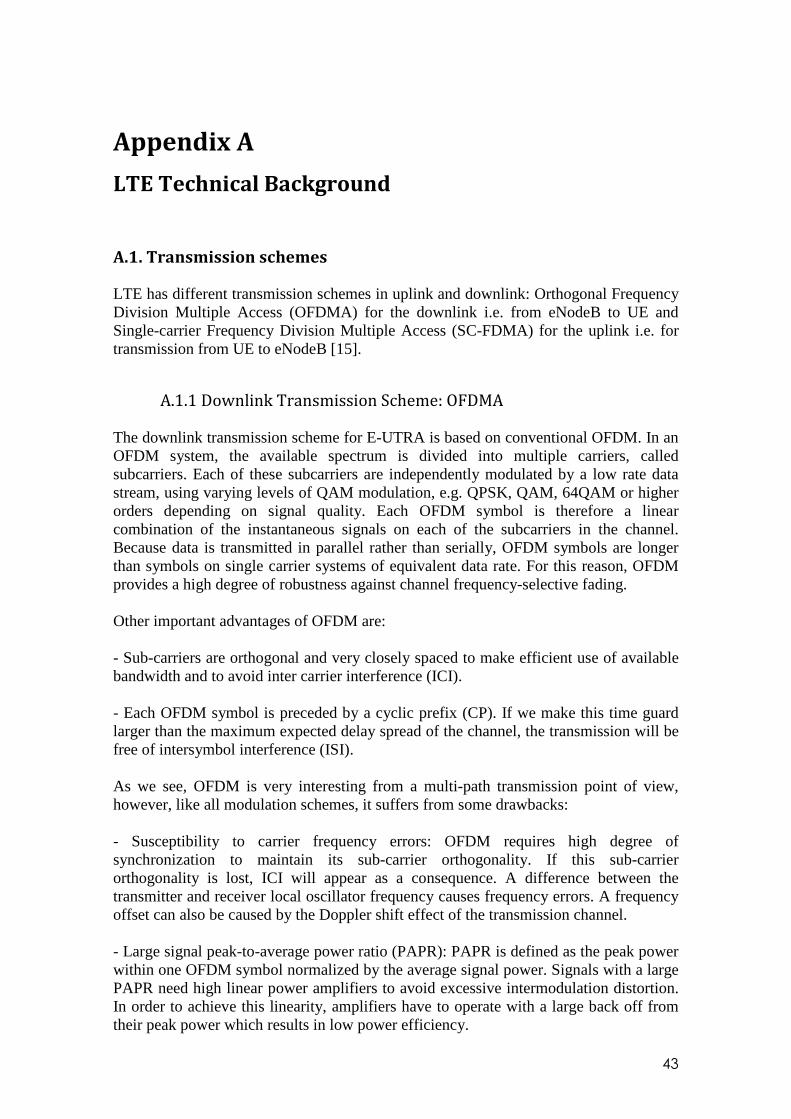
43

Appendix A

LTE Technical Background

A.1. Transmission schemes LTE has different transmission schemes in uplink and downlink: Orthogonal Frequency Division Multiple Access (OFDMA) for the downlink i.e. from eNodeB to UE and Single-carrier Frequency Division Multiple Access (SC-FDMA) for the uplink i.e. for transmission from UE to eNodeB [15].

A.1.1 Downlink Transmission Scheme: OFDMA The downlink transmission scheme for E-UTRA is based on conventional OFDM. In an OFDM system, the available spectrum is divided into multiple carriers, called subcarriers. Each of these subcarriers are independently modulated by a low rate data stream, using varying levels of QAM modulation, e.g. QPSK, QAM, 64QAM or higher orders depending on signal quality. Each OFDM symbol is therefore a linear combination of the instantaneous signals on each of the subcarriers in the channel. Because data is transmitted in parallel rather than serially, OFDM symbols are longer than symbols on single carrier systems of equivalent data rate. For this reason, OFDM provides a high degree of robustness against channel frequency-selective fading. Other important advantages of OFDM are: - Sub-carriers are orthogonal and very closely spaced to make efficient use of available bandwidth and to avoid inter carrier interference (ICI). - Each OFDM symbol is preceded by a cyclic prefix (CP). If we make this time guard larger than the maximum expected delay spread of the channel, the transmission will be free of intersymbol interference (ISI). As we see, OFDM is very interesting from a multi-path transmission point of view, however, like all modulation schemes, it suffers from some drawbacks: - Susceptibility to carrier frequency errors: OFDM requires high degree of synchronization to maintain its sub-carrier orthogonality. If this sub-carrier orthogonality is lost, ICI will appear as a consequence. A difference between the transmitter and receiver local oscillator frequency causes frequency errors. A frequency offset can also be caused by the Doppler shift effect of the transmission channel. - Large signal peak-to-average power ratio (PAPR): PAPR is defined as the peak power within one OFDM symbol normalized by the average signal power. Signals with a large PAPR need high linear power amplifiers to avoid excessive intermodulation distortion. In order to achieve this linearity, amplifiers have to operate with a large back off from their peak power which results in low power efficiency.

44

OFDMA is employed as the multiplexing scheme in the LTE downlink. In OFDMA, users are allocated a specific number of subcarriers for a predetermined amount of time. The samples of the transmitted OFDM signal can be obtained by performing an IFFT operation on the group of data symbols to be sent on orthogonal subcarriers. Similarly, the recovery of data symbols from the orthogonal subcarriers is accomplished using a FFT operation on a block of received samples. An illustrative description of a basic OFDMA transmitter/receiver is provided in Figure 24.

Figure 24. Transmitter and receiver structure of OFDMA system [15]

A.1.2 Uplink Transmission Scheme: SC-FDMA

Power consumption is a key consideration for mobile terminals. The high PAPR of an OFDM signal and the related high power consumption are major concerns. As a result, an alternative to OFDM has been selected for the LTE uplink transmission. Single Carrier Frequency Domain Multiple Access (SC-FDMA) is well suited to the LTE uplink requirements. The PAPR is low because the generated waveform is single carrier: SC-FDMA transmits on subcarriers in sequence not in parallel, so variations in the instantaneous transmit power are lower. The basic transmitter and receiver architecture is very similar to OFDMA, and it offers the same degree of multipath protection. An illustrative description of a basic SC-FDMA transmitter/receiver is provided in Figure 25.

Figure 25. Transmitter and receiver structure of SC-FDMA system [15]

45

A.1.3 OFDMA/SC-FDMA Signal generation As we have seen in the two figures above, the main blocks in an ODFMA and SC-FDMA chain transmission are the same. We make a more detailed analysis with the help of Figure 26, describing each one of the blocks. In the figure we can see the elements that are only present in SC-FDMA system or in both of them.

Figure 26. SC-FDMA and OFDMA Signal Chains [16]

Only chain transmission blocks are commented. In reception, they do the same function but in inverse way.

• SC-FDMA only: - Constellation mapper: It converts the bit stream to transmit to single carrier modulated symbols. - Serial/parallel converter: It formats time domain SC symbols into blocks for FFT input. - M-point DFT : It converts a time domain SC symbol block into M discrete tones.

• Both SC-FDMA and OFDMA: -cSubcarrier mapping: Maps DFT output tones to specified subcarriers for transmission. SC-FDMA LTE system use contiguous tones. - N-point IDFT : Converts mapped subcarriers back into time domain for transmission. - Cyclic prefix and pulse shaping: Cyclic prefix is pre-pended to the composite SC-FDMA/OFDM symbol to provide multipath immunity. Pulse shaping is employed to reduce out-of-band energy. - RFE: Converts digital signal to analog and convert to RF for channel transmission.

46

A.2 LTE Physical Layer

A.2.1 Frame Structure Two frame structures are defined for E-UTRA: frame structure type 1 for FDD mode, and frame structure type 2 for TDD mode. We work on FDD mode, so frame structure type 2 is discarded in this study. For FDD mode, a 10 ms radio frame structure is defined, which is divided into 20 equally sized slots of 0.5 ms. A subframe consists of two consecutive slots, so one radio frame contains ten subframes (Figure 27).

Figure 27. Frame structure type 1 [4]

Slots consist of either 6 or 7 OFDM symbols, depending on whether the normal or extended cyclic prefix is employed. Extended cyclic prefix is used in specific environments with very extensive delay spread, for example in very large cells, or in case of MBSFN-based multicast/broadcast transmission. In this entire study, we use normal cyclic prefix. Thus, we have 7 OFDM symbols per slot. In FDD, within one carrier, all the subframes of a frame are either used for downlink transmission or for uplink transmission (Figure 28).

Figure 28. Downlink/uplink subframe assignment in FDD case [5]

47

A.2.2 Physical Resource Transmitted signal in each slot is described by a resource grid of sub-carriers and available OFDM symbols. Each element in the resource grid is called a resource element and corresponds to one complex-valued modulation symbol. Each resource element corresponds to one OFDM subcarrier during one OFDM symbol interval. In both downlink and uplink, a basic scheduling unit is denoted a resource block. A resource block is defined as 7 consecutive OFDM symbols in the time domain (normal cyclic prefix) and 12 consecutive sub-carriers (180 kHz) in the frequency domain. Each sub-carrier spans 15 KHz (Figure 29).

Figure 29. Time-frequency grid [5]

The total number of subcarriers on a downlink carrier is Nsc =12·NRB +1, where NRB is the number of resource blocks, and the additional subcarrier is an unused DC-subcarrier,

which is allocated in the center of the downlink spectrum. The reason why the DC-subcarrier is not used for any transmission is that it may coincide with the local-oscillator frequency at the base-station transmitter and/or mobile-terminal receiver and cause high interference. The total number of subcarriers on an uplink carrier is Nsc =12·NRB. No unused DC-subcarrier is defined for the uplink, because the presence of a DC-carrier in the center of the spectrum will make it impossible to allocate the entire system bandwidth to a single mobile terminal and keep the low-PAR single-carrier property. Anyway, thanks to the DFT, the impact of any DC interference will be spread over the block of M modulation symbols and will be less harmful compared to normal OFDM transmission. LTE physical-layer specification actually allows for a downlink/uplink carrier to consist of any number of resource blocks, ranging from 6 resource blocks (1.4 MHz) up to 100 resource blocks (20 MHz).

48

A.2.3 Operating bands E-UTRA is designed to operate in 23 different operating bands, defined in LTE specifications [17]. In FDD mode, one band is defined for downlink and another for uplink, with a frequency separation which depends on the band. We work in E-UTRA Operating Band n° 7, where UL operating band is 2500 MHz –2570 MHz and DL operating band is 2620 MHz–2690 MHz. For this configuration, allowed channel bandwidths are 5 MHz, 10 MHz, 15 MHz and 20 MHz. [17] The channel raster in LTE is 100 kHz, which means that the carrier centre frequency must be an integer multiple of 100 kHz.

A.2.4 Channel structure LTE air interface consists of two main components:

• Physical signals, which are generated in Layer 1 and are used for system synchronization, cell identification and radio channel estimation. They are:

For the downlink: – Reference signal (RS) – Primary Synchronization signal – Secondary Synchronization signal For the uplink: – Reference signal (RS)

• Physical channels, which carry data from higher layers including control, scheduling and user payload. They are:

For the downlink: – Physical Broadcast Channel (PBCH) – Physical Control Format Indicator Channel (PCFICH) – Physical Downlink Control Channel (PDCCH) – Physical Hybrid ARQ Indicator Channel (PHICH) – Physical Downlink Shared Channel (PDSCH) – Physical Multicast Channel (PMCH) For the uplink: – Physical Uplink Shared Channel (PUSCH) – Physical Uplink Control Channel (PUCCH) – Physical Random Access Channel (PRACH)

49

Appendix B

Primary Synchronization sequences

B.1. Zadoff-Chu sequences properties Primary Synchronization signals are generated from Zadoff-Chu sequences. A Zadoff-Chu sequence is a complex-valued sequence given by:

))1(

exp()(ZC

u N

nunjnx

+−= π (9)

where NZC is the length of the sequence and 0≤n≤ NZC-1 The main properties of Zadoff-Chu sequences are: - Constant amplitude zero auto-correlation (CAZAC): The sequence modulus is one and its cyclic autocorrelation is zero. - Large peak to side-lobe ratio (PSR - ratio between the peak to the side-lobes of the aperiodic autocorrelation function): It allows the robust detection of the symbol timing at the terminal via simple time domain processing. - Low PAPR (peak-to-average power ratio): It improves the performance of the power amplifier and the coverage of the transmitted signal. - Cyclically shifted versions of the sequence do not cross-correlate with each other. A generated Zadoff–Chu sequence that has not been shifted is known as a “root sequence”. This property can be formulated as:

(10)

where rk (τ) is the cyclic autocorrelation function of ak at lag τ. The demonstration can be found in [18] - The cyclic cross-correlation between two Zadoff-Chu sequences of indices q1 and q2 is

constant and equal to 1/ ZCN if the difference |q1-q2| is relatively prime with respect to

the length of the sequence NZC. [19] - The DFT of a Zadoff-Chu sequence xu(n) is a Zadoff-Chu sequence Xw(k) such that w= -1/u mod NZC. It means that a Zadoff-Chu sequence can be generated directly in the frequency domain. [19]

∑−

=

=+=1

0

)()][(*)()(Nzc

nkkk nanar σδττ

50

B.1. P-SS correlation properties In LTE, Zadoff-Chu sequences have been chosen for the Primary Synchronization Signal. P-SS is a frequency-domain Zadoff-Chu sequence of length 63 with the middle element punctured to avoid transmitting on DC subcarrier. Three sequences are used of roots u=25, 29 and 34. Sequences are generated according to:

(1)

where dµ(n) denotes the P-SS, n denotes the subcarrier index where each sequence complex-symbol is mapped (P-SS it is transmitted on 62 out of the reserved 72 subcarriers around DC subcarrier) and µ denotes the sequence root index (25, 29 or 34). The puncturing on the symbol corresponding to DC subcarrier highly degrades the cylic correlation properties, but the aperiodic correlation properties remain almost the same. The set of roots for the P-SS has been chosen mainly for its low-frequency offset sensitivity (ratio of the maximum undesired autocorrelation peak in the time domain to the desired correlation peak computed at a certain frequency offset). This facilitates the P-SS detection during the initial synchronization. Moreover, sequences with root 29 and 34 are complex conjugates of each other and can be detected with a single correlator, so the receiver complexity is reduced. In Figure 30 and Figure 31 we compare the aperiodic correlation and cross-correlation of the chosen P-SS sequences. In Figure 31, we see that the cross-correlation between the pair of sequences with roots 25-34 is significantly worse than the others. The reason is that the difference between the roots, that is 9, is not relatively prime to the sequence length (Nzc=63), so the cyclic cross-correlation is not constant and the aperiodic cross-correlation is degraded as a consequence.

-60 -40 -20 0 20 40 600

0.2

0.4

0.6

0.8

1

Time shift (lag)

Cor

rela

tion

root 25

root 29&34


SS sequence as a function of time shift

-60 -40 -20 0 20 40 600

0.2

0.4

0.6

0.8

1

Time shift (lag)

Cor

rela

tion

roots 25-29

roots 29-34roots 25-34

Figure 31. Normalized cross-correlation function of a

P-SS sequence as a function of time shift

51

Appendix C

Secondary Synchronization sequences

C.1. S-SS generation Secondary Synchronization sequences are generated by the interleaved concatenation of two length-31 binary sequences in the frequency-domain (SCC1, SCC2). These two binary sequences are generated from the sequences s0(n) and s1(n), which are defined as two different cyclic shifts of a single M-sequence. These cyclic shifts, m0 and m1 respectively, are unique for each physical-layer cell-identity group (range from 0 to 167). Sequences s0(n) and s1(n) are next scrambled with the sequences c0(n) and c1(n), which are cyclic shifted versions of a length-31 binary sequence, where the shift value depends on the physical-layer identity (range from 0 to 2). Finally, there is a scrambling operation with the sequences z1

m0(n) and z0m1(n), which

are cyclic shifted-versions of the M-sequence z(n). S-SS differs from slot 0 to slot 10 in order to enable detection of radio frame timing. The generation of the S-SS is described Figure 32. All the expressions to generate the sequences are found in [4]

Figure 32. S-SS generation [6]

52

B.1. P-SS correlation properties S-SS have a flat frequency-domain correlation as shown in Figure 33 and Figure 34. In Figure 35 and Figure 36 we see the cross-correlation properties of the sequences. S-SS cross-correlation is degraded by the scrambling operations and depends on the considered pair of sequences.

-3 -2 -1 0 1 2

x 104

0

0.1

0.2

0.3

0.4

0.5

0.6

0.7

0.8

0.9

1

Frequency offset(Hz)

Aut

ocor

rela

tion

Figure 33. Normalized autocorrelation function of a S-

SS sequence as a function of frequency offset (cell

id=95, slot 0)

-3 -2 -1 0 1 2

x 104

0

0.1

0.2

0.3

0.4

0.5

0.6

0.7

0.8

0.9

1

Frequency offset(Hz)

Aut

ocor

rela

tion

Figure 34. Normalized autocorrelation function of a S-

SS sequence as a function of frequency offset (cell

id=57, slot 10)

0 20 40 60 80 100 120 140 1600

0.1

0.2

0.3

0.4

0.5

0.6

0.7

0.8

0.9

1

sequence index

Cor

rela

tion


S-SS sequence as a function of S-SS index (cell id=95,

slot 0)

0 20 40 60 80 100 120 140 1600

0.1

0.2

0.3

0.4

0.5

0.6

0.7

0.8

0.9

1

sequence index

Cor

rela

tion


S-SS sequence as a function of S-SS index (cell id =57,

slot 10)

53

Appendix D

Linear receivers

D.1. Matched Filter Matched filter correlates a received signal with a pattern signal in order to detect the presence of the pattern in the received signal. Matched filter is commonly used in the detection of deterministic signals, e.g. in radar applications. The matched filter is the optimal filter that maximizes the output SNR in the presence of additive white Gaussian noise, as it is shown in [20] Its expression is:

∑∞

−∞=

−=k

krknhny ][][][ (11)

where h[n] is the conjugated time-reversed version of the pattern signal p[n], with a and ∆ arbitrary constants: ][][ npanh H −∆⋅= (12) From the equation (12) and considering a given time instant: rhy H= (13)

D.2. Decorrelator The decorrelator has the same principle of the matched filter, but it has the particularity to reject the multiple access interference (MAI) [21]. It correlates the received signal with a set of orthonormal vectors which are the columns of the matrix F: 1)( −= SSSF H (14) where F is the pattern matrix, where each column represents a pattern sequence and FH is its conjugate transpose. The filtering is performed as in matched filter case, but with the columns “f” of the matrix F:

∑∞

−∞=

−=k

krknfny ][][][ (15)

We can define a column vector Y which represents all the decorrelator outputs for a given time instant: rFY H= (16) This structure leads to optimal decisions if and only if the pattern sequences are orthogonal. Unless, the noise components of the decorrelator outputs y are correlated and the detection decisions are not optimal as a consequence

54

(Demonstration)

We expand the equation (16): wFxFwxFrFy HHHH +=+⋅== )(

The covariance of the noise component wF H of the decorrelator output is [9]:

12 )( −= FFC Hy σ

So the noise components of the decorrelator outputs are decorrelated if and only if the pattern sequences are orthogonal (FHF=I ) A proposed solution in [9] consists in including a whitening filter H prior to the detection thresholds. The filter H is designed in order to obtain an equivalent structure “decorrelator+filter” which minimizes the least-square distance with the pattern signals. Then the structure exploits the multiple access interference (MAI) present in the received signal and the noise is optimally compensated. The optimal whitening filter structure has been solved in [22]: 2/1)( SSW H= (17) If we combine the decorrelator and the whitening filter we obtain: 2/12/11 )()()( −− === SSSSSSSSFWV HHHH (18)

55

Appendix E

Channel model In any wireless communication system, a signal which is exchanged between the transmitter and receiver antennas experiences the effects of the radio propagation channel. We can differentiate three main components: the path loss, the shadowing loss and the multipath fading.

E.1 Path loss Path loss is the power attenuation that suffers a signal due to the distance between the transmitter and the receiver:

β

φθd

)·C,·G(PT=RP (19)

where PR denotes the received signal power after path loss, PT is the transmit power, G( φθ , ) is the product of transmit-receive antenna gains which depends on the transmission-reception angle, β is the path loss coefficient and C is a constant that regroups the effect of other system parameters such as the antenna heights, the terrain type, etc. [23]

E.2 Shadowing Empirical measurements have shown that the variation of path loss around its mean follows a log-normal distribution (Gaussian if magnitude is measured in dB) with zero-mean and a standard deviation σ which depends on the environment (typically 8-10 dB in urban areas [24]). This variation, also called large-scale fading, is caused from shadowing effects of prominent obstacles in the propagation path between the mobile and the base station. In order to define a realistic shadowing model we take into account that time adjacent shadowing values are correlated depending on the velocity of the mobile. The normalized autocorrelation function follows an exponential function:

)2ln(

)( dcorr

x

exR∆

−=∆ (20)

where dcorr is the decorrelation length, ∆x represents the spatial distance considered between the time adjacent shadowing values. This model is described in [24]. Furthermore, if we consider multiple mobile-eNodeB links, the shadowing components affecting each one of the links have also a spatial correlation. A cross-correlation model is studied in [25].

200

9.0)(θθρ −= (21)

where θ is the angle formed by the two considered links. We integrate in our simulator both shadowing correlation models with the method proposed in [26].

56

E.3 Multipath fading Small-scale fading represents the fast variation in both signal amplitude and phase resulting from small changes in the spatial separation between the transmitter and the receiver. Many studies have proposed different distributions to characterize the envelope of the received signal. Main models are Rayleigh, Rician, Nakagami, etc. [23] We consider Rayleigh fading, which is appropriate for a channel model defined by multiple reflective paths with no line-of-sight dominant signal component. The methodology we use to simulate Rayleigh fading is described in [11] and is already implemented in Matlab. It is based on the “Jakes” Doppler spectrum model which is given analytically by:

2)/(1

1)(

dd

jfff

fS−⋅⋅

=π

dff ≤ (22)

where fd is the maximum Doppler Shift. Delay Spread In the simulations we consider different standard LTE environments. A complete definition of the tap delays and their power average attenuation for each LTE environment can be found in [12]. We only present the main parameters:

LTE environment R.M.S Delay spread Maximum Doppler Shift Extended Pedestrian Model 33.7 ns 5 Hz Extended Vehicular Model 83.7 ns 70 Hz

Extended Typical Urban Model 593.4 ns 300 Hz

57

Appendix F

3GPP LTE specifications

TS 36.101 Evolved Universal Terrestrial Radio Access (E-UTRA); User Equipment (UE) radio transmission and reception

TS 36.104 Evolved Universal Terrestrial Radio Access (E-UTRA); Base Station (BS) radio transmission and reception

TS 36.106 Evolved Universal Terrestrial Radio Access (E-UTRA); FDD repeater radio transmission and reception

TS 36.113 Evolved Universal Terrestrial Radio Access (E-UTRA); Base Station (BS) and repeater ElectroMagnetic Compatibility (EMC)

TS 36.124 Evolved Universal Terrestrial Radio Access (E-UTRA); Electromagnetic compatibility (EMC) requirements for mobile terminals and ancillary equipment

TS 36.133 Evolved Universal Terrestrial Radio Access (E-UTRA); Requirements for support of radio resource management

TS 36.141 Evolved Universal Terrestrial Radio Access (E-UTRA); Base Station (BS) conformance testing

TS 36.143 Evolved Universal Terrestrial Radio Access (E-UTRA); FDD epeater conformance testing

TS 36.201 Evolved Universal Terrestrial Radio Access (E-UTRA); Long Term Evolution (LTE) physical layer; General description

TS 36.211 Evolved Universal Terrestrial Radio Access (E-UTRA); Physical channels and modulation

TS 36.212 Evolved Universal Terrestrial Radio Access (E-UTRA); Multiplexing and channel coding

TS 36.213 Evolved Universal Terrestrial Radio Access (E-UTRA); Physical layer procedures

TS 36.214 Evolved Universal Terrestrial Radio Access (E-UTRA); Physical layer - Measurements

TS 36.300 Evolved Universal Terrestrial Radio Access (E-UTRA) and Evolved Universal Terrestrial Radio Access Network (E-UTRAN); Overall description; Stage 2

TS 36.302 Evolved Universal Terrestrial Radio Access (E-UTRA); Services provided by the physical layer

TS 36.304 Evolved Universal Terrestrial Radio Access (E-UTRA); User Equipment (UE) procedures in idle mode

TS 36.305 Evolved Universal Terrestrial Radio Access Network (E-UTRAN); Stage 2 functional specification of User Equipment (UE) positioning in E-UTRAN

TS 36.306 Evolved Universal Terrestrial Radio Access (E-UTRA); User Equipment (UE) radio access capabilities

TS 36.314 Evolved Universal Terrestrial Radio Access Network (E-UTRAN); Layer 2 - Measurements

TS 36.321 Evolved Universal Terrestrial Radio Access (E-UTRA); Medium Access Control (MAC) protocol specification

TS 36.322 Evolved Universal Terrestrial Radio Access (E-UTRA); Radio Link Control (RLC) protocol specification

TS 36.323 Evolved Universal Terrestrial Radio Access (E-UTRA); Packet Data Convergence Protocol (PDCP) specification

TS 36.331 Evolved Universal Terrestrial Radio Access (E-UTRA); Radio Resource Control (RRC); Protocol specification

TS 36.401 Evolved Universal Terrestrial Radio Access Network (E-UTRAN); Architecture description

TS 36.410 Evolved Universal Terrestrial Radio Access Network (E-UTRAN); S1 layer 1 general aspects and principles

TS 36.411 Evolved Universal Terrestrial Radio Access Network (E-UTRAN); S1 layer 1

TS 36.412 Evolved Universal Terrestrial Radio Access Network (E-UTRAN); S1 signalling transport

TS 36.413 Evolved Universal Terrestrial Radio Access (E-UTRA) ; S1 Application Protocol (S1AP)

TS 36.414 Evolved Universal Terrestrial Radio Access Network (E-UTRAN); S1 data transport

TS 36.420 Evolved Universal Terrestrial Radio Access Network (E-UTRAN); X2 general aspects and principles

TS 36.421 Evolved Universal Terrestrial Radio Access Network (E-UTRAN); X2 layer 1

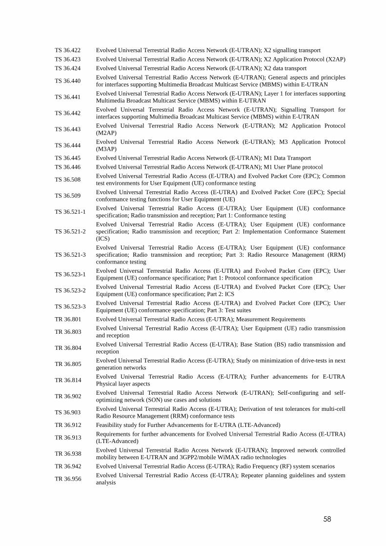
58

TS 36.422 Evolved Universal Terrestrial Radio Access Network (E-UTRAN); X2 signalling transport

TS 36.423 Evolved Universal Terrestrial Radio Access Network (E-UTRAN); X2 Application Protocol (X2AP)

TS 36.424 Evolved Universal Terrestrial Radio Access Network (E-UTRAN); X2 data transport

TS 36.440 Evolved Universal Terrestrial Radio Access Network (E-UTRAN); General aspects and principles for interfaces supporting Multimedia Broadcast Multicast Service (MBMS) within E-UTRAN

TS 36.441 Evolved Universal Terrestrial Radio Access Network (E-UTRAN); Layer 1 for interfaces supporting Multimedia Broadcast Multicast Service (MBMS) within E-UTRAN

TS 36.442 Evolved Universal Terrestrial Radio Access Network (E-UTRAN); Signalling Transport for interfaces supporting Multimedia Broadcast Multicast Service (MBMS) within E-UTRAN

TS 36.443 Evolved Universal Terrestrial Radio Access Network (E-UTRAN); M2 Application Protocol (M2AP)

TS 36.444 Evolved Universal Terrestrial Radio Access Network (E-UTRAN); M3 Application Protocol (M3AP)

TS 36.445 Evolved Universal Terrestrial Radio Access Network (E-UTRAN); M1 Data Transport

TS 36.446 Evolved Universal Terrestrial Radio Access Network (E-UTRAN); M1 User Plane protocol

TS 36.508 Evolved Universal Terrestrial Radio Access (E-UTRA) and Evolved Packet Core (EPC); Common test environments for User Equipment (UE) conformance testing

TS 36.509 Evolved Universal Terrestrial Radio Access (E-UTRA) and Evolved Packet Core (EPC); Special conformance testing functions for User Equipment (UE)

TS 36.521-1 Evolved Universal Terrestrial Radio Access (E-UTRA); User Equipment (UE) conformance specification; Radio transmission and reception; Part 1: Conformance testing

TS 36.521-2 Evolved Universal Terrestrial Radio Access (E-UTRA); User Equipment (UE) conformance specification; Radio transmission and reception; Part 2: Implementation Conformance Statement (ICS)

TS 36.521-3 Evolved Universal Terrestrial Radio Access (E-UTRA); User Equipment (UE) conformance specification; Radio transmission and reception; Part 3: Radio Resource Management (RRM) conformance testing

TS 36.523-1 Evolved Universal Terrestrial Radio Access (E-UTRA) and Evolved Packet Core (EPC); User Equipment (UE) conformance specification; Part 1: Protocol conformance specification

TS 36.523-2 Evolved Universal Terrestrial Radio Access (E-UTRA) and Evolved Packet Core (EPC); User Equipment (UE) conformance specification; Part 2: ICS

TS 36.523-3 Evolved Universal Terrestrial Radio Access (E-UTRA) and Evolved Packet Core (EPC); User Equipment (UE) conformance specification; Part 3: Test suites

TR 36.801 Evolved Universal Terrestrial Radio Access (E-UTRA); Measurement Requirements

TR 36.803 Evolved Universal Terrestrial Radio Access (E-UTRA); User Equipment (UE) radio transmission and reception

TR 36.804 Evolved Universal Terrestrial Radio Access (E-UTRA); Base Station (BS) radio transmission and reception

TR 36.805 Evolved Universal Terrestrial Radio Access (E-UTRA); Study on minimization of drive-tests in next generation networks

TR 36.814 Evolved Universal Terrestrial Radio Access (E-UTRA); Further advancements for E-UTRA Physical layer aspects

TR 36.902 Evolved Universal Terrestrial Radio Access Network (E-UTRAN); Self-configuring and self-optimizing network (SON) use cases and solutions

TS 36.903 Evolved Universal Terrestrial Radio Access (E-UTRA); Derivation of test tolerances for multi-cell Radio Resource Management (RRM) conformance tests

TR 36.912 Feasibility study for Further Advancements for E-UTRA (LTE-Advanced)

TR 36.913 Requirements for further advancements for Evolved Universal Terrestrial Radio Access (E-UTRA) (LTE-Advanced)

TR 36.938 Evolved Universal Terrestrial Radio Access Network (E-UTRAN); Improved network controlled mobility between E-UTRAN and 3GPP2/mobile WiMAX radio technologies

TR 36.942 Evolved Universal Terrestrial Radio Access (E-UTRA); Radio Frequency (RF) system scenarios

TR 36.956 Evolved Universal Terrestrial Radio Access (E-UTRA); Repeater planning guidelines and system analysis

Auto configuration dans LTE : procédés de mesure de · PDF fileAu cours de la...

Documents

Transcript of Auto configuration dans LTE : procédés de mesure de · PDF fileAu cours de la...