Author's personal copy - Shahab D....

This article appeared in a journal published by Elsevier. The attachedcopy is furnished to the author for internal non-commercial researchand education use, including for instruction at the authors institution

and sharing with colleagues.

Other uses, including reproduction and distribution, or selling orlicensing copies, or posting to personal, institutional or third party

websites are prohibited.

In most cases authors are permitted to post their version of thearticle (e.g. in Word or Tex form) to their personal website orinstitutional repository. Authors requiring further information

regarding Elsevier’s archiving and manuscript policies areencouraged to visit:

http://www.elsevier.com/copyright

http://www.elsevier.com/copyright

Author's personal copy

Intelligent seismic inversion workflow for high-resolution reservoircharacterization

E. Artun �,1, S. Mohaghegh

West Virginia University, Morgantown, W V, 26505, USA

a r t i c l e i n f o

Article history:

Received 26 June 2009

Received in revised form

24 May 2010

Accepted 26 May 2010Available online 10 August 2010

Keywords:

Seismic inversion

Neural networks

Reservoir characterization

Buffalo Valley Field

a b s t r a c t

Developing a geological model is the first and a very important step during the reservoir simulation and

modeling process. The geological model usually represents our best interpretation of the reservoir

characteristics that extends beyond the well where we have actual measurements (logs, core, well test,

etc.). The only real measurement with a large areal extent that geoscientists have access to is seismic

data. Therefore, using seismic data to populate the high-resolution geological model is becoming

increasingly popular. Using reservoir characteristics at the wellbore as the control point helps

geoscientists in measuring the goodness of the correlation they create between seismic data and well

logs. This paper presents a unique approach in accomplishing this task. The uniqueness of this approach

is based on the fact that (a) it reduces the complexity of the model building process by dividing a very

complex problem into two slightly less complex problems (surface seismic to VSP and VSP to log—i.e.,

divide and conquer) and (b) it effectively employs a synthetic set of formations representing the actual

sequence of geological layers in the field in order to build a model and learn from it, and then, apply the

lessons learned to the model building process for the actual reservoir. The results show that this

strategy proves to be successful.

& 2010 Elsevier Ltd. All rights reserved.

1. Introduction

The major challenge in today’s reservoir characterization is tointegrate all different kinds of data to attain an accurate and high-resolution reservoir model. Uncertainty, unreliability, and largevariety of scales due to the different origins of the data must betaken into consideration. These issues bring complex problems,which are hard to address with conventional tools. That is whyunconventional computation tools have gained much interest inrecent years. Among those modern tools; intelligent systems, as away of dealing with imprecision and partial truth, became awidely used method in reservoir characterization (Nikravesh andAminzadeh, 2001). Some previous intelligent reservoir character-ization applications include, but are not limited to, synthetic loggeneration (Mohaghegh et al., 1998, 2000; Rolon et al., 2009),permeability estimation from logs (Mohaghegh et al., 1994; Arpatet al., 1998), fracture frequency prediction (FitzGerald et al.,1999), lithology estimation (Walls et al., 1999) and predictingbulk volume of oil (Weiss et al., 2002). Poulton (2002) presented acomprehensive summary of neural-network applications ingeophysics.

Among the data used in reservoir characterization; coresamples provide very high-resolution information about thereservoir (fraction of inches), while seismic data have a resolutionin tens of feet, and well logs have in one of inches. Because of theirlow resolution, seismic data are routinely used only to attain astructural view of the reservoir. On the other hand, unlike coresamples or well logs, which are only available at isolated localitiesof a reservoir, seismic data frequently provide 3D coverage over alarge area and are incorporated into reservoir characterizationstudies. Inverse modeling of reservoir properties from seismicdata is known as seismic inversion in the literature. The workflowpresented in this paper includes inverse modeling of well logsfrom seismic data (surface seismic and vertical seismic profile)using intelligent systems (Fig. 1).

Seismic inversion has been applied in previous works withdifferent approaches. Multiple linear regression, back-propagationand probabilistic neural networks were used to predict porosity logs(Balch et al., 1999; Hampson et al., 2001; Leiphart and Hart, 2001;Dorrington and Link, 2004), gamma ray logs (Chawathe et al., 1997;Soto and Holditch, 1999), water saturation (Balch et al., 1999), net paythickness (Balch et al., 1999), sonic, density, and shale logs (Liu andLiu, 1998) from surface seismic attributes. Chawathe et al. (1997)have used higher-resolution cross-well seismic data instead of surfaceseismic as a new approach. Reeves et al. (2002) introduced a newmethodology, dividing the whole seismic inversion problem into two.They considered cross-well tomography as an intermediate step in

Contents lists available at ScienceDirect

journal homepage: www.elsevier.com/locate/cageo

Computers & Geosciences

0098-3004/$ - see front matter & 2010 Elsevier Ltd. All rights reserved.

doi:10.1016/j.cageo.2010.05.007

� Corresponding author.

E-mail address: [email protected] (E. Artun).1 Now with Chevron Energy Technology Company, Houston, Texas, USA.

Computers & Geosciences 37 (2011) 143–157


their procedure, after finding a correlation between surface seismicand cross-well seismic. They suggested producing virtual cross-wellseismic data and predicting logs from cross-well seismic attributes.They stated that using cross-well seismic as an intermediate scaledata can provide improved vertical resolution, increase constraintsand reduce the uncertainty of reservoir description.

In this study, vertical seismic profile (VSP) is incorporated into thestudy as the intermediate scale data. The intermediate step helps theneural network to solve a slightly less complex problem. Byperforming this step, we are providing the neural-network algorithmwith some help. It is a well known principle in the artificialintelligence (AI) practices to provide as much help in the form ofdomain expertise or incorporation of known functional analysis or inthis case an intermediate step that can increase the informationcontent of the data being provided to the neural-network algorithm.

VSP is known to be less expensive to obtain than cross-welltomography and to be available more frequently in oil fields. VSPdiffers from conventional seismic surveys in the location of signalreceivers. In VSP surveys, the receivers are located in the boreholeinstead of at the earth’s surface. Because the earth acts as a low-pass filter, placing of the receivers at depth reduces the distancethat the signal has to travel through the earth, thus yieldinghigher frequency (higher resolution) data (Gadallah, 1994).

The intelligent seismic inversion workflow proposed in thisstudy is shown in Fig. 2. The workflow starts with datapreparation by defining areal and vertical zones of interest first.Then, surface seismic/VSP attributes and well logs available

within the zones of interest are collected. A quality-check of thedata should be done and data must be arranged properly forneural network training.

Second part includes construction of neural-network basedcorrelation models. First, surface seismic-to-VSP models are trainedwith data from locations where both surface seismic and VSP areavailable. There would be a separate model for each VSP attribute.Second step is training of VSP-to-log models. This neural network istrained with data at locations where both VSP attributes and logs ofinterest are available. Third part is the prediction part. In this part ofthe workflow, correlation models trained in the second part are usedto predict VSP attributes and well logs. If we have reliable models, aVSP distribution map can be obtained for each attribute through thearea of interest. After obtaining the VSP distribution, that can beused to obtain estimated quantities of well logs by using the VSP-to-log models for each log.

The workflow is first applied to a synthetic model thatrepresents the gas-producing Atoka and Morrow formations andthe overlying Pennsylvanian sequence in the Buffalo Valley Fieldin New Mexico. In this way, we aimed to build a model, and learn

Fig. 1. Seismic inversion process: modeling high-frequency logs from low-

frequency seismic signals.

Data Preparation

Model Construction

Prediction

Step 1: Prediction of VSP attributes from surface seismic attributes(using surface seismic-to-VSP models trained in Step 1 of Model Construction)

Step 2: Prediction of well logs from VSP attributes(using VSP-to-log models trained in Step 2 of Model Construction)

Step 1: Neural network training for Surface seismic-to-VSP models- inputs: surface seismic attributes- outputs: VSP attributes

Step 2: Neural network training for VSP-to-log models- inputs: VSP attributes- outputs: well logs

Collecting surface seismic attributes, VSP attributes and well logs at areal and vertical zones of interest

Fig. 2. Proposed seismic inversion workflow to model high-frequency logs from low-frequency seismic signals.

Table 1Derived seismic attributes used in this study.

1. 1st derivative of seismic trace dr(t)/dt

2. 2nd derivative of seismic trace d2r(t)/dt2

3. 1st derivative of envelope de(t)/dt

4. 2nd derivative of envelope d2e(t)/dt2

5. Instantaneous energy E¼e2(t)

6. Instantaneous power dE/dt

7. Instantaneous acceleration aðtÞ ¼ do=dt

8. DecaydðtÞ ¼

deðtÞ=dt

eðtÞ9. Instantaneous quality factor qðtÞ ¼ poðtÞ=dðtÞ

10. Amplitude weighted phase ¼ eðtÞfðtÞ11. Average frequency

/oðtÞS¼Ptþk

t�k

oðtÞð2kþ1Þ

12. Residual envelopeeðtÞ�

Ptþkt�k

eðtÞ

ð2kþ1Þ

� �13. Integrated residual envelope P

t eðtÞ�Ptþk

t�k

eðtÞ

ð2kþ1Þ

� �� 14. Smoothed envelope

eSðtÞ ¼Ptþk

t�k

eðtÞ

ð2kþ1Þ

� �15. Integrated absolute amplitude IAðtÞ ¼

Pt0 eðtÞ�

Pt0 eSðtÞ

E. Artun, S. Mohaghegh / Computers & Geosciences 37 (2011) 143–157144


from it before applying the workflow to the actual reservoir. In thesynthetic case, density and acoustic velocity logs, which aresurrogates for reservoir porosity, were the only two types ofavailable logs. In the field case, seismic field data are used topredict gamma ray and neutron porosity distributions through aseismic section. A general regression neural network algorithm isused in neural network training. Multiple linear regression is alsoutilized as a conventional correlation scheme to compare with theproposed methodology. The principal objectives of this study canbe listed as the following:

1. developing an intelligent seismic inversion workflow tocorrelate seismic attributes to well logs;

2. assessing the usefulness of incorporating an intermediate stepby comparing the proposed workflow with a conventionalseismic-to-log correlation scheme;

3. assessing the usefulness of testing the workflow on a syntheticmodel before applying it to the actual reservoir;

4. identifying best practices and challenges in utilizing theproposed workflow.

Seismic attributes used in this study are calculated within atime window that represents the producing Atoka and Morrowformations of the Buffalo Valley Field. In addition to some majorattributes such as amplitude (r(t)), envelope (e(t)), frequency(oðtÞ), finite difference, average energy (E(t)), paraphase, phase(jðtÞ), peak-to-trough, Hilbert transform (h(t)¼ i(t)), and signedfrequency, attributes listed in Table 1 are also derived andincorporated into the field study. In the synthetic modeling study,amplitude, envelope, frequency, average energy, paraphase,phase, peak-to-trough, and Hilbert transform were available(Mohaghegh et al., 2005).

2. General regression neural network (GRNN) algorithm

GRNN is a one-pass learning algorithm with a highly parallelstructure (Specht, 1991). It is a memory-based network, which

provides estimates of continuous variables, and converges to theunderlying regression surface. This approach is freed fromthe necessity of assuming a specific functional form. Instead,the appropriate form is expressed as a probability density function

(PDF) which can be determined from the observed data. Generalregression uses y (a scalar random variable), the X (a particularmeasured value of a vector random variable x), and the non-parametric estimator of the joint p.d.f. f(x,y). After defining thescalar Euclidian distance function, Di

2;

D2i ¼ ðX�Xi

ÞTðX�Xi

Þ ð1Þ

performing the integrations results with the following:

Y ðXÞ ¼

Pni ¼ 1 Yiexp �

D2i

2s

!

Pni ¼ 1 exp �

D2i

2s

! ð2Þ

Table 2Layers and corresponding density and velocity ranges of synthetic model.

Lithology Density (g/cc) Velocity (m/s)

Sandstone 2.4–2.7 3810–4875

Shale 1.9–2.10 2745–3350

Limestone 2.5–2.7 4270–5180

Velocity (m/s)x (m)

Tim

e (s

ec)

1000 2000 3000 4000 5000 6000 70000.8

0.85

0.9

0.95

1

1.05

1.10.8

1

1.2

1.4

1.6

1.8

2

2.2

x 104

Fig. 3. Velocity response of synthetic model.

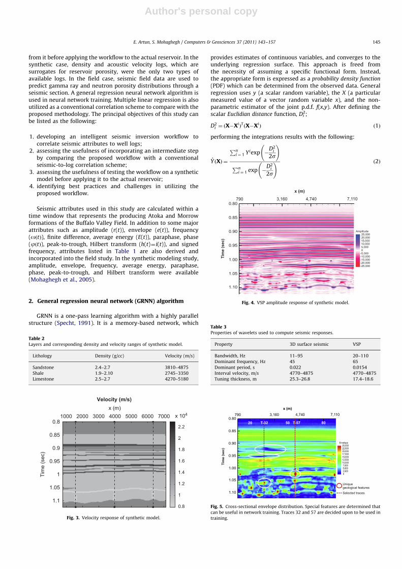
Fig. 5. Cross-sectional envelope distribution. Special features are determined that

can be useful in network training. Traces 32 and 57 are decided upon to be used in

training.

Table 3Properties of wavelets used to compute seismic responses.

Property 3D surface seismic VSP

Bandwidth, Hz 11–95 20–110

Dominant frequency, Hz 45 65

Dominant period, s 0.022 0.0154

Interval velocity, m/s 4770–4875 4770–4875

Tuning thickness, m 25.3–26.8 17.4–18.6

Fig. 4. VSP amplitude response of synthetic model.

E. Artun, S. Mohaghegh / Computers & Geosciences 37 (2011) 143–157 145


To define it in a simpler mathematical form, Eq. (4) is proposedinstead of (2), which has given similar results. Instead of theEuclidian distance, it uses the city block distance, Ci;

Ci ¼Xp

i ¼ 1

jðXj�XijÞj ð3Þ

Y ðXÞ ¼

Pni ¼ 1 Yiexp �

Ci

s

� �Pn

i ¼ 1 exp �Ci

s

� � ð4Þ

The estimate Y(X) is defined as a weighted average of the observedvalues, Yi, where each observed value is weighted exponentiallyaccording to its Euclidean or city block distance (Specht, 1991). sis the smoothing factor, and optimum smoothing factor isdetermined after several runs according to the mean-squarederror of the estimate, which must be kept at minimum. Thesmoothing factor must be greater than 0 and can usually rangefrom 0.01 to 1 with good results (Neuroshell, 1998). This processis named as the training of the network. If a number of iterationspasses with no improvement in the mean-squared error, thatsmoothing factor is determined as the optimum one for that dataset. In the verification phase, that smoothing factor is applied todata sets that the network has not seen before. While applying thenetwork to a new set of data, increasing the smoothing factorwould result with decreasing the range output values.

GRNN is a modification to probabilistic neural network thathas been suggested by authors, who have studied seismicinversion scale-down correlations (Hampson et al., 2001; Leiphartand Hart, 2001; Reeves et al., 2002; Luca, 2001). GRNN has alsobeen successfully used in geological pattern recognition applica-tions such as; synthetic log generation (Rolon et al., 2009) andtotal organic carbon content prediction from logs (Huang andWilliamson, 1994). Huang and Williamson (1994) describedGRNN as an easy-to-implement tool, which has efficient trainingcapabilities, and the ability to handle incomplete patterns. GRNNis known to be particularly useful in approximating continuousfunctions, such as logs, or other types of geological patterns. Itmay have multidimensional input, and it will fit multidimensionalsurfaces through data. It is a three-layer network. In the hiddenlayer, there must be one hidden neuron for each training pattern.In this study, Neuroshell 2TM software is used to train andconstruct GRNN-based correlation models.

3. Case 1: synthetic model study

3.1. Description of the model

The model used in this study was developed by Sanchez (2004)using StructTM (a modeling package in the Geographix DiscoverySuite of Landmark GraphicsTM). It is a comparative example of thestratigraphic section of the Buffalo Valley Field, which includesAtoka and Morrow formations together with the overlyingPennsylvanian sequence (0.8–1.124 s). It was developed by usinga forward modeling process, which has simulated straight raystraveling from the surface and avoiding diffraction at interferingevents. The model has a horizontal dimension of 7.9 km (4.9 mi),equivalent to the dimension of the 3D seismic survey at a depth of2134 m (7000 ft) thickness of the sequence was measured as610 m (2000 ft) from the well logs. Based on well log interpreta-tion and seismic visualization, thicknesses of sand channels andsandstone/limestone layers were in the range of 10 and 80 ft. Theaverage density and velocity of shales and sand bodies werederived from well logs and they are presented in Table 2 (Sanchez,2004).

Two separate models were obtained by extracting waveletsfrom actual surface seismic and VSP for the time window of theAtoka and Morrow formations. The velocity response of the modelis shown in Fig. 3 with the dashed lines representing three wellsat traces 20, 50 and 80. The synthetic surface seismic responsewas computed by using a wavelet derived from the zone ofinterest in line 1034 of the 3D surface seismic data, and thesynthetic VSP response (Fig. 4) was computed by using aButterworth wavelet derived from line 2064 of the 3D VSP witha larger bandwidth. The properties of the wavelets used for eachcase are presented in Table 3. Tuning thickness has beendetermined after the vertical resolution has been calculated withthe relationship

VR¼ v=4f ð5Þ

where VR is the vertical resolution in m/(s�Hz), v is the intervalvelocity in m/s and f is the dominant frequency in Hz. The 1%noise were introduced to the model during the computations(Sanchez, 2004).

The model is a seismic line of 100 traces, which includes threewells at traces 20, 50 and 80 with the well at trace-50 having aVSP survey. These wells had well logs of density and acoustic

Fig. 6. Network structures used for training. (a) Data of traces 32 and 57 have been

used, to predict a VSP attribute from time and surface seismic attributes. (b) Data

of Trace-50 have been used, to predict one of density classes from time and VSP

attributes.

Table 4Correlation coefficients for neural network models developed for synthetic model

study (first correlation step).

All Training Calibration Verification

Amplitude 1.00 1.00 1.00 1.00

A. energy 0.91 0.92 0.89 0.86

Envelope 0.98 0.99 0.95 0.95

Frequency 0.87 0.87 0.90 0.86

Hilbert T. 0.96 0.95 0.95 0.98

Paraphase 0.94 0.94 0.92 0.92

Phase 0.96 0.99 1.00 0.72



velocity. The data used are within the interval 0.8–1.124 s(2012–2743 m; 6600–9000 ft), as it represents a majorexploration target in the area. Above this interval, there is seismicnoise that was ignored as input data. The available data that wereoutput from the model were;

1. Surface seismic and VSP responses in the form of the seismicattributes: amplitude, average energy, envelope, instantaneousfrequency, Hilbert transform, paraphrase, instantaneous phase.

2. Density and acoustic velocity distributions.

3.2. Utilization of the workflow

3.2.1. Step 1: correlation of surface seismic with VSP

An effort was made to find a correlation between surfaceseismic attributes and VSP attributes. First, the model wasvisualized with cross-sectional distributions of density, acousticvelocity, surface seismic and VSP attributes. It was aimed todetermine the most appropriate portion of the synthetic data setthat should be used in training of the network. The training data

set must be representative of the geological complexity of thearea being modeled. Only then, one can obtain successful resultsin the prediction stage. For this purpose, an effort was made toidentify unique geological features including edges of sandchannels, and extreme-value points. In this particular case, thosekinds of features could be found mostly in the central part of thesynthetic seismic section. We decided to use only traces 32 and 57to keep the number of traces at minimum (Fig. 5). The networkstructure used in training is shown in Fig. 6a. As shown, each VSPattribute was to be predicted from time and seven availablesurface seismic attributes. At the end, seven separate predictionmodels have been developed for seven attributes. After havingconfidence of the prediction abilities of these models, they wereapplied to the whole seismic line to obtain network-predicteddistributions of all the available seismic attributes from VSP.These attributes were then plotted in order to compare them withthe actual ones.

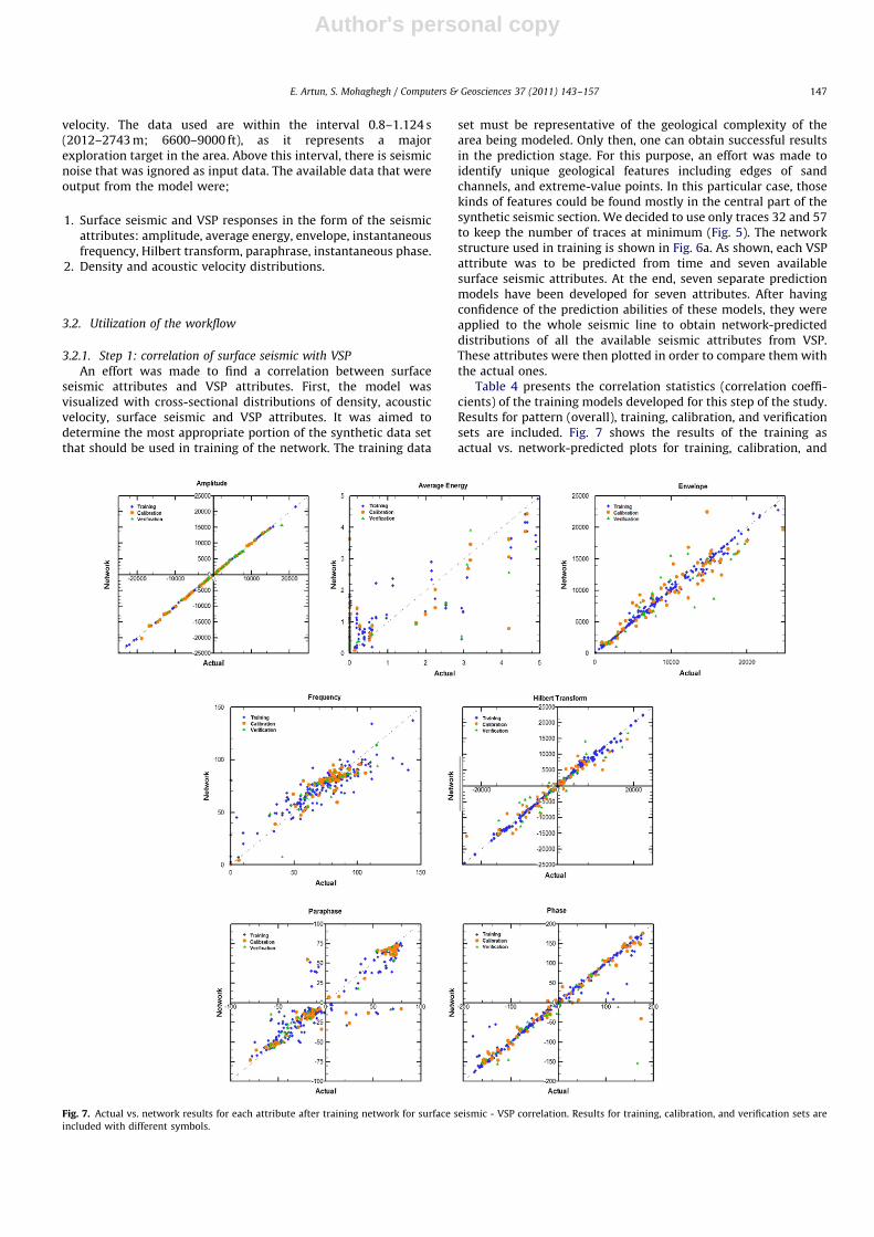
Table 4 presents the correlation statistics (correlation coeffi-cients) of the training models developed for this step of the study.Results for pattern (overall), training, calibration, and verificationsets are included. Fig. 7 shows the results of the training asactual vs. network-predicted plots for training, calibration, and

Fig. 7. Actual vs. network results for each attribute after training network for surface seismic - VSP correlation. Results for training, calibration, and verification sets are

included with different symbols.



verification sets of seven attributes. Each set of data is shown witha different symbol. Statistical and visual results indicate thatreliable models have been developed. These models have beenapplied to the whole line (i.e., other traces of the synthetic model).The seismic attribute distributions have been reproduced. Theyhave been re-plotted to be able to compare with the actualdistributions. Fig. 8 shows the comparison plots for three

attributes: amplitude, average energy, and envelope; and Fig. 9shows the plots for three other attributes: frequency, Hilberttransform, and paraphase, which are obtained after applying themodels for these attributes to the entire line. These plots alsoinclude the actual log lines of each attribute at traces 20, 35, 50,65, and, 80, which makes it easier to assess the quality of thenetwork-predicted distributions.

Fig. 8. Actual (left) and network-predicted (right) distributions for VSP attributes: amplitude, average energy, and envelope.



3.2.2. Step 2: correlation of VSP with well logs

The second step of the correlation was deriving log propertiesfrom the neural network-derived VSP data. Since trace 50 isthe trace which includes all of the data that we are dealing with(i.e., surface seismic, VSP and well logs), this trace was used todevelop the model for this part of the correlation. The density logwas selected as the target log. To simplify the problem, values ofthe density log were treated as different classes that represent a

different type of rock layer defined in the model. By doing this, wehave changed the nature of the neural modeling to one ofclassification. Classification networks are sometimes simpler thannetworks that are built to predict continuous values. In the initialtrial; classes were defined for density values of 1.9 g/cc (Class 1),2.3 g/cc (Class 2), 2.65 g/cc (Class 3).

The input/output structure of the neural network is shown inFig. 6b. All of the VSP attributes and time are used as inputs to

Fig. 9. Actual (left) and network-predicted (right) distributions for VSP attributes: frequency, Hilbert transform, and paraphase.



predict one of the density classes. For the density prediction, actualdensity log line and network predictions are shown in Fig. 10a.Although the network performed successfully in most parts, it hasmissed some points when the density is between 2.1 and 2.4 g/ccwhich were defined to belong to the class of r¼ 2:3 g=cc (Class 2).To overcome this problem, it was decided to introduce anotherclass to our model. Class 4 was assigned to density values around2.09 g/cc (Fig. 10b). That has helped the network to be successful inall ranges of values (Fig. 10b), and this network model was chosento be used in prediction. The correlation statistics of this model arepresented in Table 5 together with the results for the velocity log.Predicted VSP attributes from the first correlation step wereapplied to this model, and density log is predicted along theseismic line with a correlation coefficient of 0.81. Top twodistributions in Fig. 11 show the final actual vs. network-predicteddensity distributions, respectively. It is seen that, the lithologicalunits as well as the sand channels have been successfully predictedby the neural network.

3.3. Comparison with conventional seismic-to-log correlation

scheme

Multiple linear regression (MLR) is a widely known correlationmethod. To compare GRNN used in this study with a conventionalseismic-to-log correlation scheme, the workflow proposed isrepeated using MLR instead of GRNN by using surface seismic

Fig. 10. Defining density classes, and corresponding training results. (a) Three classes (1.9, 2.3, 2.65). r¼0.82 for training set, (b) Four classes (1.9, 2.09, 2.3, 2.65). r¼0.94

for training set.

Table 5Correlation coefficients for neural network models developed for synthetic model

study (second correlation step).


Density 0.91 0.97 0.73 0.73

Velocity 0.95 0.96 0.99 0.70



attributes as inputs and density log as the single output. Table 6presents the coefficients of input parameters (surface seismicattributes) obtained for this model. Fig. 12 shows the MLR-modelpredictions for trace-50 which is the well in the center of the

Actual Density (g/cc)x (m)

Tim

e (s

ec)

1000 70000.8

0.85

0.9

0.95

1

1.05

1.11.9

2

2.1

2.2

2.3

2.4

2.5

2.6

ANN−Predicted Density (g/cc), r = 0.81x (m)

Tim

e (s

ec)

1000 2000 3000 4000 5000 6000

2000 3000 4000 5000 6000

70000.8

0.85

0.9

0.95

1

1.05

1.11.9

2

2.1

2.2

2.3

2.4

2.5

2.6

MLR−Predicted Density (g/cc), r = 0.50x (m)

Tim

e (s

ec)

1000 2000 3000 4000 5000 6000 70000.8

0.85

0.9

0.95

1

1.05

1.11.9

2

2.1

2.2

2.3

2.4

2.5

2.6

Fig. 11. Actual, neural network and multiple linear regression predicted distribu-

tions of density values.

Table 6Multiple linear regression coefficients for input parameters.

Intercept 3.06304

Time �0.55609

Amplitude 0.00005

Average energy �0.13689

Envelope �0.00020

Frequency �0.00021

Hilbert transform 0.00004

Peak-to-trough 0.00009

Phase �0.00721

Paraphase �0.00054

0.8

0.85

0.9

0.95

1

1.05

1.1

1.7 1.9 2.1 2.3 2.5 2.7

Tim

e, s

ec

Density, g/cc

Density - Trace 50r = 0.52

ActualMLR

Fig. 12. Actual, and multiple linear regression predicted density log values in

trace-50.

Fig. 13. An illustration of logs having good and bad qualities.



synthetic model. It is seen that the predictions are not asaccurate as neural network (GRNN) predictions. In Fig. 11,density distribution along the synthetic seismic line predictedby MLR-model is shown. MLR-model was not able to

provide a similar level of accuracy as neural networkmodel did. The correlation coefficient with MLR is 0.50,which is significantly less than 0.81 obtained with the neuralnetwork.

Fig. 14. Left: map of wells available logs within seismic survey area of Buffalo Valley Field. Seismic line chosen to work with, and five wells on that line are highlighted.

Center: amplitude distribution of seismic line. Red dashed lines are five wells, line is passing through. Right: VSP amplitude profile of Well-1. (For interpretation of the

references to colour in this figure legend, the reader is referred to the web version of this article.)

Table 7Correlation coefficients for eleven VSP attributes (first correlation step of the real case study).


Amplitude 0.98 1.00 0.95 0.95

A. energy 0.98 0.99 0.99 0.92

Envelope 0.99 0.99 0.99 0.92

Finite diff. 0.96 0.99 0.99 0.91

Frequency 0.58 0.99 0.99 0.46

Hilbert T. 0.99 0.99 0.99 0.96

Inversion 0.99 0.99 0.99 0.99

Paraphase 0.89 0.89 0.95 0.54

Peak-to-trough ratio 0.96 0.99 0.95 0.89

Phase 0.80 0.98 0.86 0.64

Signed frequency 0.96 0.99 0.93 0.30

Fig. 15. Actual vs. network plots for inversion, phase, paraphase, peak-to-trough, and signed frequency shown as logs.



4. Case 2: field study (B. Valley Field, New Mexico)

The following seismic data were used in this study (Sanchez,2004):

1. A 3D seismic survey, loaned by Western Geco for this study,covering an area of 62 km2 (24 mi2) with a vibroseis source,sweep frequencies ranging from 8 to 98 Hz, and a sweep lengthof 17 s.

2. A vertical seismic profile volume, with a two-LRS-315vibrators source, covering an area of approximately 9 km2

(3.5 mi2) in the southeast corner of the area.

Unfortunately, not all of the available well logs were of high visualquality. That made them hard to accurately digitize. An illustra-tion for good quality logs and bad quality logs are shown inFig. 13. The quality of the data has an important role in buildingreliable neural network models. Reasonable amount of noise inthe data is acceptable, and even useful for a more realistic

Fig. 16. Actual vs. network plots for six attributes. Training, calibration, and verification sets are included with different symbols.



training. However, it is impossible to rely on a model, which hasbeen built with unreliable data. Rolon et al. (2009) clearly statesthis fact, by comparing two similar studies with well log data

having different levels of quality. Given these issues, digitized logfiles were evaluated by visual analysis. Well logs with goodoverall quality were selected for neural network design to avoidbuilding poor prediction models. Within the context of log qualityand distribution, and the location of the VSP well, a seismic line(Fig. 14) was extracted from the 3D survey area for use in theneural network design and evaluation. The line trends SE–NWthrough the survey area, and passes through five wells includingthe VSP well. The line included 173 seismic traces; the VSP well,Well-1, located on trace 16 (Fig. 14). Other wells are located ontraces 55, 90, 123, and 153, respectively. The data shown in Fig. 14are seismic amplitude distribution and VSP amplitude profile forWell-1. VSP data were available only for Well-1. Surface seismicdata used in the analysis extended from 0.92–1.10 s (two-waytime). This interval includes reflection events associated with theAtoka–Morrow target interval. A total of 26 seismic attributeswere available. Eleven of these attributes were provided by theKingdom Suite, and other 15 attributes were calculated usingtheoretical relationships (Table 1). Additional attributes includeda variety of derivatives, instantaneous energy, power andacceleration, quality factor, acoustic impedance inversions, andvarious residuals and smoothed outputs of other attributes(Mohaghegh et al., 2005).

4.1. Utilization of the workflow

The methodology as the one employed in the synthetic casestudy was followed in this case. Since there was only oneavailable VSP survey (Well-1), the required correlation models forVSP prediction were restricted to data from that well. The seismicattribute data were re-sampled to 0.0005 s (half-millisecond).Well log responses in depth were converted to time usingmodified well and surface seismic velocity functions. The logresponses were also re-sampled to half-millisecond intervals.

Surface seismic–VSP correlation models have been developed,by using time and eleven surface seismic attributes to predict thesingle VSP attribute. The attributes used in this study were theones which have been generated from the Kingdom Suite as theother attributes can be derived by using those ones. Table 7presents the correlation statistics for these models for eachattribute. Results for pattern, training, calibration, and verificationsets are included. Their actual vs. network graphs are shown inFig. 15. Actual vs. network plots for some other attributes are

Table 8Results of key performance indicators for gamma ray and neutron porosity.

Rank Gamma ray Neutron porosity

1 Peak-to-trough* Amp weighted phase*

2 Smoothed envelope* Time*

3 Finite difference* Peak-to-trough*

4 Average frequency* Instant energy*

5 Instant energy* Smoothed envelope*

6 Envelope* Envelope*

7 Time* Amplitude*

8 Amp weighted phase* HF inversion*

9 Amplitude* Finite difference

10 Phase* Average energy

11 Hilbert* Frequency

12 Smoothed inversion* Paraphase

13 HF inversion* Hilbert

14 1st D amp Smoothed inversion

15 Average energy Decay rate

16 Inst. accel Phase

17 Inst. Q fac Signed freq

18 Decay rate Frequency

19 2nd D amp 1st D amp

20 Res env Inst res env

Ones with ‘*’ superscript were used as inputs. Top 20 attributes are shown.

Table 9Correlation coefficients for pattern, training, and calibration sets of training model

for gamma ray and neutron porosity logs.

All Training Calibration

Gamma ray

All 0.88 0.89 0.77

Well-1 0.76 0.75 0.85

Well-2 0.86 0.87 0.82

Well-3 0.81 0.85 0.52

Well-4 0.90 0.88 0.52

Well-5 0.90 0.91 0.83

Neutron porosity

All 0.97 0.98 0.91

Well-1 0.98 0.98 0.88

Well-2 0.97 0.97 0.94

Fig. 17. Actual and network-predicted gamma ray logs for wells 1, 2, 3, 4, and 5. Values for training, and calibration sets are included. VSP attributes were used as inputs.



shown in Fig. 16. These results show that accurate correlations areobtained between surface seismic and VSP attributes. Thesemodels were then applied to other traces on the seismic line,with the available surface seismic data. VSP distributions wereproduced through the entire seismic line.

In the log prediction stage, the approach that has been carriedout was to use all the available well data for training, and to applythe model to other parts of the seismic line to obtain thedistributions. The main idea is to have a more reliable trainingmodel by using all the available data. In this case, 90% of the totalof 871 rows of data from five wells was used for training, while10% was used for testing. Two types of logs: gamma ray andneutron porosity were selected as target logs. Because of the largenumber of available attributes a key performance indicator (KPI)study was carried out, to determine the most influentialattributes. This was done using Intelligent Reservoir Character-ization Analysis software of Intelligent Solutions.1 As a result ofthis study each attribute had a coefficient between 0 and 1, whichbasically shows the influence of that attribute on the selectedoutput (i.e., logs). The attributes (including the time) were rankedbased on their KPI coefficients and the ones having a coefficientlarger than 0.5 were used as inputs. Those rankings for gamma rayand neutron porosity are presented in Table 8. The best thirteenattributes for the gamma ray, and the best eight attributes for theneutron porosity had coefficients higher than 0.5, and they wereused as the input attributes.

In the log prediction stage, gamma ray and neutron porosityare used as the target logs. Correlation statistics are presented inTable 9 for pattern, training, and testing sets, respectively. Resultsare showing both overall statistics, and individual well statistics.Graphs that show actual and network-predicted log lines for thegamma ray log are shown in Fig. 17 for all wells. Neutron porositylogs were available in only two wells; Well-1 and Well-2. Thus,these two wells were used in training. Fig. 18 shows the actual

and network-predicted logs for two wells for the neutron porositylog. Predicted distributions of gamma-ray and neutron porositylog along the seismic line are shown in Fig. 19. Actual log lines arealso shown in the plot which gives a better understanding of theaccuracy of these predictions. It is seen that predicted distribu-tions match with the actual well log lines quantitatively.

4.2. Comparison with conventional seismic-to-log correlation

scheme

The workflow is repeated with multiple linear regression(MLR) for the field study. Together with time, 10 surface seismicattributes with the highest ranking in Table 8 are used as inputsfor gamma ray and neutron porosity logs. Seperate MLR modelswere constructed for Well-1 and Well-2. However, correlationmodels did not provide accurate predictions even for the well thatthey are constructed with. The coefficients are presented inTable 10. Fig. 20 shows the gamma ray and neutron porosity logsfor Well-1 and Well-2 with the predictions of MLR-model. It isobserved that MLR-based models were not as successful as neuralnetwork-based correlation models.

5. Summary and conclusions

In this study, a new approach to the seismic inversion problemis introduced. A two-step, intelligent seismic inversion methodol-ogy is successfully implemented on a synthetic model, and real

Fig. 19. Network-predicted well log distributions through seismic line of interest:

(a) gamma ray log, (b) neutron porosity log. Actual log lines are also shown.

Fig. 18. Actual and network-predicted neutron porosity logs for wells 1, and 2.

Values for training, and calibration sets are included. VSP attributes were used as

inputs.

1 http://www.intelligentsolutionsinc.com



data of the Buffalo Valley Field, New Mexico. The main conclu-sions of this study can be summarized as follows:

1. The complex and non-linear relationship between seismicattributes and reservoir properties was extracted using artificialneural networks. General regression neural network (GRNN),which is a useful algorithm for approximating continuousfunctions, was applied successfully in this study.

2. It is beneficial to use a synthetic seismic model in developingthe appropriate methodology by identifying the most appro-priate neural network algorithm and testing the use of othertools. The synthetic model not only made it easy to be familiarwith the types of data that are dealt with, but also provided theopportunity of comparing results for the whole seismicsection. Although it was not applicable for the field study, aclassification (lithology identification) approach was used inthe synthetic model study.

3. Although there are several examples of using artificial neuralnetworks to correlate seismic attributes to reservoir proper-ties, or well logs, this study is unique because of integratingthree types and scales of data (surface seismic, VSP, and welllogs).

4. To determine the data that should be used for training, modelvisualization is beneficial. It was seen in the synthetic modelstudy that including diverse geological characteristics in thetraining set can increase the generalization abilities of neuralnetwork based predictors.

5. The workflow proposed in this study provided better predic-tions than a conventional seismic-to-log correlation schemewith multiple linear regression.

Acknowledgements

This research was supported by a Grant from the U.S. Departmentof Energy (DE-FC26-03NT41629). Authors would like to express theirgratitude to the project manager Mr. Thomas Mroz, for his helpthroughout the life of this project. Authors would like to express theirappreciation to Dr. Jaime Toro, Dr. Tom Wilson, Mr. AlejandroSanchez, and Mr. Sandeep Pyakurel of Dept. of Geology at WestVirginia U., for providing seismic data used in the study. Seismic/VSPdata of the Buffalo Valley Field were provided courtesy of Wester-nGeco. Authors also would like to thank Ms. Janaina Pereira, for herhelp in digitizing well logs for the field study. This paper was

0.92

0.94

0.96

0.98

1

1.02

1.04

1.06

1.08

1.1

0 50 100 150

Tim

e, s

ec

GR, API

Gamma Ray Log - Well 2r = 0.42

Actual

MLR

0.92

0.94

0.96

0.98

1

1.02

1.04

1.06

1.08

1.1

-50 0 50

Tim

e, s

ec

Neutron Porosity, %

Neutron Porosity - Well 1r = 0.42

Actual

MLR

0.92

0.94

0.96

0.98

1

1.02

1.04

1.06

1.08

1.1

-10 0 10 20 30

Tim

e, s

ec

Neutron Porosity, %

Neutron Porosity Log - Well 2r = 0.61

Actual

MLR

0.92

0.94

0.96

0.98

1

1.02

1.04

1.06

1.08

1.1

0 50 100 150

Tim

e, s

ec

GR, API

Gamma Ray Log-Well 1r = 0.30

Actual

MLR

Fig. 20. Actual, and multiple linear regression-predicted gamma ray and neutron log values in Well-1 and Well-2.

Table 10Multiple linear regression coefficients for input parameters in field study.

Gamma ray Neutron porosity

Well-1 Well-2 Well-1 Well-2

Intercept 10.047 �70.011 Intercept �57.263 63.606

Time 38.100 122.174 Time 57.769 �67.453

Amplitude 0.007 �0.015 Amplitude �0.005 �0.003

Envelope 0.101 0.106 Average energy �0.399 0.705

Finite difference 0.000 �0.00001 Envelope 0.192 �0.010

Hilbert �0.001 0.019 Finite difference �0.00001 0.000

Peak-to-trough �0.939 7.477 Peak-to-trough 1.227 1.171

Phase 0.00019 �0.003 Phase �0.001 �0.00010

Instant energy �0.00007 0.00003 Instant energy �0.00005 0.00001

Amp weighted phase �0.006 0.000001 Amp weighted phase �0.016 0.0000001

Average frequency 0.065 0.028 Smoothed envelope �0.036 0.001

Smoothed envelope �0.014 �0.026 HF inversion 0 Hz 0.001 0.000



presented as SPE 98012 at the 2005 SPE Eastern Regional Meeting,held on 14–16 September in Morgantown.

References

Arpat, G., Gumrah, F., Yeten, B., 1998. The neighborhood approach to prediction ofpermeability from wireline logs and limited core plug analysis data usingbackpropagation artificial neural networks. Journal of Petroleum Science andEngineering 20 (1–2), 1–8.

Balch, R., Stubbs, B., Weiss, W., Wo, S., 1999. Using artificial intelligence tocorrelate multiple seismic attributes to reservoir properties. In: ProceedingsSociety of Petroleum Engineers (SPE) Annual Technical Conference andExhibition, Houston, Texas, Paper 56733.

Chawathe, A., Ouenes, A., Weiss, W., 1997. Interwell property mapping usingcrosswell seismic attributes. In: Proceedings Society of Petroleum Engineers(SPE) Annual Technical Conference and Exhibition, San Antonio, Texas, Paper38747.

Dorrington, K., Link, C., 2004. Genetic-algorithm/neural-network approach toseismic attribute selection for well-log prediction. Geophysics 69 (1), 212–221.

FitzGerald, E., Bean, C., Reilly, R., 1999. Fracture-frequency prediction fromborehole wireline logs using artificial neural networks. Geophysical Prospect-ing 47, 1031–1044.

Gadallah, M.R., 1994. Reservoir Seismology: Geophysics in Non-TechnicalLanguage. PennWell Books, Tulsa, Oklahoma 384pp..

Hampson, D., Schuelke, J., Quirein, J., 2001. Use of multiattribute transforms topredict log properties from seismic data. Geophysics 66 (1), 220–236.

Huang, Z., Williamson, M., 1994. Geological pattern recognition and modeling witha general regression neural network. Canadian Journal of ExplorationGeophysics 30 (1), 60–66.

Leiphart, D., Hart, B., 2001. Comparison of linear regression and a probabilisticneural network to predict porosity from 3D seismic attributes in Lower BrushyCanyon channeled sandstones, Southeast New Mexico. Geophysics 66 (5),1349–1358.

Liu, Z., Liu, J., 1998. Seismic-controlled nonlinear extrapolation of well parametersusing neural networks. Geophysics 63, 2035–2041.

Luca, G., 2001. Towards high resolution reservoir characterization. M.Sc. Thesis,West Virginia University, Morgantown, West Virginia, 149pp.

Mohaghegh, S., Arefi, R., Ameri, S., Rose, D., 1994. Design and development of anartificial neural network for estimation of formation permeability. In:Proceedings Society of Petroleum Engineers (SPE) Petroleum ComputerConference. Dallas, Texas, Paper 28237.

Mohaghegh, S., Goddard, C., Popa, A., Ameri, S., Bhuiyan, M., 2000. Reservoircharacterization through synthetic logs. In: Proceedings Society of Petroleum

Engineers (SPE) Eastern Regional Meeting, Morgantown, West Virginia, Paper65675.

Mohaghegh, S., Richardson, M., Ameri, S., 1998. Virtual magnetic imaging logs:generation of synthetic MRI logs from conventional well logs. In: ProceedingsSociety of Petroleum Engineers (SPE) Eastern Regional Meeting, Pittsburgh,Pennsylvania, Paper 51075.

Mohaghegh, S., Toro, J., Wilson, T., Artun, E., Sanchez, A., Pyakurel, S., 2005. Anintelligent systems approach to reservoir characterization. Final project reportto the U.S. Department of Energy, DE-FC26-03NT41629. Morgantown, WestVirginia, 102pp.

Neuroshell, 1998. NeuroShell 2 Tutorial. Ward Systems Group, Inc, Frederick,Maryland /http://www.wardsystems.com/manuals/neuroshell2/S, (AccessedJune 20, 2010).

Nikravesh, M., Aminzadeh, F., 2001. Past, present and future intelligent reservoircharacterization trends. Journal of Petroleum Science and Engineering 31 (2),67–79.

Poulton, M., 2002. Neural networks as an intelligence amplification tool: a reviewof applications. Geophysics 67 (3), 979–993.

Reeves, S., Mohaghegh, S., Fairborn, J., Luca, G., 2002. Feasibility assessment of anew approach for integrating multi-scale data for high-resolution reservoircharacterization. In: Proceedings Society of Petroleum Engineers (SPE) AnnualTechnical Conference and Exhibition, San Antonio, Texas, Paper 77759.

Rolon, L.F., Mohaghegh, S.D., Ameri, S., Gaskari, R., McDaniel, B., 2009. Usingartificial neural networks to generate synthetic well logs. Journal of NaturalGas Science and Engineering 2 (1), 2–23.

Sanchez, A., 2004. 3D seismic interpretation and synthetic modeling of the Atokaand Morrow formations, in the Buffalo Valley Field (Delaware Basin, NewMexico, Chaves County) for reservoir characterization using neural networks.M.Sc. Thesis, West Virginia University, Morgantown, West Virginia, 134pp.

Soto, B., Holditch, S., 1999. Development of reservoir characterization modelsusing core, well log, and 3D seismic data and intelligent software. In:Proceedings Society of Petroleum Engineers (SPE) Eastern Regional Conferenceand Exhibition, Charleston, West Virginia, Paper 57457.

Specht, D., 1991. A general regression neural network. Institute of Electricaland Electronics Engineers (IEEE) Transactions on Neural Networks 2 (6),568–576.

Walls, J., Derzhi, N., Dumas, D., Guidish, T., Taner, T., Taylor, G., 1999. North Seareservoir characterization using rock physics, seismic attributes, and neuralnetworks: a case history. In: Proceedings of 69th Society of ExplorationGeophysicists (SEG) Annual International Meeting, Houston, TX, pp.1572–1575.

Weiss, W., Balch, R., Stubbs, B., 2002. How artificial intelligence methods canforecast oil production. In: Proceedings Society of Petroleum Engineers (SPE)/U.S. Department of Energy (DOE) Improved Oil Recovery Symposium, Tulsa,Oklahoma, Paper 75143.


Author's personal copy - Shahab D....

Documents

Transcript of Author's personal copy - Shahab D....