Author's personal copy - geos.ed.ac.ukdstevens/publications/eyring_ae10.pdf · sulphur content of...
38
This article appeared in a journal published by Elsevier. The attached copy is furnished to the author for internal non-commercial research and education use, including for instruction at the authors institution and sharing with colleagues. Other uses, including reproduction and distribution, or selling or licensing copies, or posting to personal, institutional or third party websites are prohibited. In most cases authors are permitted to post their version of the article (e.g. in Word or Tex form) to their personal website or institutional repository. Authors requiring further information regarding Elsevier’s archiving and manuscript policies are encouraged to visit: http://www.elsevier.com/copyright
-
Upload
nguyenminh -
Category
Documents
-
view
215 -
download
1
Transcript of Author's personal copy - geos.ed.ac.ukdstevens/publications/eyring_ae10.pdf · sulphur content of...
This article appeared in a journal published by Elsevier. The attachedcopy is furnished to the author for internal non-commercial researchand education use, including for instruction at the authors institution
and sharing with colleagues.
Other uses, including reproduction and distribution, or selling orlicensing copies, or posting to personal, institutional or third party
websites are prohibited.
In most cases authors are permitted to post their version of thearticle (e.g. in Word or Tex form) to their personal website orinstitutional repository. Authors requiring further information
regarding Elsevier’s archiving and manuscript policies areencouraged to visit:
http://www.elsevier.com/copyright

Author's personal copy
Transport impacts on atmosphere and climate: Shipping
Veronika Eyring a,*, Ivar S.A. Isaksen b, Terje Berntsen c, William J. Collins d, James J. Corbett e,Oyvind Endresen f, Roy G. Grainger g, Jana Moldanova h, Hans Schlager a, David S. Stevenson i
a Deutsches Zentrum fur Luft- und Raumfahrt, Institut fur Physik der Atmosphare, Oberpfaffenhofen, 82234 Wessling, Germanyb University of Oslo, Department of Geosciences, Oslo, Norwayc Cicero, Oslo, Norwayd Met Office Hadley Centre, Exeter, UKe College of Marine & Earth Studies, University of Delaware, Newark, DE, USAf Det Norske Veritas, Høvik, Norwayg Atmospheric, Oceanic & Planetary Physics, Clarendon Laboratory, Oxford, UKh IVL, Swedish Environmental Research Institute, Goteborg, Swedeni University of Edinburgh, School of GeoSciences, Edinburgh, UK
a r t i c l e i n f o
Article history:Received 18 July 2008Received in revised form4 April 2009Accepted 6 April 2009
Keywords:TransportOceangoing shippingOzoneClimate changeRadiative forcingAir qualityHuman health
a b s t r a c t
Emissions of exhaust gases and particles from oceangoing ships are a significant and growing contributorto the total emissions from the transportation sector. We present an assessment of the contribution ofgaseous and particulate emissions from oceangoing shipping to anthropogenic emissions and air quality.We also assess the degradation in human health and climate change created by these emissions.Regulating ship emissions requires comprehensive knowledge of current fuel consumption and emis-sions, understanding of their impact on atmospheric composition and climate, and projections ofpotential future evolutions and mitigation options. Nearly 70% of ship emissions occur within 400 km ofcoastlines, causing air quality problems through the formation of ground-level ozone, sulphur emissionsand particulate matter in coastal areas and harbours with heavy traffic. Furthermore, ozone and aerosolprecursor emissions as well as their derivative species from ships may be transported in the atmosphereover several hundreds of kilometres, and thus contribute to air quality problems further inland, eventhough they are emitted at sea. In addition, ship emissions impact climate. Recent studies indicate thatthe cooling due to altered clouds far outweighs the warming effects from greenhouse gases such ascarbon dioxide (CO2) or ozone from shipping, overall causing a negative present-day radiative forcing(RF). Current efforts to reduce sulphur and other pollutants from shipping may modify this. However,given the short residence time of sulphate compared to CO2, the climate response from sulphate is of theorder decades while that of CO2 is centuries. The climatic trade-off between positive and negativeradiative forcing is still a topic of scientific research, but from what is currently known, a simplecancellation of global mean forcing components is potentially inappropriate and a more comprehensiveassessment metric is required. The CO2 equivalent emissions using the global temperature changepotential (GTP) metric indicate that after 50 years the net global mean effect of current emissions is closeto zero through cancellation of warming by CO2 and cooling by sulphate and nitrogen oxides.
� 2009 Elsevier Ltd. All rights reserved.
1. Introduction
This paper constitutes the shipping assessment component ofthe European 6th Framework project ‘ATTICA’, an assessmentof transport impacts on atmosphere and climate. Partner assess-ments of climate metrics, aviation, and surface transportation are
given by Fuglestvedt et al., 2010, Lee et al., 2010, and Uherek et al.,2010, respectively.
Emission of exhaust gases and particles from seagoing shipscontribute significantly to the total emissions from the trans-portation sector (Corbett and Fischbeck, 1997; Eyring et al., 2005a),thereby affecting the chemical composition of the atmosphere,climate and regional air quality and health. Key compoundsemitted are carbon dioxide (CO2), nitrogen oxides (NOx), carbonmonoxide (CO), volatile organic compounds (VOC), sulphur dioxide(SO2), black carbon (BC) and particulate organic matter (POM)(Lloyd’s, 1995).
* Corresponding author. Tel.: þ49 8153 28 2533; fax: þ49 8153 28 1841.E-mail address: [email protected] (V. Eyring).
Contents lists available at ScienceDirect
Atmospheric Environment
journal homepage: www.elsevier .com/locate/atmosenv
1352-2310/$ – see front matter � 2009 Elsevier Ltd. All rights reserved.doi:10.1016/j.atmosenv.2009.04.059
Atmospheric Environment 44 (2010) 4735–4771

Author's personal copy
Recent studies suggest that oceangoing ships consumedbetween 200 and 290 million metric tons (Mt)1 fuel and emittedaround 600–900 Tg CO2 in 2000 (Corbett and Kohler, 2003;Endresen et al., 2003, 2007; Eyring et al., 2005a). These studies haveestimated around 15% of all global anthropogenic NOx emissionsand 4–9% of SO2 emissions are attributable to ships. Given nearly70% of ship emissions occur within 400 km of land (Corbett et al.,1999; Endresen et al., 2003; Eyring et al., 2005a) ships havepotential to contribute significant pollution in coastal communities.
Emissions of NOx and other ozone precursors from shipping leadto tropospheric ozone (O3) formation and perturb the hydroxylradical (OH) concentrations, and hence the lifetime of methane(CH4). The dominant aerosol component resulting from shipemissions is sulphate (SO4
2�, hereafter SO4), which is formed by theoxidation of SO2. For some of the compounds (CO2, O3 and BC) theradiative forcing (RF) is positive while for others the forcing isnegative (by the reflection of sunlight by sulphate particles (IPCC,2007), and through reduced concentrations of atmosphericmethane). The particles can also have an indirect effect on climatethrough their ability to alter the properties of clouds. The indirectaerosol effect contributes a negative forcing. In addition to impactson the global scale, local and regional air quality problems in coastalareas and harbours with heavy traffic are of concern. It is thereforea major challenge to improve our understanding of the impact ofoceangoing shipping on atmospheric composition and climate andcome up with suggestions for mitigation options.
One of the challenges for society is to limit or reduce theemissions of greenhouse gases (GHG), in particular CO2. Anotherkey challenge is to reduce global anthropogenic NOx and SO2
emissions as these have health and ecosystem consequences andcan be transported large distances from their sources. Shippingcontributes an increasing proportion of these emissions. NOx
emissions from shipping are relatively high because most marineengines operate at high temperatures and pressures withouteffective reduction technologies. SO2 emissions are high because ofhigh average sulphur content (2.4–2.7%) in marine heavy fuels usedby most oceangoing ships (EPA, 2006; Endresen et al., 2005).Importantly, future scenarios demonstrate that significant reduc-tions are needed to offset increased emissions due to the predictedgrowth in seaborne trade (Eyring et al., 2005b).
For these reasons, shipping has been given increasing attentionover the past few years and has been recognized as a growingproblem by both policymakers and scientists. Since ship exhaustgases contribute to the worldwide pollution of air and sea, ships arefacing an increasing number of rules and regulations as well asvoluntary appeals from international, national and local legislators.
Merchant ships in international traffic are subject to Interna-tional Maritime Organization (IMO) regulations. Emissions fromships in international trade are regulated by ANNEX VI of MARPOL73/78 (the International Convention for the Prevention of Pollutionfrom Ships) (IMO, 1998). IMO has declared the goal of a 30% NOx
reduction from internationally operating vessels and introduceda NOx limiting curve in Annex VI, which depends on engine speed(IMO, 1998). From the 1st January 2000 all new marine dieselengines for new vessels should comply with this regulation (NOx-optimized engines). Annex VI entered into force in May 2005, andsets limits on sulphur oxide and nitrogen oxide emissions from shipexhausts and prohibits deliberate emissions of ozone depletingsubstances. On the same day a global cap of maximum 4.5% on thesulphur content of fuel oil became mandatory for all ships. Inaddition, the first sulphur emission control area (SECA, witha maximum fuel sulphur content of only 1.5% sulphur content) in
the Baltic Sea entered into force in May 2006, while the North Seaand English Channel SECAs entered into force in August–November2007. Annex VI also prohibits deliberate emissions of ozonedepleting substances, which include halons and chlorofluorocar-bons (CFCs). New installations containing CFCs are prohibited on allships, but new installations containing hydro-chlorofluorocarbons(HCFCs) are permitted until 1 January 2020.
Because of the increased pollution of harbour cities, the EU hasagreed on the Directive 2005/33/EC, to limit the sulphur content to0.1% in marine fuels for harbour regions in 2010. The United StatesEnvironmental Protection Agency (EPA) has adopted ship emissionsstandards for NOx, CO and hydrocarbons (HC) for all US ships withengines manufactured on or after 1 January 2004 (EPA, 2002), andrecently issued plans for new emission standards for diesel enginesonboard large oceangoing vessels. The industrial countries havemade commitments under the Kyoto Protocol to limit their GHGemissions, in particular CO2. The Kyoto Protocol entered into forcein February 2005. However, international shipping is currentlyexcluded from emission targets under the Kyoto protocol and nodecision has yet been taken on how to allocate the internationalGHG emissions from ships to the individual countries. Since nolegislative action in this respect was agreed by the IMO in 2003, theEU is required to identify and take action to reduce the GHGemissions from shipping and is now discussing whether shipping isgoing to be included into the EU emission trading scheme (EU ETS).
The objective of this paper is to provide an assessment of theimpact of oceangoing ships on atmosphere and climate. Inlandshipping is discussed in the partner assessment on surface trans-portation (Uherek et al., 2010). The paper assesses our currentknowledge on ship emissions (Section 2) and their impact onatmospheric composition (Section 3), air quality, ecosystems andhuman health (Section 4). RF and impacts on climate are discussedin Section 5. This paper also examines how technologicalimprovements and policy strategies might help reducing emissionsfrom international shipping in the future (Section 6) and assessesthe co-benefits and conflicts of possible future developments on airquality and climate (Section 7). A summary and conclusions arepresented in Section 8.
2. Emissions
Before the impact of ship emissions on atmospheric compo-sition and climate can be studied, emission inventories have tobe developed. In this section we characterize the methodologiesthat are used to estimate fuel consumption and emissions fromships and present results for present-day (Section 2.1), trendsand historical development (Section 2.2) and future estimates(Section 2.3).
2.1. Present-day fuel consumption and emissions
2.1.1. MethodologiesThe principal existing approaches to produce spatially resolved
ship emissions inventories for the key compounds can be charac-terised as either top-down (Section 2.1.1.1) or bottom-up (Section2.1.1.2). One exception is the calculation of fugitive emissions,which are separately discussed in Section 2.1.1.3. Detailed meth-odologies for constructing ship emission inventories have beenpublished by the Atmospheric Emission Inventory Guidebook(EMEP/CORINAIR, 2002; Woodfield and Rypdal, 2003).
2.1.1.1. Top-down approaches. In a top-down approach emissionsare calculated without respect to location by means of quantifyingthe fuel consumption by power production first and then multi-plying the consumption by emission factors. The resulting emission1 Million metric tons ¼ 1 Mt ¼ 1 Tg ¼ 1012 g.
V. Eyring et al. / Atmospheric Environment 44 (2010) 4735–47714736

Author's personal copy
totals are distributed over the globe by using spatial proxies. Thereare mainly two different top-down approaches to calculate the fuelconsumption.
One approach uses total fuel consumption from worldwidesales of bunker fuel by summing up by country. Bunker fuel salesfigures require a combination of fuels reported under differentcategories (e.g. national or international bunker fuel). This can bechallenging at a global scale because most energy inventoriesfollow accounting methodologies intended to conform to Interna-tional Energy Agency (IEA) energy allocation criteria (Thomas et al.,2002) and because not all statistical sources for marine fuels defineinternational marine fuels the same way (Olivier and Peters, 1999).
The other approach models fleet activity and estimates fuelconsumption resulting from this activity (summing up per ship/segment). The fuel consumption is often based on installed enginepower for a ship, number of hours at sea, bunker fuel consumed perpower unit (kW), and an assumed average engine load. Global shipemission totals are derived by combining the modelled fuelconsumption with specific emission factors (Corbett et al., 1999;Corbett and Kohler, 2003; Endresen et al., 2003, 2007; Eyring et al.,2005a). Input data for these models is collected from differentsources and maritime data bases. Detailed activity-based modellinghas been defined as best practices for port and regional inventories(ICF Consulting, 2005), usually separating on different ship typesand size categories, to establish categories with mostly the samecharacteristic of the input variables. On the global scale activity-based modelling is challenging. Uncertainties in the calculatedemission totals in the activity-based approach arise from the use ofaverage input parameters in the selected ship type classes, forexample in input parameters like marine engine load factor, time inoperation, fuel consumption rate, and emission factors, which varyby size, age, fuel type, and market situation.
Global inventory estimates for fuel use or emissions derivedfrom a top-down approach are distributed according to a calculatedship traffic intensity proxy per grid cell referring to the relative shipreporting frequency or relative ship reporting frequency weightedby the ship size. Accuracy of top-down emission totals is limited byuncertainty in global estimates as discussed above and represen-tative bias of spatial proxies limits the accuracy of emissionsassignment (spatial precision). Differences exist among variousglobal ship emission inventories (see Section 2.1.2).
2.1.1.2. Bottom-up approaches. In a bottom-up approach emissionsare directly estimated within a spatial context so that spatiallyresolved emissions inventories are developed based on detailedactivities associated to locations. Bottom-up approaches estimateship- and route-specific emissions based on ship movements, shipattributes, and ship emissions factors. The locations of emissionsare determined by the locations of the most probable navigationroutes, often simplified to straight lines between ports or on pre-defined trades.
Although bottom-up approaches can be more precise, large-scale bottom-up inventories are also uncertain because they esti-mate engine workload, ship speed, and most importantly, thelocations of the routes determining the spatial distribution ofemissions. The quality of regional annual inventories in bottom-upapproaches is also limited when selected periods within a calendaryear studied are extrapolated to represent annual totals. Bottom-upapproaches to date have been limited to smaller scale or regionalemissions inventories due to the significant efforts associated withrouting. Moreover, because they often use straight lines as routesbetween ports, they may overestimate ship emissions, as straightlines on a map usually are not the shortest path between two pointson the globe. As such, locations of emissions may not be assignedcorrectly at larger scales.
A bottom-up inventory for Europe has been developed by EntecUK Limited (European Commission and Entec UK Limited, 2005).The inventory estimates emissions on the basis of kilometrestravelled by individual vessels and uses weighted emission factorsfor each vessel type as opposed to fuel-based emission factors. Theunderlying vessel movement data for the year 2000 are taken fromLloyd’s Marine Intelligence Unit (LMIU) and data on vessel char-acteristics by Lloyd’s Register Fairplay. To enable separate fuelconsumption estimates of residual oil and marine distillates to bemade from total emissions, an assumption has been made thatapproximately 90% of fuel consumption is residual oil and thatapproximately 10% is marine distillate.
The Waterway Network Ship Traffic, Energy and EnvironmentModel (STEEM) is the first network, that quantifies and geograph-ically represents inter-port vessel traffic. STEEM applies advancedgeographic information system (GIS) technology and solves routesautomatically at a global scale, following actual shipping routes.The model has been applied with a focus for geographically char-acterization of ship emissions for North America, including theUnited States, Canada, and Mexico (Wang et al., 2008) and can beused to characterize ship traffic, estimate energy use and assessenvironmental impacts of shipping. Integrated approaches forassessing environmental impacts of shipping are also reported byEndresen et al. (2003) and Dalsøren et al. (2007).
2.1.1.3. Other approaches. Fugitive emissions from ship cargoes, e.g.VOCs from oil cargo handling are calculated by differentapproaches (McCulloch and Lindley, 2003; Endresen et al., 2003;Climate Mitigation Services, 2006; Dalsøren et al., 2007). Theseestimates are based on separate calculations of emissions in loadingports, on trade and at unloading ports, according to the number ofvoyages per year for specified sea routes. The number of voyages oneach route is calculated based on vessel sizes and the oil (cargo)amounts transported.
2.1.2. Global fuel consumption and emissions in 2000/2001Convergence is emerging on baseline estimates – at least in
terms of major insights, through academic dialogue about uncer-tainty ranges in oceangoing fuel consumption and emissions. Whileit remains challenging to evaluate and quantify the impacts of shipemissions, greater uncertainty may be related to the technologicaland economic performance of strategies to implement effectiveregulations and incentives.
2.1.2.1. Input parameters. A profile of the oceangoing fleet of shipsfor the year 2001 is summarized in Table 1 (Lloyd’s MaritimeInformation System (LMIS), 2002). The reason for choosing the year2001 as a reference is because most of the emission inventoriesdiscussed in Section 2.1.2 are developed for this year or for 2000,and most of the impact studies (Section 3) also focus on the yearsbetween 2000 and 2002. According to the basic statistical infor-mation of LMIS (2002) the world merchant fleet greater than 100gross tons (GT) at the end of the year 2001 consisted of 89,063oceangoing ships (43,967 cargo ships and 45,096 non-cargo ships)of 100 GT and above. The non-cargo fleet included 971 fish factories,22,141 fishing vessels, 12,209 tugs, and 9775 other ships (e.g.ferries, passenger ships, cruise ships, supply vessels, researchvessels, dredgers, cable layers, etc.). Cargo ships account for around49% of the ships but as much as 77% of main engine power installedin the fleet (not including military ships). Cargo ships are analogousto on-road trucking because they generally navigate well definedtrade routes similar to a highway network. Other vessels areprimarily engaged in extraction of resources (e.g. fishing, oil orother minerals) or as support vessels (vessel-assist tugs, supplyvessels). Fishing vessels are the largest category of non-transport
V. Eyring et al. / Atmospheric Environment 44 (2010) 4735–4771 4737

Author's personal copy
vessels and account for more than one-quarter of the total fleet.Fishing vessels and other non-transport ships are more analogousto non-road vehicles, in that they do not generally operate alongthe waterway network of trade routes. Rather, they sail to fishingregions and operate within that region, often at low power, toextract the ocean resources. As a result, fishing vessels requiremuch less energy per hour at sea for the same installed power asships in transport service (e.g. supply ships).
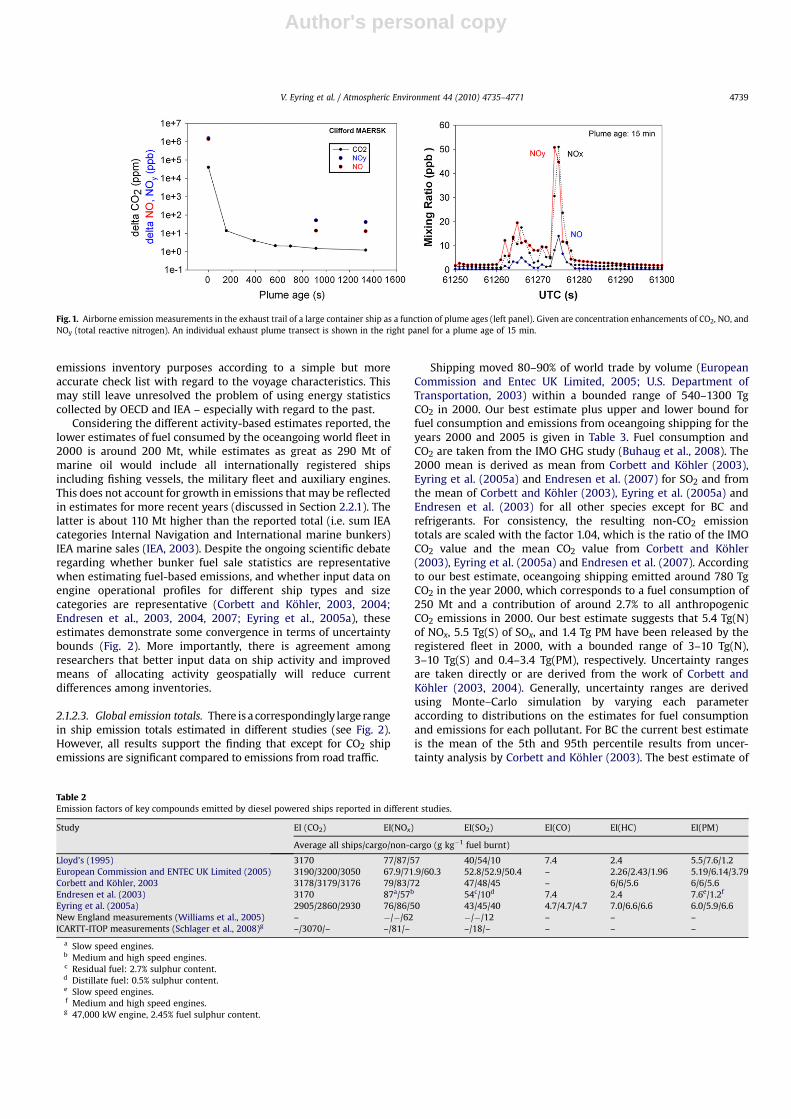
The world fleet is powered mainly by diesel engines, and theemission profiles depend on engine type (slow, medium and highspeed) more than on fuel type for some exhaust compounds (e.g.NOx). The emissions factors for oceangoing vessels are derived froma variety of engine exhaust measurement studies and confirmed byseveral field plume measurements. At the stack, all measurements ofemissions factors used in recent analyses in the U.S., Canada, andEurope are very similar (EPA, 2000; Skjølsvik et al., 2000; EMEP/CORINAIR, 2002; Cooper, 2002; European Commission and ENTEC UKLimited, 2002; Corbett and Kohler, 2003; Eyring et al., 2005a; ICFConsulting, 2005; California Air Resources Board, 2006; LeveltonConsultants Ltd., 2006). Due to limited testing of ship-stacks andvariability in fuel and combustion properties among engine types,some pollutant emissions factors, e.g. PM, are more uncertain ona fleet-average basis. Little is known on the actual split of PM, e.g. intoBC, POM, sulphate, ash, and other particulate matter, and currentemission estimates are based on a few measurements only (Petzoldet al., 2007; Sinha et al., 2003). Emission factors for NOx, SO2, andparticulates were also derived from aircraft measurements in exhaustplumes of known source ships (Williams et al., 2005; Petzold et al.,2007; Schlager et al., 2008), see Fig.1 as an example. Emission indices(emitted mass per kg fuel burnt) were calculated using
EIðXÞ ¼ EIðCO2ÞMX=MCO2D½X�=D½CO2� (1)
where EI(CO2) denotes the CO2 emission index, MX and MCO2the
mole masses of species X and CO2 (44), respectively. D[X] andD[CO2] are the observed enhancements of the mixing ratios in theplumes relative to ambient background concentrations. The CO2
emission index is known with high accuracy (3070 � 20 g CO2/kgfuel) from the carbon mass fraction in ship fuel (85.1%), see, e.g.UNFCCC (2004), and the fraction of carbon that is converted to CO2
for cruise conditions (98.5%). The emission factors for NOx deter-mined from the measurements were in good agreement with thevalues calculated with the emission models for the correspondingengine type and operation conditions (Table 2). Only the SO2
emission factors were lower than expected from the fuel sulphurcontent indicating SO2 loss from the gas phase in the young exhaustplumes. Fridell et al. (2006) compared emission of NOx and CO2 forcargo transported with a small ship and with a large ship, both withcomparable parameters typical for ship transports in Europe. They
found that transport of a unit cargo with a small ship emits moreCO2 by factor 1.8 and slightly more NOx by factor 1.2.
Units for emissions factors are translated from power-based(g k�1 Wh) to fuel-based (kg ton�1 fuel) using specific fuel oilconsumption factors (g fuel k�1 Wh). Both units are reported in theliterature, with fuel-based factors used where fuel records are thebasis for estimates or where atmospheric field studies have derivedemission indices from plume observations.
2.1.2.2. Fuel consumption. Several studies have modelled globalemissions from oceangoing civil ships by combining estimates formarine fuel sales with their respective fuel-based emissions factors(top-down approach, see Section 2.1.1.1). These estimates based onenergy statistics result in a total fuel consumption below 200 Mt in2000 (e.g. Skjølsvik et al., 2000; Olivier et al., 2001; Endresen et al.,2003, 2007; Dentener et al., 2006).
Although emissions estimates and fuel consumption are relatedto the energy used by ships, recent studies call into question thevalidity of relying on the statistics of marine fuel sales. Thesestudies have focused on activity-based estimation of energy andpower demands from fundamental principles (Corbett and Kohler,2003; Eyring et al., 2005a; Wang and Corbett, 2005; ICF Consulting,2005). These approaches estimate fuel consumption for the worldfleet of around 280 Mt year�1 in 2001 and have shown that fuelallocated to international fuel statistics is insufficient to describetotal estimated energy demand of international shipping. Corbettand Kohler (2004) considered alternative input parameters in theiractivity-based fuel consumption and emission model. Theyconclude that alternative assumptions in the input parameterscould reduce their fuel consumption estimate, but not more than14–16%. However, other activity-based studies have reported lowerestimates, considering alternative operation profile. They claim thatthe main reason for the large deviation between activity-based fuelconsumption estimates is the number of days assumed at sea andthat better activity data (per ship type and size categories) ona yearly basis is required when fleet modelling is used to determinethe actual fuel consumption for the entire world fleet (Endresenet al., 2004, 2007).
Recent efforts to apply activity-based methods to regionalinventories have begun to address the inherent undercounting biasin using international marine fuel sales statistics. The Core Inven-tory of Air Emissions in Europe (CORINAIR), under the Co-operativeProgramme for Monitoring and Evaluation of the Long-RangeTransmission of Air Pollutants in Europe (EMEP) funded by theEuropean Environmental Agency (EMEP/CORINAIR, 2002;Woodfield and Rypdal, 2003), adapted better criteria for labellingtraffic as international or domestic that conforms to pollution-inventory guidance requirements rather than IEA energy allocationcriteria (Thomas et al., 2002). Fuel used by ships is allocated for
Table 1Fleet-average summary for 2001 and for ships of 100 GT and more. The table summarizes the number of ships and installed engine power (PMCR) for the main ship classes fromLMIS (2002).
Ship type Allvessels
Cargo vessels Non-cargo vessels Auxiliary engines(gensets)
Militaryvesselsa
All cargoships
Tanker b Containerships
Bulk and combinedcarriers
General cargovessels
Passenger & fishingships, tugboats, others
Number of ships 90,363 43,967 11,156 2759 6457 23,595 45,096 – 1300Number of shipsc (%) 49 12 3 7 27 51PMCR (MW) 343,384 218,733 54,514 46,461 46,297 71,461 67,051 40,000 17,600PMCR
c (%) 77% 19% 16% 16% 25% 23%
a About 300 GT and above (equals approximately 100 t standard displacement and more) including some 520 submarines, 190 of which are nuclear powered. The total navyfleet consist of almost 20,000 military ships (including 750 submarines) with 34,633 main engines and a total installed engine power (MCR) of 172,478 MW.
b Including 1301 crude oil carriers and 1153 gas carriers.c Percent of civilian fleet main engines, excluding auxiliary engines.
V. Eyring et al. / Atmospheric Environment 44 (2010) 4735–47714738
Author's personal copy
emissions inventory purposes according to a simple but moreaccurate check list with regard to the voyage characteristics. Thismay still leave unresolved the problem of using energy statisticscollected by OECD and IEA – especially with regard to the past.
Considering the different activity-based estimates reported, thelower estimates of fuel consumed by the oceangoing world fleet in2000 is around 200 Mt, while estimates as great as 290 Mt ofmarine oil would include all internationally registered shipsincluding fishing vessels, the military fleet and auxiliary engines.This does not account for growth in emissions that may be reflectedin estimates for more recent years (discussed in Section 2.2.1). Thelatter is about 110 Mt higher than the reported total (i.e. sum IEAcategories Internal Navigation and International marine bunkers)IEA marine sales (IEA, 2003). Despite the ongoing scientific debateregarding whether bunker fuel sale statistics are representativewhen estimating fuel-based emissions, and whether input data onengine operational profiles for different ship types and sizecategories are representative (Corbett and Kohler, 2003, 2004;Endresen et al., 2003, 2004, 2007; Eyring et al., 2005a), theseestimates demonstrate some convergence in terms of uncertaintybounds (Fig. 2). More importantly, there is agreement amongresearchers that better input data on ship activity and improvedmeans of allocating activity geospatially will reduce currentdifferences among inventories.
2.1.2.3. Global emission totals. There is a correspondingly large rangein ship emission totals estimated in different studies (see Fig. 2).However, all results support the finding that except for CO2 shipemissions are significant compared to emissions from road traffic.
Shipping moved 80–90% of world trade by volume (EuropeanCommission and Entec UK Limited, 2005; U.S. Department ofTransportation, 2003) within a bounded range of 540–1300 TgCO2 in 2000. Our best estimate plus upper and lower bound forfuel consumption and emissions from oceangoing shipping for theyears 2000 and 2005 is given in Table 3. Fuel consumption andCO2 are taken from the IMO GHG study (Buhaug et al., 2008). The2000 mean is derived as mean from Corbett and Kohler (2003),Eyring et al. (2005a) and Endresen et al. (2007) for SO2 and fromthe mean of Corbett and Kohler (2003), Eyring et al. (2005a) andEndresen et al. (2003) for all other species except for BC andrefrigerants. For consistency, the resulting non-CO2 emissiontotals are scaled with the factor 1.04, which is the ratio of the IMOCO2 value and the mean CO2 value from Corbett and Kohler(2003), Eyring et al. (2005a) and Endresen et al. (2007). Accordingto our best estimate, oceangoing shipping emitted around 780 TgCO2 in the year 2000, which corresponds to a fuel consumption of250 Mt and a contribution of around 2.7% to all anthropogenicCO2 emissions in 2000. Our best estimate suggests that 5.4 Tg(N)of NOx, 5.5 Tg(S) of SOx, and 1.4 Tg PM have been released by theregistered fleet in 2000, with a bounded range of 3–10 Tg(N),3–10 Tg(S) and 0.4–3.4 Tg(PM), respectively. Uncertainty rangesare taken directly or are derived from the work of Corbett andKohler (2003, 2004). Generally, uncertainty ranges are derivedusing Monte–Carlo simulation by varying each parameteraccording to distributions on the estimates for fuel consumptionand emissions for each pollutant. For BC the current best estimateis the mean of the 5th and 95th percentile results from uncer-tainty analysis by Corbett and Kohler (2003). The best estimate of
Fig. 1. Airborne emission measurements in the exhaust trail of a large container ship as a function of plume ages (left panel). Given are concentration enhancements of CO2, NO, andNOy (total reactive nitrogen). An individual exhaust plume transect is shown in the right panel for a plume age of 15 min.
Table 2Emission factors of key compounds emitted by diesel powered ships reported in different studies.
Study EI (CO2) EI(NOx) EI(SO2) EI(CO) EI(HC) EI(PM)
Average all ships/cargo/non-cargo (g kg�1 fuel burnt)
Lloyd’s (1995) 3170 77/87/57 40/54/10 7.4 2.4 5.5/7.6/1.2European Commission and ENTEC UK Limited (2005) 3190/3200/3050 67.9/71.9/60.3 52.8/52.9/50.4 – 2.26/2.43/1.96 5.19/6.14/3.79Corbett and Kohler, 2003 3178/3179/3176 79/83/72 47/48/45 – 6/6/5.6 6/6/5.6Endresen et al. (2003) 3170 87a/57b 54c/10d 7.4 2.4 7.6e/1.2f
Eyring et al. (2005a) 2905/2860/2930 76/86/50 43/45/40 4.7/4.7/4.7 7.0/6.6/6.6 6.0/5.9/6.6New England measurements (Williams et al., 2005) – �/�/62 �/�/12 – – –ICARTT-ITOP measurements (Schlager et al., 2008)g –/3070/– –/81/– –/18/– – – –
a Slow speed engines.b Medium and high speed engines.c Residual fuel: 2.7% sulphur content.d Distillate fuel: 0.5% sulphur content.e Slow speed engines.f Medium and high speed engines.g 47,000 kW engine, 2.45% fuel sulphur content.
V. Eyring et al. / Atmospheric Environment 44 (2010) 4735–4771 4739

Author's personal copy
0.13 Tg BC emitted by oceangoing shipping in 2000 agrees wellwith results from Lack et al. (2008). Emissions of N2O from shipsare very small (0.03 Tg in 2000; Buhaug et al., 2008).
While ship cargoes are not as recognized as a source of globalemissions as ship propulsion, they are important sources of VOCs(methane and non-methane). Initially ship methane emissionswere estimated to be quite low, together with rail at 0.09 Tg
representing only 10% of light-duty vehicles (Piccot et al., 1996).VOCs emissions inventories were later produced using activity-based inventories designed for cargo activities (Endresen et al.,2003), speciating methane from engines to be about 11% andmethane from cargoes to be about 15% of total hydrocarbons,respectively. Eyring et al. (2005a) characterized the methanefraction to be about 13% of total engine hydrocarbon emissions.
100
1.000
10.000
Regist
ered F
leet F
uel U
se
Regist
ered F
leet C
O2
Tg
p
er Y
ear
0.001
0.010
0.100
1.000
10.000
Tg
p
er Y
ear
Traditional Air Pollutants, Black Carbon and HFCs
Corbett and Fischbeck, 1999
Current best estimate
Endresen et al, 2003 Corbett and Koehler, 2003
Endresen et al, 2007 Eyring et al, 2005
Fig. 2. Summary of estimated ranges in global fuel consumption and emissions from maritime shipping for the year 2000. The current best estimate is derived as mean from Corbettand Kohler (2003), Eyring et al. (2005a) and Endresen et al. (2007) for fuel consumption, CO2, and SO2 or Endresen et al. (2003) for all other species except for BC and refrigerants.For BC the current best estimate is the mean of the 5th and 95th percentile results from uncertainty analysis and the source for refrigerants is Devotta et al. (2006). The Corbett andKohler (2003) and Eyring et al. (2005a) results are for 2001 and have been scaled to 2000 fuel consumption and emissions by using the ratio of the total seaborne trade in 2000 and2001 from Fearnleys (2007). Box-plots represent the 5th and 95th percentile results and whiskers extend to lower and upper bounds from explicit uncertainty analysis for fuelconsumption, CO2, NOx, SOx, and PM and from expert judgement for the rest. Uncertainty ranges are taken directly or are derived from the work of Corbett and Kohler (2003, 2004),with extensions for HFCs and cargo methane. Generally, uncertainty ranges are derived using Monte–Carlo simulation by varying each parameter according to distributions on theestimates for fuel consumption and emissions for each pollutant. Note: Emissions do not represent comparative climate impacts. *Registered fleet includes passenger vessels, fishingvessels plus cargo ships, but not military vessels. **Registered fleet engine HC does not include cargo evaporative HC. ***Total NMVOC (NMHC) includes tanker loading (see Table 3of Eyring et al., 2005a).
Table 3Best estimate plus upper and lower bound for fuel consumption and emissions from oceangoing shipping for the years 2000 and 2005.
Year Unit 2000 meana 2000 lower boundb 2000 upper boundb 2005 meanc 2005 lower boundc 2005 upper boundc
Registered fleet fuel used [Mt] 250 120 370 300 150 450Registered fleet CO2 [Tg(CO2)/a] 780 560 1360 960 450 1660Registered fleet NOx [Tg(N)/a] 5.4 3.0 10.4 6.6 3.7 12.7Registered fleet SOx [Tg(S)/a] 5.5 3.2 9.8 6.7 3.9 12.0Registered fleet PM [Tg PM/a] 1.4 0.4 3.4 1.8 0.5 4.1Registered fleet CO [Tg PM/a] 1.18 1.06 1.35 1.44 1.30 1.66NMVOCe,f [Tg NMVOC/a] 1.14 0.37 1.78 1.32 0.46 2.18CH4
e,f [Tg CH4/a] 0.14 0.05 0.23 0.17 0.06 0.28BC [Tg BC/a] 0.13 0.05 0.28 0.16 0.06 0.34POM [Tg POM/a] 0.14 0.12 0.82 0.17 0.15 1.00Refrigerants [Tg/a] 0.003 0.001 0.016 0.004 0.002 0.020
a Fuel consumption and CO2 are taken from the IMO GHG study (Buhaug et al., 2008). The 2000 mean is derived as mean from Corbett and Kohler (2003), Eyring et al.(2005a) and Endresen et al. (2007) for SO2 and from the mean of Corbett and Kohler (2003), Eyring et al. (2005a) and Endresen et al. (2003) for all other species except for BCand refrigerants. For consistency, the resulting non-CO2 emission totals are scaled with the factor 1.04, which is the ratio of the IMO CO2 value and the mean CO2 value fromCorbett and Kohler (2003), Eyring et al. (2005a) and Endresen et al. (2007). The Corbett and Kohler (2003) and Eyring et al. (2005a) results are for 2001 and have been scaled to2000 fuel consumption and emissions by using the ratio of the total seaborne trade in 2000 and 2001 from Fearnleys (2007).
b Lower and upper bounds are derived from explicit uncertainty analysis for fuel consumption, CO2, NOx, SOx, and PM and from expert judgement for the rest. Uncertaintyranges are taken directly or are derived from the work of Corbett and Kohler (2003, 2004), with extensions for HFCs and cargo methane. Generally, uncertainty ranges arederived using Monte–Carlo simulation by varying each parameter according to distributions on the estimates for fuel consumption and emissions for each pollutant.
c To calculate 2005 emissions, the 2000 emissions have been scaled with the ratio of the total seaborne trade (TST) in 2005 (29094) and TST in 2000 (23693) from Fearnleys(2007), see Fig. 4.
d Registered fleet includes passenger vessels, fishing vessels plus cargo ships, but not military vessels.e Not including HC emissions from crude oil transport.f NMVOC from crude oil transport (evaporation during loading, transport, and unloading) in 2000 is 1665 Tg and CH4 is 0.294 Tg from Endresen et al. (2003).
V. Eyring et al. / Atmospheric Environment 44 (2010) 4735–47714740

Author's personal copy
According to the IPCC (Devotta et al., 2006), a small fraction,about 1100 of 35,000 commercial vessels, carry refrigeratedcargoes. HCFC-22 is the common refrigerant in these systems.Nearly all other commercial ships also use HCFC-22 to refrigeratetheir crew food supplies, and operate air conditioning systems.Ammonia refrigerants are also used in shipping. Devotta et al.(2006) estimate ship refrigerant emissions to be less than3000 tons annually. Emissions of CFCs from the world shippingfleet were estimated at 3000–6000 tons for the year 1990 –equivalent to around 1–3% of annual global emissions. Halonemissions from shipping for the same year were estimated to be300–400 tons, or around 10% of world total. More recent figures arenot readily available. It is anticipated that these would showa significant reduction in CFC and halon emissions on account of thephase out of these substances as a consequence of the MontrealProtocol on Substances that Deplete the Ozone Layer and subse-quent amendments (Reynolds and Endresen, 2002).
Fig. 2 presents summary estimates and bounding ranges ofpollutant emissions discussed above, including NOx (as elementalnitrogen), SOx (as elemental sulphur), and particulate matter(PM10), hydrocarbons and methane (from both engines andcargoes), BC and POM (constituents of PM with climate implica-tions), and refrigerants. The figure shows estimated ranges of fueluse and CO2 alongside the other emissions using a log-scale. Themost important insight from Fig. 2 is that nearly all previous esti-mates fall within bounded ranges, and that point estimates usingactivity-based methods are consistently higher than estimatesbased on fuel sales statistics. A second insight is that some emis-sions are much more uncertain than others (e.g. PM, CH4, POM,HFCs). A third important point for policy decisions is that for mostpollutants, the action level for policy decisions may fall below therange of current ‘‘disagreement’’ among point estimates. Forexample, action to create SOx Emission Control Areas under IMOAnnex VI was justified using estimates based on fuel sales, whichfalls near the lower bound for SOx estimates. Moreover, these pointestimates are based on in-year estimates, and must be adjusted forgrowth to compare using a more recent or common year (discussedin Section 2.2.1). Lastly, recent estimates using activity-basedmethods are converging on a narrower range than represented bythese bounded box-whisker plot.
2.1.2.4. Spatial proxies of global ship traffic. Scientific research alsoimproved the geographical distributions of ship emissions so theymore accurately represent world fleet traffic (Corbett and Kohler,2003; Endresen et al., 2003; Dalsøren et al., 2007; Wang et al., 2007).
The spatial distribution of emissions used in EnvironmentalDatabase for Global Atmospheric Research (EDGAR; Olivier et al.,1999; Dentener et al., 2006) was derived from the world’s mainshipping routes and their traffic intensity (Times Books, 1992; IMO,1992; Fig. 3 upper panel) and was one of the first top-downshipping inventories. However, EDGAR is now considered to beunrealistic and more comprehensive inventories represent morerealistic shipping patterns. Corbett et al. (1999) produced one of thefirst global spatial representations of ship emissions using a ship-ping traffic intensity proxy derived from the ComprehensiveOcean-Atmosphere Data Set (COADS), a data set of voluntarilyreported ocean and atmosphere observations with ship locationswhich is freely available. Endresen et al. (2003) improved the globalspatial representation of ship emissions by using ship size (grosstonnage) weighted reporting frequencies from the AutomatedMutual-Assistance Vessel Rescue system (AMVER) data set (Fig. 3middle panel). AMVER, sponsored by the United Coast States Guard(USCG), holds detailed voyage information based on daily reportsfor different ship types. Participation in AMVER was, until veryrecently, limited to merchant ships over 1000 GT on a voyage for 24
or more hours and data are strictly confidential. The participation inAMVER is 12,550 ships but only around 7100 ships have actuallyreported. Endresen et al. (2003) observed that COADS and AMVERlead to highly different regional distributions. Wang et al. (2007)addressed the potential statistical and geographical sampling biasof the International Comprehensive Ocean-Atmosphere Data Set(ICOADS, current version of COADS; Fig. 3 lower panel) and AMVERdatasets, the two most appropriate global ship traffic intensityproxies, and demonstrate (using ICOADS) a method to improveglobal proxy representativeness by trimming over-reportingvessels that mitigates sampling bias, augment the sample data set,and account for ship heterogeneity. Apparent underreporting toICOADS and AMVER by ships near coastlines, perhaps engaged incoastwise (short sea) shipping especially in Europe, indicates thatbottom-up regional inventories may be more representative locally.The three different shipping traffic intensity proxies discussedabove are shown in Fig. 3.
All recent studies report that the majority of the ship emissionsoccur in the Northern Hemisphere within a fairly well defined systemof international sea routes (Skjølsvik et al., 2000; Endresen et al.,2003; Corbett and Kohler, 2003; Wang et al., 2007). The best estimateis that 80% of the traffic is in the Northern Hemisphere, and distrib-uted with 32% in the Atlantic, 29% in the Pacific, 14% in the IndianOcean and 5% in the Mediterranean. The remaining 20% of the trafficin the Southern Hemisphere is approximately equally distributedbetween the Atlantic, the Pacific, and the Indian Ocean. Across allregions, some 70% of ship emissions occur within 400 km of coast-lines, conforming to major trade routes (Corbett et al., 1999). It isimportant to recognize that the significant growth in ship activity inAsian waters over recent years will change the above distribution.
Ship activity patterns depicted by ICOADS, AMVER and theircombination demonstrate different spatial and statistical samplingbiases. None can be judged to represent global ship traffic andemissions better than any other by cross-comparison alone. Thesedifferences could significantly affect the accuracy of ship emissionsinventories and atmospheric modelling, and can be used togetherto perform uncertainty analyses of ship air emissions impacts ona global scale. Researchers have improved the global proxy repre-sentativeness by adjusting the data to mitigate sampling bias,augment sample data set, and account for ship heterogeneity(Endresen et al., 2003; Wang et al., 2007). Even with theseimprovements, global proxy data has limitations. National inven-tories covering coastal shipping may have to be added to theseglobal data – especially where short sea shipping is substantial, asoutlined by Dalsøren et al. (2007). Endresen et al. (2007) alsopointed out that this is important, as ships less than 100 GT typi-cally in coastal operations are not included in the geographicaldistribution (e.g. today some 1.3 million fishing vessels).
Effective monitoring and reliable emission modelling on anindividual ship basis is expected to improve if data from the long-range identification and tracking (LRIT) technology and the auto-matic identification system (AIS) are used. LRIT is a satellite-basedsystem with planned global cover of maritime traffic from 2008. AIStransponders automatically broadcast information, such as theirposition, speed, and navigational status, at regular intervals. Since2004, all ships greater than 300 GT on international voyages arerequired by the IMO to transmit data on their position using AIS. TheLRIT information ships will be required to transmit the ship’s iden-tity, location and date and time of the position. One of the moreimportant distinctions between LRITand AIS, apart from the obviousone of range, is that, whereas AIS is a broadcast system, data derivedthrough LRIT will be available only to the recipients who are entitledto receive such information and safeguards concerning the confi-dentiality of those data have been built into the regulatory provi-sions. Because no interface is planned for LRIT and AIS data, these
V. Eyring et al. / Atmospheric Environment 44 (2010) 4735–4771 4741

Author's personal copy
sources will independently describe common ship activities thatshould help improve the global proxy data and enable betterdevelopment of global networks like STEEM (Wang et al., 2008).
2.2. Shipping growth trends and historical development
This section presents trend indicators corresponding to globaltrade volumes, and discusses some of the specific details charac-terizing historical fleet characteristics.
2.2.1. Growth rates since 2001Over the last 30 years a clear and well understood correspon-
dence is observed between fuel consumption and seaborne trade inton-miles, because the work done in global trade is proportional tothe energy required. The IMO greenhouse gas study chose a lineartrend extrapolation of 3% year�1 for trade to represent the energyand CO2 emissions trend (Skjølsvik et al., 2000). More recentstudies have revealed that the growth in trade over recent decadesis non-linear and that it is higher than 3% year�1 (e.g. Corbett et al.,
Fig. 3. Ship Emissions Allocation Factors (SEAF) from EDGAR (Dentener et al., 2006), AMVER (Endresen et al., 2003), and ICOADS (Wang et al., 2007). SEAF in each grid cell is definedas the fraction of ship emissions in that grid cell of the global total (expressed in millionth of the global total).
V. Eyring et al. / Atmospheric Environment 44 (2010) 4735–47714742

Author's personal copy
2007a). Similarly, Endresen et al. (2007) illustrated strong corre-lation between the world fleet fuel consumption and total seabornetrade in ton-miles (r ¼ 0.97). Recent annual growth rates in totalseaborne trade in ton-miles have been 5.2% on average from 2002to 2007, a lot higher than in past decades (Fearnleys, 2007, see alsoFig. 4). Accordingly, the fuel consumption from 2001 to 2006 hasincreased significantly as the total installed power increased byabout 25% (Lloyd’s Register Fairplay, 2006). Fig. 5 shows the fuelconsumption from 1950 to 2007 as reported in the literature inaddition to the back- and forecast calculated from the time evolu-tion of freight ton-miles.
It is reported that estimated container trade, measured in cargotons, to have grown in 2006 by 11.2%, reaching 1.13 billion tons by2006. Over the last two decades, global container trade (in tons) isestimated to have increased at an average annual rate of 9.8%, whilethe share of containerized cargo in the world’s total dry cargo isestimated to have increased from 7.4% in 1985 to 24% in 2006. Inthis context, it is important to note that over 70% of the value ofworld international seaborne trade is being moved in containers.Chinese ports (including Taiwan Province of China and Hong Kong,China) accounted for 102.1 million TEUs2 in 2005, representingsome 26.6% of the world container port throughput. In 2006preliminary figures show that throughput has increased to 118.6million TEUs, a rise of 16% in 2005 (UNCTAD, 2007). Clearly, theincrease in recent years in shipping particular in Asian waters (seealso Fig. 5) needs to be taken into account in future studies.
2.2.2. Historical fuel consumption and emissionsOver the last 100 years the fleet expanded by 72,000 motor
ships to a total of 88,000, with a corresponding increase in tonnagefrom 22.4 to 553 GT (Lloyd’s Register of Shipping, statistical tables,1964 (year 1900), and world fleet statistics and statistical tables,2000). This growth has been driven by increased demand forpassenger and cargo transport, with 300 Mt cargo transported in1920 (Stopford, 1997) and 5400 Mt in 2000 (Fearnleys, 2003). In1950 the civilian fleet consisted of 30,844 vessels of 100 GT andabove with a total of 84.6 million GT (ISL, 1994; Lloyd’s, 2002).Starting around 1960, the world merchant fleet increased rapidlyand the ship number more than doubled in the period between1960 and 1980. Part of this ship boom was the tanker business,which reached its peak around 1973–1975, and the introduction ofa new type of cargo ship, the container vessel. In general, littleinformation on the historical development of fuel consumption isavailable, with little data published pre-1950 and large deviationsreported for estimates covering the last three decades (see Fig. 5).
Eyring et al. (2005a) produced one of the first estimates for fuelusage over a historical period from 1950 to 2001. They havereported simplified activity-based inventories from 1950 up to1995 using ship number statistics and average engine statistics,while the estimate for 2001 is based on detailed fleet modelling(see Section 2.1.2.2). The results suggest that fuel consumption fromoceangoing ships has increased by a factor of 4.3 from 1950(64.5 Mt) to 2001 (280 Mt). Uncertainties in this estimate arise fromthe fact that reliable input data such as detailed shipping andengine as well as engine performance statistics, activity data andthe detailed fleet structures before 1976 are not available. Endresenet al. (2007) reported more detailed activity estimates from 1970 to2000 per year. They suggested that activity-based estimates forpast fuel consumption and emissions must take into account vari-ation in the demand for sea transport and operational and technicalchanges over the years, to better represent the real fuel
consumption and corresponding emissions. Their results suggestthat the fleet growth is not necessarily followed by increased fuelconsumption, as technical and operational characteristics havechanged. They also reported annual fuel consumption before theFirst World War, and detailed fuel-based estimates (based on sales)from 1925 up to 2000 (Fig. 5). The results indicated that oceangoingships had a yearly fuel consumption of about 80 Mt of coal (cor-responding to 56.5 Mt heavy fuel oil) before the First World War.This increased to a sale of about 200 Mt of marine fuel oils in 2000(including the fishing fleet), i.e. about a 3.5-fold increase in fuelconsumption. Ships emitted around 229 Tg (CO2) in 1925 (Endresenet al., 2007) and grew to 638–800 Tg (CO2) in 2000/2001 (Endresenet al., 2007; Corbett and Kohler, 2003; Eyring et al., 2005a). Thecorresponding SO2 emissions are about 2.5 Tg (SO2) in 1925 andbetween 8.7 and 12.03 Tg (SO2) in 2001. The CO2 emissions per tontransported by sea have been significantly reduced as a result oflarger and more energy efficient ships. For comparison, the tonnageincreased from 22.4 million GT in 1900 to 84.6 million GT in 1950,and 553 million GT in 2000.
2.3. Future scenarios compliant with currentinternational legislation
Merchant ships in international traffic are subject to IMOregulations and emissions from ships in international trade areregulated by ANNEX VI of MARPOL 73/78. Here we discuss onlythose future scenarios that are compliant with present-day IMOregulations. These scenarios are subsequently used in this study toassess the impacts on atmospheric chemistry, climate and humanhealth. National or regional regulations call for even more stringentNOx and SOx limits than those given by IMO (e.g. EPA, 2002). Asa result, compliance with emission regulations through techno-logical improvements will impact ship operators and the tech-nology in use, and will thus impact on the emissions. Those otherfuture scenarios that consider possible emission reductions andimprovements of fuel efficiency are presented in Section 6.
Ship activity has increased steadily over the last two decadesand is predicted to continue growing for the foreseeable future.Most studies on future scenarios take historic trends for somerecent period and extrapolate with adjustment for expected changein trends, e.g. the response to economic and population driversaffecting global trade or consumption.
The TREMOVE maritime model (Ceuster et al., 2006; Zeebroecket al., 2006) estimates fuel consumption and emissions trendsderived from forecast changes in ship voyage distances (maritimemovements in km) and the number of port calls. It includes everyyear from the base year 1995 until 2020. According to the TREMOVE
,0
5,000
10,000
15,000
20,000
25,000
30,000
35,000
1987
1989
1991
1993
1995
1997
1999
2001
2003
2005
TS
T [b
illio
n to
nn
e-m
iles]
-3
0
3
6
9
12
15
18
21
An
nu
al G
ro
wth
in
T
ST
[%
]
2007 es
t.
Fig. 4. World seaborne trade (TST) in billion ton-miles and corresponding annualgrowth rate from 1987 to 2007. Source: Fearnleys (2007).
2 TEU (20-foot equivalent unit). An equivalent unit is a measure of containerizedcargo capacity equal to one standard 20 ft (length) � 8 ft (width) container.
V. Eyring et al. / Atmospheric Environment 44 (2010) 4735–4771 4743

Author's personal copy
report, maritime fleet and vehicle kilometres grow annually by 2.5%for freight and 3.9% for passengers, while port callings grew by 8%compared to the previously used input figures. Other estimates thatare published outside of the journal literature also confirm thegeneral importance and sometimes suggest higher growth rates(e.g. Meszler Engineering Services analysis, ICCT, 2007).
The IMO study on greenhouse gas emissions from ships(Skjølsvik et al., 2000) used fleet growth rates based on two marketforecast principles, validated by historical seaborne trade patterns:(1) world economic growth will continue; and (2) demand forshipping services will follow the general economic growth. TheIMO study correctly described that growth in demand for shippingservices was driven by both increased cargo (tonnage) andincreased cargo movements (ton-miles), and considered that thesecombined factors make extrapolation from historic data difficult.Nonetheless, their forecast for future seaborne trade (combinedcargoes in terms of tonnage) was between 1.5 and 3% annually. TheIMO study applied these rates of growth in trade to representgrowth in energy requirements. The ENTEC study (EuropeanCommission and ENTEC UK Limited, 2002) adopted growth ratesfrom the IMO study.
However, a constant annual growth of the world’s real grossdomestic product (GDP) does not necessarily mean the sameincrease in seaborne trade. During the past two decades real GDPaccording to the statistics of the International Monetary Fund (IMF,2004) grew by 2.8% p.a. on average, whereas international tradeexperienced an average annual growth rate of 6.2% (IMF, 2004).Since 1985 the world seaborne trade gained 3.3% in terms ofvolumes and 3.6% p.a. in terms of ton-miles on average (Fearnleys,2004; Clarkson, 2004). The lower growth rate of seaborne tradecompared to international trade results from the fact that inter-national trade is measured in monetary values while seabornetrade is measured in weight. Based on the historical correlationbetween the total seaborne trade and GDP over the time period1985–2001, Eyring et al. (2005b) estimated future world seabornetrade in terms of volume in million tons for a specific ship trafficscenario in a future year, using a linear fit to historical GDP data.
This represents one of the only studies to forecast growth inseaborne trade for energy and emissions purposes at rates fasterthan GDP. Following the annual growth rate in GDP of the four IPCCSRES storylines (2.3–3.6%), seaborne trade in the four future shiptraffic demand scenarios increased by 2.6–4.0% p.a. According tothis study, fuel consumption by the oceangoing fleet could increasefrom 280 Mt in 2001 to 409 Mt by 2020 and 725 Mt by 2050. Thesescenario calculations demonstrate that significant technologicalimprovements are needed to offset increased emissions due togrowth in seaborne trade and cargo energy intensity. Withoutstringent emission reduction strategies, CO2 and SO2 emissionsfrom ships would more than double present-day values by 2050and NOx emissions could exceed the values from present-day globalroad transport (Fig. 6, technology scenario 4).
It is important to note that the future in the scenario calculationsfrom Eyring et al. (2005b) starts in 2002 and thus does not includethe recent unexpected high growth rates between 2002 and 2007(see Section 2.2.1). Further work is currently underway withrespect to the latest growth rates and with respect to the likelyupdated technology pathways.
3. Impact on atmospheric composition
The majority of emissions from shipping are injected into theatmosphere in the form of coherent plumes, often in relativelypristine parts of the atmosphere. To assess the impact of shippingon the atmospheric composition with the help of global models theemission totals are distributed over the globe with spatial proxiesof global ship traffic derived in various ways (see Sections 2.1.2.3and 2.1.2.4) and are instantaneously spread onto large inventorygrid boxes, usually 1� longitude � 1� degree latitude, withoutaccounting for dispersion, transformation and loss processes on thesubgrid scale. Ship emissions occur locally at relatively highconcentrations in relation to the atmospheric backgroundconcentrations. The emissions are diluted by mixing with theambient air. During the dilution process the emitted species arechemically transformed, secondary species (e.g. ozone) are formed
0,0
50,0
100,0
150,0
200,0
250,0
300,0
350,0
400,0
450,0
1950 1960 1970 1980 1990 2000 2010
Fu
el C
on
su
mp
tio
n (M
t)
Eyring et al., JGR, 2005
Freight-Trend Intertanko, August 2007
Freight-Trend Corbett and Köhler, JGR, 2003
Freight-Trend Eyring et al., JGR, 2005
Endresen et al., JGR, 2007
Freight-Trend Endresen et al., JGR, 2007
Int'l Marine Bunker Sales (IEA 2006)
Point Estimates from the Studies
Fig. 5. World fleet fuel consumption (civilian, military, and auxiliary) and international marine bunker fuel statistics in Mt from different estimates. The symbols indicate theoriginal estimates for individual years and the solid lines show the original trend estimates from these studies. The dashed lines show the back- and forecast calculated from thetime evolution of freight ton-miles with the point estimates from 2001 (Corbett and Kohler, 2003; Eyring et al., 2005a), 2000 (Endresen et al., 2007), 2007 (Gunner, 2007), and 1997(IEA, 2006) taken as the reference year.
V. Eyring et al. / Atmospheric Environment 44 (2010) 4735–47714744

Author's personal copy
and they are already partially removed from the atmosphere by wetand dry deposition. These processes non-linearly depend on theconcentrations of the primary emissions, the atmospheric back-ground concentrations and on the actual meteorological state of theatmosphere such as height and stability of the marine boundarylayer, vertical wind profile or the presence of clouds. Otherimportant factors involve the insolation depending on latitude andtime of the day. The chemistry and transport in the marineboundary layer (MBL) is discussed in Section 3.1, while near–fieldprocesses and impacts of shipping on the large-scale are assessed inSections 3.2 and 3.3, respectively.
3.1. Chemistry and transport in the marine boundary layer
3.1.1. Chemistry in the marine boundary layerTo a large extent the chemistry of the MBL, as with the rest of the
troposphere, is determined by the oxidation of primary emittedspecies and their subsequent reactions (Seinfeld and Pandis, 1998).
The main reaction pathways of relevance for the climate activecompounds (e.g. CH4, O3 and sulphate particles) are the NOx-cata-lysed formation of ozone, the gaseous and aqueous oxidation of SO2
to sulphate aerosol, and the destruction of methane by OH. Thehalogen-catalysed destruction of ozone can also be significant inthe MBL.
The main oxidising agent in the troposphere is the OH radical.This is produced through the ultra-violet photolysis of ozone (R1;see Table 4) followed by reaction of the O(1D) radical with watervapour (R2) and through conversion of the HO2 radical to OH bynitric oxide (NO) (R7). Thus NOx emissions from shipping increasethe OH radical through two routes, directly by reaction with HO2,and indirectly by generating ozone (see below). This extra OHremoves methane and other hydrocarbons from the atmosphere.
The formation of ozone is initiated by the reaction of OH withspecies such as CO and CH4 forming hydroperoxyl radical (HO2) andmethyl peroxy radical (CH3O2), respectively (R3–R6). OH reactionswith more complex hydrocarbons are analogous to CH4, generating
Fig. 6. Possible range of future NOx emissions in Tg(NO2), CO2 in Tg(CO2), SOx in Tg(SO2), CO in Tg(CO), HC in Tg(HC), and PM in Tg(PM) according to four different technologyscenarios (TS1–4) and four different ship traffic demand scenarios (DS1–4). Results for the technology scenario 1 (TS1) are shown for different ship traffic demand scenarios (DS1–4)with solid lines in black, those for TS2 with long dashed lines, for TS3 with short dashed lines, and for TS4 with dotted lines (from Eyring et al., 2005b, their Fig. 4; Copyright, 2005;American Geophysical Union; Reproduced by permission of American Geophysical Union).
V. Eyring et al. / Atmospheric Environment 44 (2010) 4735–4771 4745

Author's personal copy
the related organic peroxy radicals. Net ozone formation in the MBLis then a result of competition between ozone formation and sinkreaction cycles. In the presence of NOx, reaction of peroxy radicalswith NO leads to formation of NO2 which photolyses to give ozone(R7–R10). However, at low concentrations of NOx, peroxy radicalsprimarily react through peroxy–peroxy self- and cross reactionsyielding hydrogen and organic peroxides (R11 and R12). Ozone ismainly destroyed by photolysis (R1 and R2), reaction with HO2
(R13) and deposition to the ocean surface. Ozone chemistry in theMBL is thus very sensitive to changes in concentrations of NOx.Fleming et al. (2006) performed calculations of ozone formation inthe MBL during the NAMBLEX experiment and found a lineardependency of ozone production rate on NO concentration. Emis-sions far away from land in relatively clean environment areparticularly important from the point of view of the formation oftropospheric ozone. The efficiency of ozone production from NOx
emissions is much greater in cleaner environments (Liu et al., 1987;Lin et al., 1988). There are few NOx sources over the oceans otherthan ships. NOx itself has a short lifetime in the atmosphere butcontinental emissions of NOx are often collocated with significantconcentrations of the acetyl peroxy radical (either from anthropo-genic or biogenic sources). The reaction with NOx (R14) formsperoxy acetyl nitrate (PAN) which is longer lived than NOx. PANformed over the continents can be transported to the marineatmosphere where it can decompose to release NOx thus providingan additional NOx source.
The ozone chemistry in the MBL can also be significantlyaffected by reactive halogen species (Dickerson et al., 1999;Carpenter et al., 2003). The sources of these are autocatalytic
halogen activation mechanisms (Vogt et al., 1996) and photolysis ofI-containing organic compounds emitted by macroalgae in coastalregions (O’Dowd et al., 2002). In the halogen activation mechanism,gaseous HOBr and HOCl are scavenged on sea-salt aerosol wherethey form only slightly soluble BrCl and Br2 that are released back tothe gas phase (R16–R18, R20, R22). Halogen atoms formed byphotolysis of the dihalogens or the I-containing organic compoundsreact with ozone to form halogen monoxides. These recycle in thegas phase via reaction sequences involving HOX (X ¼ Br, Cl or I;reactions R17–R19) that catalytically destroy ozone analogously toatomic chlorine and bromine cycling in the stratosphere. Thehalogen activation mechanism also acts as a sink for HO2 (HO2
consumed in R18 is transferred to H2O(aq) by R20 and R22).Formation of halogen nitrates XNO3 in R23 and their heterogeneousreactions on sea-salt and in particular on acidic sulphate particles(R24, R25) can significantly decrease the lifetime of NOx in the MBL.In box model simulations supported by measurements of gas phaseand aerosol composition in the tropical MBL, Pszenny et al. (2004)showed that heterogeneous reactions of halogen nitrates onsulphate particles were responsible for approximately 25% of thetotal sink of NOx in the MBL. Importance of these reactions on sea-salt particles varied with sea-salt concentrations from 5% of thetotal NOx sink at moderate sea-salt concentrations to as much as60% at high sea-salt concentrations. Heterogeneous reactions ofdinitrogen pentoxide (N2O5) (R26, R27) can also influence the NOx
lifetime, however, these reactions were not found to be importantin the MBL.
The MBL is important for production of aerosol particles.Primary aerosol in the form of sea-salt particles is produced frombursting bubbles and by direct release of sea-spray from the wavecrests. Oxidation of dimethyl sulfide (DMS) released by phyto-plankton produces sulphate aerosol that is active as cloudcondensation nuclei (CCN) (Charlson et al., 1987), and methyl sul-phonic acid (MSA) aerosol that does not act as CCN (R35–R39). MostDMS oxidation is initialized by the OH radical (R35 and R36), witha contribution from the nitrate radical (NO3) at night (R37). Ship-ping will therefore increase the DMS oxidation rate, particularly inwinter. This means that more DMS is oxidised over the ocean,which may increase CCNs.
SO2 emissions from shipping are oxidized to sulphate primarilyin the aqueous phase (in cloud droplets and sea-salt particles) byhydrogen peroxide (H2O2) and ozone (R29–R34) and also in the gasphase by the OH radical (R28). The largest impact of shipping onsulphate chemistry is through the direct emissions of SO2.However, increases in the OH radical due to NOx emissions willenhance the gaseous oxidation pathway. This pathway is importantsince it leads to new particle generation which is important for theclimate forcing whereas aqueous oxidation adds mass to existingparticles.
Dry deposition to the ocean surface occurs for many of thereactive species discussed here (O3, NO2, SO2, sulphate). This isgenerally at a lower rate than to the continental surface, and thedeposition velocity is typically 1 mms�1 for ozone. Even so, depo-sition to the ocean is still an appreciable loss rate for ozone since thephotochemical loss is slower in the cleaner environment. Collinset al. (2009) showed that around a third of the ozone generated byshipping was lost to deposition, the majority of which was over theocean. It might be expected that dry deposition is more rapid inrougher seas. Fairall et al. (2007) calculated an enhancement inozone deposition of up to a factor of 3 due to ocean turbulence. Thisis not generally taken into account in modelling studies.
3.1.2. Transport in the marine boundary layerA major part of ship emissions (excluding emissions in ports and
in the vicinity of coastlines) are emitted in or transported to the
Table 4Important chemical reactions in the marine boundary layer.
[R1] O3 þ hn (l < 290 nm)/O2 þ O(1D)[R2] O(1D) þ H2O/2 OH[R3] OH þ CO/H þ CO2
[R4] H þ O2/HO2
[R5] OH þ CH4/H2O þ CH3
[R6] CH3 þ O2/CH3O2
[R7] HO2 þ NO/OH þ NO2
[R8] CH3O2 þ NO/CH3O þ NO2
[R9] NO2 þ hn/O(3P) þ NO[R10] O(3P) þ O2 þ M/O3 þ M[R11] RO2 þ HO2/ROOH þ O2
[R12] HO2 þ HO2/H2O2 þ O2
[R13] HO2 þ O3/OH þ 2 O2
[R14] NO2 þ CH3COO25PAN[R15] NO2 þ OH þ M/HNO3 þ M[R16] X2 þ hn/2X (X ¼ Cl or Br)[R17] X þ O3/XO þ O2
[R18] XO þ HO2/HOX þ O2
[R19] HOX þ hn/OH þ X[R20] HOX5HOX(aq)[R21] HX5X� þ Hþ
[R22] HOX(aq) þ X� þ Hþ5X2 þ H2O[R23] NO2 þ XO/XNO3
[R24] XNO3 þ H2O(aq)/HOX(aq) þ HNO3(aq)[R25] XNO3 þ X�(aq)/X2(aq) þ HNO3(aq)[R26] N2O5 þ H2O(aq)/HNO3(aq) þ HNO3(aq)[R27] N2O5 þ X�(aq)/XNO2 þ HNO3(aq)[R28] SO2 þ OH þ H2O/H2SO4
[R29] SO25SO2(aq)[R30] SO2(aq)5HSO3
�(aq) þ Hþ(aq)[R31] HSO3
�(aq)5SO32�(aq) þ Hþ(aq)
[R32] HSO3�(aq) þ H2O2(aq)/SO4
2�(aq) þ Hþ(aq)[R33] HSO3
�(aq) þ O3(aq)/SO42�(aq) þ Hþ(aq) þ O2
[R34] SO32�(aq) þ O3(aq)/SO4
2�(aq) þ O2
[R35] DMS þ OH/CH3S(OH)CH3
[R36] DMS þ OH þ O2/CH3SO2 þ HCHO þ H2O[R37] DMS þ NO3 þ O2/CH3SO2 þ HCHO þ HNO3
[R38] CH3S(OH)CH3/MSA or SO2
[R39] CH3SO2/MSA or SO2
V. Eyring et al. / Atmospheric Environment 44 (2010) 4735–47714746
Author's personal copy
MBL. As mixing and transport in the MBL has specificities thatsubstantially differ from conditions that determine mixing andtransport of the land-based emissions, and since these conditionsimpact on the effect of these emissions on chemistry, this sectiondiscusses micrometeorological properties of the MBL.
The large heat capacity of water and efficient mixing processesin the upper oceanic mixed layer makes the distinguished propertyof the MBL the remarkable spatial and temporal homogeneity intemperature. The air–sea temperature differences tend to be small,except close to the coasts. If the air temperature is much lower thanthe sea surface temperature (SST), vigorous convection will reducethe temperature difference, and, except for areas with large hori-zontal gradients in SST, horizontal advection can not maintain theimbalance. Hence the surface layer is nearly neutral over almost allof the oceans (Pasquill stability class D) (Arya, 1988). When warmair moves over cooler water, the ‘very stable’ condition corre-sponding Pasquill stability class F occurs and movement of cold airover warmer water leads to ‘unstable’ condition correspondingPasquill stability class B (Song et al., 2003).
Due to the small air–sea temperature difference the majorcomponent of the energy balance at the sea surface is the latentheat of evaporation, which is typically 50–200 W m�2, an order ofmagnitude larger than the sensible heat flux, typically 0–30 W m�2.Only during episodes of cold air outbreaks over warmer seas thesensible heat becomes an important part of the energy balance(Arya, 1988).
The transfer of momentum from the atmosphere to the oceanpartly generates surface waves and partly drifts currents andturbulences in the upper layers of the ocean. Relation betweenthese two modes is complex and not easy to determine. Near thewater surface (few wave heights) a downwelling–upwellingpattern of wave motion generates both positive and negativevertical momentum flux (Sullivan et al., 2004). The wind profilemeasurements above few wave heights show validity of theMonin–Obukhov relation
U=u� ¼ ð1=kÞ � lnðz=z0 �Jmðz=LÞÞ; (2)
where u* is the friction velocity, k the von Karman’s constant takenas 0.4, z0 the roughness length and jm(z/L) the stability function formomentum that describes deviation from the neutral wind profileand depends on stability index z/L where z is the height above thesurface and L is the Monin–Obukhov length (Edson and Fairall,1998). The roughness length z0 of the sea surface has a rangebetween around 10�4 and 10�3 m (Arya, 1988) and depends on thewind and wave fields. The simplest and widely used relationbetween z0 and u* is described by Charnock’s formula based ondimensional arguments (Charnock, 1955) z0 ¼ a � (u*2/g), wherea is an empirical Charnock’s constant, also called dimensionlessroughness, and g is the gravitational acceleration. The value ofa derived from block-averaged datasets from many differentobservation sites at open sea is 0.01–0.02 (Charnock, 1955: 0.012,Garratt, 1977: 0.0144, Wu, 1980: 0.0185). The underlying wave field(the wave age) also affects the Charnock’s constant (Johnsson et al.,1998) and it varies largely when the water surface is affected by thecoast (Arya, 1988).
Most often the MBL is perceived as being well mixed between thesurface layer and the capping inversion (this layer is also called‘mixed layer’). When cumulus clouds are forming near the top of thislayer, where the latent heat from condensation allows the newlyformed clouds to penetrate the capping inversion and transport fluidto the overlaying layer, the concept of MBL has sometimes beenextended to this overlaying layer (Cotton et al., 1995).
The MBL is frequently covered with clouds. It is cloud free inareas where warm air is transported over colder air and a stable
and shear-driven BL is formed. The tropical MBL is associatedwith deep convection and formation of cumulus clouds. Themixed layer height zmbl extends from a few hundred meters up toover 1000 m and the overlaying layer extends typically up to2 km in Pacific and Atlantic ocean and up to 4.5 km in Indianocean (Ramana et al., 2004 and references there in). Variation ofthickness of the MBL results in exchange between the MBL andthe free troposphere. Russell et al. (1998) determined the bi-directional entrainment rates during the ACE-1 experiment. Thethickness of the MBL zmbl at mid latitudes extends typicallybetween 500 and 1000 m. During the daytime the subcloud layerof the MBL can be decoupled from the overlaying stratocumuluslayer due to the shortwave radiation heating of the cloud. In theafternoon the mixing throughout the whole MBL will reoccur.This process occurs especially in the MBL topped with a thickcloud layer and is of importance for the air–sea exchange anddispersion of pollutants in the MBL.
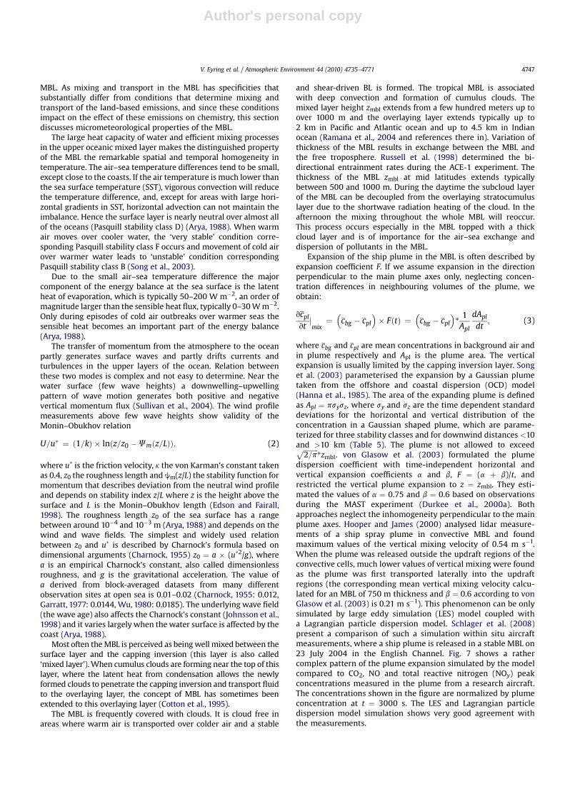
Expansion of the ship plume in the MBL is often described byexpansion coefficient F. If we assume expansion in the directionperpendicular to the main plume axes only, neglecting concen-tration differences in neighbouring volumes of the plume, weobtain:
vcpl
vtjmix¼�
cbg � cpl
�� FðtÞ ¼
�cbg � cpl
�*
1Apl
dApl
dt; (3)
where cbg and cpl are mean concentrations in background air andin plume respectively and Apl is the plume area. The verticalexpansion is usually limited by the capping inversion layer. Songet al. (2003) parameterised the expansion by a Gaussian plumetaken from the offshore and coastal dispersion (OCD) model(Hanna et al., 1985). The area of the expanding plume is definedas Apl ¼ psysz, where sy and sz are the time dependent standarddeviations for the horizontal and vertical distribution of theconcentration in a Gaussian shaped plume, which are parame-terized for three stability classes and for downwind distances <10and >10 km (Table 5). The plume is not allowed to exceedffiffiffiffiffiffiffiffiffi
2=pp
*zmbl. von Glasow et al. (2003) formulated the plumedispersion coefficient with time-independent horizontal andvertical expansion coefficients a and b, F ¼ (a þ b)/t, andrestricted the vertical plume expansion to z ¼ zmbl. They esti-mated the values of a ¼ 0.75 and b ¼ 0.6 based on observationsduring the MAST experiment (Durkee et al., 2000a). Bothapproaches neglect the inhomogeneity perpendicular to the mainplume axes. Hooper and James (2000) analysed lidar measure-ments of a ship spray plume in convective MBL and foundmaximum values of the vertical mixing velocity of 0.54 m s�1.When the plume was released outside the updraft regions of theconvective cells, much lower values of vertical mixing were foundas the plume was first transported laterally into the updraftregions (the corresponding mean vertical mixing velocity calcu-lated for an MBL of 750 m thickness and b ¼ 0.6 according to vonGlasow et al. (2003) is 0.21 m s�1). This phenomenon can be onlysimulated by large eddy simulation (LES) model coupled witha Lagrangian particle dispersion model. Schlager et al. (2008)present a comparison of such a simulation within situ aircraftmeasurements, where a ship plume is released in a stable MBL on23 July 2004 in the English Channel. Fig. 7 shows a rathercomplex pattern of the plume expansion simulated by the modelcompared to CO2, NO and total reactive nitrogen (NOy) peakconcentrations measured in the plume from a research aircraft.The concentrations shown in the figure are normalized by plumeconcentration at t ¼ 3000 s. The LES and Lagrangian particledispersion model simulation shows very good agreement withthe measurements.
V. Eyring et al. / Atmospheric Environment 44 (2010) 4735–4771 4747

Author's personal copy
3.2. Near-field processes
It is recognised now that subgrid-scale processes should beaccounted for in global models with a resolution of several hundredkilometres because of non-linearities in atmospheric processes. Inplume processes that need to be considered include oxidation ofNOx, scavenging of HNO3, ozone formation, oxidation and hetero-geneous removal of SO2, impact of ship-emitted and backgroundparticles on plume chemistry and processing of particles affectingtheir physical properties.
3.2.1. Nitrogen compounds and ozoneDavis et al. (2001) proposed that in the plume the reaction of NO
with HO2 (R7) leads to enhanced OH mixing ratios and thus to anenhanced rate of the main sink reaction for NOx (R15). Fast oxida-tion of NOx in concentrated plumes due to elevated OH levels couldlead to a substantial decrease in lifetime of NOx compared to thebackground. Additional chemical loss of NOx can be through PANformation, through nighttime formation of NO3 and N2O5, followedby their heterogeneous oxidation on aerosol, and through NO2
oxidation by halogen oxides (R23) yielding halogen nitrates. Inhighly concentrated parts of the plume and in cases when theplume is emitted to a NOx pre-polluted background with alreadyenhanced OH levels, reaction R15, being also a sink for OH, cancause OH depletion in the plume, which leads on contrary toincreased NOx lifetime in the plume.
Chen et al. (2005) inferred from measurements in a ship plumea chemical NOx lifetime of about 2 h, almost four times shorter thancalculated for background air. Ship plume modelling studies ofSong et al. (2003) and von Glasow et al. (2003) showed NOx life-times of a factor of 2.5–10 and 4, respectively, shorter in the shipplume than in the background. Photo-stationary calculations witha box model in Chen et al. (2005) showed that 80% of the loss wasdue to R15 and a remainder due to PAN formation. Song et al.(2003) found that elevated levels of NO3 and N2O5 shortened theNOx lifetime during the nights. The observed NOx loss rates in theship plume measured by Chen et al. (2005) were 30% larger thanthose estimated with the model. Measured HNO3 levels in theplume were only about 20% of the mixing ratios estimated by themodel simulations indicating a rapid HNO3 loss in the plume notincluded in the model, possibly uptake of HNO3 on particles. NOy/CO2 measurements in a ship plume aged 0.5 h by Schlager et al.(2008) also indicate a loss of 50% gas phase NOy. A modelling studyby Franke et al. (2008) found an increased NOx lifetime compared toNOx lifetime in the background during the first hours of thesimulation, which was only slightly reduced later on. The NOx
emission source strength in the Franke et al. (2008) study wasmuch higher than in previous studies (a large container shipemitting 145 g NOx/s, compared to an average ship emitting 47 gNOx/s) leading to much higher NOx mixing ratios at the initial stageof the plume. Also model simulations of the ship plume measuredby Schlager et al. (2008) showed increased lifetime of NOx during
1–2 h after the emission. A sensitivity study has shown that at highNOx background concentrations, when the ozone formation is inperoxy radical limited regime, the increased lifetime would persistover the entire lifetime of the plume. The chemical lifetimes of NOx
in the ship plumes from different studies are summarised inTable 6.
Neglecting the plume processes in global models may lead to anoverestimation of O3 formation. In early stages of the plume themain reason of this overestimate is that the plume becomes limitedin peroxy radicals that would react with NO in the ozone-formingNOx cycle (R7–R10). Later, in more diluted stages of the plume thedecreased NOx mixing ratios in plume caused by its reduced life-time have further effect on ozone formation. von Glasow et al.(2003) quantified the effect of neglecting the plume processes ina grid of a global model by comparing a box model includingmultiple plumes with a box model including continuous homoge-neous emissions of a same magnitude. They found 50% lower O3
mixing ratios when the plume dispersion was considered. Frankeet al. (2008) compared box model simulations of a single plumeentraining background air using the Gaussian plume modelparameterization (PD case) with a box model where the same shipemissions were instantaneously dispersed into a large grid box (IDcase). The ozone formation in the PD case was found to be 70%lower than in the ID case.
3.2.2. Sulphur compoundsIn contrast to NOx, Davis et al. (2001) and Eyring et al. (2007)
found significant underestimation of the SO2 mixing ratios in theMBL simulated by the global models compared to observations.Model simulations in Davis et al. (2001) produced significantincrease of SO2 mixing ratios in MBL from ship emissions. Theensemble mean increase of SO2 from shipping in Eyring et al.(2007) was small, so the authors questioned whether the under-estimation of SO2 in the marine boundary layer in the models isdue to the ship emission inventory or due to the underestimationof another source (e.g. DMS), overestimation of a sink (e.g.oxidation), errors associated with simulating specific events (e.g.horizontal/vertical transport and mixing), or a combination ofseveral factors, opened. Davis et al. (2001) put forward a hypoth-esis that in contrary to oxidation of NOx, where its increasedconcentration in ship plumes and ship lanes leads to shortening ofNOx lifetime through increased OH concentrations, the SO2
oxidation by OH is only a minor oxidation pathway and the pHsensitive oxidation by heterogeneous reactions, the dominantoxidation pathway for SO2, may be significantly inhibited by H2SO4
produced in oxidation. This theory was, however not confirmedwith measurements in plumes. On contrary, the SO2 concentra-tions measured in aged ship plumes were significantly lower thanvalues expected from the sulphur fuel content and the dilution asgiven by the plume excess CO2 in all studies (Chen et al., 2005;Williams et al., 2005; Schlager et al., 2008). The reason for thisdiscrepancy is still to be investigated.
Table 5Formulas for lateral and vertical dispersion coefficients, sy and sz for downwind distances� as a function of time t after the plume release for moving shipsa (reformulated fort ¼ x/ur from Song et al., 2003).
Over-water stability class sy, mb sz, m
B (unstable) x < 10 km 0.08tu(1 þ 0.0001tu)�1/2 0.06tux > 10 km 0.08tu(1 þ u/ur)
�1/2 0.06tuD (neutral) x < 10 km 0.04tu(1 þ 0.0001tu)�1/2 0.03tu(1 þ 0.0015tu)�1/2
x > 10 km 0.04tu(1 þ u/ur)�1/2 0.03tu(1 þ 0.0015tu)�1/2
F (stable) x < 10 km 0.02tu(1 þ 0.0001tu)�1/2 0.008tu(1 þ 0.0003tu)�1
x > 10 km 0.02tu(1 þ u/ur)�1/2 0.008tu(1 þ 0.0003tu)�1
a Here, the wind speed is u and ur defines the magnitude of the resultant vector of the wind speed and ship speed.b The minimum value of the leading constant in the sy formulas is 0.5/u, where u is the wind speed.
V. Eyring et al. / Atmospheric Environment 44 (2010) 4735–47714748

Author's personal copy
3.2.3. Particlesvon Glasow et al. (2003) studied the effect of processes on
heterogeneous particles emitted from the ship and on the back-ground sea-salt and sulphate particles in plume. They found thatthe partly soluble particles emitted from the ship (sulphate-coatedparticles) have the potential to substantially decrease the NOx
lifetime and ozone formation in the plume only under extremelyhigh particle emissions due to reactions of NO3, N2O5, BrNO3 andClNO3. Heterogeneous processes on ship-emitted soot were foundto be negligible. Background sea-salt and sulphate aerosol mayhave a larger effect on the plume chemistry than ship-emittedparticles. This effect may well be caused by changes of NOx, O3, andOH mixing ratios in the background air in the two sensitivity runs.
Petzold et al. (2007) measured the transformations of aerosolsin a plume of a large container ship. An extensive change in thesize-distribution was observed from a count median diameter of52 nm of the raw exhaust to 70 nm in the young plume and 100 nmin the plume aged 0.5 h. The strong nucleation mode measured inthe raw exhaust was completely depleted in the aged plume. Themass of BC and the associated number of non-volatile combustionparticles were well correlated with the excess CO2 in the plume.From the decay of the non-volatile particle concentration in theaging plume a maximum plume lifetime of about 24 h was esti-mated by Petzold et al. (2007) for a well mixed MBL.
3.2.4. Effective emissionsSeveral approaches to parameterise the non-linear plume
effects in global models have been suggested. Petry et al. (1998)defined effective emission indices (EEI) for aviation, an approachwhere the emissions are modified in a way that after beingdispersed into a global model grid cell, the effective emissionsapproach at a certain time horizon the same mixing ratios as if theyhad undergone plume dispersion. Esler (2003) introduced a moregeneral concept of equivalent emissions where the modification ofemissions is calculated from the mixing history of the plume andapplied it on a simplified NOx–CO–O3–HOx system. Franke et al.(2008) further developed and applied the EEI concept of Petry et al.(1998) on ship plume emissions, however only for a limited set ofconditions. They presented variation of the EEI of NOx, O3 and H2O2
with time of the day of the emission and with the source strength ofNOx. The EEI are expressed as drelX ¼ dX/DNOx, where dX is theeffective emission of NOx, O3 and H2O2 (in mol or mol s�1) andDNOx is the actual emission of NOx. The EEI of ozone variedbetween �20% for emission at nighttime to�750% for emissions inthe middle of the day. The EEI of NOx were also negative withlargest absolute values at nighttime (�7%) and smallest aroundnoon (�1%). The EEI of H2O2 showed similar pattern of diurnalvariation as EEI of NOx with values of �20% at night and þ5% atnoon. If this concept should be used in a global model, extensive
Fig. 7. (a) Plume concentrations normalised by concentrations at plume age t ¼ 3000 s, (cpl � cbg)/(clp � cbg)t¼3000 plotted against the age of the plume. Maximum normalisedconcentrations in LES and Lagrangian particle dispersion coupled model (dashed line) and (b) measured peak normalised concentrations. The dotted line on both panels is a meanconcentration development in a plume described by normalised concentration C ¼ 3000/t, t in s (Schlager et al., 2008).
Table 6Chemical lifetimes of NOx in observed and model-simulated ship plumes and ratios of the background air to plume lifetimes. The source strength of NOx (emitted as NO), QNO
(in g(NO)/s) is given in column 3. Notes in the last column indicate how the NOx lifetimes were derived: The measured lifetime is inverse value of the first order loss ratecoefficient of measured NOx enhancement due to ship emissions relative to the enhancement of a non-reactive plume tracer as derived in Chen et al. (2005). The modelledlifetime is the photochemical lifetime of NOx defined by first order loss rates LNOx ¼ k1[OH][NO2] þ k2[NO3][DMS] þ k3[NO3] þ 2*k4[N2O5], where k1–k4 are the appropriatereaction rate constants.
Fuel type QNO sNOx in plume sNOx(bg)/sNOx(pl) Note to sNOx
g s�1 h d.l.
Chen et al. (2005) Residual 13.4 1.7/2.4 3.8/2.7 Measured/modelledd.t.t.o. Residual – 1.9/2.25 3.4/2.9 Measured/modelledSchlager et al. (2008) Residual 184 128/6.3 0.15/0.99 Model, early plume/average
d.t.t.o. ship corridorSong et al. (2003) Residual 4 10.5–25.4 1.3–1.8 Model, tropics – mid. lat.d.t.t.o. Residual 20 5.1–14.5 2.4–3.2 Model, tropics – mid. lat.von Glasow et al. (2003) Residual 16.5 2.8/7.5 5.3/3.6 Model, early plume/averageFranke et al. (2008) Residual 145 5/8 0.6/1.01 Model, early plume/average
V. Eyring et al. / Atmospheric Environment 44 (2010) 4735–4771 4749

Author's personal copy
calculations of EEI for combinations of meteorological and chemicalconditions and larger set of different source strengths would benecessary.
3.3. Large-scale effects on atmospheric composition
Global modelling studies (Lawrence and Crutzen, 1999; Capaldoet al., 1999; Kasibhatla et al., 2000; Davis et al., 2001; Endresenet al., 2003; Eyring et al., 2007; Dalsøren et al., 2007; Collins et al.,2009) have generally used similar global totals for NOx and SO2
emissions from ships, about 3 Tg (N) year�1 and 4 Tg (SOx) year�1.The distributions used have been more variable. The EDGAR2.0distribution contains narrow shipping lanes (Fig. 3, upper panel),while the COADS distribution uses data from ship position reportsand is more widespread (similar to ICOADS, Fig. 3, lower panel).Endresen et al. (2003) used AMVER as their preferred distribution(Fig. 3, middle panel) and compared the ozone response to thesimulated response using COADS and PF (Purple Finder). TheCOADS distribution is more concentrated at higher latitudes andover the North Atlantic than AMVER. The PF distribution is similarto AMVER but more concentrated towards the coasts. Lauer et al.(2007) applied the three emission inventories displayed in Fig. 3 ina global aerosol climate model to address uncertainties in emissiontotals and global distributions on the impact of oceangoing ship-ping on aerosols, clouds and the radiation budget.
3.3.1. Large-scale chemistry effects of ozone precursor emissionsBeing a short-lived chemical compound, NOx enhancement from
ship emissions is closely dependent on the routes. NOx increases of200 to more than 1000 ppt in the shipping lanes were simulated byLawrence and Crutzen (1999), and increases of 200–500 pptderived from the multi-model mean of ten state of the art atmo-spheric chemistry models have been reported by Eyring et al.(2007). Both studies used the EDGAR dataset (Fig. 3, upper panel).The other emissions datasets (COADS, AMVER, PF) are morerealistic and more spread out. Using one of the latter emissiondistributions, NOx increases of over 200 ppt were calculated inKasibhatla et al. (2000) over the northern Atlantic and Pacificoceans. Increases of 100–150 ppt over the same regions werecalculated by Dalsøren et al. (2007), Endresen et al. (2003) andDavis et al. (2001). Estimated background concentrations varyconsiderably between models, with the earlier models thatincluded little or no NMVOCs (non-methane VOCs) and PANchemistry (e.g. Lawrence and Crutzen, 1999) having very lowbackground NOx levels, around 10 ppt or less. A model that didinclude higher hydrocarbons (Endresen et al., 2003) simulated Julynorth Atlantic background values of 20–50 ppt in the continentaloutflow, compared to below 5 ppt inside the Azores anticycloniccirculation. In the coastal regions of North America and Europe, NOx
enhancements from shipping can be 200–300 ppt in a higherresolution model (Dalsøren et al., 2007). Using the EDGAR emis-sions database (Eyring et al., 2007; Collins et al., 2009) givesparticular high NOx values in the Baltic due to an overestimate ofemissions from this area in the inventory.
The lifetime of shipping NOx (defined as the burden divided bythe emission rate) can be calculated from Fig. 9 of Eyring et al.(2007). Total troposphere NOx burden increased by about 0.012 Tgfor emissions of 3.1 Tg year�1 (excluding two outlier models),resulting in a lifetime of shipping NOx of around 1.5 days.
Some comparisons of shipping generated NOx in large-scalemodels with observations have shown significant overestimates(Kasibhatla et al., 2000; Davis et al., 2001; Endresen et al., 2003).These studies suggested that subgrid-scale processes not includedin the global models rapidly convert NOx to total reactive nitrogen(NOy) in ship plumes. However these models overestimated the
NOx concentrations even without shipping. The amount of obser-vational data available to compare to is very limited and compari-sons are very sensitive to the choice of the dataset. Eyring et al.(2007) found disagreement between their multi-model averageNO2 simulations and the observations used in Davis et al. (2001),but agreement with a larger observational dataset from Emmonset al. (2000).
Observations from satellite have confirmed the existence of highNO2 concentrations along shipping lanes (Beirle et al., 2004; Richteret al., 2004, see Fig. 8). The implications for the larger scale ofneglecting small-scale plume chemistry depend on the resolutionof the models, and the size of the tracks. From the point of view oflarge-scale composition impacts, there is not enough observationaldata to confirm or refute the various emission datasets used byglobal models. There are sound chemical reasons why spreadingshipping plumes over the size of grid squares used by global modelscould overestimate the NOx, OH and ozone responses (see Sections3.1 and 3.2). Plume model studies have not yet come up witha simple reduction factor for the NOx emissions that could beapplied to global models. Thus in a crude attempt to compensate forplume effects, global models tend to use a lower NOx emission totalof w3 Tg(N) year�1 rather than the estimate of w5 Tg(N) year�1
recommended in Table 3.Modelling studies generally simulate increases in ozone due to
shipping NOx emissions of up to 12 ppb in the central NorthAtlantic, and central North Pacific in July. Ozone enhancementstend to peak in mid-ocean, and not in the coastal regions, due to thehigher NOx levels there from continental sources. Eyring et al.(2007) found much smaller increases over the Pacific due to thesmaller and more concentrated emissions in the EDGAR datasetused. In January, ozone increases of 2–4 ppb are found in thetropical and sub-tropical oceans except in the Eyring et al. (2007)study, which has lower tropical emissions. In winter, Eyring et al.(2007) found shipping NOx leads to ozone destruction in northernEurope. This is strongest over the Baltic and countries bordering itand is due to the removal of HOx through the reaction R15. In thehigh-latitude winter where there is little insolation, HOx levels arealready low so the OH þ hydrocarbon oxidation is the rate deter-mining step for ozone production (R3 and R5). This ozonedestruction is not found in other studies and may be exacerbateddue to the high level of shipping emissions in the Baltic in theEDGAR distribution.
To identify changes in coastal ozone production requires a high(by global modelling standards) resolution model. The Dalsørenet al. (2007) study with a 1.8� � 1.8� resolution identifies regions ofhigh ozone production from shipping in smaller seas with busyshipping, such as the North Sea, Baltic, Mediterranean, Red Sea andPersian Gulf where enhancements exceed 14 ppb (see Fig. 9).
The climate impact of the extra ozone generated by emissions ofNOx from shipping largely depends on the change to the total ozonecolumn. The distribution and magnitude are quite sensitive to theemissions distribution used. In Dalsøren et al. (2007) these changesare generally concentrated in a band from the equator to 45�N (2–3DU) with a local maximum over the Persian Gulf and Arabian Sea(up to 5 DU). The Eyring et al. (2007) simulations do not show thiszonal band. They have a maximum south of India of 1.2 DU,otherwise increased ozone columns of up to 1.0 DU are found overthe North Atlantic. Again, the lack of ozone changes at lower lati-tudes is likely to be due to the EDGAR shipping distribution and willhave a significant effect on the calculated radiative forcing fromshipping (Section 5.2).
None of the studies listed here included any of the halogenchemistry described in Section 3.1.1 in their models. As a result theyare likely to slightly overestimate the marine boundary layer ozoneconcentrations. The impact of CO, VOCs and direct methane from
V. Eyring et al. / Atmospheric Environment 44 (2010) 4735–47714750

Author's personal copy
Fig. 8. NOx signature of shipping in the Indian Ocean. Upper panel: Tropospheric NO2 columns derived from SCIAMACHY data from August 2002 to April 2004. Lower panel:Corresponding distribution of NOx emissions from shipping taken from an emission inventory (from Richter et al., 2004, their Fig. 3; Copyright, 2004; American Geophysical Union;Reproduced by permission of American Geophysical Union).
Fig. 9. Ozone change at the surface due to year 2000 ship emissions simulated by the OsloCTM2 for the months (top left) January, (top right) April, (bottom left) July and (bottomright) October (from Dalsøren et al., 2007, their Fig. 5; Copyright, 2007; American Geophysical Union; Reproduced by permission of American Geophysical Union).
V. Eyring et al. / Atmospheric Environment 44 (2010) 4735–4771 4751

Author's personal copy
shipping on ozone is very small, generally less than 0.1 ppb(Endresen et al., 2003; Eyring et al., 2007).
3.3.2. Methane lifetimeEmissions of NOx increase the concentrations of the OH radical
and hence reduce the methane lifetime. Reductions in methanelifetime due to shipping NOx vary between 1.5% (Dalsøren et al.,2007; Eyring et al., 2007) to 0.4 years (w5%) (Lawrence and Crut-zen, 1999; Endresen et al., 2003). The reaction between methaneand the OH radical is very temperature dependent. Hence methaneis oxidised principally in the tropics in the lower troposphere. Thusit might be expected that the models using the EDGAR distribution,which has little NOx enhancement in the tropics, would show theleast effect on methane lifetime. However, there seems littleobvious relationship between the methane impact in the modelresults published so far and the emission distribution used. It islikely that other aspects of the model formulations are moreimportant. Four of the five models reporting methane lifetimes inEyring et al. (2007) calculated decreases of 0.13 years (1.56%) withthe fifth model calculating nearly twice this amount.
Hoor et al. (2008) show that compared to other forms oftransport, shipping has the greatest effect on the methane lifetime.This is because the NOx emissions are released into a cleaner,environment and have larger contributions in the tropics thanland-based transport. Aircrafts have a smaller effect as their emis-sions are away from the lower troposphere where most methaneoxidation occurs.
The decrease in methane lifetime and consequent decrease inthe methane concentrations leads to a longer term decline in theozone concentrations that may offset some or all of the direct ozoneproduction from the NOx emissions. Derwent et al. (2008) foundthat the ozone response to the methane decrease due to land-basedNOx emissions from Asia cancelled out about half of the directozone production as a global average. The ozone decrease is muchmore globally homogenous than the increase thus it is importantfor climate forcing (Section 5.2) but less important for air quality.
3.3.3. Large-scale chemistry effects of aerosol emissionsand their precursors
Ship emissions are responsible for up to 60% of the July surfaceSO2 concentrations over large areas of the North Atlantic and NorthPacific, and for more than 30% of the concentrations of the rest ofthe Northern Hemisphere oceans (Capaldo et al., 1999). Thechemistry-transport model (CTM) results also revealed that ship-ping contributes up to 5–20% of the non-sea-salt sulphateconcentrations in coastal regions over land, demonstrating theimportance of including ship emissions in regional air qualitystudies. These findings are confirmed in an independent study byLauer et al. (2007). Generally oceanic SO2 observations are under-estimated by models (Davis et al., 2001; Eyring et al., 2007) evenwhen shipping emissions are included. Thus shipping SO2 emis-sions may be underestimated if anything. As SO2 is primarilycontrolled by aqueous processes, unlike NOx it is expected that SO2
is largely independent of enhanced OH in the plume (Davis et al.,2001).
Ship emissions contribute 10–40% to sulphate concentrationsover most of the Northern Hemisphere oceans (Lauer et al., 2007).The fractional increases depend on the assumed background. Overthe remote oceans sulphate comes mainly from DMS and isa function of the DMS emission rates and chemistry in the models(R35–R39). Shipping at 2000 levels contributes about 3% to theglobal sulphate loading (Endresen et al., 2007; Eyring et al., 2007).Sulphur emissions might reduce air quality over land, e.g. bycontributing to sulphate aerosol concentration or sulphate depo-sition. Globally shipping contributes 5% of the total sulphur
deposition, and around 3% to the deposition over land (Collins et al.,2009). Ships contribute 5–10% of the sulphate deposition overcoasts of Europe, North America and China (Endresen et al., 2003;Collins et al., 2009; Dalsøren et al., 2007). The precise numbers varywith distance from the coasts. These calculations have beenundertaken with global models that are not able to resolve coastalareas well enough to give more than approximate estimates.Contributions of shipping to aerosol components other thansulphate are small. Lauer et al. (2007) calculate contributions to BCof 0.4–1.4%, to POM of 0.1–1.1%, and to nitrate aerosol of 0.1–2.3%.The large ranges in these estimates reflect the very large uncer-tainty due to the three different emission inventories used.
4. Impacts on air quality, ecosystems and human health
About 70% of the emissions from oceangoing shipping occurwithin 400 km of the coastlines along the main trade routes (Cor-bett et al., 1999). Thereby, ship emissions can have an impact on theair quality in coastal regions and may partly offset the decline ofland-based sources and coastal pollution due to national controlmeasures (Schlager and Pacyna, 2004). The addition of NOx and SO2
from ships also contributes to acidification of the ocean (Doneyet al., 2007). On the global scale these effects are small, but could bemore significant in shallower coastal waters where shipping isconcentrated.
4.1. Regional impact on atmospheric composition
Regional impacts of ship emissions include enhancements ofNOx, CO, VOCs, and SO2 boundary layer gas concentrations andsubsequent perturbations of ozone and other photochemicalproducts, increase of the concentration of particulates (sulphateaerosol, POM, BC), and enhanced deposition of acidifying andeutrophying sulphur and nitrogen compounds. In addition, there isa significant local impact on pollution in the vicinity of majorharbours (Canepa and Georgieva, 2005).
Model studies of the regional impact of ship emissions havebeen performed for the Atlantic Ocean seaboard of Europe (Jonsonet al., 2000; Derwent et al., 2005; Collins et al., 2009) the PacificBasin (Davis et al., 2001), the United Kingdom (Dore et al., 2006),the Scandinavian countries (Dalsøren et al., 2007), and the Medi-terranean region (Marmer and Langmann, 2005). Note that thesemodels are of varying resolution. Derwent et al. (2005), Collins et al.(2009), Davis et al. (2001), and Dalsøren et al. (2007) used globalmodels with resolutions of w500, w250, 265, and w200 kmrespectively. Jonson et al. (2000), Dore et al. (2006) and Marmerand Langmann (2005) used regional models with resolutions of 50 ,5 and w50 km. The resolution of the models affects their ability tosimulate coastal regions, although the finest resolution model usesstatistical meteorology with winds from wind roses and depositionaccording to constant drizzle, which may affect its ability tosimulate the transport of pollutants near coast. For Europe, themodelled contribution of shipping to summertime mean surfaceozone concentrations from emissions of NOx and VOC precursorsvary from 2 to 4 ppb (5–15%) over the coasts of north-westernEurope (Derwent et al., 2005; Collins et al., 2009). Additionalregional ozone impacts are simulated for the Mediterranean regionand the Baltic Sea.
The conditions in the Mediterranean region during summer(slow transport and mixing, high solar radiation intensity, limitedwash out) favour in particular the accumulation of primary shipemissions and production of secondary emissions (Marmer andLangmann, 2005). According to model simulations, secondarysulphate aerosols from shipping account for 54% of the mean
V. Eyring et al. / Atmospheric Environment 44 (2010) 4735–47714752

Author's personal copy
sulphate aerosol concentration in this region during the summerseason (Fig. 10).
Coastal areas of north-western Europe and north-western NorthAmerica are substantially impacted by nitrate and sulphate depo-sition from shipping. In Europe the modelled maximum annualsulphate deposition from ship emissions of 400 mg S m2 year�1
occurs over the North Sea and Baltic Sea (Derwent et al., 2005). Thisis about 50% of the total sulphur deposition in these regions. Alongthe western coasts of the UK and Scandinavia, the calculatedpercentage of total sulphur deposition from shipping rangebetween 10 and 25% (Dore et al., 2006; Dalsøren et al., 2007; Collinset al. 2009).
There are only a few measurement studies on the regionalimpact of ship emissions. Satellite measurements from the GOMEand SCIAMACHY instrument clearly detected enhanced NO2
tropospheric vertical column densities along international shippingroutes in the Indian Ocean (Beirle et al., 2004; Richter et al., 2004;see Fig. 8). Aircraft survey flights across the ship corridors off thecoast of Brittany revealed very inhomogeneous concentration fieldsof shipping-related trace species (Schlager et al., 2008). A multitudeof ship plumes were detected in the vicinity of the main shippingroutes, aged between minutes and up to 5 h (Fig. 11). The measuredship plumes of different ages were often superimposed on eachother and showed concentration enhancements in NO, NOy, SO2, COand CO2. Also ship engine combustion aerosol particles weredetected in the aged plumes (Petzold et al., 2007). Along theshipping lanes, the measured ozone concentrations were up to5 ppb lower compared to values observed outside the corridors asexpected from the reaction of fresh NO ship emissions with ozoneto NO2. These observations are in accordance with results froma regional model for the experimental conditions.
There is also a considerable local impact of shipping-relatedemissions on air quality in the vicinity of major harbours, inparticular, from NOx, SO2, PM, and VOCs emissions. Ship manoeu-vring in harbours contributes about 6% of NOx and 10% of SO2 tototal shipping emissions (Corbett and Fischbeck, 1997). Besidesmanoeuvring, loading and unloading of tankers also contributesubstantially to harbour emissions since this is a highly energyconsuming process (Wismann and Oxbol, 2005). The harbouremissions often occur near major residential areas and can betransported far inland due to local land–sea breeze winds. Forexample, near the waterways of the port of Rotterdam shippingcauses an enhancement of the surface NO2 mixing ratio of 5–7 ppb(Keuken et al., 2005).
4.2. Impact on ecosystems and human health
Local and regional air quality problems in coastal areas andharbours with heavy traffic are of concern because of their impacton human health. Furthermore, emissions from ships are trans-ported in the atmosphere over several hundreds of kilometres, andthus can contribute to air quality problems on land, even if they areemitted over the sea. This pathway is especially relevant for ozoneand the deposition of sulphur and nitrogen compounds, whichcause acidification of natural ecosystems and freshwater bodiesand threaten biodiversity through excessive nitrogen input (Cofalaet al., 2007).
Due to the non-linear nature of ozone chemistry, the effects ofshipping depend on the magnitude of the emission change, and onthe choice of scenario for the land-based emissions. Ozone is toxicto plants (Ashmore, 2005), affecting growth (e.g. crop yield) andappearance. The potential for sulphate and nitrate deposition tocause ecosystem change can be defined by the critical loads. Theeffects on sulphate aerosol levels and deposition fluxes of sulphateaerosols and oxidised nitrogen species are larger, and are signifi-cant compared to expected changes in land-based emissions. Onaverage shipping increases current sulphate aerosol, and sulphateand nitrate deposition over Europe by about 15% (Collins et al.,2009). Sulphate deposition increases the acidity of soils, rivers andlakes. This harms ecosystem growth. Nitrate deposition increasesthe available nitrogen of soils (eutrophication; Stevens et al., 2004;Galloway et al., 2003; Cofala et al., 2007). This can harm ecosystemsthrough asymmetric growth in nitrogen poor regions (e.g. algae inrivers and lakes, and lichens and mosses in hillsides), in someregions encouraging invasive alien species.
Shipping impacts on human health through the formation ofground-level ozone and particulate matter. Cofala et al. (2007)provided an assessment of the health and environmental impactsof shipping scenarios in Europe for the year 2020. They find thatcompared to land-based sources, at least some of the maritimeemissions have less health and environmental impacts since theyare released sometimes far from populated areas or sensitiveecosystems. However, they also find that in harbour cities shipemissions are in many cases a dominant source of urban pollutionand need to be addressed when compliance with EU air qualitylimit values for, e.g. fine particulate matter is an issue. An increasein ship emissions will counteract the envisaged benefits of thecostly efforts to control the remaining emissions from land-basedsources in Europe. Technologies exist to reduce emissions from
Fig. 10. Calculated seasonal mean (June/July/Aug.) of sulphate concentration (mg S m�3) at lowest model level over Europe from land-based emissions (left panel) and shipemissions (right panel). From Marmer and Langmann, 2005, their Fig. 6. Copyright 2005 Elsevier.
V. Eyring et al. / Atmospheric Environment 44 (2010) 4735–4771 4753

Author's personal copy
shipping beyond what is currently legally required. Epidemiolog-ical studies also consistently link ambient concentrations ofparticulate matter to negative health impacts, including asthma,heart attacks, hospital admissions, and premature mortality.Mortality resulting from PM emission from ships has been esti-mated by either estimating loss of life expectancy in months (Cofalaet al., 2007) or by using total number of premature deaths (Corbettet al., 2007b). Previous assessments of regional shipping-relatedhealth impacts focused on European or Western US regions, butignored long-range and hemispheric pollutant transport (CaliforniaAir Resources Board, 2006; Cofala et al., 2007). This undercountsoceangoing shipping impacts within local and regional jurisdic-tions. Recent results by Corbett et al. (2007b) indicate that ship-ping-related PM emissions are responsible for around 60,000cardiopulmonary and lung cancer deaths annually, with mostdeaths occurring near coastlines in Europe, East Asia, and SouthAsia. This number is bounded by a range of 20,000–104,000premature deaths when considering the uncertainties due toemission inventories and models used in this study. Based onprevious estimates of global PM2.5-related mortalities (Cohen et al.,2005), the Corbett et al. (2007b) estimates indicate that 3–8% ofthese mortalities are attributable to marine shipping. Cohen et al.
(2005) estimate that approximately 712,000 cardiopulmonarydeaths are attributable to urban outdoor PM2.5 pollution annually.Thus, the relationship between concentrations and mortalityappears nearly proportional within reasonable percentage uncer-tainty bounds. Uncertainties of the results are detailed in theSupporting Information of Corbett et al. (2007b).
5. Radiative forcing and impact on climate
In addition to the impact on atmospheric composition andhuman health, ship emissions have an impact on climate throughchanges in clouds (Section 5.1) and RF (Section 5.2). RF is a commonmetric to quantify climate impacts from different sources in units ofW m�2, since there is an approximately linear relationship betweenglobal mean radiative forcing and change in global mean surfacetemperature (Forster et al., 2007). Other climate metrics are dis-cussed in Section 5.3.
5.1. Impact on clouds
The perturbation of a cloud layer by ship-generated aerosolpotentially changes the cloud reflectivity. This can be identified byelongated structures in satellite images known as ship tracks(Section 5.1.1). In addition to ship tracks, aerosol emissions fromshipping can also affect clouds on a larger scale after dispersion.The impact of shipping on aerosol properties and on large-scaleclouds is assessed in Section 5.1.2.
5.1.1. Ship tracksOf all anthropogenic sources, ship-stack effluents provide the
clearest demonstration of the indirect aerosol effect on cloudalbedo. Curves of larger reflectance in cloud fields are observed insatellite imagery and identified as ship tracks. The first observationsof ship tracks were presented by Conover (1966) and the manysubsequent observations confirm they are a recurrent phenomenon(e.g. Coakley et al., 1987; Durkee et al., 2000a; Segrin et al., 2007).Such perturbations of the marine stratiform cloud field are char-acterised as long-lived, narrow, curvilinear regions of enhancedcloud reflectivity which occur downwind of ships. An example ofship tracks appearing as bright features in satellite data is given inFig. 12.
The brightness of a cloud observed from space is determinedprimarily by its visible optical thickness s, which for drops largecompared to wavelength can be approximated as
s ¼ 3LWP2rr
(4)
where LWP is the liquid water path, r is density of water and r is theparticle effective radius. Using this approach Twomey et al. (1968)concluded that observed increased optical thickness in ship trackswas consistent with the addition of CCN to a cloud layer with dropconcentrations of about 1–10 drops cm�3, i.e. a clean maritimeboundary layer. This simple description captures the essence ofship track formation and is widely accepted.
Airborne measurements in a cloud free environment abovea cargo ship showed that approximately 12% of exhaust particles actas CCN (Hobbs et al., 2000). Several studies have shown that thedroplet concentration in the ship tracks was enhanced significantlyover the ambient cloud and that the effective radius was reduced(Albrecht, 1989; Radke et al., 1989; Durkee et al., 2000b; Ferek et al.,2000; Schreier et al., 2006). Taylor et al. (2000) summarised theresults of 11 aircraft flights off the west coast of North Americaduring the Monterey Area Ship Track (MAST) experiment. Theimpact of the aerosol emitted from the ships was found to be very
Fig. 11. Mixing ratios of NOy, NO, and SO2 measured during two ship corridor transectsacross the English Channel (Schlager et al., 2008).
V. Eyring et al. / Atmospheric Environment 44 (2010) 4735–47714754

Author's personal copy
dependent on the background cloud microphysics. If the ambient orbackground cloud was of continental influence (and thus containeda higher typical CCN concentration than clean maritime air) thecloud was found to be relatively insensitive to further aerosolemissions, with only a weak microphysics signature in the shiptracks. However, if the background clouds were pristine maritimestratiform then increases in droplet concentration of a factor of 2,and reduction in droplet size of up to 50%, were measured.
A detailed description of the average or composite ship trackcharacteristics for the entire MAST observation period is given inDurkee et al. (2000a). The set of ship tracks examined during theMAST experiment formed in marine boundary layers that werebetween 300 and 750 m deep, and no tracks formed in boundarylayers above 800 m. The tracks form in regions of high relativehumidity, small air–sea temperature differences, and moderatewinds (average of 7.7 � 3.1 ms�1). The composite ship track is296� 233 km long, 7.3� 6 h old, and 9� 5 km wide. The ship is, onthe average, 16 � 8 km from the head of the ship track along therelative wind vector and corresponds to a time of 25 � 15 min. Theexperiment showed a high dependence of ship track developmenton the amount of sulphur in the shipping fuel.
Ship emissions can increase the concentration of CCN to over 10times that of clean air, to about 1000 CCN per cm3 (Durkee et al.,2000c). As the total amount of water in polluted and unpollutedclouds at a particular height is about the same, the water in pollutedclouds is distributed over a much larger number of smaller droplets.The precipitation process is therefore highly sensitive to the size ofthe initial cloud droplets (e.g. Rogers and Yau, 1989). These smallerwater droplets are then less likely to grow into larger drops ofprecipitation size, extending the lifetime of the cloud andincreasing reflectivity. Ackerman et al. (1995) used numericalsimulations to show that ship track lifetimes could be in excess ofa day. Ship track measurements have yielded strong hints, but notclear evidence, that precipitation is affected by exhaust from ships.Albrecht (1989) showed that for ship tracks measured off the coastof California on 13 June 1976, the droplet size-distributions werenarrower and the droplet count was lower, which directly corre-sponded to a notable reduction in drizzle. During an aircraftcampaign off southern California, Radke et al. (1989) observed anincrease in cloud liquid water and a decrease in drizzle-size dropsin ship tracks. Ferek et al. (2000) also noticed a reduction in drizzledrops in ship tracks off Washington but no associated increase in
cloud liquid water. During the MAST experiment Ferek et al. (2000)used aircraft measurements to report that significant changes incloud droplet size-distribution, as well as reductions in drizzle fluxand concentrations of drops larger than 50 mm radius, wereobserved in ship tracks when drizzle was more uniformly presentin the ambient cloud.
A satellite study of clouds forming in the region of the EnglishChannel showed a trend of increasing cloud albedo and decreasingcloud top temperature (Devasthale et al., 2006), which may berelated to the impact of ship emissions. The global distribution ofship tracks from 1 year of AATSR data has been reported by Schreieret al. (2007) and from ATSR/2 data by Campmany et al. (2009).Fig. 13 shows the percent coverage of ship tracks derived fromAATSR measurements in 2004. It shows the predominant area forship track occurrence is a latitude band between 30� and 60� N inboth the North Atlantic and the Pacific Ocean. In the SouthernHemisphere ship tracks are much less frequent and are concen-trated between 10� and 30� S off the west coasts of southern Africaand Australia.
5.1.2. Large-scale impact on cloudsShip plumes mix with the ambient air and are able to affect the
surrounding clouds on a larger scale than visible ship tracks. Toquantify the overall effect, global aerosol model studies or satellitetrend analyses are needed. The model simulations by Lauer et al.(2007) reveal that the effect of changes in particle numberconcentration, aerosol size-distribution and particle compositiondue to ship emissions on clouds is mainly confined to the lowertroposphere, from the surface up to about 1.5 km. This implies thatregions with a frequent high amount of low clouds above theoceans are most susceptible to ship emissions. Such regions coin-cide with dense ship traffic over the Pacific Ocean west of NorthAmerica, and over the Atlantic Ocean west of southern Africa and inthe North eastern Atlantic Ocean. In particular, accumulation modeparticles act as efficient condensation nuclei for cloud formation.
Whereas the cloud liquid water content is only slightlyincreased in these simulations, effective radii of cloud dropletsdecrease, leading to cloud optical thickness increase up to 5–10%depending on geographic region and ship emission inventory used.The sensitivity of the results is estimated by using three differentemission inventories for present-day conditions. According to thesestudies, shipping increases the aerosol number concentration, e.g.up to 40% in the size range of the Aitken mode (typically <0.1 mm)in the near surface layer over the Northern Atlantic.
Above the main shipping routes in the Atlantic Ocean the modalmean diameter of the Aitken mode decreases from 0.05 to 0.04 mm.Due to subsequent growth processes such as condensation of sul-phuric acid vapour onto pre-existing particles or coagulation, someparticles emitted by shipping grow into the next larger size range ofthe accumulation mode (typically >0.1 mm). Accumulation modeparticles can act as additional cloud condensation nuclei. Thechanges in chemical composition (Section 3.3.3), particle numberconcentration, and size-distribution cause an increase in aerosoloptical thickness above the oceans, which is related particularly toenhanced scattering of incoming solar radiation by sulphate,nitrate, ammonium, and associated aerosol liquid water. Increasesin total aerosol optical thickness up to 8–10% are found over theIndian Ocean, the Gulf of Mexico and the North eastern Pacific,depending on the ship emission inventory.
5.2. Radiative forcing
Ship emissions of CO2, SO2, NOx and other O3 precursors perturbatmospheric concentrations of greenhouse gases (CO2, CH4 and O3),and aerosols (mainly sulphate, SO4), causing both positive and
Fig. 12. Ship tracks over the Gulf of Biscay (colour composition from AVHRR on 27January 2003).
V. Eyring et al. / Atmospheric Environment 44 (2010) 4735–4771 4755

Author's personal copy
negative contributions to direct radiative forcing (RF) of climate. Inaddition, ship-derived aerosols cause a significant indirect RF, viachanges in cloud microphysics (see Section 5.1). As CO2 is a wellmixed greenhouse gas, its atmospheric lifetime (>100 year) ismuch longer than global atmospheric mixing timescales, so shipCO2 emissions generate a RF in just the same way as any other CO2
source. SO2 and NOx are reactive species with much shorter life-times (days). Emissions of these species generate SO4 and O3, whichthemselves have lifetimes of days to weeks in the troposphere.Perturbations to SO4 and O3, and hence their RFs, have regional-scale structure, and are closely related to their precursor sourcedistributions. Emissions of NOx, and the O3 they form, lead toenhanced levels of the hydroxyl radical (OH), increasing removalrates of CH4, generating a negative RF (Wild et al., 2001). Because ofthe decadal CH4 lifetime, this RF has a global signature.
Table 7 summarises estimates of the present-day contribution ofship emissions to these different RF components from several
studies (Capaldo et al., 1999; Endresen et al., 2003; Eyring et al.,2007; Lee et al., 2007; Lauer et al., 2007; Dalsøren et al., 2007;Fuglestvedt et al., 2007). These studies used a variety of shipemission inventories and different models. Some studies onlyfocussed on specific RFs. Three studies estimated uncertainties:Eyring et al. (2007) used a multi-model ensemble to assess inter-model differences; Fuglestvedt et al. (2007) used the OsloCTM2model to carry out an uncertainty analysis based on uncertainties infuel use, emission factors, modelling atmospheric dispersal andremoval, and RF; and Lauer et al. (2007) used three differentinventories to study the direct and indirect aerosol RFs due toshipping. Further uncertainties arise due to plume processes, whichare so far not resolved in the models.
The last row of Table 7 summarises the range of values for eachRF from the literature. We take this range as a useful indicator ofuncertainty, with the caveat that a small range in the literature doesnot necessarily reflect a narrow uncertainty range, but may just be
Fig. 13. Annual mean coverage distribution of ship tracks (left panel) and resulting RF distribution due to ship tracks in W m�2 (right panel) in 2004. From Schreier et al. (2007),their Fig. 3. Copyright 2007 American Geophysical Union; Reproduced by permission of American Geophysical Union.
V. Eyring et al. / Atmospheric Environment 44 (2010) 4735–47714756

Author's personal copy
due to the use of common methodologies or emissions betweenstudies. A summary of RF literature ranges for the years 2000 and2005 is displayed in Fig. 14. Except for CO2, the 2005 RF arecalculated from the RF values in 2000 by linearly scaling them withthe increase in emissions from 2000 to 2005 (see Section 2.2.1 andFig. 4). The RF due to CO2 emissions is calculated from the actualevolution of CO2 emissions up to 2005 using the climate responsemodel described in Lee et al. (2010). Table 7 also includesa comparison with the total anthropogenic RFs 2005 for the variouscomponents reported in Forster et al. (2007). In the following textwe discuss the 2005 RF values.
The RF from shipping generated CO2 for 2005 in Table 7 is37 mW m�2. The IPCC Fourth Assessment Report estimated that thetotal RF from CO2 (all sources) was 1.66 W m�2, so that shippingaccording to this estimate contributed approximately 2.2% to thetotal anthropogenic CO2 RF in 2005. The CO2 RF is the leastuncertain (37 mW m�2 � 25%), with the main sources of uncer-tainty being the present-day magnitude and historical evolution ofship CO2 emissions. The CO2 RF of 43 mW m�2 calculated for theyear 2000 by Lee et al. (2007) is thought to be more accurate thanthe lower values of 26–30 mW m�2 calculated by Eyring et al.(2007) and Endresen et al. (2003), as the former study took intoaccount the historical evolution of ship CO2 emissions. Thisevolution differs from other anthropogenic emissions, so a simplescaling, as performed in the latter two studies, is less appropriate.
The RFs related to ship NOx emissions, associated with theincrease in tropospheric O3 (26 mW m�2) and the decrease in CH4
lifetime (�33 mW m�2), compare to values of 60 and�170 mW m�2 given by Forster et al. (2007; Table 2.13) for the totalanthropogenic tropospheric O3 and CH4 RFs, respectively, associ-ated with all anthropogenic NOx emissions. It should be noted thatthese total RFs come from a single model study (Shindell et al.,2005), and carry significant uncertainties, and direct comparisonwith the ship RFs, which come from a range of different models,should be treated with caution. Both the ship RFs have literatureranges of �67%. These ranges derive from uncertainties in themagnitude and spatial distribution of NOx emissions, and also howmodels simulate the tropospheric chemistry of NOx, O3 and OH. Nostudy to date has explicitly estimated the contribution of ship NOx
emissions to changes in nitrate aerosol, although Lauer et al. (2007)found that sulphur emissions accounted for about 75% of the total
ship-derived aerosol RFs, indicating that 25% is associated withother aerosol or aerosol precursor emissions. The impact of NOx
emissions on OH, and hence CH4 lifetime (Section 3.3.2), stronglydepends on the latitudinal distribution of emissions (Fig. 3), whichvaries significantly between the studies reported in Table 7. This isa major contributing factor to the differences in CH4 RFs betweendifferent studies. Ships also directly emit methane: Eyring et al.(2005a) estimate emissions of w0.5 Tg CH4 year�1. The IPCC FourthAssessment Report estimates a total present-day anthropogenicCH4 source of 341 Tg CH4 year�1 (range 264–428 Tg CH4 year�1 –see Denman et al. (2007), Table 7.6), and the CH4 RF from pre-industrial to present-day as 0.48 W m�2 (Forster et al., 2007).Assuming a simple scaling, ship emissions of CH4 contribute about0.7 mW m�2 to this total, so direct CH4 emissions only slightly offsetthe negative RF related to NOx emissions. The overall effect of NOx
(and CH4) emissions is probably a net negative RF, as more weightshould be placed on the multi-model ensemble results of Eyringet al. (2007) and the multi-simulation ensemble results ofFuglestvedt et al. (2007); both these studies indicate a net negativeRF. It should be reiterated that the positive O3 RF will be regional instructure, whilst the negative CH4 RF will be more global.
The direct RF from ship-derived SO4 (�31 mW m�2; about 8% ofthe total anthropogenic direct RF from SO4 of �0.4 W m�2) hasa range of about �52% and the RF from POM which has been esti-mated only by one study (�0.4 mW m�2) has a range of about�67%. Sulphur emissions, together with other aerosol precursorand direct aerosol emissions, also perturb cloud microphysics,producing an indirect RF. The best known manifestation of theindirect RF is the production of ‘ship tracks’ (Section 5.1.1).However, while enhanced backscattering with values between 10and 100 W m�2 has been reported for some areas and regions(Fig. 13), the global RF due to ship tracks is thought to be small (�0.4to �0.6 mW m�2 � 40%; Schreier et al., 2007) and negligiblecompared to global model estimates of the total indirect aerosol RFand the RF contributions from other ship emissions. The reportedindirect RF range exceeds nearly an order of magnitude, extendingfrom �66 mW m�2 (Fuglestvedt et al., 2007) to as large as�600 mW m�2, or up to 39% of the total indirect RF from anthro-pogenic aerosols (Lauer et al., 2007). Lauer et al. (2007) includedcontributions to the indirect effect from several aerosols (SO4, NO3,NH4, BC, POM and aerosol liquid water), whereas all the other
Table 7Global total emissions (Tg(CO2, S, N, BC, POM) year�1) and radiative forcings (mW m�2) for the year 2000 (and extrapolated values for 2005) from different studies estimatingthe impacts of oceangoing ship emissions; 2005 total anthropogenic RFs and the estimated contribution of ships towards them are also included.
Study CO2
Tg(CO2)SO2
Tg(S)NOx
Tg(N)BCTg(BC)
POMTg(POM)
CO2 RF SO4
RF directAerosolRF indirect
CH4
RF indirectO3 RF BCRF POM RF
Capaldo et al. (1999) 4.2 3.1 �110 (�60 to �210)Endresen
et al. (2003)501 3.4 3.6 30 �20 �28 29
Eyring et al. (2007) 501 3.9 3.1 26 �14 �14 9.8 � 2.0Lee et al. (2007) 812 6.0 6.5 43 w�22 w�110 from CA99 �11 28Lauer et al. (2007) 3.8–5.9 2.9–6.5 0.05–0.13 0.06–0.71 �12 to �38 �190 to �600Dalsøren
et al. (2007)�14
Fuglestvedtet al. (2007)
577 4.2 4.4 0.2 0.06 35 [�6, þ7] �31 [�16, þ15] �66 [�48, þ28] �43 � 13 32 � 9 2.0 � 0.9 �0.3 � 0.2
Rangea 501–812 3.4–6.0 2.9–6.5 0.05–0.2 0.06–0.71 26–43 �47 to �12 �600 to �38 �56 to �11 8 to 41 1.1 to 2.9 �0.5 to �0.1Meanb (2000) 780 5.5 5.4 0.13 0.14 34 �25 �333 �27 21 2 �0.3Meanc (2005) 960 6.7 6.6 0.16 0.17 37 �31 �409 �33 26 2 �0.4Total anth.d (2005) 1660 � 170 �400 � 170 �700 [�1100, þ400] �170 � 85 60 � 30 340 � 250 �190 � 200
a Range spans the maximum and minimum literature values used by modellers; where individual studies quote an uncertainty, this has also been included. These ranges aredepicted by whiskers in Fig. 14.
b Mean for emissions taken from Table 3. Mean for RFs is the average of the maximum and minimum literature values; where individual studies quote a range, this has notbeen included, except in the case of Lauer et al. (2007). These means are depicted by boxes in Fig. 14.
c Apart from CO2, 2005 values are calculated from extrapolation of 2000 values (see Section 5.2 for details).d Total anthropogenic RFs and uncertainties from Forster et al. (2007), Table 2.12 (CO2, SO4 direct, and aerosol indirect) and Table 2.13 (effect of NOx emissions on O3 and
CH4; BC and POM).
V. Eyring et al. / Atmospheric Environment 44 (2010) 4735–4771 4757
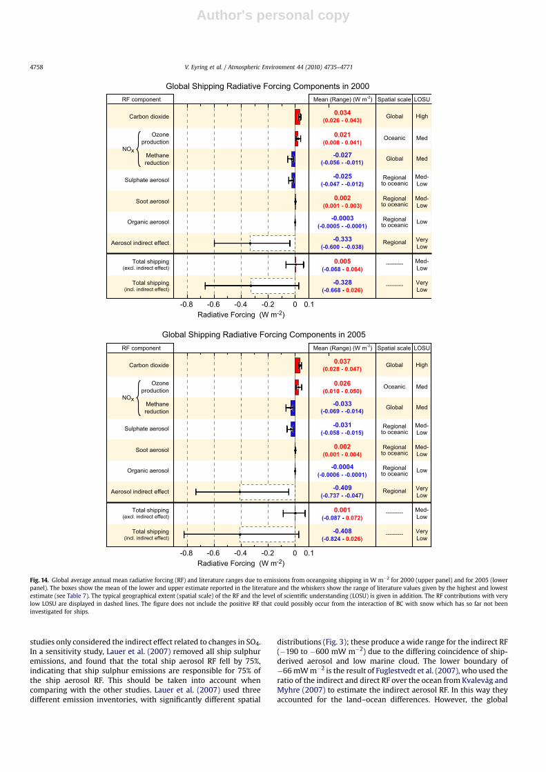
Author's personal copy
studies only considered the indirect effect related to changes in SO4.In a sensitivity study, Lauer et al. (2007) removed all ship sulphuremissions, and found that the total ship aerosol RF fell by 75%,indicating that ship sulphur emissions are responsible for 75% ofthe ship aerosol RF. This should be taken into account whencomparing with the other studies. Lauer et al. (2007) used threedifferent emission inventories, with significantly different spatial
distributions (Fig. 3); these produce a wide range for the indirect RF(�190 to �600 mW m�2) due to the differing coincidence of ship-derived aerosol and low marine cloud. The lower boundary of�66 mW m�2 is the result of Fuglestvedt et al. (2007), who used theratio of the indirect and direct RF over the ocean from Kvalevåg andMyhre (2007) to estimate the indirect aerosol RF. In this way theyaccounted for the land–ocean differences. However, the global
Mean (Range) (W m-2) LOSU
Med-Low
High
Med
Low
VeryLow
Med-Low
Spatial scale
Global
Global
Regionalto oceanic
Regional
0.002
-0.025
0.034
-0.027
-0.0003
-0.333
Global Shipping Radiative Forcing Components in 2000
NOxMethanereduction
Soot aerosol
RF component
Sulphate aerosol
Carbon dioxide
Ozoneproduction
Organic aerosol
Aerosol indirect effect
Med0.021 Oceanic
----------
Regionalto oceanic
Regionalto oceanic
(0.026 - 0.043)
(0.008 - 0.041)
(-0.056 - -0.011)
(0.001 - 0.003)
(-0.047 - -0.012)
(-0.0005 - -0.0001)
(-0.600 - -0.038)
Radiative Forcing (W m-2)-0.8 -0.4 -0.2 0 0.1-0.6
Med-Low
Total shipping(excl. indirect effect)
----------0.005
(-0.068 - 0.064)
VeryLow
Total shipping(incl. indirect effect)
-0.328
(-0.668 - 0.026)
Mean (Range) (W m-2) LOSU
Med-Low
High
Med
Low
VeryLow
Med-Low
Spatial scale
Global
Global
Regionalto oceanic
Regional
0.002
-0.031
0.037
-0.033
-0.0004
-0.409
Global Shipping Radiative Forcing Components in 2005
NOxMethanereduction
Soot aerosol
RF component
Sulphate aerosol
Carbon dioxide
Ozoneproduction
Organic aerosol
Aerosol indirect effect
Med0.026 Oceanic
----------
Regionalto oceanic
Regionalto oceanic
(0.028 - 0.047)
(0.010 - 0.050)
(-0.069 - -0.014)
(0.001 - 0.004)
(-0.058 - -0.015)
(-0.0006 - -0.0001)
(-0.737 - -0.047)
Radiative Forcing (W m-2)-0.8 -0.4 -0.2 0 0.1-0.6
Med-Low
Total shipping(excl. indirect effect)
----------0.001
(-0.087 - 0.072)
VeryLow
Total shipping(incl. indirect effect)
-0.408
(-0.824 - 0.026)
Fig. 14. Global average annual mean radiative forcing (RF) and literature ranges due to emissions from oceangoing shipping in W m�2 for 2000 (upper panel) and for 2005 (lowerpanel). The boxes show the mean of the lower and upper estimate reported in the literature and the whiskers show the range of literature values given by the highest and lowestestimate (see Table 7). The typical geographical extent (spatial scale) of the RF and the level of scientific understanding (LOSU) is given in addition. The RF contributions with verylow LOSU are displayed in dashed lines. The figure does not include the positive RF that could possibly occur from the interaction of BC with snow which has so far not beeninvestigated for ships.
V. Eyring et al. / Atmospheric Environment 44 (2010) 4735–47714758

Author's personal copy
model results of Lauer et al. (2007) indicate that a simple scaling ofthe total anthropogenic indirect aerosol RF to the contribution of anindividual source to the total aerosol burden, even if this is doneonly over the ocean, is questionable, because the large values theycalculate mainly stem from those regions where ship emissionscoincide with frequent occurrence of low clouds, which are highlysusceptible to the enhanced aerosol number concentration in anotherwise clean marine environment (Fig. 15). The only other studythat also used a global model to estimate the indirect aerosol effectwas carried out by Capaldo et al. (1999). They estimated the indirectaerosol RF of ship-derived sulphate particles from model studieswithout detailed aerosol microphysics and aerosol–cloud interac-tion, and found a value of �110 mW m�2. As Lauer et al. (2007)considered a wider range of aerosols, and found that sulphatecontributed about 75% to the total ship-derived aerosol RF, theCapaldo et al. (1999) estimate is close to the lowest estimate givenin Lauer et al. (2007). Fuglestvedt et al. (2007) estimate the RF dueto BC emissions from ships at 2.0 � 0.9 mW m�2.
Despite the wide range of RF values reported, all studies agreethat the present-day net RF due to shipping is negative (see Fig. 14),in contrast to, for instance, estimates of RF from aircraft (Sausenet al., 2005). However, none of the studies on RF from shipping sofar investigated the positive RF that could possibly occur from theinteraction of BC with snow (Hansen and Nazarenko, 2004; Hansenet al., 2005; Koch and Hansen, 2005; Flanner et al., 2007). Flanneret al. (2007) applied a snow, ice, and aerosol radiative modelcoupled to a GCM with prognostic aerosol transport and studied theclimate forcing from fossil fuel, biofuel, and biomass-burning BCemissions deposited to snow. They find that global annual meanequilibrium warming resulting from inclusion of BC in snow is0.1–0.15 K depending on the set of present-day emissions used, butthat the annual Arctic warming is significantly larger (0.5–1.6 K).The results indicate that the interaction between snow and BCcould be an important component of the carbon aerosol climateforcing, in particular in the Arctic. A similar positive BC/snowforcing from ships could potentially play a role in the Arctic in thefuture (see Section 7.2).
5.3. Temperature response and other climate metrics
While the present-day radiative forcing of the differentcomponents of the shipping emissions are useful to evaluate theimpact of historical emissions on climate (up until present), theyare not directly useful to evaluate impacts of present and futureemissions on the future climate. As discussed in Fuglestvedt et al.(2010) there is not a unique correct way to do this, but it dependson how the long-term goals of a climate policy are determined. Inthe Kyoto Protocol to the UNFCCC it was decided to use the globalwarming potential with a 100 year time horizon (GWP100) forthis purpose (see Fuglestvedt et al. (2010) for definition anddiscussion of the GWP and other metrics). Recently Shine et al.(2005, 2007) have proposed a new emission metric, the globaltemperature change potential (GTP), that is designed to servea policy consistent with a long-term climate target of con-straining the global mean surface temperature increase belowa threshold (e.g. the EU’s target of keeping it below 2 �C abovepre-industrial levels).
Due to the short-lived nature of many of the key components ofshipping emissions there are several fundamental problems ofapplying global and annual averaged metric values to thesecomponents. However, they can be readily calculated from theglobal model simulations (Endresen et al., 2003; Eyring et al., 2007;Lauer et al., 2007). Table 8 shows the GWP100, GTP20, GTP50, GTP100
and CO2 equivalent emissions for these metrics for the variouscomponents of the ship emissions and the range caused by
uncertainties in emissions and metric values. The time horizon of50 years for the GTP metrics is used as that may be consistent witha time horizon of stabilizing global temperature increase. Details oninput data and how the metrics are calculated are given inFuglestvedt et al. (2010).
Both SO2 and NOx emissions from shipping are found to causecooling. Using the GWP100 metric and including the large indirecteffects on clouds found by Lauer et al. (2007) present-day shipemissions have negative CO2 equivalent emissions. Note that this issupposed to represent an integrated effect between the time ofemissions and the time horizon and does not imply that currentship emissions will have a cooling effect after 100 years. Indeed theCO2 equivalent emissions using the GTP50 metric indicate that after50 years the net effect of current emissions is nearly neutralthrough cancellation of warming by CO2 and cooling by sulphateand NOx (see Fuglestvedt et al. (2010) for further details on trans-port metrics). Berntsen and Fuglestvedt (2008) use a simpleanalytical climate model to calculate the time dependent contri-butions to global mean temperature change for current emissionsfrom the different transport sectors. In the case of shipping theirresults for a 1 year emission pulse are consistent with the resultsfrom simple analysis using GTPs, in that NOx and SO2 contribute tocooling, and that the long-term warming caused by CO2 leads toa net warming after about 35 years.
6. Mitigation
The potential for emission reductions through technologicalimprovements, alternative fuels and ship modifications is signifi-cant (Eyring et al., 2005b; ICCT, 2007). Several technologies andalternative fuels summarized in Section 6.1 could reduce shipemissions for both new and existing engines. Emissions controlstrategies for the shipping fleet have not been widely adopted inthe absence of policy measures, making their ultimate performanceacross the fleet less certain. Policymakers are debating the trade-offbetween regulations that are technology-based (e.g. mandatingemission reduction systems) or performance-based (e.g. requiringa level of control that may be achieved through alternate controlmeasures; see Section 6.2). Another consideration is whether localmitigation policies (e.g. requiring emissions control in ports only)will result in behaviours that also meet regional and global pollu-tion reduction objectives. While current legislation scenarios havealready been discussed in Section 2.3, Section 6.3 assesses howpossible improvements in technology or the use of alternativeenergies and fuels could impact on the future evolution of shipemissions.
6.1. Technology options, alternative fuels and energy
Here we provide a summary on technology options, alternativefuels and energy. More detailed reports, including how the varioustechniques reduce the emission indices and specific fuelconsumption rates can be found in Corbett and Fischbeck (2002),Eyring et al. (2005b), and ICCT (2007).
6.1.1. Reduction of NOx emissionsNOx emissions are directly related to compression-ignition
(diesel) combustion in marine engines. Marine diesel enginesoperate at low revolutions per minute (rpm), and therefore havevery large cylinder volumes with diameters that routinely rangefrom 20 to 90 cm and piston speeds as slow as 7 m per second(m s�1) (Heywood, 1988; Harrington, 1992). Over the past 25 years,the power output per cylinder has more than doubled whilespecific fuel consumption has decreased by 25%, mainly throughincreased maximum firing pressure and better fuel injection
V. Eyring et al. / Atmospheric Environment 44 (2010) 4735–4771 4759

Author's personal copy
control, supercharging, and scavenging (Heywood, 1988). To beefficient, the fuel injected into large cylinders has to atomize and bewell mixed with air before the long-duration power strokes. Thiscombustion leads to higher peak temperatures and longer resi-dence times, which cause marine engines to have typically higherNOx emissions than other diesel engines (Carlton et al., 1995). TheNOx resulting from nitrogen bound in the heavy residual fuel usedby oceangoing ships can also lead to higher NOx emissions.
Technologies that reduce NOx emissions can be divided intothree groups (MAN B&W, 1996; European Commission and EntecUK Limited, 2005): those that require engine modifications (inengine controls), those that are implemented in the fuel or airsystem (pre-engine technologies), and those that are on theexhaust system (post-engine technologies). Pre-Engine technolo-gies, e.g. include the addition of water to the diesel combustionprocess, which is a promising approach to reduce emissions,primarily NOx. Any method of introducing water into thecombustion space reduces the formation of NOx by cuttingtemperature peaks in the engine cylinder. Techniques under thiscategory include fuel water emulsification (FWE), humid air motor(HAM), and combustion air saturation system (CASS). In engine NOx
control strategies include aftercooler upgrades, engine derating,injection timing delays, fuel system modifications to increasesupply pressure, diesel-electric propulsion and marine gas turbinepropulsion. Post-engine technologies, e.g. include the selectivecatalytic reduction (SCR) for NOx controls.
6.1.2. Reduction of SOx and particulate matter emissionsSOx emissions from ships are important precursors for aerosols
and are determined by the sulphur content of the fuel. The mosteffective measure to reduce SOx and particulate matter emissionsfrom ships therefore is to lower the sulphur content in marine fuels.Due to predicted low sulphur fuel supply limitations and the highprice premium of low sulphur marine fuel other options areconsidered. The scrubber option is receiving increasing attention asa cost-effective alternative (European Commission and Entec UKLimited, 2005). Due to seawater’s natural alkalinity and the largequantities of sulphur already in it, seawater scrubbing is a versatile,readily available and cost-effective process. SO2 reduction rates byseawater scrubber demonstrations show similar SO2 reductionrates (between 65 and 94%) with 75–80% being sustainably ach-ieved when operating the system within the existing designparameters. A diesel particulate filter system in the exhaust streamcollects and stores particles, usually equipped with a means to burnoff accumulated particulate with or without catalysts. Rated effi-ciencies in service with on-road distillate fuels range from 80% tomore than 90% control of PM. The diesel oxidation catalyst (DOC) isdesigned to convert particulate matter that contains liquid hydro-carbons or soluble organic fractions through post-combustionoxidation. The reduction in overall PM emissions with a DOC isa function of the fraction of total PM that can be oxidized, generally20–50% using on-road diesel fuels, probably 10–30% in marineapplications.
Fig. 15. Multi-year average of simulated changes in shortwave cloud forcing due to shipping at the top of the atmosphere (ToA) in W m�2. Upper row shows the geographicaldistribution, lower row zonal averages. Hatched areas (upper row) and light-red shaded areas (lower row) show differences which are significant at the 99% confidence levelcompared to the inter-annual variability (from Lauer et al., 2007, their Fig. 11).
Table 8Emission metrics (GWP100, GTP20, GTP50, GTP100) and corresponding CO2 equivalent emissions (in Tg (CO2)/year for all metrics) for the various components of ship emissions.The range in the brackets represent the range caused by uncertainties in emissions and metric values. The metric values for SO2 is given on SO2 basis, while for NOx it is given onN-basis (cf. Fuglestvedt et al., 2010). Ranges for CO2 emissions are taken from Table 7.
GWP100 GTP20 GTP50 GTP100 CO2-eq emissions(GWP100-based)
CO2-eq emissions(GTP20-based)
CO2-eq emissions(GTP50-based)
CO2-eq emissions(GTP100-based)
CO2 1 1 1 1 [501, 812] [501, 812] [501, 812] [501, 812]SO2 (direct) [�43, �11] [�44, �11] [�7.3, �1.8] [�6.1, �1.5] [�520, �75] [�530, �75] [�88, �12] [�73, �10]SO2 (total) [�480, �230] [�380, �180] [�63, �30] [�53, �25] [�5800, �1600] [�4600, �1200] [�760, �200] [�640, �170]NOx [�36, �25] [�190, �130] [�35, �30] [�6.1, �4.2] [�230, �73] [�1240, �380] [�230, �87] [�40, �12]
V. Eyring et al. / Atmospheric Environment 44 (2010) 4735–47714760

Author's personal copy
6.1.3. Alternative fuelsThere are a number of alternative fuels that can be used in
marine service (National Research Council, 1980). Primary fuelsources are fossil fuels, petroleum, goal, and gas. Fuels derived frompetroleum are commonly considered alternate marine fuels toheavy residual oil (marine bunkers). These include low sulphurresidual fuels, marine distillates and blends (ISO, 1987). Coal-derived and gaseous fuels can be used in marine engines. Gaseousfuels can also be used in marine internal combustion engines (ICEs).The use of hydrogen diesel in large-bore diesel engines has beendeveloped for high power densities and low exhaust gas emissions(Vogel, 1999). NOx is the only pollutant of such an engine, butslightly more is produced than with marine distillate oil (MDO) orheavy fuel oil (HFO). This means NOx reduction methods have to beapplied, which, due to the relatively clean exhaust gas, work moreefficiently. CO2 is less than 2% of the CO2 emission of a conventionaldiesel engine.
Bio-oils, such as palm oil, coconut oil, rapeseed oil, soya oil andothers have been suggested as fuel for small low power combustionengines for many years. Within the last few years, the first testswith biofuels have been made with land-based medium-speeddiesel engines in the power range of several MW, and the first fewcommercial biofuel engines have been sold already by manufac-turers (Gros, 2002). Bio-diesel, defined as the mono alkyl esters oflong-chain fatty acids derived from renewable lipid sources, offersome potential to reduce particulate matter and are being evalu-ated for their potential to reduce CO2 emissions on a life-cycle basis(including carbon uptake during plant growth). However, only inrecent years have bio-diesel gained commercial attention,primarily in land-based installations.
However, efforts to introduce alternative fuels in marine vesselshave raised questions about the energy use and environmentalimpacts of such fuels. Understanding the true emissions frommarine transportation requires a total fuel cycle analysis (TFCA).TFCA involves consideration of energy use and emissions from theextraction of raw fuel (e.g. oil from the ground) to the use of theprocessed fuel in the vessel itself. Each stage in the fuel cycleincludes activities that produce GHG and criteria pollutant emis-sions. These emissions are typically caused by fuel combustionduring a particular stage, although some non-combustion emis-sions occur (e.g. natural gas emissions from pipeline leaks, evapo-rative losses in refueling). The goal of a TFCA is to account for eachof the emissions events along the entire fuel cycle. One approach tocompare these multistage energy and emissions for ships is theTotal Energy & Emissions Analysis for Marine Systems (TEAMS)model (Winebrake et al., 2007; Corbett and Winebrake, 2008).TEAMS captures ‘‘well-to-hull’’ emissionsdthat is, emissions alongthe entire fuel pathway, including extraction, processing, distribu-tion, and use in vessels. TEAMS produces emissions estimatesdirectly, not full impacts analyses; however, emissions estimated byTEAMS (or similar tools that are not intrinsically geospatial) atvarious stages in the fuel cycle can be geographically located,allowing impacts to be evaluated according to local environmentalor social conditions.
6.1.4. Reduction of fuel consumption and CO2
Optimization of various ship systems other than the enginessuch as propeller, rudder, and hull are promising options to reducefuel consumption rates and, with them, GHG emissions (Maedaet al., 1998). The energy-reduction potential, and therefore theemission reduction potential, of an optimized hull shape anda better propeller for a new ship are estimated to be up to 30%(MARINTEK, 2000). Proper ship maintenance can ensure that thevessel operates efficiently (ICCT, 2007). The most effective way toreduce fuel consumption and GHG emissions from ships is reducing
and optimizing the vessel speed and adjust ship routes to avoidheavy wind (Skjølsvik et al., 2000).
In addition, alternative power systems or the combination ofthose with the traditional ship energy source could reduce GHGemissions from ships. A few commercial installations of fuel cells(FC) onboard very small ships are currently in use. Wind can beused as propellant for ships in two ways, as a power producer bywind turbines or as a thruster producer by sails or similar devices.Solar cells, as fuel cells, are the type of prime movers that produceenergy without torque. They deliver voltage and the electricalcurrent drives the motor which in turn drives the propeller ofa ship. The advantages are no fuel consumption and no emission(Ahlqvist, 1999). Although already in use today for demonstrationpurposes on a few small boats, the disadvantage of solar panelstoday is their enormous price level and their size in order to providean appropriate power density, but ongoing research and develop-ment might change this situation.
6.2. Policy strategies
Future emissions are influenced by the application of emissioncontrol measures. The maritime industry is at the centre of inter-national attention due to increasing pressure to reduce emissionsfrom marine vessels and port operations. Policymakers respondedto these concerns by considering emissions reduction programsspecifically for vessel and port activities. Policy instruments forachieving environmental objectives can be categorized intocommand-and-control approaches and market-based or incentive-based approaches. Policy measures to reduce ship emissions arebriefly discussed here and detailed in Cofala et al. (2007) and ICCT(2007).
Command-and-control regulations achieve environmentalmanagement goals by setting uniform standards for sources ofpollutants (Stavins, 2002). In market-based approaches, policymakers use market signals and economic incentives to encouragedesired behaviour (Seik, 1996; Stavins, 2002; UNEP, 2002). Theseapproaches are defined broadly by the U.S. EPA as instruments thatuse financial means to motivate polluters to reduce the health andenvironmental risks posed by their facilities, processes, or products(U.S. Environmental Protection Agency, 2001). There have beenseveral studies conducted to evaluate the cost-effectiveness ofdifferent approaches for reducing ship emissions (Farrell et al.,2003; Kågeson, 1999; Swedish Shipowners’ Association, 2002).These studies have largely argued that the regulatory approach onthe shipping industry had not been very successful until 2002(Swedish Shipowners’ Association, 2002). In particular, there wasno incentive for ships to invest in pollution control equipment –shipowners who invested in environmentally friendly equipmentwere at an economic disadvantage compared to those who didnothing (Volk et al., 2000). But now a number of direct and indirectincentives that support emissions reduction on ships are available(Coalition Clean Baltic et al., 2001; Volk et al., 2000). There arevarious types of regulatory instruments considered command-and-control, and the most prevalent regulatory instruments are tech-nology and performance-based standards (Stavins, 2002). Tech-nology-based standards specify the method, and sometimes theactual equipment, that firms must use to comply with a particularregulation. A performance-based standard sets a uniform controltarget for firms, while allowing some latitude in how this target ismet. For example, the MARPOL Annex VI SECA requirements can becategorized as a performance-based regulation because ships caneither switch to low sulphur fuel or use approved technology toreduce an equivalent amount of SO2 emissions.
Market-based instruments encompass a range of policy toolsfrom pollution taxes, charges, to marketable permits, to
V. Eyring et al. / Atmospheric Environment 44 (2010) 4735–4771 4761

Author's personal copy
government subsidies – all of which change poor environmentalbehaviour by changing the incentive structure for polluters (Pan-ayotou, 1994; Stavins, 2002; UNEP, 2002). If well designed andimplemented, market-based instruments have the potential to bemore cost-effective than command-and-control regulations,because command-and-control measures set emissions targets/limits for which cost-reducing measures apply where economicinstruments often incentivize both cost-reducing and emissionsreducing innovations (Harrington and Morgenstern, 2004).Economic incentives can also encourage polluters to controlpollution above and beyond the level required by regulation, aswell as spur technological innovation for pollution control tech-nologies. Market-based instruments, e.g. include environmentaldifferentiation of fairway and port fees, ship environment indexsystem and differentiated tonnage tax (green tax), the green awardfoundation (GAF), and emission trading. Overall, there is increasingsupport for market-based instruments. For example, Europe iscurrently discussing whether shipping is going to be included intothe EU emission trading scheme (EU ETS).
6.3. Assessment of mitigation scenarios
In coming decades, newly introduced policy measures couldmodify an unconstrained growth trend in energy use. In terms oftechnology, there could be further improvements in thermal effi-ciency, fuel type and quality, and propulsion design. Currentinternational legislation scenarios have already been discussed inSection 2.3. Here we show how possible improvements in tech-nology or the use of alternative energies and fuels could impact onthe future evolution of ship emissions.
The vast majority of marine propulsion and auxiliary plantsonboard oceangoing ships are diesel engines. In terms of themaximum installed engine output of all civilian ships above 100GT, 96% of this energy is produced by diesel power. These enginestypically have lifetimes of 30 years and more. Because of missingalternative propulsion systems with similar power density, primecosts and fuel efficiency, it is expected that diesel engines willnot be replaced in the foreseeable future. Therefore, at least fora mid-term period (around 20 years), emission reduction ofexisting engines will be based on effective emission reductiontechnologies or changes in the fuel. On the other hand, it is hardto assess which of the alternative techniques or fuels discussed inSection 6.1 are likely to be in use on the long-term, for examplein 2050. However, keeping in mind that the world’s oil reservesare limited (British Petrol, 2004) and that first tests with alter-native fuels and energies are already underway, a shift froma diesel-only fleet to a fleet that partly uses alternative fuels andenergies in 2050 is likely.
Based on these assumptions, Eyring et al. (2005b) presented 16emission scenarios through 2050 obtained by a mid-term prog-nosis for 2020 and a long-term prognosis for 2050. The scenariosare a combination of four future ship traffic demand scenarios andfour technology scenarios. The future ship traffic demandscenarios are mainly determined by the economic growth, whichfollows the IPCC SRES storylines (see Section 2.3). The resultingfuel consumption is projected through extrapolations of historicaltrends in economic growth, total seaborne trade and number ofships, as well as the average installed power per ship. For thefuture technology scenarios they assume a diesel-only fleet in2020 resulting in fuel consumption between 382 and 409 Mt. For2050 one technology scenario assumes that 25% of the fuelconsumed by a diesel-only fleet can be saved by applying futurealternative propulsion plants, resulting in a fuel consumption thatvaries between 402 and 543 Mt. The other scenario is a business-as-usual scenario for a diesel-only fleet even in 2050 and gives an
estimate between 536 and 725 Mt. Dependent on how rapidtechnology improvements for diesel engines are introduced,possible technology reduction factors are applied to the today’sfleet-average emission factors. The study showed that future totalship emissions, especially NOx and SOx emissions will be mainlydetermined by the technology and to a lesser extent by the futureglobal economic development. In future scenarios this means thatthe calculated total emissions are dominated by the chosentechnology reduction rates, and to a lesser extent by the assumedannual growth in GDP and the factor by which the fuelconsumption of a diesel-only fleet in 2050 is saved throughapplication of alternative energies and fuels. With aggressive NOx
reduction, a significant decrease from 6.52 Tg(N) in 2001 to0.94 Tg(N) could be reached by 2050, despite a growing fleet (seeFig. 6). On the other hand, if no further reduction techniques areapplied and future diesel engines will be equipped with tech-niques that fulfil the current IMO regulations, a further significantincrease has to be expected until 2050. Future SOx emissions willmainly be determined by the sulphur content of the fuel. In theirclean scenario they assumed an average sulphur content of 1% in2020 and 0.5% in 2050, compared to 2.4% today. This reduces SOx
emissions from 6.0 Tg (SO2) in 2001 to 1.8 Tg(S) by 2050. FutureCO2 emissions in these scenarios are on the other hand mainlydetermined by the total fuel consumption, which in turn is mainlydetermined by the economic growth and the amount of the fuelconsumption that is saved by alternative energies and fuels. Theestimates suggest CO2 emissions between 1110 and 1188 Tg (CO2)in 2020 and between 1109 and 2001 Tg (CO2) in 2050.
Cofala et al. (2007) used the European Monitoring and EvaluationProgramme (EMEP) model to run a base year 2000 and 240 emissioncontrol cases for the year 2020. The baseline scenario in 2020outlines the effects of current legislation on emissions from shipping.At the other end the Maximum technically feasible reductions (MFR)scenario quantifies emissions, environmental effects and costs ofimplementing the best available control technology on internationalshipping. Between the baseline and the MFR scenario, differentambition level scenarios are presented. For example, the Ambitionlevel 2 scenario assumes a sulphur content of 0.5% in residual oil orscrubbing equivalent (2 g SO2/kWh) in SECA, and for passengervessels everywhere. Regarding NOx emissions, it is assumed thatHAM for all new engines post-2010 are installed. Compared to 2000,emissions of SO2 from international shipping are expected toincrease till 2020 in the baseline scenario by 42%, and NOx and PM2.5
emissions by 47% and 55%, respectively. This growth is mainlyrelated to the assumed increase in traffic volume, while the addi-tional emission control measures that are considered in the baseline(i.e. sulphur controls according to the EU Marine Fuel Directive,MARPOL standards on new vessels) show only limited impact.Maximum technically feasible emission reductions would declineSO2 and NOx emissions by 78 and 89%, respectively. As a side effect ofusing low sulphur fuel, emissions of PM decrease by 15% comparedwith the baseline.
Dalsøren et al. (2007) complemented existing global sea trans-portation emission inventories with new regional emission data-sets and scenarios for ship traffic and coastal activity in 2015. Thescenarios adopted for 2015 assumed 2% yearly increase in bunkerfuel consumption for the existing (year 2000) global fleet, but tookinto account potential reductions in emissions of componentsregulated by ANNEX VI of MARPOL (e.g. assumed only 15% increase2000–2015). In the SECA of the North Sea and the Channel it wasassumed that the ships adhered to the ANNEX VI demandinga maximum sulphur content of fuel oil of 1.5%. Assuming nochanges in other emissions, the increases in sea transportationresulted in more than 20% increase in NO2 from 2000 to 2015 insome coastal areas.
V. Eyring et al. / Atmospheric Environment 44 (2010) 4735–47714762
Author's personal copy
All these scenario calculations show that ship emissions shouldbe recognized as a growing problem for scientists, industry andenvironmental policy makers. Currently ship emissions are one ofthe least regulated sources of anthropogenic emissions with a highreduction potential through technological improvements, alterna-tive fuels and ship modifications. The scenario calculations furtherdemonstrate that significant reductions are needed to offsetincreased emissions due to growth in seaborne trade.
7. Future impacts on atmospheric composition and climate
Most studies that are available on possible atmospheric andclimate impacts in the future focused on current legislation andsome emission control scenarios in the nearer future (Section 7.1).Some studies also provided projections of impacts under theassumption of changing shipping patterns due to climate change(Section 7.2).
7.1. Projected changes for current legislation and emissioncontrol scenarios
The efficiency of ozone production from NOx emissionsdecreases with increasing background NOx concentration and withthe magnitude of the emissions (e.g. Lin et al., 1988). Thus theimpact of shipping might be expected to depend on the land-basedemission scenario chosen. This was investigated by Collins et al.(2009) who found that the shipping contribution (at 2000 shippinglevels) to European surface ozone in 2030 varied from 1.1 ppb withthe highest land-based emissions (2030 SRES A2) to 2.6 ppb withthe lowest land-based emissions (2030 IIASA MFR). The MFRscenario considers the scope for emission reductions offered by fullimplementation of the presently available emission control tech-nologies, while maintaining the projected levels of anthropogenicactivities. Similarly the effect of shipping on the global troposphericozone budget is smallest for the A2 land-based scenario and largestfor the MFR (Fig. 16). This figure also shows a small decrease inozone production efficiency with increasing magnitude of shipemissions, confirming earlier findings by Eyring et al. (2007). Whilethe future level of shipping NOx emissions is very uncertain (seescenario calculations in Fig. 6), a constant growth in shipping wouldoffset some of the expected benefits in surface ozone pollutionfrom land-based emission control legislation.
The effects of NOx emissions on the OH concentrations, andhence methane lifetimes, are expected to be non-linear as wasfound for the ozone. Fig. 16 shows that the change in methanelifetime is largest when the land-based emissions are smallest(MFR), and that the change is less than linear in the ship NOx
emissions. Again, this confirms similar findings in Eyring et al.(2007).
Eyring et al. (2007) showed that under the assumption ofa constant annual growth rate for ship emissions of 2.2% per year upto 2030 (CGS), shipping would significantly counteract the benefitsderived from reducing SO2 emissions from all other anthropogenicsources under the IPCC SRES A2 scenario over the continents by2030, for example in Europe. Globally, shipping contributes 4.5% toincreases in sulphate under A2/CGS until 2030. However, if futureland-based emissions follow a more stringent scenario, the relativeimportance of ship emissions will be even higher. Using a futurescenario for both land-based and shipping emissions in 2015 Dal-søren et al. (2007) found that the SO2 concentrations increased lessthan linearly due to the increased oxidants.
The EMEP model simulations by Cofala et al. (2007) suggest that,at present, emissions from ships are responsible for 10–20% ofsulphur deposition in coastal areas over Europe (see Fig. 17). Until2020 their contribution is expected to increase to more than 30% in
large areas along the coast in Europe in the baseline scenario. Inmany coastal areas, ships will be responsible for more than 50% ofsulphur deposition. Emission controls on shipping will bring downthe depositions to much lower levels.
7.2. Projected changes in shipping patterns
Emissions from shipping and fisheries may change due toclimate change. Mostly studied is the potential opening of theNorthern Sea Route (NSR) via the Barents Sea between Europe andthe north Pacific Region, but also sea level rise and changes in thelocation and amounts of fish stocks may be of some importance. Fornone of these climate induced changes there has yet been estab-lished well founded emission scenarios.
The Arctic is now experiencing some of the most rapid climatechanges on Earth. On average, the rate of temperature increasehas been twice as high as for the rest of the world. Observationsover the past 50 years show a decline in Arctic sea-ice extentthroughout the year, with the most prominent retreat in summer.The melting of Arctic sea-ice will effectively unlock the ArcticOcean area, leaving it increasingly open to human activity –particularly shipping and oil/gas production (IPCC, 2007; Serrezeet al., 2007).
The trends indicate an Arctic Ocean with longer seasons of lesssea-ice cover of reduced thickness, implying improved ship acces-sibility around the margins of the Arctic Basin. Climate modelsproject an acceleration of this trend and opening of new shippingroutes and extension of the period during which shipping isfeasible. The seaborne cargo transport in these waters has previ-ously been very limited, and the reported ship emissions low(PAME, 2000; Corbett et al., 1999; Endresen et al., 2003). The travelalong the NSR can reduce travel time by up to 50%, compared to searoutes travelled today (Fritjof Nansen Institute, 2000). Thus, if thenumber of navigation days increases it is expected that more trafficwill pass along this route.
It is expected that increased shipping traffic will result inincreased air pollution burden in this area (AMAP, 2006) andchanges in regional climate forcing. Granier et al. (2006) have useda global chemical tracer model, assuming that up to 11% of totalship emissions will occur in the Arctic. They find that the Arctic mayexperience summer concentrations of ozone two to three times thecurrent value and comparable with those seen in many industri-alized regions in the Northern hemisphere. On the other hand thechange in ship routes may imply less shipping transport globallysince the new routes are shorter, thus the new routes may implya shift in emissions from other locations and saved fuel (and lessemissions) for the same amount of goods transported, and conse-quently influencing long-range transport of air pollution. However,this also means that emissions may be shifted from less vulnerableregions to the Arctic. Increased air pollution and deposition in theArctic is of particular concern because of the high vulnerability, andin the case of soot deposition as a climate feedback mechanism(Flanner et al., 2007).
Dalsøren et al. (2007) included estimates and developedinventories for expected new regional emissions not previouslyquantified. These additional datasets were found to be of signif-icant importance for environmental assessments and the CTMresults in northern regions. By 2015, more than 1500 tankers mayexport oil via the Barents Sea and the Northeast Atlantic toEurope and the US. Increased oil and gas export from theNorwegian sector is also likely and gas power plants are plannedalong the Norwegian coast. The NSR for international transitshipping operations to Asia today is limited but could becomemore important if infrastructure develops and if the ice thicknessand coverage decrease due to regional warming. In 2015 the
V. Eyring et al. / Atmospheric Environment 44 (2010) 4735–4771 4763
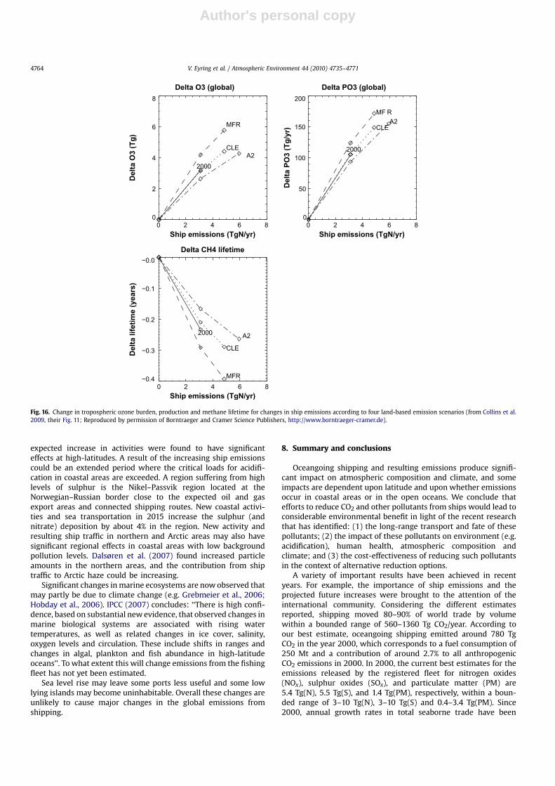
Author's personal copy
expected increase in activities were found to have significanteffects at high-latitudes. A result of the increasing ship emissionscould be an extended period where the critical loads for acidifi-cation in coastal areas are exceeded. A region suffering from highlevels of sulphur is the Nikel–Passvik region located at theNorwegian–Russian border close to the expected oil and gasexport areas and connected shipping routes. New coastal activi-ties and sea transportation in 2015 increase the sulphur (andnitrate) deposition by about 4% in the region. New activity andresulting ship traffic in northern and Arctic areas may also havesignificant regional effects in coastal areas with low backgroundpollution levels. Dalsøren et al. (2007) found increased particleamounts in the northern areas, and the contribution from shiptraffic to Arctic haze could be increasing.
Significant changes in marine ecosystems are now observed thatmay partly be due to climate change (e.g. Grebmeier et al., 2006;Hobday et al., 2006). IPCC (2007) concludes: ‘‘There is high confi-dence, based on substantial new evidence, that observed changes inmarine biological systems are associated with rising watertemperatures, as well as related changes in ice cover, salinity,oxygen levels and circulation. These include shifts in ranges andchanges in algal, plankton and fish abundance in high-latitudeoceans’’. To what extent this will change emissions from the fishingfleet has not yet been estimated.
Sea level rise may leave some ports less useful and some lowlying islands may become uninhabitable. Overall these changes areunlikely to cause major changes in the global emissions fromshipping.
8. Summary and conclusions
Oceangoing shipping and resulting emissions produce signifi-cant impact on atmospheric composition and climate, and someimpacts are dependent upon latitude and upon whether emissionsoccur in coastal areas or in the open oceans. We conclude thatefforts to reduce CO2 and other pollutants from ships would lead toconsiderable environmental benefit in light of the recent researchthat has identified: (1) the long-range transport and fate of thesepollutants; (2) the impact of these pollutants on environment (e.g.acidification), human health, atmospheric composition andclimate; and (3) the cost-effectiveness of reducing such pollutantsin the context of alternative reduction options.
A variety of important results have been achieved in recentyears. For example, the importance of ship emissions and theprojected future increases were brought to the attention of theinternational community. Considering the different estimatesreported, shipping moved 80–90% of world trade by volumewithin a bounded range of 560–1360 Tg CO2/year. According toour best estimate, oceangoing shipping emitted around 780 TgCO2 in the year 2000, which corresponds to a fuel consumption of250 Mt and a contribution of around 2.7% to all anthropogenicCO2 emissions in 2000. In 2000, the current best estimates for theemissions released by the registered fleet for nitrogen oxides(NOx), sulphur oxides (SOx), and particulate matter (PM) are5.4 Tg(N), 5.5 Tg(S), and 1.4 Tg(PM), respectively, within a boun-ded range of 3–10 Tg(N), 3–10 Tg(S) and 0.4–3.4 Tg(PM). Since2000, annual growth rates in total seaborne trade have been
Delta O3 (global)
0 2 4 6 8Ship emissions (TgN/yr)
0
2
4
6
8
Delta O
3 (T
g)
2000
MFR
CLEA2
Delta PO3 (global)
0 2 4 6 8Ship emissions (TgN/yr)
0
50
100
150
200
Delta P
O3 (T
g/yr)
2000
MF R
CLEA2
Delta CH4 lifetime
0 2 4 6 8Ship emissions (TgN/yr)
−0.4
−0.3
−0.2
−0.1
−0.0
Delta lifetim
e (years)
2000
MFR
CLE
A2
Fig. 16. Change in tropospheric ozone burden, production and methane lifetime for changes in ship emissions according to four land-based emission scenarios (from Collins et al.2009, their Fig. 11; Reproduced by permission of Borntraeger and Cramer Science Publishers, http://www.borntraeger-cramer.de).
V. Eyring et al. / Atmospheric Environment 44 (2010) 4735–47714764
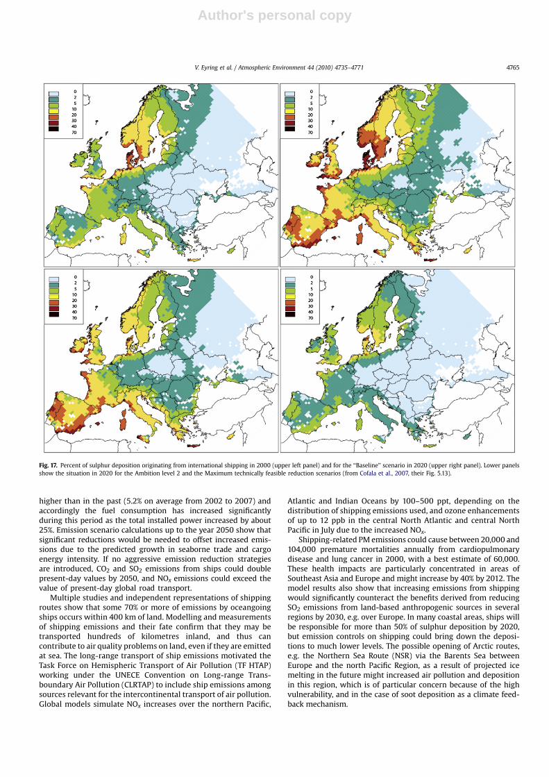
Author's personal copy
higher than in the past (5.2% on average from 2002 to 2007) andaccordingly the fuel consumption has increased significantlyduring this period as the total installed power increased by about25%. Emission scenario calculations up to the year 2050 show thatsignificant reductions would be needed to offset increased emis-sions due to the predicted growth in seaborne trade and cargoenergy intensity. If no aggressive emission reduction strategiesare introduced, CO2 and SO2 emissions from ships could doublepresent-day values by 2050, and NOx emissions could exceed thevalue of present-day global road transport.
Multiple studies and independent representations of shippingroutes show that some 70% or more of emissions by oceangoingships occurs within 400 km of land. Modelling and measurementsof shipping emissions and their fate confirm that they may betransported hundreds of kilometres inland, and thus cancontribute to air quality problems on land, even if they are emittedat sea. The long-range transport of ship emissions motivated theTask Force on Hemispheric Transport of Air Pollution (TF HTAP)working under the UNECE Convention on Long-range Trans-boundary Air Pollution (CLRTAP) to include ship emissions amongsources relevant for the intercontinental transport of air pollution.Global models simulate NOx increases over the northern Pacific,
Atlantic and Indian Oceans by 100–500 ppt, depending on thedistribution of shipping emissions used, and ozone enhancementsof up to 12 ppb in the central North Atlantic and central NorthPacific in July due to the increased NOx.
Shipping-related PM emissions could cause between 20,000 and104,000 premature mortalities annually from cardiopulmonarydisease and lung cancer in 2000, with a best estimate of 60,000.These health impacts are particularly concentrated in areas ofSoutheast Asia and Europe and might increase by 40% by 2012. Themodel results also show that increasing emissions from shippingwould significantly counteract the benefits derived from reducingSO2 emissions from land-based anthropogenic sources in severalregions by 2030, e.g. over Europe. In many coastal areas, ships willbe responsible for more than 50% of sulphur deposition by 2020,but emission controls on shipping could bring down the deposi-tions to much lower levels. The possible opening of Arctic routes,e.g. the Northern Sea Route (NSR) via the Barents Sea betweenEurope and the north Pacific Region, as a result of projected icemelting in the future might increased air pollution and depositionin this region, which is of particular concern because of the highvulnerability, and in the case of soot deposition as a climate feed-back mechanism.
Fig. 17. Percent of sulphur deposition originating from international shipping in 2000 (upper left panel) and for the ‘‘Baseline’’ scenario in 2020 (upper right panel). Lower panelsshow the situation in 2020 for the Ambition level 2 and the Maximum technically feasible reduction scenarios (from Cofala et al., 2007, their Fig. 5.13).
V. Eyring et al. / Atmospheric Environment 44 (2010) 4735–4771 4765

Author's personal copy
In addition to the impact on atmospheric composition andhuman health, ship emissions have an impact on climate. For someof the compounds emitted from ships the radiative forcing (RF) ispositive (CO2, O3 and BC) while for others the forcing is negative(direct effect of sulphate particles, reduced methane). The particlescan also have an indirect effect on climate through their abilitymodify the optical properties of clouds by acting as cloudcondensation nuclei (CCN) or by dissolving in the cloud drops andso change their surface tension. Of all anthropogenic sources, ship-stack effluents provide the clearest demonstration of the indirectaerosol effect on cloud albedo. Curves of larger reflectance in cloudfields, so called ship tracks, can be observed in satellite imagery asa recurrent phenomenon. One of the major findings in terms ofclimate impact was that particle emissions and their precursorsfrom shipping can significantly modify the microphysical andoptical properties of clouds (the so called ‘‘indirect aerosol effect’’).Although the associated uncertainties are still high, the modelresults indicate that the cooling due to altered clouds far outweighsthe warming effects from greenhouse gases such as carbon dioxide(CO2) or ozone from shipping, overall causing a negative radiativeforcing today. The indirect aerosol effect of ships on climate is foundto be far larger than previously estimated contributing between 17and 39% to the total indirect effect of anthropogenic aerosols,depending on the ship emission inventory used. This contributionis high because ship emissions are released in regions with frequentlow marine clouds in an otherwise clean environment and thepotential impact of particulate matter on the radiation budget islarger over the dark ocean surface than in polluted regions overland. Despite the wide range of RF values reported in differentinvestigations, all studies agree that the present-day net RF due toshipping is negative, in contrast to, for instance, estimates of RFfrom aircraft. However, none of the studies on RF from shipping sofar investigated the positive RF that could possibly occur from theinteraction of BC with snow.
As this new research has indicated, reductions in sulphuremissions could result in regional reductions in its resultantnegative radiative forcing. The climatic trade-off between positiveand negative radiative forcing is still a topic of scientific research,but from what is currently known, a simple cancellation of globalmeans is potentially inappropriate and a more comprehensiveassessment metric is required. We emphasize, however, that CO2
remains in the atmosphere for a long-time and will continue tohave a warming effect long after its emission. In contrast, sulphatehas a residence time in the atmosphere of approximately 10 days,and the climate response from sulphate is of the order decadeswhilst that of CO2 is of the order of centuries. Indeed the CO2
equivalent emissions using the global temperature change poten-tial (GTP) metric indicate that after 50 years the net effect of currentemissions is nearly neutral through cancellation of warming by CO2
and cooling by sulphate and NOx. While the control of NOx, SO2 andparticle emissions from ships will have beneficial impacts on airquality, acidification and eutrophication, CO2 reductions from allsources, including ships and other freight modes, will give thegreatest long-term reduction in global warming.
Further work is needed to reach a complete synthesis of theimpact of shipping on atmospheric composition and climate.Uncertainties in the simulated ozone contributions from ships withdifferent model approaches are found to be significantly smallerthan estimated uncertainties stemming from the ship emissioninventory and the neglect of plume processes. This reflects that thenet ozone change from ship emissions under relatively cleanconditions in global models is rather similar and suggests that theatmospheric models are suitable tools to study these effects.However, there is considerable uncertainty in the ship emissioninventories, which has to be further explored. One approach is to
develop bottom-up inventories based on ship movement data andcompare them with activity-based top-down approaches. Bothemission totals and the geographical distribution are key parame-ters for the simulation of atmospheric impacts. The large differ-ences in model results obtained with different ship emissioninventories imply a high uncertainty in the input data.
From the point of view of large-scale composition impacts, thereis not enough observational data to confirm or refute the variousemission datasets used by global models. There are sound chemicalreasons why spreading shipping plumes over the size of gridsquares used by global models could overestimate the NOx, OH andozone responses. Plume model studies have not provided a simplereduction factor for the NOx emissions that could be applied toglobal models. The step from case studies to a suitable parame-terisation of subgrid-scale processes in global models has to bemade for both gaseous and particulate emissions. To reach this,more measurements and model studies are needed to understandplume processes. Additional in situ measurements inside singleship plumes, but also in the corridor of the shipping lanes arerequired for different regions of the world to evaluate the globalmodels’ response to ship emissions. Unambiguous detection of NOx
emissions from ships in satellite data is currently only available forthe region of the Red Sea and the Indian Ocean where shippingroutes are close to the coastal area. Reduction in measurementuncertainties through use of long-term averages and data frommore instruments (e.g. OMI and GOME-2) combined with betterconstraints on land-based sources and higher spatial resolution inthe models should facilitate such an intercomparison in the future.The model studies also need to include different approaches thanthe ones applied so far. More work is needed on the thermody-namical parameters in the marine boundary layer (MBL) thatcontrol transport of ship effluent into the cloud layer, includinglarge eddy simulations of the MBL stability, ship track buoyancyaffected by fuel burning, and subcloud saturation conditions.
Current uncertainties of global modelling studies on the effectsof emissions from shipping on aerosols and clouds are expected tobe much higher than in the case of the ozone change studies. Inparticular the indirect aerosol effect depends crucially on simulatedkey properties such as the aerosol size-distribution and the acti-vation of aerosol particles in clouds. Minor changes of theseproperties can have a significant impact on the simulated indirecteffect. Furthermore, changes in cloud properties such as cloudliquid water content, cloud cover and precipitation due to shipemissions impact on atmospheric chemistry via wet deposition andchanges in scavenging efficiency. Changes in atmospheric chem-istry, e.g. ozone and OH concentrations, may result in a feedback onaerosols, e.g. via modified oxidation rates of SO2. Further modeldevelopment in particular on the representation of aerosol size-distribution, aerosol activation, aerosol–cloud interaction andextension of feedback mechanisms is needed in addition toextended measurement data, e.g. of the size-distribution andcomposition of particles emitted by ships to reduce currentuncertainties in global model studies.
Despite the uncertainties discussed above, with respect to localpollutants such as particulate matter and sulphur emissions,mounting evidence shows that the benefits of emission reductionsof these pollutants outweigh the costs of control for many regionsof the globe. The net benefit of policy action to reduce ship emis-sions has been convincingly demonstrated, although the choiceamong a diverse set of policy strategies to achieve needed reduc-tion targets may not be simple. Policymakers need to considerissues such as technological feasibility, economic efficiency, andtotal fuel cycle trade-offs. However, these considerations will helpdetermine the appropriate and necessary policy response pathsgiven the evidence that action is needed. Ongoing research efforts
V. Eyring et al. / Atmospheric Environment 44 (2010) 4735–47714766
Author's personal copy
will help filling the gaps in our scientific understanding and willcontinue to inform policymakers to help further implementingneeded emission reduction and mitigation strategies.
Acknowledgements
This assessment has been funded by the EU FP6 Specific SupportAction ATTICA (European Assessment of Transport Impacts onClimate Change and Ozone Depletion) and supported by the EU FP6Integrated Project QUANTIFY (Quantifying the Climate Impact OfGlobal and European Transport Systems). Special thanks go toJanusz Cofala (IIASA, Austria), Stig Dalsøren (University of Oslo,Norway), Axel Lauer (University of Hawaii, USA), and MathiasSchreier (University of Bremen, Germany) for helpful contributions.We thank all ATTICA authors, in particular David Lee (ManchesterMetropolitan University, UK) and Keith Shine (University ofReading, UK) and the two reviewers David Cooper (Volvo Power-rtrain, Sweden) and Aaron van Donkelaar (Dalhousie University,Canada) for their helpful comments on the manuscript. We alsothank David Fahey (NOAA, USA) for his help with the radiativeforcing figure. Robert Sausen and Gabriele Erhardt (DLR, Germany)are thanked for coordinating ATTICA and Daniella Iachetti(University of L’Aquila, Italy) for editorial help.
Appendix A. Acronyms and abbreviations
AATSR Advanced Along-Track Scanning RadiometerACE-1 Southern Hemisphere Aerosol Characterization ExperimentAIS Automatic Identification SystemAMAP Arctic Monitoring and Assessment Programme (Norway)AMVER Automated Mutual-assistance Vessel Rescue SystemATTICA Assessment of Transport Impacts on Climate Change and Ozone
DepletionAVHRR Advanced Very High Resolution RadiometerBC Black CarbonCASS Combustion Air Saturation SystemCCM Chemistry-Climate ModelCCN Cloud Condensation NucleiCGS Constant Growth ScenarioCICERO Centre for International Climate and Environmental Research
(Norway)CLRTAP Convention on Long-Range Transboundary Air PollutionCOADS Comprehensive Ocean-Atmosphere Data SetCORINAIR European Union Emission Inventory ProgrammeCTM Chemical Transport ModelDLR Deutsches Zentrum fur Luft- und Raumfahrt (Germany)DOC Diesel Oxidation CatalystEC European CommissionEDGAR Environmental Database for Global Atmospheric ResearchEEI Effective Emission IndexEI Emission IndexEMEP European Monitoring and Evaluation ProgrammeENTEC Environmental and Engineering ConsultancyEU European UnionEPA Environmental Protection AgencyETS Emission Trading SchemeFC Fuel CellsFWE Fuel Water EmulsificationGAF Green Award FoundationGCM General Circulation ModelGDP Gross Domestic ProductGHG Greenhouse GasGIS Geographic Information SystemGOME Global Ozone Monitoring ExperimentGREEN TAX Environmental Differentiation of Fairway and Port Fees, Ship
Environment Index System and Differentiated Tonnage TaxGT Gross TonsGTP Global Temperature Change PotentialGTP20 Global Temperature Change Potential with a 20 year time horizonGTP50 Global Temperature Change Potential with a 50 year time horizonGTP100 Global Temperature Change Potential with a 100 year time horizonGWP Global Warming Potential
GWP100 Global Warming Potential with a 100 year time horizonHAM Humid Air MotorHFO Heavy Fuel OilHTAP Task Force on Hemispheric Transport of Air PollutionICART-ITOP International Consortium for Atmospheric Research on Transport
and Transformation – Intercontinental Transport of Ozone andPrecursors experiment
ICCT International Council on Clean TransportationICE Internal Combustion EngineICOADS International Comprehensive Ocean-Atmosphere Data SetIEA International Energy AgencyIIASA International Institute for Applied Systems Analysis (Austria)IPCC Intergovernmental Panel on Climate ChangeIMF International Monetary FundIMO International Maritime OrganizationISO International Organization for Standardization (Switzerland)IVL Swedish Environmental Research Institute (Sweden)LES Large Eddy SimulationLMIS Lloyd’s Maritime Information SystemLMIU Lloyd’s Marine Intelligence UnitLOSU Level Of Scientific UnderstandingLRIT Long-Range Identification and TrackingLWP Liquid Water PathMARPOL International Convention for the Prevention of Pollution from ShipsMARINTEK Norwegian Marine Technology Research InstituteMAST Monterey Area Ship TrackMBL Marine Boundary LayerMDO Marine Distillate OilMFR Maximum technically Feasible ReductionsMt Million metric tonsNAMBLEX North Atlantic Marine Boundary Layer ExperimentNMVOC Non Methane Volatile Organic CarbonNOAA National Oceanic and Atmospheric Administration (USA)NSR Northern Sea RouteOCD Offshore and Coastal Dispersion ModelOECD Organisation for Economic Co-operation and DevelopmentOMI Ozone Monitoring InstrumentPF Purple FinderPM Particulate MatterPOM Particulate Organic MatterQUANTIFY Quantifying the Climate Impact of Global and European Transport
SystemRF Radiative ForcingSCIAMACHY SCanning Imaging Absorption SpectroMeter for Atmospheric
CHartographYSCR selective catalytic reductionSEAF Ship Emissions Allocations FactorsSECA Sulphur Emission Control AreaSRES Special Report on Emissions ScenariosSST Sea Surface TemperatureSTEEM Waterway Network Ship Traffic, Energy and Environment ModelTEAMS Total Energy & Emissions Analysis for Marine SystemsTF Task ForceTFCA Total Fuel Cycle AnalysisTREMOVE Transport and Emissions Simulation ModelTST Total Seaborne TradeUNCTAD United Nations Conference on Trade and DevelopmentUNECE United Nations Economic Commission for EuropeUNEP United Nations Environment ProgrammeUNFCCC United Nations Framework Convention on Climate ChangeUSCG United Coast States GuardUSEPA United States Environmental Protection AgencyVOC Volatile Organic CarbonWMO World Meteorological Organization
References
Ackerman, A.S., Toon, O.B., Hobbs, P.V., 1995. Numerical modeling of ship tracksproduced by injections of cloud condensation nuclei into marine stratiformclouds. Journal of Geophysical Research 100, 7121–7133. doi:10.1029/95JD00026.
Ahlqvist, I., 1999. The Future for the Diesel-electric Mode in Cruise Ship and FerryPropulsion Paper Presented at Cruise þ Ferry 1999 Conference, London, 11–13May.
Albrecht, B.A., 1989. Aerosols, cloud microphysics, and fractional cloudiness. Science245, 1227–1230.
AMAP, 2006. AMAP Assessment 2006: Acidifying Pollutants, Arctic Haze, andAcidification in the Arctic. Arctic Monitoring and Assessment Programme(AMAP), Oslo, Norway, xii þ 112 pp.
V. Eyring et al. / Atmospheric Environment 44 (2010) 4735–4771 4767

Author's personal copy
Arya, S.P., 1988. Introduction to Micrometeorology. In: International GeophysicsSeries, 42. Academic Press, 307 pp.
Ashmore, M., 2005. Assessing the future global impacts of ozone on vegetation.Plant, Cell and Environment 28, 949–964.
Beirle, S., Platt, U., von Glasow, R., Wenig, M., Wagner, T., 2004. Estimate of nitrogenoxide emissions from shipping by satellite remote sensing. GeophysicalResearch Letters 31, L18102. doi:10.1029/2004GL020312.
Berntsen, T., Fuglestvedt, J., 2008. Global temperature responses to current emis-sions from the transport sectors. Proceedings of the National Academy ofSciences USA 105, 19154–19159.
Buhaug, Ø., Corbett, J.J., Endresen, Ø., Eyring, V., Faber, J., Hanayama, S., Lee, D.S.,Lindstad, H., Mjelde, A., Pålsson, C., Wanquing, W., Winebrake, J.J., Yoshida, K.,2008. Updated Study on Greenhouse Gas Emissions from Ships: Phase IReport. International Maritime Organization (IMO), London, UK, 1 September,p. 129.
California Air Resources Board, 2006. Appendix A: Quantification of the HealthImpacts and Economic Valuation of Air Pollution from Ports and GoodsMovement in California. California Air Resources Board. 3/22/2006.
Campmany, E., Grainger, R.G., Dean, S.M., Sayer, A.M., 2009. Automatic detection ofship tracks in ATSR-2 satellite imagery. Atmospheric Chemistry and Physics 9(6), 1899–1905.
Canepa, E., Georgieva, E. (Eds.), 2005. Proc. of the 1st Int. Conference on Harbours &Air Quality, ISBN 88-89884-00-2 Genoa, Italy, June 15–17, 2005.
Capaldo, K., Corbett, J.J., Kasibhatla, P., Fischbeck, P.S., Pandis, S.N., 1999. Effects ofship emissions on sulphur cycling and radiative climate forcing over the ocean.Nature 400, 743–746.
Carlton, J.S., Danton, S.D., et al., 1995. Marine Exhaust Emissions Research Pro-gramme. Lloyd’s Register Engineering Services, London, U.K.
Carpenter, L.J., Liss, P.S., Penkett, S.A., 2003. Marine organohalogens in the atmo-sphere over the Atlantic and Southern Oceans. Journal of Geophysical Research108 (D9), 4256. doi:10.1029/2002JD002769.
Ceuster, G.D., v. Herbruggen, B., Logghe, S., 2006. TREMOVE: Description of Modeland Baseline Version 2.41. Transport & Mobility Leuven, European Commission,Brussels, Belgium.
Charlson, R.J., Lovelock, J.E., Andreae, M.O., Warren, S.G., 1987. Oceanic phyto-plancton, atmospheric sulphur, cloud albedo and climate. Nature 326, 655–661.
Charnock, H., 1955. Wind stress on a water surface. Quarterly Journal of the RoyalMeteorological Society 81, 639–640.
Chen, G., Huey, L.G., Trainer, M., Nicks, D., Corbett, J.J., Ryerson, T., Parrish, D.,Neuman, J.A., Nowak, J., Tanner, D., Holloway, J., Brock, C., Crawford, J.,Olson, J.R., Sullivan, A., Weber, R., Schauffler, S., Donnelly, S., Atlas, E., Roberts, J.,Flocke, F., Hubler, G., Fehsenfeld, F., 2005. An investigation of the chemistry ofship emission plumes during ITCT 2002. Journal of Geophysical Research 110,D10S90. doi:10.1029/2004JD005236.
Clarkson, 2004. Shipping Review & Outlook, Clarkson Research Studies. Spring.Climate Mitigation Services, 2006. In: Report Commissioned by Environmental
Defense Center (Ed.), LNG Supply Chain GHG Emissions: Australia to California.Climate Mitigation Services, Snowmass, CO, 48 pp.
Coakley Jr., J.A., Borstein, R.L., Durkee, P.A., 1987. Effect of ship-stack effluents oncloud reflectivity. Science 237, 1020–1022.
Coalition Clean Baltic, WWF Baltic Programme, et al., 2001. NGO StockholmDeclaration. Second Conference on Sustainable Transport Solutions in the BalticSea Area II – Focus on Maritime Transport. Naturskyddsforeningen i Stockholmslan, Stockholm.
Cofala, J., Amann, M., Heyes, C., Klimont, Z., Posch, M., Schopp, W., Tarasson, L.,Jonson, J., Whall, C., Stavrakaki, A., 2007. Final Report: Analysis of PolicyMeasures to Reduce Ship Emissions in the Context of the Revision of theNational Emissions Ceilings Directive. March 2007. International Institute forApplied Systems Analysis, Laxenburg, Austria, , p. 74.
Cohen, A.J., Anderson, H.R., Ostro, B., Pandey, K.D., Krzyzanowski, M., Kunzli, N.,Gutschmidt, K., Pope, A., Romieu, I., Samet, J.M., Smith, K., 2005. The globalburden of disease due to outdoor air pollution. J. Toxicol. Environ. Health, Part.A 68, 1301–1307.
Collins, W.J., Sanderson, M.G., Johnson, C.E., 2009. Impact of increasing ship emis-sions on air quality and deposition over Europe by 2030. MeteorologischeZeitschrift, Meteorologische Zeitschrift 18 (1), pp. 25–39(15).
Conover, J.H., 1966. Anomalous cloud lines. Journal of Atmospheric Science 23,778–785.
Cooper, D., 2002. Representative Emission Factors for Use in Quantification ofEmissions from Ships Associated with Ship Movements between Port in theEuropean Community. IVL Swedish Environmental Research Institute Ltd(ENV.C.1/ETU/2001/0090), May.
Corbett, J.J., Fischbeck, P.S., 1997. Emissions from ships. Science 278 (5339), 823–824.Corbett, J.J., Fischbeck, P.S., 2002. Commercial marine emissions and life-cycle
analysis of retrofit controls in a changing science and policy environment. NavalEngineers Journal, 93–106.
Corbett, J.J., Kohler, H.W., 2003. Updated emissions from ocean shipping. Journal ofGeophysical Research 108. doi:10.1029/2003JD003751.
Corbett, J.J., Kohler, H.W., 2004. Considering alternative input parameters in anactivity-based ship fuel consumption and emissions model: reply to commentby Øyvind Endresen et al. on ‘‘Updated emissions from ocean shipping’’. Journalof Geophysical Research 109, D23303. doi:10.1029/2004JD005030.
Corbett, J.J., Winebrake, J.J., 2008. Emissions tradeoffs among alternate marine fuels:total fuel cycle analysis of residual oil, marine gas oil and marine diesel oil.Journal of the Air and Waste Management Association 58 (4), 538–542.
Corbett, J.J., Fischbeck, P.S., Pandis, S.N.,1999. Global nitrogen and sulphur inventoriesfor oceangoing ships. Journal of Geophysical Research 104 (3), 3457–3470.
Corbett, J.J., Firestone, J., Wang, C., 2007a: Estimation, Validation, and Forecasts ofRegional Commercial Marine Vessel Inventories, Final Report for the CaliforniaAir Resources Board and the California Environmental Protection Agency andfor the Commission for Environmental Cooperation in North America, ARBContract Number 04–346.
Corbett, J.J., Winebrake, J.J., Green, E.H., Kasibhatla, P., Eyring, V., Lauer, A., 2007b.Mortality from ship emissions: a global assessment. Environmental Science &Technology 41 (24), 8512–8518. doi: 10.1021/es071686z.
Cotton, W., Alexander, G., Hertenstein, R., McAnelly, Walko, R., Nicholls, M., 1995.Cloud venting – a review and some new global annual estimates. Earth ScienceReviews 39, 169–206.
Dalsøren, S.B., Endresen, Ø., Isaksen, I.S.A., Gravir, G., Sørgård, E., 2007. Environ-mental impacts of the expected increase in sea transportation, with a particularfocus on oil and gas scenarios for Norway and northwest Russia. Journal ofGeophysical Research 112, D02310. doi:10.1029/2005JD006927.
Davis, D.D., Grodzinsky, G., Kasibhatla, P., Crawford, J., Chen, G., Liu, S., Bandy, A.,Thornton, D., Guan, H., Sandholm, S., 2001. Impact of ship emissions on marineboundary layer NOx and SO2 distributions over the Pacific Basin. GeophysicalResearch Letters 28, 235–238.
Denman, K.L., Brasseur, G., Chidthaisong, A., Ciais, P., Cox, P.M., Dickinson, R.E.,Hauglustaine, D., Heinze, C., Holland, E., Jacob, D., Lohmann, U.,Ramachandran, S., da Silva Dias, P.L., Wofsy, S.C., Zhang, X., 2007. Couplingsbetween changes in the climate system and biogeochemistry. In: Solomon, S.,Qin, D., Manning, M., Chen, Z., Marquis, M., Averyt, K.B., Tignor, M., Miller, H.L.(Eds.), Climate Change 2007: the Physical Science Basis. Contribution ofWorking Group I to the Fourth Assessment Report of the IntergovernmentalPanel on Climate Change. Cambridge University Press, Cambridge, UnitedKingdom and New York, NY, USA.
Dentener, F., Kinne, S., Bond, T., Boucher, O., Cofala, J., Generoso, S., Ginoux, P.,Gong, S., Hoelzemann, J.J., Ito, A., Marelli, L., Penner, J.E., Putaud, J.P., Textor, C.,Schulz, M., van der Werf, G.R., Wilson, J., 2006. Emissions of primary aerosoland precursor gases in the years 2000 and 1750, prescribed data-sets for Aer-oCom. Atmospheric Chemistry and Physics 6, 4321–4344.
Derwent, R.G., Stevenson, D.S., Doherty, R.M., Collins, W.J., Sanderson, M.G.,Johnson, C.E., Cofala, J., Mechler, R., Amann, M., Dentener, F.J., 2005. Thecontribution from ship emissions to air quality and acid deposition in Europe.Ambio 34 (1), 54–59.
Derwent, R.G., Stevenson, D.S., Doherty, R.M., Collins, W.J., Sanderson, M.G.,Johnson, C.E., 2008. Radiative forcing from surface NOx emissions: spatial andseasonal variation. Climatic Change DOI: 10.1007/s10584-007-9383-8.
Devasthale, A., Kruger, O., Graßl, H., 2006. Impact of ship emissions on cloudproperties over coastal areas. Geophysical Research Letters 33, L02811.doi:10.1029/2005GL024470.
Devotta, S., et al., 2006. IPCC/TEAP Special Report ‘‘Safeguarding the Ozone Layerand the Global Climate System: Issues Related to Hydrofluorocarbons andPerfluorocarbons’’ (Chapter 4): Refrigeration.
Dickerson, R.R., Rhoads, K.P., Carsey, T.P., Oltmans, S.J., Burrows, J.P., Crutzen, P.J.,1999. Ozone in the remote marine boundary layer: a possible role for halogens.Journal of Geophysical Research 104, 21385–21395.
Doney, S.C., Mahowald, N., Lima, I., Feely, R.A., Mackenzie, F.T., Lamarque, J.-F.,Rasch, P.J., 2007. Impact of anthropogenic atmospheric nitrogen and sulfurdeposition on ocean acidification and the inorganic carbon system. Proceedingsof the National Academy of Sciences USA 104 (37), 14580–14585.
Dore, A.J., Vieno, M., Tang, Y.S., Dragosits, U., Dosio, A., Weston, K.J., Sutton, M.A., 2006.Modelling the atmospheric transport and deposition of sulphur and nitrogen overthe United Kingdom and assessment of the influence of SO2 emissions frominternational shipping. Atmospheric Environment 41, 2355–2367.
Durkee, P.A., Chartier, R.E., Brown, A., Trehubenko, E.J., Rogerson, S.D.,Skupniewicz, C., Nielsen, K.E., Platnick, S., King, M.D., 2000a. Composite shiptrack characteristics. Journal of Atmospheric Science 57, 2542–2553.
Durkee, P.A., Noone, K.J., Bluth, R.T., 2000b. The Monterey ship track experiment.Journal of Atmospheric Science 57, 2523–2541.
Durkee, P.A., Noone, K.J., Ferek, R.J., Johnson, D.W., Taylor, J.P., Garrett, T.J.,Hobbs, P.V., Hudson, J.G., Bretherton, C.S., Innis, G., Frick, G.M., Hoppel, W.A.,O’Dowd, C.D., Russel, L.M., Gasparovic, R., Nielsen, K.E., Tessmer, S.A., Ostrom, E.,Osbourne, S.R., Flagan, R.C., Seinfeld, J.H., Rand, H., 2000c. The impact of ship-produced aerosols on the microstructure and albedo of warm marine strato-cumulus clouds: a test of MAST hypothesis 1i and 1ii. Journal of AtmosphericScience 57, 2554–2569.
Edson, J.B., Fairall, C.W., 1998. Similarity relationships in the marine atmosphericsurface layer for terms in the TKE and scalar variance budgets. Journal ofAtmospheric Science 55, 2311–2338.
EMEP/CORINAIR, 2002. Emission Inventory Guidebook – 3rd Edition October 2002UPDATE. European Environment Agency, Copenhagen, Denmark. TechnicalReport No 30, Shipping Activities – Sub Sector 0804.
Emmons, L.K., Hauglustaine, D.A., Muller, J.F., Carroll, M.A., Brasseur, G.P.,Brunner, D., Staehelin, J., Thouret, V., Marenco, A., 2000. Data composites ofairborne observations of tropospheric ozone and its precursors. Journal ofGeophysical Research 105, 20,497–20,538.
Endresen, Ø., Sørgård, E., Sundet, J.K., Dalsøren, S.B., Isaksen, I.S.A., Berglen, T.F.,Gravir, G., 2003. Emission from international sea transportation and environ-mental impact. Journal of Geophysical Research 108, 4560. doi:10.1029/2002JD002898.
V. Eyring et al. / Atmospheric Environment 44 (2010) 4735–47714768

Author's personal copy
Endresen, Ø., Sørgård, E., Bakke, J., Isaksen, I.S.A., 2004. Substantiation of a lowerestimate for the bunker inventory: comment on ‘‘Updated emissions fromocean shipping’’ by James J. Corbett and Horst W. Kohler. Journal of GeophysicalResearch 109, D23302. doi:10.1029/2004JD004853.
Endresen, Ø., Bakke, J., Sørgård, E., Berglen, T.F., Holmvang, P., 2005. Improvedmodelling of ship SO2 emissions – a fuel based approach. Atmospheric Envi-ronment 39, 3621–3628.
Endresen, Ø., Sørgård, E., Behrens, H.L., Brett, P.O., Isaksen, I.S.A., 2007. A historicalreconstruction of ships fuel consumption and emissions. Journal of GeophysicalResearch 112, D12301. doi:10.1029/2006JD007630.
EPA (Environmental Protection Agency, U.S.A.), 2000. Analysis of CommercialMarine Vessels Emission and Fuel Consumption Data. Rep. EPA420-R-00–002,February 2000, web site:. Office of Transportation and Air Quality http://www.epa.gov/otaq/models/nonrdmdl/c-marine/r00002.pdf.
EPA (Environmental Protection Agency), 2002. Control of emissions of air pollutionfrom new marine compression–ignition engines at or above 30 liters/cylinder;proposed rule. In: 40 CFR Part 94, vol. 67. U.S. Environmental Protection Agency,Washington, DC. 37548–37608.
EPA (Environmental Protection Agency, U.S.A.), 2006. SPECIATE 3.2, Profiles of TotalOrganic Compounds and Particulate Matter. http://www.epa.gov/ttn/chief/software/speciate/index.html.
Esler, J.G., 2003. An integrated approach to mixing sensitivities in troposphericchemistry: a basis for the parameterization of subgrid-scale emissions forchemistry transport models. Journal of Geophysical Research 108 (D20), 4632.doi:10.1029/2003JD003627.
European Commission and ENTEC UK Limited, 2002. Quantification of Emissionsfrom Ships Associated with Ship Movements between Ports in the EuropeanCommunity. European Commission. DG ENV.C1, Rue de la Loi, 200, B-1049:Brussels, Belgium.
European Commission and Entec UK Limited, 2005. Service Contract on ShipEmissions: Assignment, Abatement and Market-based Instruments Task 2b andC – NOx and SO2 Abatement.
Eyring, V., Kohler, H.W., van Aardenne, J., Lauer, A., 2005a. Emissions from inter-national shipping: 1. The last 50 years. J. Geophys. Res. 110, D17305. doi:10.1029/2004JD005619.
Eyring, V., Kohler, H.W., Lauer, A., Lemper, B., 2005b. Emissions from internationalshipping: 2. Impact of future technologies on scenarios until 2050. Journal ofGeophysical Research 110, D17306. doi:10.1029/2004JD005620.
Eyring, V., Stevenson, D.S., Lauer, A., Dentener, F.J., Butler, T., Collins, W.J.,Ellingsen, K., Gauss, M., Hauglustaine, D.A., Isaksen, I.S.A., Lawrence, M.G.,Richter, A., Rodriguez, J.M., Sanderson, M., Strahan, S.E., Sudo, K., Szopa, S., vanNoije, T.P.C., Wild, O., 2007. Multi-model simulations of the impact of interna-tional shipping on atmospheric chemistry and climate in 2000 and 2030.Atmospheric Chemistry and Physics 7, 757–780.
Fairall, C.W., Helmig, D., Ganzeveld, L., Hare, J., 2007. Water-side turbulenceenhancement of ozone deposition to the ocean. Atmospheric Chemistry andPhysics 7, 443–451.
Farrell, A., Redman, D.H., Corbett, J.J., Winebrake, J.J., 2003. Comparing air pollutionfrom ferry and landside commuting. Transportation Research D: Energy andEnvironment 8 (5), 343–360.
Fearnleys, 2003. Fearnleys World Bulk Trades 2003 An Analysis of 2002 With 2003Update, Oslo.
Fearnleys, 2004. Fearnleys Review 2003. The Tanker and Bulk Markets and Fleets, Oslo.Fearnleys, 2007. Fearnleys Review 2007. The Tanker and Bulk Markets and Fleets, Oslo.Ferek, R.J., Garrett, T., Hobbs, P.V., Strader, S., Johnson, D., Taylor, J.P., Nielsen, K.,
Ackermann, A.S., Kogan, Y., Liu, Q., Albrecht, B.A., Babb, D., 2000. Drizzlesuppression in ship tracks. Journal of Atmospheric Science 57, 2707–2728.
Flanner, M.G., Zender, C.S., Randerson, J.T., Rasch, P.J., 2007. Present day climateforcing and response from black carbon in snow. Journal of GeophysicalResearch 112, D11202. doi:10.1029/2006JD008003.
Fleming, Z.L., Monks, P.S., Rickard, A.R., Heard, D.E., Bloss, W.J., Seakins, P.W., Still, T.J.,Sommariva, R., Pilling, M.J., Morgan, R., Green, T.J., Brough, N., Mills, G.P.,Penkett, S.A., Lewis, A.C., Lee, J.D., Saiz-Lopez, A., Plane, J.M.C., 2006. Peroxyradical chemistry and the control of ozone photochemistry at Mace Head, Irelandduring the summer of 2002. Atmospheric Chemistry and Physics 6, 2193–2214.
Forster, P., Ramaswamy, V., Artaxo, P., Berntsen, T., Betts, R., Fahey, D.W.,Haywood, J., Lean, J., Lowe, D.C., Myhre, G., Nganga, J., Prinn, R., Raga, G.,Schulz, M., Van Dorland, R., 2007. Changes in atmospheric constituents and inradiative forcing. In: Solomon, S., Qin, D., Manning, M., Chen, Z., Marquis, M.,Averyt, K.B., Tignor, M., Miller, H.L. (Eds.), Climate Change 2007: the PhysicalScience Basis. Contribution of Working Group I to the Fourth Assessment Reportof the Intergovernmental Panel on Climate Change. Cambridge University Press,Cambridge, United Kingdom and New York, NY, USA.
Franke, K., Eyring, V., Sander, R., Hendricks, J., Lauer, A., Sausen, R., 2008. Towardeffective emissions of ships in global models. Meteorologische Zeitschrift 17 (2),pp. 117–129(13).
Fridell, E., Norrman, J., Sternhufvud C., 2006. Formulation of Environmental Legis-lation for Transports – How the Expansion Possibility of Enterprises Would BeAffected, Report B1707, www.ivl.se, [email protected].
Fritjof Nansen Institute (FNI), 2000. Northern Sea Route Cargo Flows and Infra-structure-Present State and Future Potential. FNI REPORT 13/2000. FritjofNansen Institute, Pbox 326, N-1326, Norway, ISBN 82-7613-400-9.
Fuglestvedt, J.S., Berntsen, T., Myhre, G., Rypdal, K., Bieltvedt Skeie, R., 2007. Climateforcing from the transport sectors. Proceedings of the National Academy ofSciences USA 105, 454–458.
Fuglestvedt, J.S., Shine, K.P., Berntsen, T., Cook, J., Lee, D.S., Stenke, A., Skeie, R.B.,Velders, G.J.M., Waitz, I.A., 2010. Transport impacts on atmosphere and climate:metrics. Atmospheric Environment 44, 4648–4677.
Galloway, J.N., Aber, J.D., Erisman, J.W., Seitzinger, S.P., Howarth, R.W., Cowling, E.B.,Cosby, B.J., 2003. The nitrogen cascade. BioScience 53, 341–356.
Garratt, J.R.D., 1977. Review of drag coefficients over oceans and continents.Monthly Weather Review 105, 915–929.
von Glasow, R., Lawrence, M.G., Sander, R., Crutzen, P.J., 2003. Modeling thechemical effects of ship exhaust in the cloud-free marine boundary layer.Atmospheric Chemistry and Physics 3, 233–250.
Granier, C., Niemeier, U., Jungclaus, J.H., Emmons, L., Hess, P., Lamarque, J.F.,Walters, S., Brasseur, G.P., 2006. Ozone pollution from future ship traffic in theArctic northern passages. Geophysical Research Letters 33, L13807. doi:10.1029/2006GL026180.
Grebmeier, J.M., Overland, J.E., Moore, S.E., Farley, E.V., Carmack, E.C., Cooper, L.W.,Frey, K.E., Helle, J.H., McLaughlin, F.A., McNutt, S.L., 2006. A major ecosystemshift in the northern Bering Sea. Science 311 (5766), 1461–1464. doi: 10.1126/science.1121365.
Gros, S., 2002. Bio-oils for diesel engines. Wartsila Energy News 15, December.Gunner, T., 2007. Shipping, CO2 and Other Air Emissions. http://www.eionet.
europa.eu/training/bunkerfuelemissions Technical workshop meeting onemissions from aviation and maritime transport, Oslo, October 2007.
Hanna, S.R., Schulman, L.L., Paine, R.J., Pleim, J.E., Baer, M., 1985. Development andevaluation of the offshore and coastal dispersion model. Journal of Air PollutionControl Association 35, 1039–1047.
Hansen, J., et al., 2005. Efficacy of climate forcings. Journal of Geophysical Research110, D18104. doi:10.1029/2005JD005776.
Hansen, J., Nazarenko, L., 2004. Soot climate forcing via snow and ice albedos.Proceedings of the National Academy of Sciences USA 101, 423–428.doi:10.1073/pnas.2237157100.
Harrington, R.L. (Ed.), 1992. Marine Engineering. Society of Naval Architects andMarine Engineers, Jersey City, NJ.
Harrington, W., Morgenstern, R.D., 2004. Choosing environmental policy:comparing instruments and outcomes in the United States and Europe. In:Harrington, Winston, Morgenstern, Richard D., Sterner, Thomas (Eds.).Resources for the Future, Washington, DC, p. 283.
Heywood, J.B., 1988. Internal Combustion Engine Fundamentals. McGraw-Hill, Inc,New York, NY.
Hobbs, P.V., Garrett, T.J., Ferek, R.J., Strader, S.R., Hegg, D.A., Frick, G.M., Hoppel, W.A.,Gasparovic, R.F., Russell, L.M., Johnson, D.W., O’Dowd, C., Durkee, P.A.,Nielsen, K.E., Innis, G., 2000. Emissions from ships with their respect to clouds.Journal of Atmospheric Science 57, 2570–2590.
Hobday, A.J., Okey, T.A., Poloczanska, E.S., Kunz, T.J., Richardson, A.J. (Eds.), 2006.Impacts of Climate Change on Australian Marine Life: Part A. ExecutiveSummary Report to the Australian Greenhouse Office, Canberra, Australia.September, 2006.
Hooper, W.P., James, E.J., 2000. Lidar observations of ship plumes. Journal ofAtmospheric Science 57, pp. 2649–2566.
Hoor, P. et al.The effects of traffic emissions on the current state of the atmosphere:results from QUANTIFY. Atmospheric Chemistry and Physics Discussion, inpreparation.
ICCT (The International Council on Clean Transportation), 2007. Air pollution andgreenhouse gas emissions from ocean-going ships: impacts. Mitigation Optionsand Opportunities for Managing Growth.
ICF Consulting, 2005. Best Practices in Preparing Port Emission Inventories: Draftfor Review, Prepared for Office of Policy, Economics and Innovation. UnitedStates Environmental Protection Agency, Fairfax, Virginia. 39.
IEA (International Energy Agency), 2003. World Energy Statistics and Balances,2003 ed..
IEA (International Energy Agency), 2006. World Energy Statistics and Balances,2006 ed..
IMF, 2004. International Monetary Fund, World Economic Outlook. http://www.imf.org.International Maritime Organization (IMO), 1992. IMO sub-Committee on Bulk Mate-
rials, 22nd Session, Agenda Item 7, Ref.code IMO, BCH 22/INF.10. IMO, London.International Maritime Organization (IMO), 1998. Regulations for the Prevention of
Air Pollution from Ships and NOx Technical Code, ANNEX VI of MARPOL 73/78London.
IPCC, 2007. Climate change 2007: impacts, adaptation and vulnerability. Contribu-tion of Working Group II to the Fourth Assessment Report of the Intergovern-mental Panel on Climate Change. In: Parry, M.L., Canziani, O.F., Palutikof, J.P., vander Linden, P.J., Hanson, C.E. (Eds.). Cambridge University Press, Cambridge, UK,p. 976.
ISL, 1994. Shipping Statistics Yearbook 1994. Institute of Shipping Economics andLogistics, Bremen, Germany (December).
ISO, 1987. International Standard, Petroleum Products – Fuels (Class F) – Specifi-cations of Marine Fuels. International Organization for Standardization, Geneva,Switzerland.
Johnsson, H.K., Hojstrup, J., Vested, H.J., Larsen, S.E., 1998. On the dependence of seasurface roughness on wind waves. Journal of Physical Oceanograpghy 28,1702–1716.
Jonson, J.E., Tarason, L., Bartnicki, J., 2000. Effects of International Shipping onEuropean Pollution Levels, EMEP/MSC-W, Note 5/2000. Norwegian Meteoro-logical Institute, Oslo, Norway.
Kågeson, P., 1999. Economic Instruments for Reducing Emissions from Sea Trans-port. Swedish NGO Secretariat on Acid Rain, The European Federation for
V. Eyring et al. / Atmospheric Environment 44 (2010) 4735–4771 4769

Author's personal copy
Transport and Environment (T&E) and the European Environmental Bureau(EEB), Goteborg, Sweden and Brussels, Belgium.
Kasibhatla, P., Levy II, H., Moxim, W.J., Pandis, S.N., Corbett, J.J., Peterson, M.C.,Honrath, R.E., Frost, G.J., Knapp, K., Parrish, D.D., Ryerson, T.B., 2000. Do emissionsfrom ships have a significant impact on concentration of nitrogen oxides in themarine boundary layer? Geophysical Research Letters 27 (15), 2229–2233.
Keuken, M., Wesseling, J., Van den Elshout, S., Hermans, L., 2005. Impact of shippingand harbour activities on air quality – a case study in the Rijmond Area (Rot-terdam). In: Canepa, E., Georgieva, E. (Eds.), Proc. of the 1st Int. Conference onHabours & Air Quality, ISBN 88-89884-00-2 Genova, Italy, June 15–17, 2005.
Koch, D., Hansen, J., 2005. Distant origins of Arctic black carbon: a Goddard Institutefor space studies model experiment. Journal of Geophysical Research 110,D04204. doi:10.1029/2004JD005296.
Kvalevåg, M.M., Myhre, G., 2007. Human impact on direct and diffuse solar radia-tion during the industrial era. Journal of Climate 20, 4874–4883.
Lack, D., Lerner, B., Granier, C., Baynard, T., Lovejoy, E., Massoli, P., Ravishankara, A.R.,Williams, E., 2008. Light absorbing carbon emissions from commercial ship-ping. Geophysical Research Letters 35, L13815. doi:10.1029/2008GL033906.
Lauer, A., Eyring, V., Hendricks, J., Jockel, P., Lohmann, U., 2007. Effects of oceangoingshipping on aerosols and clouds. Atmospheric Chemistry and Physics 7,5061–5079.
Lawrence, M.G., Crutzen, P.J., 1999. Influence of NOx emissions from ships ontropospheric photochemistry and climate. Nature 402, 167–170.
Lee, D.S., Lim, L.L., Eyring, V., Sausen, R., Endresen, Ø., Behrens, H.L., 2007. Radiativeforcing and temperature response from shipping. In: Proceedings of the Inter-national Conference on Transport, Atmosphere and Climate (TAC). Oxford, UK,pp. 208–213.
Lee, D.S., Pitari, G., Grewe, V., Gierens, K., Penner, J.E., Petzold, A., Prather, M.,Schumann, U., Bais, A., Iachetti, D., Berntsen, T., Lim, L.L., Sausen, R., 2010.Transport impacts on atmosphere and climate: aviation. Atmospheric Environ-ment 40, 4678–4734.
Levelton Consultants Ltd, 2006. Marine Emission Inventory Study Eastern Canadaand Great Lakes – Interim Report 4: Gridding Results Prepared for: Trans-portation Development Centre Transport Canada.
Lin, X., Trainer, M., Liu, S.C., 1988. On the nonlinearity of the tropospheric ozoneproduction. Journal of Geophysical Research 93 (D12), 15879–15888.doi:10.1029/88JD03750.
Liu, S.C., Trainer, M., Fehsenfeld, F.C., Parrish, D.D., Williams, E.J., Fahey, D.W.,Hubler, G., Murphy, P.C., 1987. Ozone production in the rural troposphere andthe implications for regional and global ozone distributions. Journal ofGeophysical Research 92 (D4), 4191–4207.
Lloyd’s Register of Shipping (LR), 1995. Marine Exhaust Emissions Research Pro-gramme. Lloyd’s Register Engineering Services, UK, London.
Lloyd’s Maritime Information System (LMIS), 2002. The Lloyd’s Maritime Database(CD-ROM). Lloyd’s Register–Fairplay Ltd., London.
Lloyd’s Register Fairplay (LRF), 2006. Extracts from the World Merchant FleetDatabase for 2001 to 2006 (All Civil Oceangoing Cargo and Passenger Shipsabove or Equal To 100 GT). provided by Lloyd’s, UK.
Maeda, K., Matsuhita, H., Kanaoka, H., Suetsugu, T., 1998. Reduction methods of NOxemissions from ships. Bulletin of the Marine Engineering Society in Japan 26, 1.
MARINTEK, 2000. Study of Greenhouse Gas Emissions from Ships – Final Report tothe International Maritime Organization. Norwegian Marine TechnologyResearch Institute, MARINTEK, Trondheim, Norway (March).
Marmer, E., Langmann, B., 2005. Impact of ship emissions on the Mediterraneansummertime pollution and climate: a regional model study. AtmosphericEnvironment 39, 4659–4669.
McCulloch, A., Lindley, A.A., 2003. From mine to refrigeration: a life cycle inventoryanalysis of the production of HFC-134a. International Journal of Refrigeration 26(8), 865.
National Research Council, 1980. U.S. Commission on Sociotechnical Systems, andMaritime Transportation Research Board, Alternative Fuels for Maritime Use.National Academy of Sciences, Washington, D.C, 191 pp.
O’Dowd, C.D., Hameri, K., Makela, J.M., Pirjola, L., Kulmala, M., Jennings, S.G.,Berresheim, H., Hansson, H.C., de Leeuw, G., Allen, A.G., Hewitt, C.N., Jackson, A.,Viisanen, Y., Hoffmann, T., 2002. A dedicated study of new particle formationand fate in the coastal environment (PARFORCE): overview of objectives andinitial achievements. Journal of Geophysical Research 107, 8108. doi:10.1029/2001000555.
Olivier, J.G.J., Peters, J.A.H.W., 1999. International Marine and Aviation Bunker Fuel:Trends, Ranking of Countries and Comparison with National CO2 Emissions.RIVM.
Olivier, J.G.J., Bloos, J.P.J., Berdowski, J.J.M., Visschedijk, A.J.H., Bouwman, A.F., 1999. A1990 global emission inventory of anthropogenic sources of carbon monoxideon 1�1 degree developed in the framework of EDGAR/GEIA. Chemosphere:Global Change Science 1, 1–17.
Olivier, J.G.J., Berdowski, J.J.M., Peters, J.A.H.W., Bakker, J., Visschedijk, A.J.H.,Bloos, J.P.J., 2001. Applications of EDGAR. Including a Description of EDGAR 3.0:Reference Database with Trend Data for 1970–1995. RIVM, Bilthoven. RIVMreport no. 773301 001/ NOP report no. 410200 051.
PAME, 2000. The Norwegian Maritime Directorate and the Norwegian Ministry ofEnvironment, PAME – Snap Shot Analysis of Maritime Activities in the Arctic,2000 REPORT NO. 2000–3220.
Panayotou, T., 1994. Economic Instrument for Environmental Management andSustainable Development. United Nations Environment Programme (UNEP)Environment and Economics Unit (EEU).
Petry, H., Hendricks, J., Mollhoff, M., Lippert, E., Meier, A., Ebel, A., Sausen, R., 1998.Chemical conversion of subsonic aircraft emissions in the dispersing plume:calculation of effective emission indices. Journal of Geophysical Research 103,5759–5772.
Petzold, A., Weinzierl, B., Huntrieser, H., Stohl, A., Real, E., Cozic, J., Fiebig, M.,Hendricks, J., Lauer, A., Law, K., Roiger, A., Schlager, H., Weingartner, E., 2007.Experimental studies on particle emissions from cruising ship, their charac-teristic properties, transformation and atmospheric lifetime in the marineboundary layer. Atmospheric Chemistry and Physics Discussion 7,15105–15154.
Piccot, S.D., Beck, L., Srinivasan, S., Kersteter, S.L., 1996. Global methane emissionsfrom minor anthropogenic sources and biofuel combustion in residentialstoves. Journal of Geophysical Research 101 (D17), pp. 22757–22276.
Pszenny, A.A.P., Moldanova, J., Keene, W.C., Sander, R., Maben, J.R., Martinez, M.,Crutzen, P.J., Perner, D., Prinn, R.G., 2004. Halogen cycling and aerosol pH in theHawaiian marine boundary layer. Atmospheric Chemistry and Physics 4,147–168.
Radke, L.F., Coakley Jr., J.A., King, M.D., 1989. Direct and remote sensing observationsof the effects of ships on clouds. Science 346, 1146–1149.
Ramana, M.V., Krishnan, P., Nair, S.M., Kunhikrishnan, P.K., 2004. Thermodynamicstructure of the atmospheric boundary layer over the Arabian sea and theIndian ocean during pre-INDOEX and INDOEX-FFP campaigns. Annales Geo-physicae 22, 2679–2691.
Reynolds, G., Endresen, Ø, 2002. Ship emission and discharge inventories, marinescience and technology for environmental Sustainability. ENSUS 2002, 16–18(December).
Richter, A., Eyring, V., Burrows, J.P., Bovensmann, H., Lauer, A., Sierk, B., Crutzen, P.J.,2004. Satellite measurements of NO2 from international shipping emissions.Geophysical Research Letters 31, L23110. doi:10.1029/2004GL020822.
Rogers, R.R., Yau, M.K.,1989. A Short Course in Cloud Physics. Pergamon Press, 293 pp.Russell, L., Lenschow, D., Laursen, K., Krummel, P., Siems, S., Bandy, A., Thornton, D.,
Bates, T., 1998. Bidirectional mixing in an ACE 1 marine boundary layer overlainby a second turbulent layer. Journal of Geophysical Research 103 (D13),16411–16432.
Sausen, R., Isaksen, I.S.A., Grewe, V., Hauglustaine, D.A., Lee, D.S., Myhre, G.,Kohler, M.O., Pitari, G., Schumann, U., Stordal, F., Zerefos, C., 2005. Aviationradiative forcing in 2000: an update on IPCC (1999). Meteorologische Zeitschrift14, 555–561.
Schlager, H., Baumann, R., Lichtenstern, M., Petzold, A., Arnold, F., Speidel, M.,Gurk, C., Fischer, H., 2008. Aircraft-based trace gas measurements in a primaryEuropean ship corridor. In: Proceedings of the International Conference onTransport. Atmosphere and Climate (TAC), Oxford, UK, pp. 83–88.
Schlager, H., Pacyna, J., 2004. International conventions on aviation, shipping andcoastal pollution Chapter 4 of the GMES-GATO Strategy Report, EuropeanCommission Air Pollution Series No.82, EUR 21154, ISBN: 92-894-4734-6.
Schreier, M., Kokhanovsky, A.A., Eyring, V., Bugliaro, L., Mannstein, H., Mayer, B.,Bovensmann, H., Burrows, J.P., 2006. Impact of ship emissions on the micro-physical, optical and radiative properties of marine stratus: a case study.Atmospheric Chemistry and Physics 6, 4925–4942.
Schreier, M., Mannstein, H., Eyring, V., Bovensmann, H., 2007. Global ship trackdistribution and radiative forcing from 1-year of AATSR-data. GeophysicalResearch Letters 34, L17814. doi:10.1029/2007GL030664.
Segrin, M.S., Coakley Jr., J.A., Tahnk, W.R., 2007. MODIS observations of ship tracks insummertime stratus off the west coast of the United States. Journal of Atmo-spheric Sciences doi: 10.1175/2007JAS2308.1.
Seik, F.T., 1996. Urban environmental policy – the use of regulatory and economicinstruments in Singapore. Habitat International 20 (1), 5–22.
Seinfeld, J.H., Pandis, S.N., 1998. Atmospheric Chemistry and Physics – from AirPollution to Climate Change. John Wiley & Sons, Inc., New York.
Serreze, M.C., Holland, M.M., Stroeve, J., 2007. Perspectives on the Arctic’s shrinkingsea-ice cover. 16 March 2007. Science 315 (5818), 1533–1536. doi: 10.1126/science.1139426.
Shindell, D.T., Faluvegi, G., Bell, N., Schmidt, G., 2005. An emissions-based view ofclimate forcing by methane and tropospheric ozone. Geophysical ResearchLetters 32, L04803. doi:10.1029/2004GL021900.
Shine, K.P., Berntsen, T.K., Fuglestvedt, J.S., Sausen, R., 2005. Scientific issues in thedesign of metrics for inclusion of oxides of nitrogen in global climate agree-ments. Proceedings of the National Academy of Sciences USA 102, 15768–15773.
Shine, K.P., Berntsen, T.K., Fuglestvedt, J.S., Bieltvedt Skeie, R., Stuber, N., 2007.Comparing the climate effect of emissions of short- and long-lived climateagents. Philosophical Transactions of the Royal Society A 365, 1903–1914.
Sinha, P., Hobbs, P.V., Yokelson, R.J., Christian, T.J., Kirchstetter, T.W., Bruintjes, R.,2003. Emissions of trace gases and particles from two ships in the southernAtlantic Ocean. Atmospheric Environment 37, 2139–2148.
Skjølsvik, K.O., Andersen, A.B., Corbett, J.J., Skjelvik, J.M., 2000. Study of GreenhouseGas Emissions from Ships. MEPC 45/8 Report to International Maritime Orga-nization on the Outcome of the IMO Study on Greenhouse Gas Emissions fromShips. MARINTEK Sintef Group, Carnegie Mellon University, Center forEconomic Analysis, and Det Norske Veritas, Trondheim, Norway.
Song, C.H., Chen, G., Hanna, S.R., Crawford, J., Davis, D.D., 2003. Dispersion andchemical evolution of ship plumes in the marine boundary layer: investigationof O3/NOy/HOx chemistry version. Journal of Geophysical Research 108, 4143.doi:10.1029/2002JD002216.
Stavins, R.N., 2002. Experience with Market-Based Environmental Policy Instru-ments. Resources for the Future.
V. Eyring et al. / Atmospheric Environment 44 (2010) 4735–47714770

Author's personal copy
Stevens, C.J., Dise, N.B., Mountford, J.O., Gowing, D.J., 2004. Impact of nitrogendeposition on the species richness of grasslands. Science 303, 1876–1879.
Stopford, M., 1997. Maritime Economics. CRC Press. ISBN 0203442660,9780203442661.
Sullivan, P.P., McWilliams, J.C., Melville, W.K., 2004. The oceanic boundary layerdriven by wave breaking with stochastic variability. I: direct numericalsimulations. Journal of Fluid Mechanics 507, 143–174.
Swedish Shipowners’ Association, 2002. Proposal of emissions trading scheme ofsulphur dioxide and nitrogen, Swedish Shipowners’ Association.
Taylor, J.P., Glew, M.D., Coakley Jr., J.A., Tahnk, W.R., Platnick, S., Hobbs, P.V.,Ferek, R.J., 2000. Effects of aerosols on the radiative properties of clouds. Journalof Atmospheric Science 57, 2656–2670.
Thomas, R., Lauretis, R.D., Fontelle, J.P., Hill, N., Kilde, N., Rypdal, K., 2002. Shippingactivities, Chapter B842. In: Lavender, K., Reynolds, G., Webster, A., Rypdal, K.(Eds.), EMEP/CORINAIR Emission Inventory Guidebook – October 2002 UPDATE.European Environment Agency, Copenhagen, Denmark.
Times Books, 1992. The Times Atlas of the World Comprehensive, nineth ed.London.
Twomey, S., Howell, H.B., Wojciechowski, T.A., 1968. Comments on Anomalouscloud lines. Journal of Atmospheric Science 25, 333–334.
Uherek, E., Halenka, T., Balkanski, Y., Berntsen, T., Borken-Kleefeld, J., Borrego, C.,Gauss, M., Hoor, P., Juda-Rezler, K., Lelieveld, J., Melas, D., Rypdal, K., Schmid, S.,2010. Transport impacts on atmosphere and climate: land transport. Atmo-spheric Environment 40, 4772–4816.
UNCTAD, 2007. Review of Maritime Transport, 2006. United Nations, New York andGeneva. http://www.unctad.org/Templates/Page.asp?intItemID¼2618&lang¼1.
UNEP, 2002. Economic Instruments for Environmental Protection. UNEP Briefs onEconomics, Trade and Sustainable Development, 2004. http://www.unep.ch/etu/publications/UNEP_Econ_Inst.PDF From.
UNFCCC and Subsidiary Body for Scientific and Technological Advice, Methodo-logical Issues Relating to Emissions from International Aviation and MaritimeTransport; Note by the Secretariat, 2004. United Nations Framework Conven-tion on Climate Change. Subsidiary Body for Scientific and TechnologicalAdvice, Bonn, Germany, p. 11.
U.S. Department of Transportation, Bureau of Transportation Statistics, 2003.U.S. International Trade and Freight Transportation Trends BTS03-02,Washington, DC.
U.S. Environmental Protection Agency, 2001. The United States Experience withEconomic Incentives for Protecting the Environment. EPA, Office of Policy,Economics, and Innovation, Office of the Administrator, Washington, DC, U.S. 230.
Vogel, C., 1999. Hydrogen diesel engine with direct injection, high power densityand low exhaust gas emissions. Motortechnische Zeitschrift 60 (10).
Vogt, R., Crutzen, P.J., Sander, R., 1996. A mechanism for halogen release from sea-salt aerosol in the remote marine boundary layer. Nature 383, 327–330.
Volk, B., Hader, G.A., Zachcial, M., 2000. Incentive-based Instruments for Environ-mentally Acceptable Sea Transportation. Institute of Shipping Economics andLogistics, Bremen.
Wang, C., Corbett, J.J., 2005. Geographical characterization of ship traffic andemissions. Transportation research record. Journal of the TransportationResearch Board 1909, 90–99.
Wang, C., Corbett, J.J., Firestone, J., 2007. Improving spatial representation of globalship emissions inventories. Environmental Science & Technology doi: 10.1021/es0700799.
Wang, C., Corbett, J.J., Firestone, J., 2008. Modeling energy use and emissions fromnorth American shipping: application of ship traffic, energy and environmentmodel. Environmental Science & Technology 42 (1), 193–199.
Wild, O., Prather, M.J., Akimoto, H., 2001. Indirect long-term global radiative coolingfrom NOx emissions. Geophysical Research Letters 28 (9), 1719–1722.
Williams, E., Lerner, B., Quinn, P., Bates, T., 2005. Measurements of Gas and ParticleEmissions from Commercial Marine Vessels. American Geophysical Union. FallMeeting 2005, Abstract A51E-0130.
Winebrake, J.J., Corbett, J.J., Meyer, P.E., 2007. Energy use and emissions from marinevessels: a total fuel cycle approach. Journal of Air and Waste Management 57,102–110.
Wismann, T., Oxbol, A., 2005. Emissions from ships in port. In: Canepa, E.,Georgieva, E. (Eds.), Proc. of the 1st Int. Conference on Habours & Air QualityGenova, Italy, June 15–17, 2005, ISBN: 88-89884-00-2.
Woodfield, M., Rypdal, K., 2003. Atmospheric Emission Inventory Guidebook.European Environmental Agency, Copenhagen, Denmark.
Wu, J., 1980. Wind-stress coefficients over sea surface near neutral conditions –a revisit. Journal of Physical Oceanography 10, 727–740.
Zeebroeck, B.V., Ceuster, G.D., Herbruggen, B.V., 2006. TREMOVE 2: maritime modeland runs. In: TRANSPORT & MOBILITY LEUVEN (Ed.). European Commission,Brussels, Belgium.
V. Eyring et al. / Atmospheric Environment 44 (2010) 4735–4771 4771