Austrian Business Cycle Theory Evidence from...

Department of Economics Author

International Economic Consulting Rasmus Anker

Academic Supervisor

Christian Bjørnskov

Austrian Business Cycle Theory

Evidence from Scandinavia

September 2011

Abstract

At a time where the world’s leading nation, and the issuer of the currency which the

global financial market uses for international transactions is running out of ideas to

kick-start the economy, this thesis presents the Austrian business cycle theory as an

alternative to those presented by Keynes and used by the mainstream.

The Austrian approach advocates for economic freedom and sound money and places a

strong importance on entrepreneurship and innovation for the sustainability of a healthy

growing economy. Business cycles fluctuations in aggregate economic activity around

the long term development, and are in their eyes brought on by the monetary policies of

the politically ‘independent’ central banks.

The Austrian business cycle introduces the use of unobservable variables such as

malinvestments and roundabout methods of production. These are hard to approximate

and difficult to prove, in the light of universal acceptance of empirical analysis as

theoretical proof.

This thesis empirically analyses quarterly macroeconomic data for the three

Scandinavian countries; Denmark, Norway and Sweden in the period from 1980 to

2010, by covering the term structure of interest rates, relative prices, composition of

aggregate expenditure and natural versus real GDP. The results confirm the hypothesis

of the Austrian business cycle theory that monetary policy shocks explain cycles.

The thesis sets forth a system of sound money and economic freedom, in coherence

with the principles of the Austrian School, as possible solutions to the current problems

in the global financial markets. These are mainly brought on by the United States

monetary policies and government debt issues. Sound money acts as a disciplining

device to control inflation while the degree economic freedom shows a sustainable and

positive influence on prosperity.

List of Figures and Tables

Figures

Figure 1.1 .. Thesis Structure .............................................................................................. 4

Figure 1.2 Economic Ideology Map................................................................................. 4

Figure 2.1 The Financial System ..................................................................................... 8

Figure 2.2 The Business Cycle....................................................................................... 11

Figure 3.1 Money Supply for Denmark, Norway and Sweden – 1980 to 2010 ............. 24

Figure 3.2 CPI for Denmark, Norway and Sweden – 1980 to 2010 .............................. 24

Figure 3.3 NPV Profile .................................................................................................. 27

Figure 3.4 Hayekian Triangle ........................................................................................ 28

Figure 4.1 Ratio of actual real GDP / natural real GDP................................................. 34

Figure 4.2 Household Consumption and Saving ........................................................... 35

Figure 4.3 Ratio of Consumption expenditure / Investment expenditure ...................... 36

Figure 4.4 Ratio of Consumption Price Index / Production Price Index ....................... 37

Figure 4.5 Effects on interest rates ................................................................................. 38

Figure 4.6 Term Spread.................................................................................................. 39

Figure 5.1 United States CPI .......................................................................................... 51

Figure 5.2 Dow/Gold Ratio ............................................................................................ 52

Figure 5.3 Economic Freedom and Income ................................................................... 55

Tables

Table 4.1 Unit Root Test............................................................................................... 41

Table 4.2 Fixed Effects Model ..................................................................................... 42

Table 4.3 Results Compared ......................................................................................... 44

Table of Contents

1. Introduction and Research Questions ........................................................................... 1

1.1. Structure ................................................................................................................. 3

1.2. Delimitation and Definitions ................................................................................. 4

1.3. Literature Review .................................................................................................. 6

2. Mainstream and Keynes ............................................................................................... 7

2.1. The Role of the Central Bank ................................................................................ 8

2.2. Business Cycles ................................................................................................... 11

2.3. Keynesian Business Cycle Theory ...................................................................... 13

3. Austrian School of Economics ................................................................................... 17

3.1. Entrepreneurship .................................................................................................. 18

3.2. Inflation ................................................................................................................ 22

3.3. Austrian Business Cycle Theory .......................................................................... 25

3.3.1. Malinvestments ............................................................................................. 26

3.3.2. Roundabout Structure of Production ............................................................. 28

3.3.3. Liquidation and Summary ............................................................................. 30

4. Evidence from Scandinavia ........................................................................................ 33

4.1. Approximations ................................................................................................... 34

4.2. Methodology ........................................................................................................ 39

4.3. Empirical Evidence .............................................................................................. 40

4.3.1. Unit root test .................................................................................................. 40

4.3.2. Estimated Equation ....................................................................................... 41

4.3.3. Post-estimation .............................................................................................. 43

4.4. Validity ................................................................................................................ 44

5. Discussion ................................................................................................................... 45

5.1. Current Reality and Outlook ................................................................................ 46

5.2. Sound Money and the Gold Standard .................................................................. 48

5.3. Economic Freedom .............................................................................................. 53

6. Conclusion .................................................................................................................. 56

List of References ........................................................................................................... 59

Appendix

1

1. Introduction and Research Questions

The modern financial history is still very young and there are bound to be many lagged

effects of decisions made in the near past on present day circumstances. As this is

written most economic theories are only a few hundred years old, at most. This is both a

blessing and a course since within the field of economics; there is room for drawing

new conclusions from new knowledge, changing the paradigms of society and vast

future impacts waiting to happen.

One of the things that make the field of economics a puzzling and interesting area is that

there are to this day many unanswered questions. Various modern schools of thought all

attempts to come up with answers and explanations for these questions. Some adopt an

inductive approach where observations detect patterns that later becomes theories,

whereas others deductively tests hypotheses to either accept or discard theories based on

logic reasoning. This setup is almost guaranteed to create major disagreements.

This thesis contributes to the stock of the literature focusing on the broader economic

perspective, bordering the philosophical, more specifically the Austrian School of

Economics (Austrian School) versus mainstream Keynesian theories of business cycles.

The analysis will adopt a critical perspective on mainstream macroeconomic

conclusions in an effort to create awareness of the theories of the Austrian School.

Interestingly the principles of Austrian economics have in the recent century predicted

all the major economic crises. Ludwig von Mises warned about the Great Depression in

the book The Theory of Money and Credit published in 1912. The book laid the

foundation for Murray Rothbard to predict the stagflation of the 1970‟s in the book

America’s Great Depression from 1963. Peter Schiff narrated almost precisely what

happened during the Housing Bubble / Credit Crunch in 2007 in his famous mortgage

banker‟s speech and in the book Crash Proof, both 2006. Although many decades apart,

what all of them had in common is that they are Austrian economists.

2

At a time where the nation issuing the world‟s reserve currency is being downgraded on

its financial credibility and having to increase its permitted debt in order to stay clear of

technical insolvency, the principles of the Austrian School are highly relevant.

This thesis sets out to analyze the Austrian business cycle theory as first proposed by

Ludwig von Mises in 1912 to answer the following research questions:

- How does the Austrian business cycle theory differ from mainstream theory?

- Do monetary policy shocks explain business cycles?

To answer these questions the thesis will explain the Austrian Schools alternative

business cycle theory and then empirically evaluate the consequences and explanatory

power of monetary policies on „boom-bust‟ cycles from an Austrian perspective. On the

basis of the empirical findings the following research questions are answered:

- According to the Austrian school, how are business cycles avoided?

- Are these solutions sustainable compared to the Keynesian approach?

To answer these questions the principles of sound money and economic freedom, which

are coherent with the economic paradigm of the Austrian School, will be subject to

discussion and backed up by historical as well as present findings.

3

1.1. Structure

This thesis is made up by three sections; a presentation of conventional theory and

theories of the Austrian School, empirical evidence from Scandinavia and a discussion

on the current global financial landscape, sound money and economic freedom.

The thesis is initiated with a theoretical section describing relevant conventional

macroeconomic concepts. These include the role and tools of central banking and the

implications of their regulations. This will be followed by a definition of business cycles

to establish a foundation for understanding the economic paradigm of mainstream

Keynesianism.

Following this is a description of the alternative economic paradigm of the Austrian

School of Economics. Central elements of the Austrian Schools approach including

entrepreneurship and the causal relationship between money supply growth and

inflation will be presented and discussed. This is done to form a better understanding of

the Austrian business cycle theory which is outlined in detail with special emphasis on

malinvestments and roundabout methods of production.

In the empirical section evidence from Scandinavia is presented. Four approximations

based on variables from Denmark, Norway and Sweden are subject to econometric tests.

The section begins with a description of the four approximations which are used for

estimating a fixed effects model.

The results from the model will help to determine whether the hypothesis of the

Austrian business cycle theory should be accepted. The results are then compared with

the results from an article by Bismans & Mougeot (2009), from which the

methodological framework is built.

Finally, the conclusions of the empirical analysis will lead to a discussion on the

principles of the Austrian School in the light of the current global financial reality. This

section will include a discussion on sound money with a historical angle and the

coherence between Austrian economic principles and the effects of economic freedom.

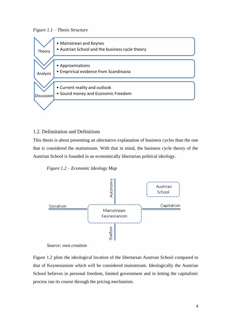
The structure of the thesis is outlined in figure 1.1.

4

Figure 1.1 – Thesis Structure

1.2. Delimitation and Definitions

This thesis is about presenting an alternative explanation of business cycles than the one

that is considered the mainstream. With that in mind, the business cycle theory of the

Austrian School is founded in an economically libertarian political ideology.

Figure 1.2 – Economic Ideology Map

Source: own creation

Figure 1.2 plots the ideological location of the libertarian Austrian School compared to

that of Keynesianism which will be considered mainstream. Ideologically the Austrian

School believes in personal freedom, limited government and in letting the capitalistic

process run its course through the pricing mechanism.

Theory

• Mainstrean and Keynes

• Austrian School and the business cycle theory

Analysis

• Approximations

• Emprirical evidence from Scandinavia

Discussion

• Current reality and outlook

• Sound money and Economic Freedom

5

In comparison Keynesianism involves relatively more government intervention,

socialism and regulation. Even though it is challenging to separate macroeconomics and

politics, the current thesis is about fundamental macroeconomic analysis of business

cycles. Thus, the fundamentals of the different political ideologies will not be subject to

extensive analysis.

The empirical analysis of business cycle theory in Scandinavia will include countries

Denmark, Norway and Sweden with the economic data collected ranging from first

fiscal quarter of 1980 to fourth fiscal quarter of 2010. The starting point of this time

span is selected so it will coincide with the analysis from the article by Bismans &

Mougeot (2009)1 in an effort to ensure comparability and validity of the results.

The findings from the Scandinavian countries will add a regional analysis to the

knowledge created by the article for comparison, as well as increasing the pool of

analyzed countries from four to seven. To help promote a holistic understanding of

business cycle theory and its implications, the remaining part of the thesis will not be

placed under the same geographical and temporal constraints.

Correlation coefficients are used for illustrative purposes rather than to infer causality.

Correlation in numbers does not automatically mean causation in a cause and effect

relationship. Conclusions will be drawn from the econometric tests with correlation

coefficients being purely used for indicating relationships and descriptive measures.

1 The empirical analysis of Bismans & Mougeot (2009) contains economic data from first fiscal quarter

1980 to fourth fiscal quarter 2005 for countries France, Germany, Great Britain and USA.

6

1.3. Literature Review

The number of empirical analyses on Austrian business cycle theory is limited. The

problematic point to analyzing the theory is the non-empirical proposition of its

hypotheses. There is an impractical measurability in being able to test them and a lack

of available technical methods available. An absence of constant relations and a control

group doesn‟t make the case easier as data from macroeconomic events consists of

historical data which is non-repeatable.

This thesis will be a part of the same pool of empirical examinations of the theory as the

Bismans & Mougeot article. The article which the methodological framework of the

current analysis is built on – finds that the term spread and the investment to

consumption expenditure ratio has significant effects on aggregate economic activity by

analyzing quarterly data.

Others publications who analyses the theory in similar fashion are Keeler (2001) who

use quarterly data for analyzing eight business cycles in USA from 1950 to 1991 and

finds consistent results that cycles are caused by monetary shocks and generated by

relative price changes. Mulligan (2006) analyzes monthly data on the relationship

between the interest rate spread, and the roundabout structure of production. He finds

evidence of co-integration between real consumable output and the cumulative interest

rate term spread.

7

2. Mainstream and Keynes

Every second, someone, somewhere is trading. What one can produce, others want to

consume. To pay for this consumption one must give something which the counterpart

places a value on and throughout history an exchange or ‟bartering‟ of goods or services

has taken place to make this work. The value or the amount of the payment is settled

between buyer and seller in the marketplace and is considered the price that enables the

transaction to go through. The price which the buyer and seller can agree on becomes

the compromising factor that leaves both parties satisfied. Valuing how much grain a

farmer had to pay a blacksmith to shoe his horse was somewhat manageable, but as

soon as trade becomes a little more sophisticated, including more links between

producer and end user and alternatives to choose from, it is a totally different story.

Money is a byproduct invented out of necessity as mankind and human interaction

progressed and developed, and has three primary functions. Firstly, it is a medium of

exchange which has eliminated the inefficiencies of the barter system, by being

generally accepted as payment for goods and services. Since precious metals such as

gold, silver and bronze are both scarce, fungible and reliable it has throughout history

been regarded as the monetary ideal (Ferguson, 2008). Secondly, it is a practical store of

value which is portable. It can be transported through time and across distances to allow

economic transactions for goods and services to be conducted - independently of

geographical and temporal constraints. Thirdly, it is a unit of account which facilitates

valuation calculation and most importantly price comparison.

The intangible character of most money today – virtual money – is perhaps the best

evidence of its true nature. Credit or „credo‟ in Latin means „I believe‟. Money is a

matter of belief or faith, that a certain value of it, can buy the supply of tangible goods

or intangible services. Though, the value of money, even precious metals are not

absolute; it is only worth what someone else is willing to pay for it in some other

valuable asset. An increase in the supply or notation of money will therefore not make

society richer or create prosperity.

8

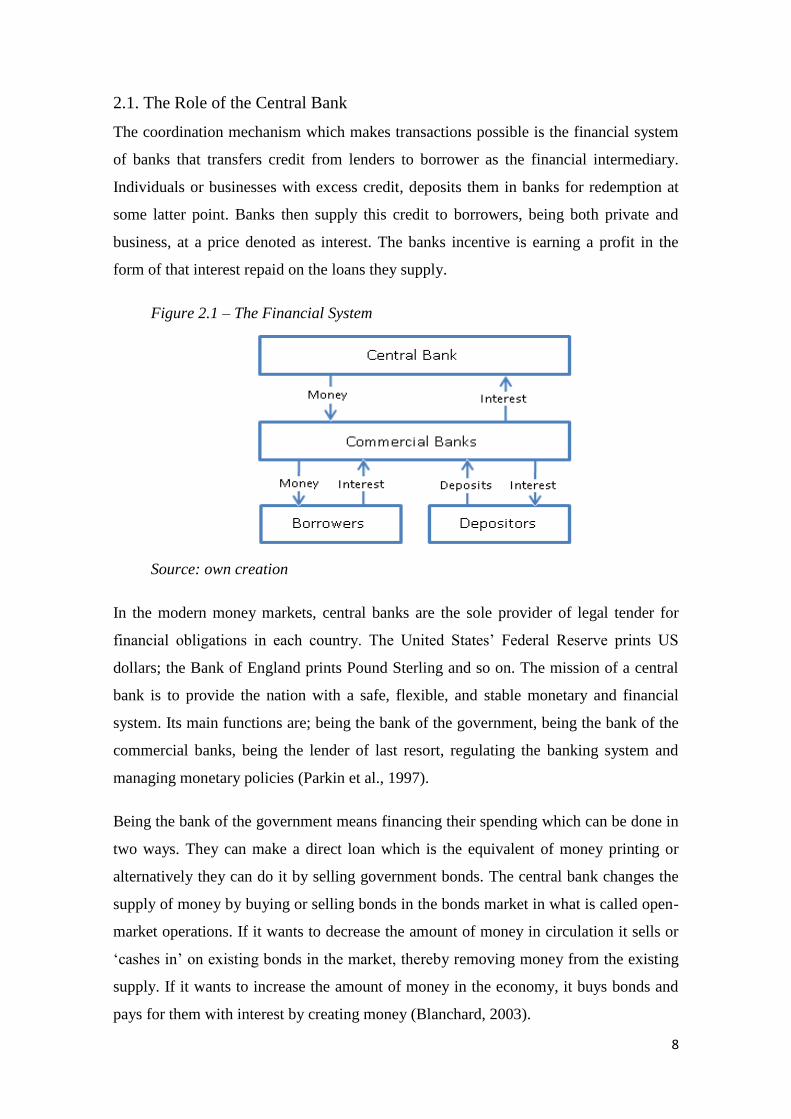
2.1. The Role of the Central Bank

The coordination mechanism which makes transactions possible is the financial system

of banks that transfers credit from lenders to borrower as the financial intermediary.

Individuals or businesses with excess credit, deposits them in banks for redemption at

some latter point. Banks then supply this credit to borrowers, being both private and

business, at a price denoted as interest. The banks incentive is earning a profit in the

form of that interest repaid on the loans they supply.

Figure 2.1 – The Financial System


In the modern money markets, central banks are the sole provider of legal tender for

financial obligations in each country. The United States‟ Federal Reserve prints US

dollars; the Bank of England prints Pound Sterling and so on. The mission of a central

bank is to provide the nation with a safe, flexible, and stable monetary and financial

system. Its main functions are; being the bank of the government, being the bank of the

commercial banks, being the lender of last resort, regulating the banking system and

managing monetary policies (Parkin et al., 1997).

Being the bank of the government means financing their spending which can be done in

two ways. They can make a direct loan which is the equivalent of money printing or

alternatively they can do it by selling government bonds. The central bank changes the

supply of money by buying or selling bonds in the bonds market in what is called open-

market operations. If it wants to decrease the amount of money in circulation it sells or

„cashes in‟ on existing bonds in the market, thereby removing money from the existing

supply. If it wants to increase the amount of money in the economy, it buys bonds and

pays for them with interest by creating money (Blanchard, 2003).

9

The price of these bonds and their interest rates has a natural relationship. The simplest

example is this; imagine a bond which promises to pay an amount of 100 at maturity in

one period e.g. in one year. If the price of that bond today is 90, the interest rate is given

by the following formula:

This yields an interest rate of 11.1%. If the price today is 80, the interest would be 25%.

This is a natural relationship because it eliminates any arbitrage opportunity. An amount

of 90 at 11.1% interest with one year to maturity gives 100. So, the lower the bond

price, the higher the interest rate and vice versa. Thus financing debt via open market

operations can be used to control the interest rate in the financial markets.

Being the bank of the commercial banks means keeping their reserves, regulating the

banking sector as well as being the lender of last resort. Keeping reserves is pretty

straight forward. Being the lender of last resort means extending credit to commercial

banks in the case of a credit crunch. By restoring the cash levels of commercial banks

helps to avoid a possible bank run. The interest rate at which the central bank is willing

to do this however have large implications.

Present day banking utilizes the law of large numbers since not all depositors arrive at

the same time to collect their money. This paves the way for fractional reserve banking

where banks by law are required only to retain a fraction of deposited capital for

immediate redemption. These regulations mean that the commercial banks can increase

the money supply with a multiplier, which is the amount of money that the initial

deposit can be expanded to. With a given minimum reserve ratio this multiplier is

calculated as the inverse of these reserve requirements:

Reserve requirements vary across countries and its balance sheet risk class but the target

of total capital a bank is required to hold is 8 % of its risk-weighted assets.2 This means

that the current money multiplier is 12.5.

2 Basel III – Minimum capital requirements. Basel III is a newly established global regulatory standard in

the stage of implementation and is targeted to be fully adopted by 2018 – bis.org

10

When commercial banks experience a one unit increase in deposits they are only

required to keep 8 % in reserves. The remaining 92 % can be loaned out to generate a

profit in received interest, resulting in a 12.5 unit increase compared to the initial

increase in deposits. The multiple expansions of loans and deposits allow them to create

a money supply which is larger with a multiple than the increase in the initial base. The

central bank can regulate the money supply by increasing the minimum requirements.

This would create a shortage of reserves and decrease lending which forces commercial

banks to increase the interest rate. The opposite is true for a lowering of the minimum

requirements.

The central bank can also directly set the interest rate at which commercial banks

borrow. Increasing the interest rate obviously makes it more expensive to loan from the

central bank encouraging commercial banks to cut their lending, whereas a fall in the

interest rate stimulates lending. Thus the central bank has great control over the money

supply and the interest rate at which commercial banks issue loans.

Like any other good, money and bonds are subject to supply and demand. When the

central bank adds to the pool of existing money, the supply is increased. The added

money eventually ends up as deposits in the commercial banks which in turn are loaned

out to maximize profits. When the commercial banks experience an increase in their

deposits they can lower the interest rate to attract borrowers and loan out the „excess‟

supply. The money supply is thereby increased with a multiple until the commercial

bank‟s balance sheets converge to match the minimum capital requirements.

The reason that central banks make changes in the money supply and change the interest

rate is a part of their mission to moderate business cycle fluctuations. Their tools for

doing this are the three presented in this section; open market operations, reserve

requirements and setting the discount rate towards commercial banks. Using these tools

is thereby a matter of objective to regulate aggregate economic activity and are

powerful macroeconomic instruments (Parkin et al., 1997).

11

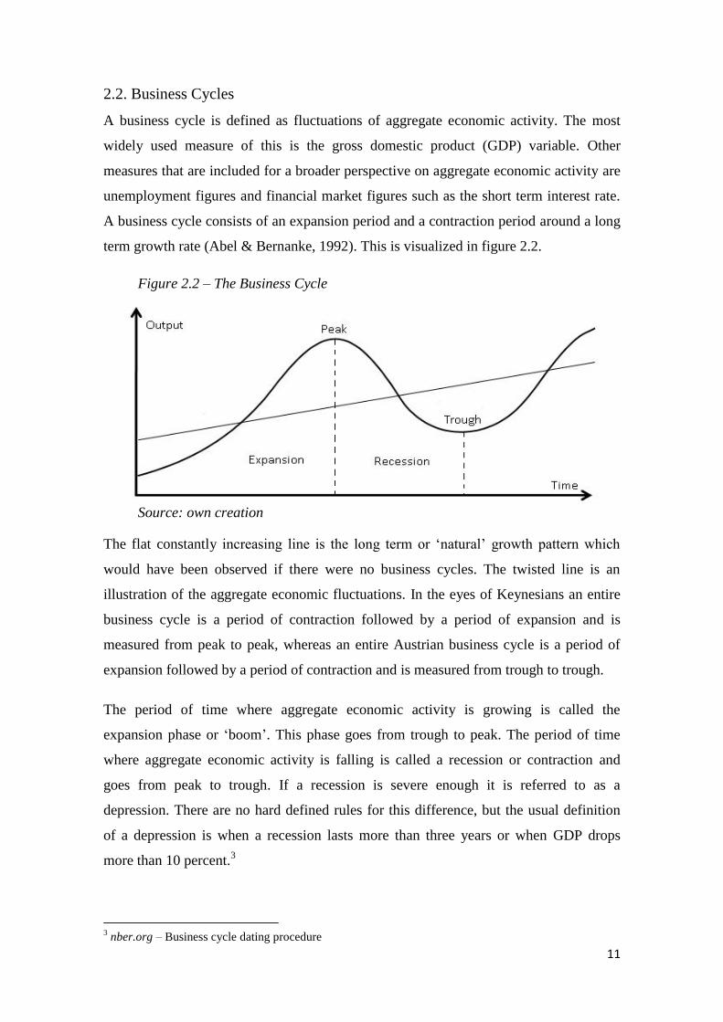
2.2. Business Cycles

A business cycle is defined as fluctuations of aggregate economic activity. The most

widely used measure of this is the gross domestic product (GDP) variable. Other

measures that are included for a broader perspective on aggregate economic activity are

unemployment figures and financial market figures such as the short term interest rate.

A business cycle consists of an expansion period and a contraction period around a long

term growth rate (Abel & Bernanke, 1992). This is visualized in figure 2.2.

Figure 2.2 – The Business Cycle


The flat constantly increasing line is the long term or „natural‟ growth pattern which

would have been observed if there were no business cycles. The twisted line is an

illustration of the aggregate economic fluctuations. In the eyes of Keynesians an entire

business cycle is a period of contraction followed by a period of expansion and is

measured from peak to peak, whereas an entire Austrian business cycle is a period of

expansion followed by a period of contraction and is measured from trough to trough.

The period of time where aggregate economic activity is growing is called the

expansion phase or „boom‟. This phase goes from trough to peak. The period of time

where aggregate economic activity is falling is called a recession or contraction and

goes from peak to trough. If a recession is severe enough it is referred to as a

depression. There are no hard defined rules for this difference, but the usual definition

of a depression is when a recession lasts more than three years or when GDP drops

more than 10 percent.3

3 nber.org – Business cycle dating procedure

12

These peaks and troughs are the turning points for the direction of aggregate economic

activity, and are of course of excessive interest to both media and policy makers alike.

Like stocks, businesses from different industries react differently to these changes in

GDP. Some may actually profit from a recession while others experience a greater deal

of financial distress than average.

Business cycles are hard to define but Korotayev & Tsirel (2010) identifies four

different types of business cycles. Ranging from the shortest to longest is; the Kitchin

cycle (1923) – averaging 40 months. This type of cycle concerns fluctuations in

inventories and the flow of information between decision makers and is generated by

market information asymmetries. This cycle is up for discussion with inventory

management and information flows being improved considerably through the

technological age. The Juglar cycle (1862) – identified as lasting 7-11 years, is an

investment cycle that observes investments into fixed capital and not just changes in

levels. The Kuznets swing (1930) – lasts 15 to 25 years, and is a wave of demographic

changes and infrastructural investments. Finally, the Kondratiev wave (1925) – lasting

50 to 60 years, captures fluctuations in wages, interest rates and raw material prices.

Business cycles are subject to extensive attention as they differ in timing, length, and

magnitude. This places a paramount uncertainty on the effects that a recession, or worse

a depression, has on the economy. The Keynesian approach to forecast and predict

cycles is to focus the attention on various indicative variables, with their direction and

timing being crucial for the planning of government intervention. Adopting this

inductive approach to analyzing business cycles means that it is important to understand

how these variable moves. Abel & Bernanke (1992) distinguish two important

characteristics that variables have in their behavior.

The first is the direction in movement relative to aggregate economic activity. An

economic variable which moves in the same direction as aggregate economic activity is

pro-cyclical. An economic variable which moves opposite to aggregate economic

activity is counter-cyclical and a variable which moves independently of aggregate

economic activity is a-cyclical.

Second, is the timing of the variables turning points relative to those of the business

cycle. If an economic variable‟s turning point is two to eight months before the turning

point of the business cycle it is considered a leading variable. If it is two months or

13

more after the turning point of aggregate economic activity, the variable is lagging and

if it is around the same time meaning +/- two months it is coincident.4

There is no doubt that the most interesting variables when forecasting are leading pro-

and counter-cyclical variables. OECD collects data on leading indicators which are

supposed to help analysts in their quest to forecast aggregate economic activity. Their

index of composite leading indicators for predicting business cycles consists of

variables which include the share price index, money supply and the interest rate

spread.5

Whereas Keynesians are busy looking for patterns in variables in order to explain and

predict cycles, Austrians explains cycles with the pattern of the money supply. The

hypothesis of the Austrian business cycle theory – and this thesis – that monetary

expansion causes business cycles raises a serious question about endogeneity in the

money supply variable. They argue that since the money supply is a leading variable

which is controlled solely by the central bank it must be explanatory of fluctuations in

aggregate economic activity.

When these cycles incur is uncertain. One thing which is known for sure is that no one

is able to exactly forecast the length, magnitude and turning points of these business

cycles. Keynesians are convinced that they have the necessary tools for avoiding a

recession when it emerges, whereas Austrians are convinced that they know what

causes the bubbles preceding a recession – and these two perceptions collide.

2.3. Keynesian Business Cycle Theory

Keynesianism stems from the work of British economist John Maynard Keynes (1883 –

1946) who was the author of the book; The General Theory of Employment, Interest and

Money published in 1936. At the time Keynes challenged the mainstream and

revolutionized economic thought. His work and principles, and in particular this

publishing, still to this day has a strong hold on mainstream macroeconomics. One of

Keynes‟ most notable contributions was the reversal of causality between supply and

demand.

4 OECD – System of composite leading indicators

5 Ibid.

14

French economist Jean-Baptiste Say (1767 – 1832) argued in his law of the market that;

“products are paid for with products” and that production of goods and services creates

incomes that are sufficient to buy those goods and services. This ultimately meant that

supply creates its own demand. Keynes challenged this argument and postulated that

aggregate economic activity does not depend on what can be produced – supply, but

instead on what people are willing to buy – demand (Parkin et al., 1997).

This means that by central economic planning via government intervention it is possible

to stimulate demand. By increasing demand, supply would have to increase as well to

meet this demand, offsetting an increase in production and employment creation. This

reasoning enables the government to assume a more active role in the pursuit of

reducing unemployment. Increasing demand is done by increasing the money supply.

Increasing the money supply means either directly giving people more money to spend

or encouraging consumption over saving with a lower rate of interest. The stimulus is

then meant to spur demand for goods, meaning companies must increase capacity and

hire more workers to produce goods.

Keynes also had his views on fluctuations in aggregate economic activity. According to

the Keynesian business cycle theory, fluctuations in aggregate economic activity are

influenced by changes in future expectations. Exogenous impulses are believed to alter

expectations about future sales and profits which in turn have an impact on demand for

capital and investments. Keynes reasoned that expectations are volatile because events

which shape the future are unknown and nearly impossible to forecast.

News and rumors about tax law alterations, interest rate changes, innovation and

political events, among many other factors, influence sales and profits. Assuming that

expectations are rational and because future sales and profits are nearly impossible to

forecast, there is reason to believe that it is rational to place expectations on rumors,

guesses, intuition and instinct. Also, it is rational to change one‟s expectations when

coming across new information.

Technically the impulses created by an altering of expectations are by Keynesian theory

what create business cycles. Changes in investments are made to accommodate these

changes in perception of the future. First, the changes in investments have a multiplier

effect as investments have an impact on aggregate expenditure, real GDP and

disposable income.

15

Changes in disposable income have an impact on consumption expenditure. Aggregate

demand then changes by a multiple of this initial change in investments. Second,

aggregate supply responds to a change in aggregate demand.

To fully understand why governments are given the authority to intervene in the

financial markets it is important to recognize the Keynesian assertion of decreases and

increases in aggregate demand. When aggregate demand decreases and unemployment

rises, the money wage6 does not change. Money wages are sticky in case of downward

adjustments. Reasons for this are minimum wage rules and labor market rigidity, along

with the (un)willingness to accept a lower pay. With a decrease in aggregate demand

and no change in the money wage rate the economy is stuck in unemployment

equilibrium.

No natural forces restore full employment. The economy will remain in this situation

until investments increase again. When aggregate demand increases and unemployment

falls, the money wage rate increases as there is not the same constraint on upwards

moving wages. With an increase in aggregate demand and an increase in money wages

the price level rise as well to eliminate shortages. The economy will remain in that

situation until investments and aggregate demand decrease (Parkin et al., 1997).

The main point in this story about increases and decreases in aggregate demand is that it

in both cases gets „stuck‟ until some outside force stimulates it. As explained earlier, the

government can do this by stimulating investments with alterations to the interest rate.

The reason the economy gets stuck is the removal of the money wage rates ability to

adjust itself downward when necessary. This is both brought on by minimum wage

regulation and people‟s willingness to accept – whichever comes first.

The prominent reason for the success of the Keynesian approach was its timing. The

Keynesian approach to business cycles came about in the 1930‟s during the great

depression at a time with high unemployment and economic turbulence. It seemed to

have all the answers for getting out of this situation compared to the invisible hand of

the free market which was deemed to be ineffective in doing so.

6 Money wage is the amount of money received in wages

16

The emergence of empirical testing of macroeconomic theories had made the „classic‟

or Austrian approach inconsistent with the data. Supported by empirical analysis

Keynes provided the tools for politicians to take action. He offered an explanation to

persistently high unemployment numbers founded in the assumption about sticky wages

and rigidity in the labor markets. The most illustrative contribution was how this

rigidity kept markets out of equilibrium, and how this could be solved with what

seemed a pain free solution. The government controlled improvement of

macroeconomic performance worked and it appeared that the main problems had been

solved.

It wasn‟t until the 1970‟s that the new approach came under pressure when the United

States suffered from both high unemployment and high inflation – a situation that

challenged the Keynesian approach as it was not coherent with the empirically proven

natural tradeoff between the two7 (Abel & Bernanke, 1992). Opposers to the Keynesian

approach were in no doubt as to why this happened. The Austrian School still to this

day argues that their „classical‟ approach contains the answers to the puzzling situation

in the 1970‟s and the origin of business cycles and growth altogether.

7 The inverse relationship between unemployment and inflation is expressed in the Phillips curve.

17

3. Austrian School of Economics

Austrian economists are mostly associated with political libertarianism due to their

belief in limited government and a laissez-faire approach to national economy. They

don‟t believe in government interfering in markets in which they are not agents and are

opposed to the Federal Reserve tinkering with money supply and interest rates.

Instead they believe that in order for an economy to prosper and create growth the

government should stop concentrating on what they can do, but instead on what not to

do. They counter the widespread mainstream economic argument that; failings of the

market need government intervention to be corrected, with the postulate that; no

government is able to echo the corrective mechanism of the market itself - the corrective

mechanism being the pricing system. Arguments for intervention in markets are brought

on by what is considered „market failings‟ in the form of free rider problems and

negative externalities, but according to Austrian theory, markets fail because of

government intervention and bureaucratic red tape.8

Advocates of the Austrian School of Economics and their way of thinking, differs from

mainstream economics in the sense that they base their conclusions on praxeology – the

study of human action. Ludwig von Mises – economist and social philosopher (1881-

1973) - proposed the axiom of action. The axiom, the proposition that humans act,

fulfills the requirements for a true synthetic a priori proposition (Hoppe, 1995). This

means that human action is deemed as an irrefutable fact in which individuals take

action towards their goals and that Austrian Schools‟ theories are thereby not derived

from numerical observations but rather founded on reflective understanding.

This distinction forms the basis for their main criticism of the mainstream economist‟s

use of mathematics and econometrics because economics, in their view, should be

understood and not observed. The pinnacle is then that followers of the Austrian School

believe that they preach a true understanding of economics. Their main headache is

though that in general opinion, empirical laws upon which Keynesian theory is built and

can be proven with numbers, offers the best truth.

8 mises.org – About the Mises Institute

18

Another important area of disagreement between the Austrian School and mainstream

economists – mainly Keynesian economists – is the concept of equilibrium. Keynes‟

equilibrium theory reflected his belief that national economy was a composition of

aggregate demand which, of course, is measurable, and that markets are in equilibrium

in the long run (Johnson et al, 2004). Mises on the other hand argues that markets, and

thereby prices, is a reflection of individual subjective value. In every market there is

voluntary exchange which can only be successful if there is cooperation or coordination.

Market problems thereby become coordination problems and not an expression of

aggregate measures (Herbener, 1991). The fact that Keynesian theories are based on the

condition of perfect equilibrium, or in other words, perfect coordination, must employ

some sort of systematic bias in the conclusions. Furthermore the Austrian School argues

that innovation and entrepreneurial profit seeking is what drives growth and, that

markets only have a tendency towards equilibrium (Kirzner, 1997).

3.1. Entrepreneurship

According to the Austrian School, entrepreneurship is central to creating the growth and

prosperity which Keynesian economists believe can be regulated by government

intervention. Entrepreneurs make new combinations of labor and natural resources with

the purpose of creating a profit. Entrepreneurs are concerned with future prices in

anticipating the direction of markets meaning that stabile prices are very much desired.

It is essential to be able to predict the lengths of time that will pass before the desired

change in prices have emerged, which also makes the timing determine whether projects

are successful or not. Entrepreneurs thus make a profit by providing future needs which

others have disregarded.9

Price changes in a market come from entrepreneurial arbitrage where an entrepreneur

buys commodities at the price they are willing to, puts them together and sells them

with a profit to someone who values this value enhancement. This makes production

and output through innovation and entrepreneurship the mainstay of Austrian economics

and the lifeblood of a healthy growing economy.

9 mises.org – The place of economics in learning: Forecasting as a profession

19

The entrepreneurial discovery approach views the market as an entrepreneurial driven

process. Mises stated that the driving force behind the market process is provided

neither by consumers or owners of land and capital goods but by profit seeking

entrepreneurship (Kirzner, 1997).

Consider an example with an isolated society consisting of three individuals. To

survive, each of them needs to catch and consume one fish per day by hand, a time

consuming task which provides just enough nutrition to make it to the next day. After a

period of time, one of them – the entrepreneur – gets an idea for a fishing net that will

make it easier to catch fish, leaving him with the option of catching more fish or having

more leisure time.

To make his idea come to life he must spend one day making this piece of capital

equipment, meaning that he will take on risk and underconsume. He will not have any

guarantee of whether he will succeed or not so he can be compensated for his sacrifice,

although if he does, he will initially be better off than the remaining two inhabitants.

Also, his demand for fish is unchanged but he chooses to forgo consumption that day to

potentially consume more in the future. Assuming that he succeeds with his invention

and puts the fishing net into productive use, he will be able to increase productivity

(catch more fish) and improve the living standards of not only himself but for all of this

small society.

With the help of this new piece of capital equipment the inhabitants are able to increase

production beyond the minimum amount which is needed to survive and are able to

consume more. The excess amount of fish caught – assuming that fish can be stored –

can be saved and/or used to feed the entrepreneur the day he decides to produce another

piece of capital equipment. Thus, an increase in productivity can generate savings which

in turn can be put to productive use and spur growth in an economy.

The inhabitants demand for fish was a driving factor behind the growth but in itself it is

not enough to achieve it. The key point is that the increase in productivity makes it

possible to consume more, and in the end, the economy doesn‟t grow because of an

increase in consumption. An increase in consumption is made possible because the

economy grows (Schiff, 2010).

20

This simple yet illustrative example shows the important role innovation and

entrepreneurship has in economic growth. To maximize the availability of scarce

resources is the very basics of economics and the more that can be produced, the more

can be consumed - tools, capital and innovation are the key to this. Being able to

produce (earn) more than the entrepreneur or business can consume means that the

excess goes into savings, which enables the economic benefits.

The personal gain from the profit seeking activity helps not only the entrepreneur

himself but raises the living standards of everyone. Because of the innovative

development all three inhabitants are able to catch and consume more fish – most

probably even leaving some to spare – either by copying the idea or borrowing the net.

Initially the entrepreneur gets relatively wealthier than the other two, but his profit

seeking activity – if successful - spills over on the rest of the society eventually. Had the

fishing net idea turned out to be a failure, his risk taking would not have been rewarded

and he would bear the losses himself without any immediate negative consequences for

the other two.

The innovative process created relative wealth and prosperity for the successful

entrepreneur. These degrees of wealth are, and have always been struck some as being

unfair. This agitation stems from a belief that the „rich‟ become rich because they take

wealth from others, whereas they actually create higher standards of living. This has

been labeled by Marxians as the „labor theory of value‟ where workers are underpaid

compared to what are worth. In their view the rich gets rich when they succeed in

making others poor. This has everything to do with moral posturing, and nothing to do

with reality (Schiff, 2010). What should instead be focused on is their ability to create

something of value which increases the standard of living for others; along with the jobs

they create to produce these things.

Prosperity and wealth is not created by printing money which can buy goods and spur

supply through demand. Instead, prosperity and wealth is achieved by raising living

standards. When entrepreneurs succeed it is because the goods or services which are

provided are valuable to others.

21

For Austrian economists it is important for self interest through profit seeking to be

allowed and promoted because it expands productive capacity and raises living

standards. Government regulation kills this entrepreneurial spirit by setting up

boundaries to enter the markets and progressive taxation decreases the incentive to

achieve.10

If however entrepreneurs do fail, the Austrian School is very clear about letting them

fail and be eliminated. Ideas and companies who are not able to survive are considered

to be a misallocation of capital. No matter the size of the companies and the loss of jobs,

those who have made wrongful decisions should be priced out of the market and the

capital which is left should be put to productive use. E.g. the productive equipment of a

bankrupt factory does not disappear from the surface of the earth. Other entrepreneurs

can buy the equipment and try to create a new company and create a profit when all the

black sheep have been eliminated. They may even need most of the former workers and

their skill and expertise.

When these companies are „bailed out‟ by government money, the unproductive and

unprofitable companies are kept alive which prevents the tied up capital from being put

to productive use. „Bailouts‟ actually promote an environment of bad decision making

by installing moral hazard in a „heads – I win, tails – everybody else loses‟ setting.

As described in this section, the importance of entrepreneurship has laid the foundation

for many of the ideologies of the Austrian School: the laissez-faire approach is

expressed in letting the pricing mechanism enable some to succeed and others to fail.

The libertarianism is expressed in letting those who succeed keep the fruits of their

labor while recognizing the improvement of living standards and jobs they create.

Furthermore it is important that the government interfere as little as possible to prevent

distortions in the market. Especially in the way the Keynesian approach where problems

in the economy are solved by inflationary monetary policies.

10

See Appendix A for the 2011 Heritage Foundation‟s assessment of the relationship between economic

freedom and innovation and entrepreneurship.

22

3.2. Inflation

According to the Austrian School, inflation is a result of an excess supply of money

compared to the demand for money11

. Inflation then exists when there is an increase in

the quantity of money. This will in turn raise the nominal price of any asset denoted in

that currency – in other words, it erodes the value of the currency compared to other

countries and causes a loss in purchasing power.

The money supply indicator is defined as pro-cyclical which means that it has its

turning point two to eight months prior to that of aggregate economic activity. Also, it is

a leading indicator meaning that when the money supply is increased, aggregate

economic activity increases afterwards (Abel & Bernanke, 1992). At a given amount of

money in the economy, the private banks would only be able to loan out that amount in

return of interest repaid with creation of real wealth. Under such a system the pricing of

loans would be the interest rate that the lender could repay in real wealth creation from

the generated profit. In the eyes of the Austrian School the scapegoat for inflation

creation is therefore the sole supplier of legal tender – the central bank.

The role of the central bank is to provide the means of exchange in the country, control

interest rates, supervise and regulate the banks and managing foreign exchange as an

independent entity. But, although a central bank is supposed to be independent, it is

their job to comply with the policies of the government in the financial markets. This

means financing deficit spending to avoid recessions and eliminate business cycles by

issuing loans or printing money. In that case, the supply of money must be increased

and hence inflation is created. When the central bank injects money into the fractional

reserve system, the private banks expand their level of credit. In this way the Austrian

School sees inflation as an increase in the money supply which causes prices to rise, and

not inflation as a result of rising prices (Schiff, 2009).

Ludwig von Mises elaborated on this definition. “Inflation means increasing the

quantity of money in circulation. But people use the term ‘inflation’ to refer to the

phenomenon that is an inevitable consequence of inflation, that is the tendency of all

prices and wage rates to rise. The result of this deplorable confusion is that there is no

term left to signify the cause of this rise in prices and wages. There is no longer any

11

Inflation can exist in any form of means of exchange. An increase in supply is simply an increase in the

number of units.

23

word available to signify the phenomenon that has been, up to now, called inflation…

As you cannot talk about something that has no name, you cannot fight it (Mises, 1951).

– “Inflation: An unworkable fiscal policy”

By this definition, expansionary monetary policies create inflation. Stabilizing prices are

both a priority for Keynesians and the Austrian School but the tools they employ are

very different. To avoid recessions in the Keynesian way the economy needs stimulus

which for Austrian economists are equivalent to inflation creation. In business planning

and entrepreneurial activity it is essential to be able to plan for the future because

companies are better off if they have some security that the value of their future

earnings will not suddenly fall or be subject to monetary policy distortions. The

Austrian School therefore places more importance on stabile prices compared to stabile

increasing prices.

There are few sound arguments for preventing prices to fall, but Keynesian theory has

created an almost universal acceptance that prices must rise in perpetuity. Austrians on

the other hand argue that prices actually fall naturally over time due to competition,

efficiency and technological progress - the most illustrative examples hereof being

technological goods. Computers, televisions and mobile phones have become both

better and cheaper since they were introduced, despite inflation. Also, when prices fall

and unemployment is high, people can afford to buy basic necessities. Keynesian

rigidity theory and labor market focus implies that falling prices are catastrophic

because companies‟ revenues decreases, but, in the Austrian „non-nominal notation of

value‟ approach, falling prices is actually the natural regulation mechanism (Schiff,

2009).

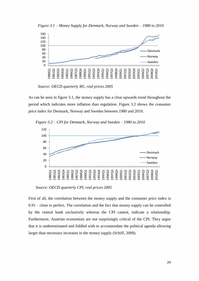
In order to assess the argument that an increase in the money supply causes prices to

rise, it is in its place to take a look at the development of the money supply and price

levels. The variables in question are money supply figures versus the consumer price

index, which is commonly used to measure inflation. The data upon which figure 3.3

and 3.4 are created, will be used for approximation for further analysis in the empirical

analysis in section 4.

24

Figure 3.1 – Money Supply for Denmark, Norway and Sweden – 1980 to 2010

Source: OECD quarterly M1, real prices 2005

As can be seen in figure 3.1, the money supply has a clear upwards trend throughout the

period which indicates more inflation than regulation. Figure 3.2 shows the consumer

price index for Denmark, Norway and Sweden between 1980 and 2010.

Figure 3.2 – CPI for Denmark, Norway and Sweden – 1980 to 2010

Source: OECD quarterly CPI, real prices 2005

First of all, the correlation between the money supply and the consumer price index is

0.91 – close to perfect. The correlation and the fact that money supply can be controlled

by the central bank exclusively whereas the CPI cannot, indicate a relationship.

Furthermore, Austrian economists are not surprisingly critical of the CPI. They argue

that it is underestimated and fiddled with to accommodate the political agenda allowing

larger than necessary increases in the money supply (Schiff, 2009).

020406080

100120140160

19

80

Q1

19

81

Q2

19

82

Q3

19

83

Q4

19

85

Q1

19

86

Q2

19

87

Q3

19

88

Q4

19

90

Q1

19

91

Q2

19

92

Q3

19

93

Q4

19

95

Q1

19

96

Q2

19

97

Q3

19

98

Q4

20

00

Q1

20

01

Q2

20

02

Q3

20

03

Q4

20

05

Q1

20

06

Q2

20

07

Q3

20

08

Q4

20

10

Q1

Denmark

Norway

Sweden

0

20

40

60

80

100

120

19

80

Q1

19

81

Q2

19

82

Q3

19

83

Q4

19

85

Q1

19

86

Q2

19

87

Q3

19

88

Q4

19

90

Q1

19

91

Q2

19

92

Q3

19

93

Q4

19

95

Q1

19

96

Q2

19

97

Q3

19

98

Q4

20

00

Q1

20

01

Q2

20

02

Q3

20

03

Q4

20

05

Q1

20

06

Q2

20

07

Q3

20

08

Q4

20

10

Q1

Denmark

Norway

Sweden

25

The shape of the two indices depicts the mechanisms of this. The concave nature of the

CPI development in figure 3.2 due to an allegedly constant adjustment of CPI figures

allows the convex nature of the money supply development in figure 3.1.

So far this section has presented the theoretical background of the Austrian School. The

alternative economic paradigm, the importance of entrepreneurship and the criticism of

the Keynesian inflationary policies are the key to fully understanding the reasoning

through the Austrian business cycle theory.

3.3. Austrian Business Cycle Theory

The Austrian business cycle theory was first introduced by Ludwig von Mises in 1912

in the book The Theory of Money and Credit and have since been developed and

complemented several times. The predominant contributors to this development are

Mises himself, Rothbard, Herberler and Hayek (Ebeling, 1978). The main criticism of

the Austrian business cycle theory is that its hypotheses are not founded in quantitative

observations. Instead the theory is developed through deductive logic reasoning which

lacks empirical evidence and therefore explanatory power (Bismans & Mougeot, 2009).

The theory though is very intuitive and has a high level of sophistication due to its

inclusion of unobservable variables. These - among others - include malinvestments and

malinvested capital and roundabout structure of production. But, this immeasurability of

variables creates the theory‟s own drawback since it, in the field of empirical analysis is

nearly impossible to include them. The theory propagates hypotheses about the

macroeconomic behavior subsequent to a monetary shock. According to the Austrian

School, monetary expansion to finance government spending sows the seed for a

business cycle to take place. The Austrian business cycle is no different than other

business cycles in its structure - the chronology of expansion, peak, recession and

trough is the same but its causal relationship is very different.

Keynesian business cycle theory states that it is the speculative expectation dynamics

which generates cycles by affecting marginal efficiency of investments and

subsequently the multiplier and output (Keynes, 1936), and that government should act

as an active savior by stimulating the economy out of a recessions.

26

Contrary to this, advocates of the Austrian School argue that the problem originates

with the distortive effects in the financial markets that these stimuli create (Schiff,

2010). Government spending and/or intervention are therefore considered the problem

and not the cure.

Injecting credit to the existing money supply creates inflation and lowers the interest

rate. This results in an expansion or „boom‟ where the economy experiences growth

rates which are higher than long term growth. Supply and demand theory says that when

supply is increased the value of a good is decreased. In this case the good is the

currency and the value of it is its depreciating relation towards foreign currencies. In

accordance with Keynesian theory, Mundell and Fleming (1962) argues that fiscal

spending actually makes the currency appreciate in the long run, but this has since been

subject to further empirical research. Penati (1985) and Obstfeld (2001) have countered

the argument in agreement with the Austrian School.

Increasing the money supply sends false signals to the capital market that there have

been an increase in savings and the interest rate is artificially depressed. When the

interest rate is lowered this way it no longer matches the natural time preference

between buyer and seller of credit. A monetary shock creates the difference between the

market rate and the natural rate, and represents the impulse that generates the business

cycle (Keeler, 2001). In the market for capital, lender and borrower responds to these

price alterations between the bank rate and the real rate of interest. This provides the

basis for a misallocation of capital and creates malinvestments.

3.3.1. Malinvestments

The concept of malinvestments is still subject of limited attention in mainstream

economics. For the Austrian School it is an important part of their argumentation for

their laissez-faire approach to national economy, which states that idle capital should

always be put into best possible productive use. If this allocation fails due to some

exogenous distortion instead of letting the market forces decide, capital is malinvested.

Consider a pool of idle savings ready to be invested. One possible use is profit-seeking

through entrepreneurial arbitrage by undertaking an investment project. To maximize

the return on an investment, one must consider the opportunity cost of doing so, facing

the choice between investing or receiving interest by lending the savings out to someone

27

else at the given market rate. When the market rate is artificially depressed, induced by

politics, more investment projects are undertaken.

This causal effect can be explained by the Net Present Value (NPV) relationship of

capital budgeting. The NPV rule states that projects should be undertaken when the

present value of future ingoing cash flows, minus the initial investment plus any future

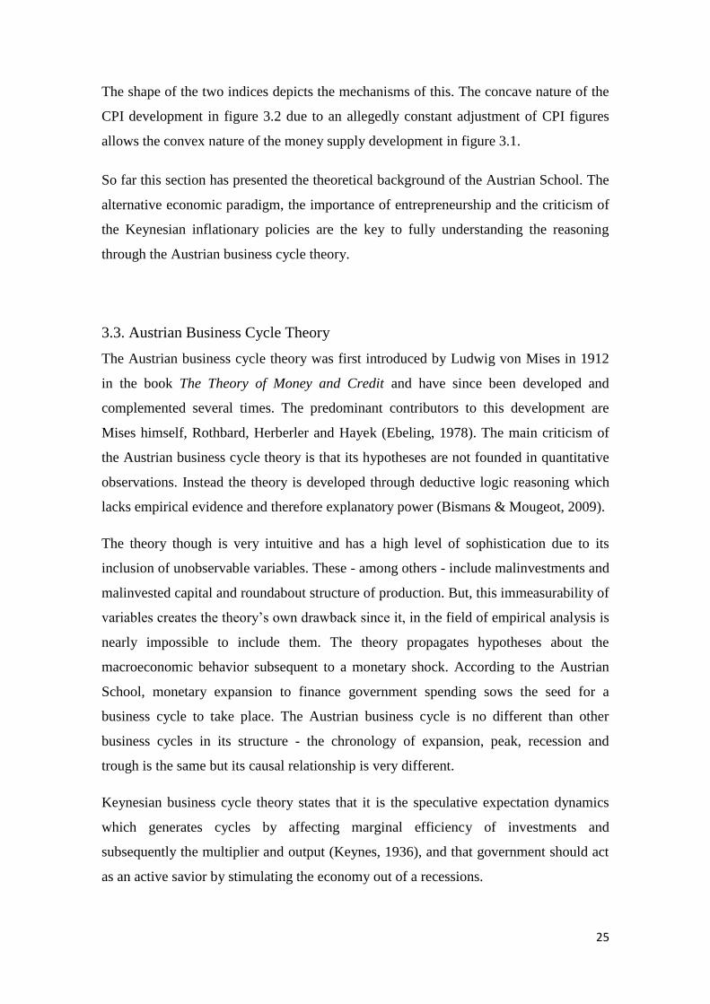
outgoing cash flows is positive. The relationship is depicted in figure 3.3.

Figure 3.3 – NPV Profile


The figure shows that when the discount rate – the cost of capital – is lowered, the NPV

of investment projects becomes more and more profitable. Thus, if the interest rate is

depressed, entrepreneurial activity gets more attractive compared to receiving interest,

and vice versa. Central planning of the interest rate as an instrument for financing policy

induced spending creates this distortive effect in the interest and investment market.

When politicians depress the interest rate by expansionary policies, projects that seemed

unprofitable become profitable.

Undertaking a malinvestment is analogue to buying a house with an adjustable

mortgage rate. If there is not room in the household budget for a future increase in the

interest rate, payments on the loan cannot be met. Should that happen and the house

should not have been bought in the first place.

Not only are these malinvestments created, the investments will go into earlier stages of

production which will result in a lengthening of the production process. The argument is

that producer prices rise compared to consumer prices in the expansionary phase

28

making it more attractive to invest in earlier stages. The production structure becomes

more roundabout as a result (Bismans & Mougeot, 2009).

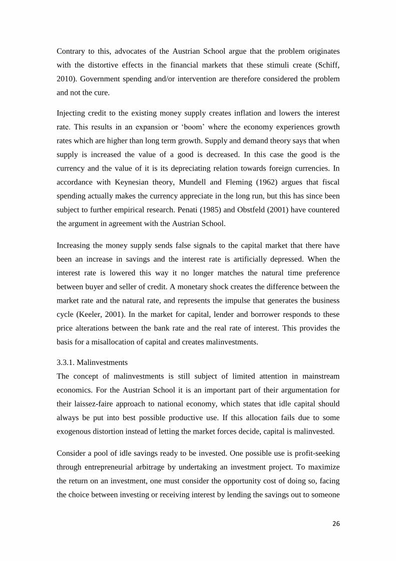
3.3.2. Roundabout Structure of Production

What happens when the interest rate is lowered by monetary expansion is that resources

shift away from later to earlier stages of production and becomes more roundabout

(Mulligan, 2006). Roundabout structure of production is the process of producing more

capital goods for the purpose of producing consumer goods. The roundabout process

begins with original input of resources – land and labor – to create a capital good to

assist the entrepreneur in achieving his goal. E.g. making a fishing net for catching fish

is a valuable capital good for the purpose but it does not directly catch the fish. The

process can be shown as an extension of the base line in the Hayekian triangle.

Figure 3.4 – Hayekian Triangle

Source: (Garrison, 2001)

When the base line is extended and/or the diagonal is flatter, it takes longer for final

output to consumers to be produced, and the process becomes more roundabout. With

an artificially depressed interest rate, firms invest more heavily in physical capital and

in the production process, and in projects with longer duration and lower expected

returns (Garrison, 2001).

Thus, cheaper financing makes it possible for this process to be more drawn out, and it

takes longer to produce the same amount of output delivered to consumers. As this shift

in demand by capital type towards more capital intensive processes takes place, a rise in

29

demand for capital for use in these early stages pushed their prices up, compared to

investments in stages closer to the consumer.

Along with malinvestments and a more roundabout production structure, a lowering of

the interest rate means that it becomes less preferable to save compared to consuming.

Consumers must be compensated for their patience for postponing consumption but

when this is reduced consumers spending will increase. Impatience and a lengthening of

the production structure do not go hand in hand and creates an unsustainable economy.

This unsustainable mismatch in supply and demand, where there is an excess demand

for consumer goods compared to the inadequate supply due to the more roundabout

production structure, means that consumer prices will eventually increase. It is

unsustainable because the depressed interest rate does not reflect another supply and

demand mechanism, namely household savings. The interest rate no longer reflects

agents lowered time preference as a function of a rise in household savings, but reflects

the derived effect of a monetary shock. In comparison, had the reduction in the interest

rate originated from an increase in household savings and less consumption, the agents

time preference would be reflected herein and be in line with the „roundaboutness‟ of

production. This argument is consistent with the Austrian Schools laissez-faire approach

to national economy, because without the artificial credit injection, the only pool of

funds available for investments would be household savings. Under such a regime, the

components concerning production structure and the cost of capital would more closely

match each other and reduce misallocation of capital.

The shortage of consumer goods and the following increase in consumer prices makes

investments in the later part of the process more preferable. This marks the Austrian

business cycles second shift in the production structure with a reversing of resource

allocation. Investments in the now more preferable later stages, increases demand for

capital and as a consequence of the putty-clay nature of capital12

, interest rates will rise

as the money supply is fixed without monetary authority intervention.

12

The Putty-Clay Model for capital investments (Gilchrist & Williams, 2000) is the recognition that

capital is liquid and can be moved freely (Putty), but once it is invested it becomes irreversible (Clay).

This means that investment in capital equipment displays an asymmetric reaction to large economic

shocks.

30

3.3.3. Liquidation and Summary

A rise in the interest rate means that economic growth will slow down and stagnate, or

maybe even decline as a result. This is by Keynesians considered more problematic than

by Austrians. Keynesian theory is concerned about the stickiness and rigidity of wages

and prices arguing that the market forces react too slow. Contrary to letting the markets

function under the pricing mechanism, Keynes believed that government spending and

monetary injection into the economy could spur an increase in demand for firms‟ goods

and keep people employed. This way, government intervention would help avoiding or

bringing the economy out of a recession (Abel & Bernanke, 1992).

The Austrian School on the other hand argues that a recession is necessary in order to

correct the malinvestments made during the boom preceding the bust. The key point

here is that Keynesians wants to prevent the bust of malinvestments whereas Austrians

wants to prevent the booms, created by false signals in the markets (Schiff, 2010).

Nevertheless, in an attempt to avoid a recession, or even worse a depression, the

monetary authorities will try to kick start the economy by increasing the money supply

even faster. They do this to try to maintain labor employment by keeping unhealthy

businesses afloat, but this will only prolong and enlarge the negative consequences of

their credit injection. As a consequence, the corrections in the market are much larger in

magnitude because liquidation of malinvestments have been prevented and kept alive by

stimuli. An argument for this type of policy is that the socioeconomic costs of a

recession are too large and intervention at some point becomes a necessity instead of an

option.

Furthermore, Keynesians argues that price stability is important and that deflation is

bad. What they don‟t seem to realize is that falling prices is part of the self-regulating

mechanism when unemployment lures. Austrians argue that they should instead let the

unprofitable companies fail and go out of business. This would open up the possibility

for entrepreneurs with access to excess capital, to buy up the valuable assets for profit

seeking activities - a process which would create new sustainable businesses and jobs.

31

To avoid an increase in the interest rate, the monetary authorities can keep injecting

money. Demand will though eventually outrun supply and interest rates will rise.

Projects and investments which were previously profitable are now abandoned and

liquidation of malinvestments begins. This liquidation phase signals the end of the

Austrian business cycle which can be summarized as follows:

1. The cycle is initiated when the central bank injects credit into the current money

supply to finance government spending. This creates a monetary shock, which causes

the market interest rate to fall below its natural level, creating an environment where

the depressed interest rate no longer matches the natural time preference.

2. An artificially depressed interest rate has two unhealthy implications; lower interest

means less household savings and more consumption. Also, it creates

malinvestments since more investment projects become profitable. Firms and

entrepreneurs now undertake more long term investments in capital goods.

3. These investments in earlier stages of production compared to investments in later

stages, implies that capital goods prices rise relative to consumer goods prices. The

production structure shift and become more roundabout.

4. With a longer and more roundabout production structure along with a lower

incentive to save, there will eventually be a shortage of consumer goods. This will in

turn drive consumer prices up and make investments in later stages of production

more preferable compared to investments in earlier stages.

5. Reversing the resource allocation creates an increase in demand for credit. This

increase in demand is absorbed by a rising interest rate. To avoid rising interest rates

leading to a recession and a loss of jobs, the monetary authorities can again increase

the money supply in an attempt to get the economy going again.

6. Even though the central bank in principle could keep printing and injecting money,

demand eventually outruns supply and the interest rate rises again. Projects and

investments are abandoned and liquidation of malinvestments begins.

32

The central bank could in principle keep injecting money into the economy if they

believe that the tide will eventually turn by going deeper into debt, but this would have

implications of the currency and is rather unsustainable.13

The role of price signals is essential throughout the cycle‟s line of reasoning. Every

development is a reaction to pricing signals in any of the events. First, the decreased

price of capital creates malinvestments. Second, investments in earlier stages are

undertaken because relative price of production to consumer goods is distorted. Third, a

shortage of consumer goods will drive prices up and make later stage investments

profitable and finally, again the increase in the price of capital offsets malinvestment

liquidation and the recession.

This section has outlined important principles in the paradigm of the Austrian School

with respect to the Austrian business cycle explanation. In the pursuit „proof‟ in the eyes

of mainstream Keynesians, the theory will in the following section will be subject to

empirical analysis.

13

mises.org – The coming currency crisis and the Downfall of the Dollar

33

4. Evidence from Scandinavia

The purpose of the chosen approach in this analysis is to explain and conclude on the

conceptual theoretical business cycle theory as presented by the Austrian School, using

the analytical tools employed by mainstream analysts. In other words, explaining logical

deduction with empirical econometrics. In order to use econometric tools to analyze the

hypotheses of the Austrian business cycle theory, it is necessary to make a number of

approximations since the pure presentation of the cycle is non-empirical. To test these

hypotheses the conceptual theoretical framework must be converted into statistical

numeric terms which is done in this section. The analysis will be based on the

methodological framework of Bisman & Mougeot (2009).

The countries which are subject to this analysis are the three Scandinavian countries;

Denmark, Norway and Sweden. Others than being defined under the region of

Scandinavia, these three countries share some features. They all share the government

form of a unified parliamentary democracy under a constitutional monarchy. They all

have their own currencies – the Krone – with Norway and Sweden‟s being a floating

currency and Denmark‟s being a pegged exchange rate with a horizontal band. This

implies that they are all managing their own monetary policies, but Denmark‟s is

limited against the Euro by +/- 2.25%.

A note on Norway is that they are the world‟s largest producer of oil and natural gasses

per capita outside the Middle-East.14

This is believed to be the main reason for the

discrepancy of the Norwegian ratio in figure 4.3 compared to Denmark and Sweden,

because more money is left to be saved after consumption.

Ranked by the Heritage Foundation‟s economic freedom index, Denmark is 78.7 out of

100, Norway is 71.9 and Sweden is 70.3 placed at 8th

, 22nd

and 30th

respectively.15

This

leaves all three countries in the „mostly free‟ category.

Analyzing these three countries using the methodology of Bismans & Mougeot will add

to the knowledge they created and increase the number of analyzed countries from four

to seven. Furthermore, it will provide a regional analysis of Scandinavia.

14

CIA – World Fact Book - Norway 15

heritage.org – Economic Freedom

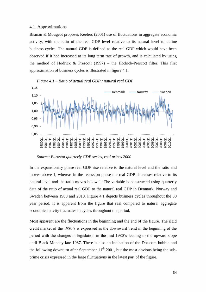
34

4.1. Approximations

Bisman & Mougeot proposes Keelers (2001) use of fluctuations in aggregate economic

activity, with the ratio of the real GDP level relative to its natural level to define

business cycles. The natural GDP is defined as the real GDP which would have been

observed if it had increased at its long term rate of growth, and is calculated by using

the method of Hodrick & Prescott (1997) – the Hodrick-Prescott filter. This first

approximation of business cycles is illustrated in figure 4.1.

Figure 4.1 – Ratio of actual real GDP / natural real GDP

Source: Eurostat quarterly GDP series, real prices 2000

In the expansionary phase real GDP rise relative to the natural level and the ratio and

moves above 1, whereas in the recession phase the real GDP decreases relative to its

natural level and the ratio moves below 1. The variable is constructed using quarterly

data of the ratio of actual real GDP to the natural real GDP in Denmark, Norway and

Sweden between 1980 and 2010. Figure 4.1 depicts business cycles throughout the 30

year period. It is apparent from the figure that real compared to natural aggregate

economic activity fluctuates in cycles throughout the period.

Most apparent are the fluctuations in the beginning and the end of the figure. The rigid

credit market of the 1980‟s is expressed as the downward trend in the beginning of the

period with the changes in legislation in the mid 1980‟s leading to the upward slope

until Black Monday late 1987. There is also an indication of the Dot-com bubble and

the following downturn after September 11th

2001, but the most obvious being the sub-

prime crisis expressed in the large fluctuations in the latest part of the figure.

0,85

0,90

0,95

1,00

1,05

1,10

1,15

19

80

Q1

19

81

Q1

19

82

Q1

19

83

Q1

19

84

Q1

19

85

Q1

19

86

Q1

19

87

Q1

19

88

Q1

19

89

Q1

19

90

Q1

19

91

Q1

19

92

Q1

19

93

Q1

19

94

Q1

19

95

Q1

19

96

Q1

19

97

Q1

19

98

Q1

19

99

Q1

20

00

Q1

20

01

Q1

20

02

Q1

20

03

Q1

20

04

Q1

20

05

Q1

20

06

Q1

20

07

Q1

20

08

Q1

20

09

Q1

20

10

Q1

Denmark Norway Sweden

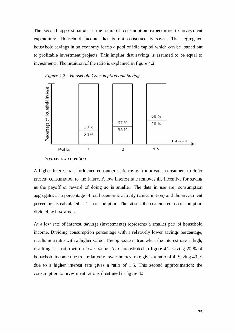
35

The second approximation is the ratio of consumption expenditure to investment

expenditure. Household income that is not consumed is saved. The aggregated

household savings in an economy forms a pool of idle capital which can be loaned out

to profitable investment projects. This implies that savings is assumed to be equal to

investments. The intuition of the ratio is explained in figure 4.2.

Figure 4.2 – Household Consumption and Saving


A higher interest rate influence consumer patience as it motivates consumers to defer

present consumption to the future. A low interest rate removes the incentive for saving

as the payoff or reward of doing so is smaller. The data in use are; consumption

aggregates as a percentage of total economic activity (consumption) and the investment

percentage is calculated as 1 – consumption. The ratio is then calculated as consumption

divided by investment.

At a low rate of interest, savings (investments) represents a smaller part of household

income. Dividing consumption percentage with a relatively lower savings percentage,

results in a ratio with a higher value. The opposite is true when the interest rate is high,

resulting in a ratio with a lower value. As demonstrated in figure 4.2, saving 20 % of

household income due to a relatively lower interest rate gives a ratio of 4. Saving 40 %

due to a higher interest rate gives a ratio of 1.5. This second approximation; the

consumption to investment ratio is illustrated in figure 4.3.

36

Figure 4.3 – Ratio of Consumption expenditure / Investment expenditure

Source: Eurostat – final consumption as a percentage of GDP, quarterly data

This ratio also captures the fluctuations in the changes of final goods production and

capital goods production, and is an indicator of the production structure distortion

through business cycles as proposed by the Hayekian Triangle. The ratio tends to

increase during the last part of expansion and tends to decrease at the end of recessions.

Figure 4.3 shows the investment pattern most clearly in the later part of the figure

compared to figure 4.1. The pattern of the variable characterizes the more roundabout

production process with a relative increase in capital goods production in the

expansionary phase followed by a rise in consumption goods production. The maxima

of the ratio are reached during the recession or during the quarters just after recessions,

supporting the Austrian hypothesis that malinvestment liquidation concludes the cycle

(Bismans & Mougeot, 2009).

The third approximation is expressed in the ratio of consumption price index to

production price index as an indication of relative prices through the cycle caused by

monetary shocks. The ratio is constructed using the consumer price index divided by the

producer price index. Relative prices are distorted by changes in the market interest rate

and when the interest rate is lowered, demand for capital goods increase and capital

goods prices goes up relative to final good prices (Keeler, 2001). This third

approximation of relative prices is illustrated in figure 4.4.

1,00

1,50

2,00

2,50

3,00

3,50

4,00

4,50

5,00

5,501

98

0Q

11

98

1Q

11

98

2Q

11

98

3Q

11

98

4Q

11

98

5Q

11

98

6Q

11

98

7Q

11

98

8Q

11

98

9Q

11

99

0Q

11

99

1Q

11

99

2Q

11

99

3Q

11

99

4Q

11

99

5Q

11

99

6Q

11

99

7Q

11

99

8Q

11

99

9Q

12

00

0Q

12

00

1Q

12

00

2Q

12

00

3Q

12

00

4Q

12

00

5Q

12

00

6Q

12

00

7Q

12

00

8Q

12

00

9Q

12

01

0Q

1

Denmark Norway Sweden

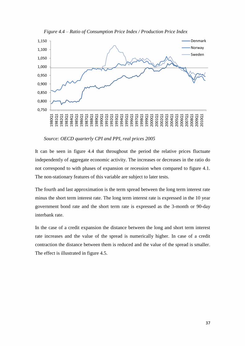
37

Figure 4.4 – Ratio of Consumption Price Index / Production Price Index

Source: OECD quarterly CPI and PPI, real prices 2005

It can be seen in figure 4.4 that throughout the period the relative prices fluctuate

independently of aggregate economic activity. The increases or decreases in the ratio do

not correspond to with phases of expansion or recession when compared to figure 4.1.

The non-stationary features of this variable are subject to later tests.

The fourth and last approximation is the term spread between the long term interest rate

minus the short term interest rate. The long term interest rate is expressed in the 10 year

government bond rate and the short term rate is expressed as the 3-month or 90-day

interbank rate.

In the case of a credit expansion the distance between the long and short term interest

rate increases and the value of the spread is numerically higher. In case of a credit

contraction the distance between them is reduced and the value of the spread is smaller.

The effect is illustrated in figure 4.5.

0,750

0,800

0,850

0,900

0,950

1,000

1,050

1,100

1,150

19

80

Q1

19

81

Q1

19

82

Q1

19

83

Q1

19

84

Q1

19

85

Q1

19

86

Q1

19

87

Q1

19

88

Q1

19

89

Q1

19

90

Q1

19

91

Q1

19

92

Q1

19

93

Q1

19

94

Q1

19

95

Q1

19

96

Q1

19

97

Q1

19

98

Q1

19

99

Q1

20

00

Q1

20

01

Q1

20

02

Q1

20

03

Q1

20

04

Q1

20

05

Q1

20

06

Q1

20

07

Q1

20

08

Q1

20

09

Q1

20

10

Q1

Denmark

Norway

Sweden

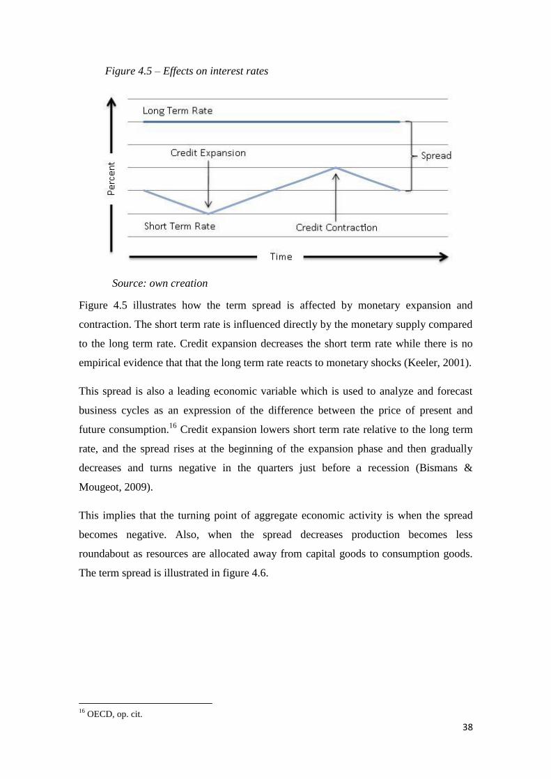
38

Figure 4.5 – Effects on interest rates


Figure 4.5 illustrates how the term spread is affected by monetary expansion and

contraction. The short term rate is influenced directly by the monetary supply compared

to the long term rate. Credit expansion decreases the short term rate while there is no

empirical evidence that that the long term rate reacts to monetary shocks (Keeler, 2001).

This spread is also a leading economic variable which is used to analyze and forecast

business cycles as an expression of the difference between the price of present and

future consumption.16

Credit expansion lowers short term rate relative to the long term

rate, and the spread rises at the beginning of the expansion phase and then gradually

decreases and turns negative in the quarters just before a recession (Bismans &

Mougeot, 2009).

This implies that the turning point of aggregate economic activity is when the spread

becomes negative. Also, when the spread decreases production becomes less

roundabout as resources are allocated away from capital goods to consumption goods.

The term spread is illustrated in figure 4.6.

16

OECD, op. cit.

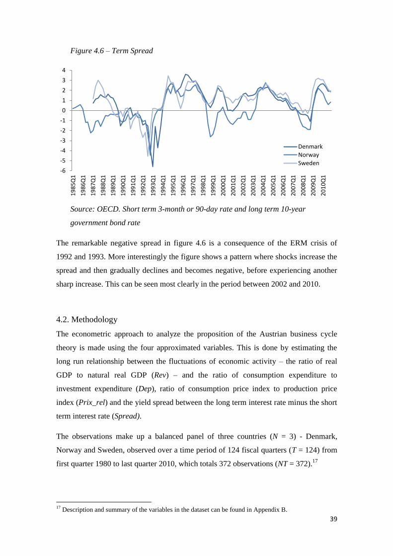
39

Figure 4.6 – Term Spread

Source: OECD. Short term 3-month or 90-day rate and long term 10-year

government bond rate

The remarkable negative spread in figure 4.6 is a consequence of the ERM crisis of

1992 and 1993. More interestingly the figure shows a pattern where shocks increase the

spread and then gradually declines and becomes negative, before experiencing another

sharp increase. This can be seen most clearly in the period between 2002 and 2010.

4.2. Methodology

The econometric approach to analyze the proposition of the Austrian business cycle

theory is made using the four approximated variables. This is done by estimating the

long run relationship between the fluctuations of economic activity – the ratio of real

GDP to natural real GDP (Rev) – and the ratio of consumption expenditure to

investment expenditure (Dep), ratio of consumption price index to production price

index (Prix_rel) and the yield spread between the long term interest rate minus the short

term interest rate (Spread).

The observations make up a balanced panel of three countries (N = 3) - Denmark,

Norway and Sweden, observed over a time period of 124 fiscal quarters (T = 124) from

first quarter 1980 to last quarter 2010, which totals 372 observations (NT = 372).17

17

Description and summary of the variables in the dataset can be found in Appendix B.

-6

-5

-4

-3

-2

-1

0

1

2

3

41

98

5Q

1

19

86

Q1

19

87

Q1

19

88

Q1

19

89

Q1

19

90

Q1

19

91

Q1

19

92

Q1

19

93

Q1

19

94

Q1

19

95

Q1

19

96

Q1

19

97

Q1

19

98

Q1

19

99

Q1

20

00

Q1

20

01

Q1

20

02

Q1

20

03

Q1

20

04

Q1

20

05

Q1

20

06

Q1

20

07

Q1

20

08

Q1

20

09

Q1

20

10

Q1

Denmark

Norway

Sweden

40

The baseline model for this panel dataset is:

where yit is the dependent variable, β0 the constant, xit the independent variables, β the

coefficients for each independent variable, αi is the unknown country specific intercept

and uit the error term. The long run relationship is estimated, in this paper, with a fixed

effects model and by fitting the variables into equation 1 the following model is

obtained:

where αi is the deterministic constant specific to each of the three countries. When using

fixed effects it is assumed that there is something within each country that may impact

or bias the outcome which must be controlled for. This is done by estimating country

specific intercepts.

4.3. Empirical Evidence

In the pursuit of statistical inference in this empirical analysis, stationarity of the

variables needs to be tested. In order to stay clear of spurious regression problems the

variables must be stationary, which is done by unit root tests.

4.3.1. Unit root test

As panel data consists of time series, the assumptions for time series analysis, analogue

to the classical Gauss-Markov assumptions, must be fulfilled (Wooldridge, 2006).

Stationarity is a basic requirement for time series modeling which implies that the mean,

variance and autocorrelation structure of the variables are independent of time. The unit

root tests for stationary variables are performed with the use of the Augmented Dickey-

Fuller test and the Phillips-Perron test, with lags included to control for higher-order

autoregressive components.

The tests combine the p-values from the separate unit root test on each panel to obtain

an overall test of whether the panel series contains a unit root.18

18

Stata output for Dickey-Fuller and Phillips-Perron tests of all variables can be found in Appendix C.

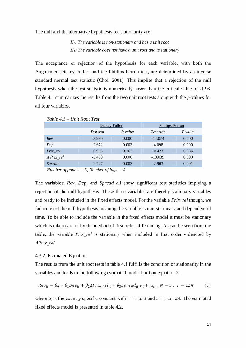
41

The null and the alternative hypothesis for stationarity are:

H0: The variable is non-stationary and has a unit root

H1: The variable does not have a unit root and is stationary

The acceptance or rejection of the hypothesis for each variable, with both the

Augmented Dickey-Fuller -and the Phillips-Perron test, are determined by an inverse

standard normal test statistic (Choi, 2001). This implies that a rejection of the null

hypothesis when the test statistic is numerically larger than the critical value of -1.96.

Table 4.1 summarizes the results from the two unit root tests along with the p-values for

all four variables.

Table 4.1 – Unit Root Test

Dickey Fuller Phillips-Perron

Test stat P value Test stat P value

Rev -3.990 0.000 -14.074 0.000

Dep -2.672 0.003 -4.098 0.000

Prix_rel -0.965 0.167 -0.423 0.336

Δ Prix_rel -5.450 0.000 -10.039 0.000

Spread -2.747 0.003 -2.903 0.001

Number of panels = 3, Number of lags = 4

The variables; Rev, Dep, and Spread all show significant test statistics implying a

rejection of the null hypothesis. These three variables are thereby stationary variables

and ready to be included in the fixed effects model. For the variable Prix_rel though, we

fail to reject the null hypothesis meaning the variable is non-stationary and dependent of

time. To be able to include the variable in the fixed effects model it must be stationary

which is taken care of by the method of first order differencing. As can be seen from the

table, the variable Prix_rel is stationary when included in first order - denoted by

ΔPrix_rel.

4.3.2. Estimated Equation

The results from the unit root tests in table 4.1 fulfills the condition of stationarity in the

variables and leads to the following estimated model built on equation 2:

where αi is the country specific constant with i = 1 to 3 and t = 1 to 124. The estimated

fixed effects model is presented in table 4.2.

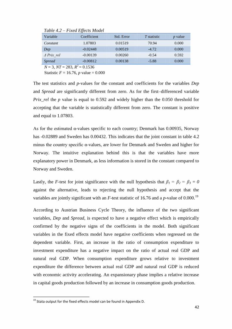
42

Table 4.2 – Fixed Effects Model

Variable Coefficient Std. Error T statistic p value

Constant 1.07803 0.01519 70.94 0.000

Dep -0.02448 0.00519 -4.72 0.000

Δ Prix_rel -0.00139 0.00260 -0.54 0.592

Spread -0.00812 0.00138 -5.88 0.000

N = 3, NT = 283, R2 = 0.1536

Statistic F = 16.76, p value = 0.000

The test statistics and p-values for the constant and coefficients for the variables Dep

and Spread are significantly different from zero. As for the first–differenced variable

Prix_rel the p value is equal to 0.592 and widely higher than the 0.050 threshold for

accepting that the variable is statistically different from zero. The constant is positive

and equal to 1.07803.

As for the estimated α-values specific to each country; Denmark has 0.00935, Norway

has -0.02889 and Sweden has 0.00432. This indicates that the joint constant in table 4.2

minus the country specific α-values, are lower for Denmark and Sweden and higher for

Norway. The intuitive explanation behind this is that the variables have more

explanatory power in Denmark, as less information is stored in the constant compared to

Norway and Sweden.

Lastly, the F-test for joint significance with the null hypothesis that β1 = β2 = β3 = 0

against the alternative, leads to rejecting the null hypothesis and accept that the

variables are jointly significant with an F-test statistic of 16.76 and a p-value of 0.000.19

According to Austrian Business Cycle Theory, the influence of the two significant

variables, Dep and Spread, is expected to have a negative effect which is empirically

confirmed by the negative signs of the coefficients in the model. Both significant

variables in the fixed effects model have negative coefficients when regressed on the

dependent variable. First, an increase in the ratio of consumption expenditure to

investment expenditure has a negative impact on the ratio of actual real GDP and

natural real GDP. When consumption expenditure grows relative to investment

expenditure the difference between actual real GDP and natural real GDP is reduced

with economic activity accelerating. An expansionary phase implies a relative increase

in capital goods production followed by an increase in consumption goods production.

19

Stata output for the fixed effects model can be found in Appendix D.

43

When the cycle turns into a recession natural GDP then outgrows actual GDP resulting

in liquidation of malinvestments. Second, an increase in the term spread also means a

decrease in the ratio of actual real GDP to natural real GDP. Monetary expansion lowers

the short term interest rate which widens the gap between the long term rate and the

short term rate. When the term spread increases it brings real economic activity to

accelerate compared to its natural GDP until the short term market interest rate

converges to its natural level.

4.3.3. Post-estimation

Post-estimation verifies the fixed effects model and the results can be seen in appendix

E. The Hausman test for testing the fixed effects model against a random effects model

shows a strong significance in favor of the fixed version. Serial correlation test shows

that there is no serial correlation in the residuals with the test unsuccessful in rejecting

the null hypothesis for just that. Wald tests for testing the linear relationship of the

explanatory variables yields significant results for the consumption to investment ratio

and the term spread but not for the relative price ratio as expected. Finally, testing for

the country specific effects, results in a rejection of the null hypothesis that these are

jointly significant.20

20

Stata output for post-estimation of the fixed effects model can be found in Appendix E.

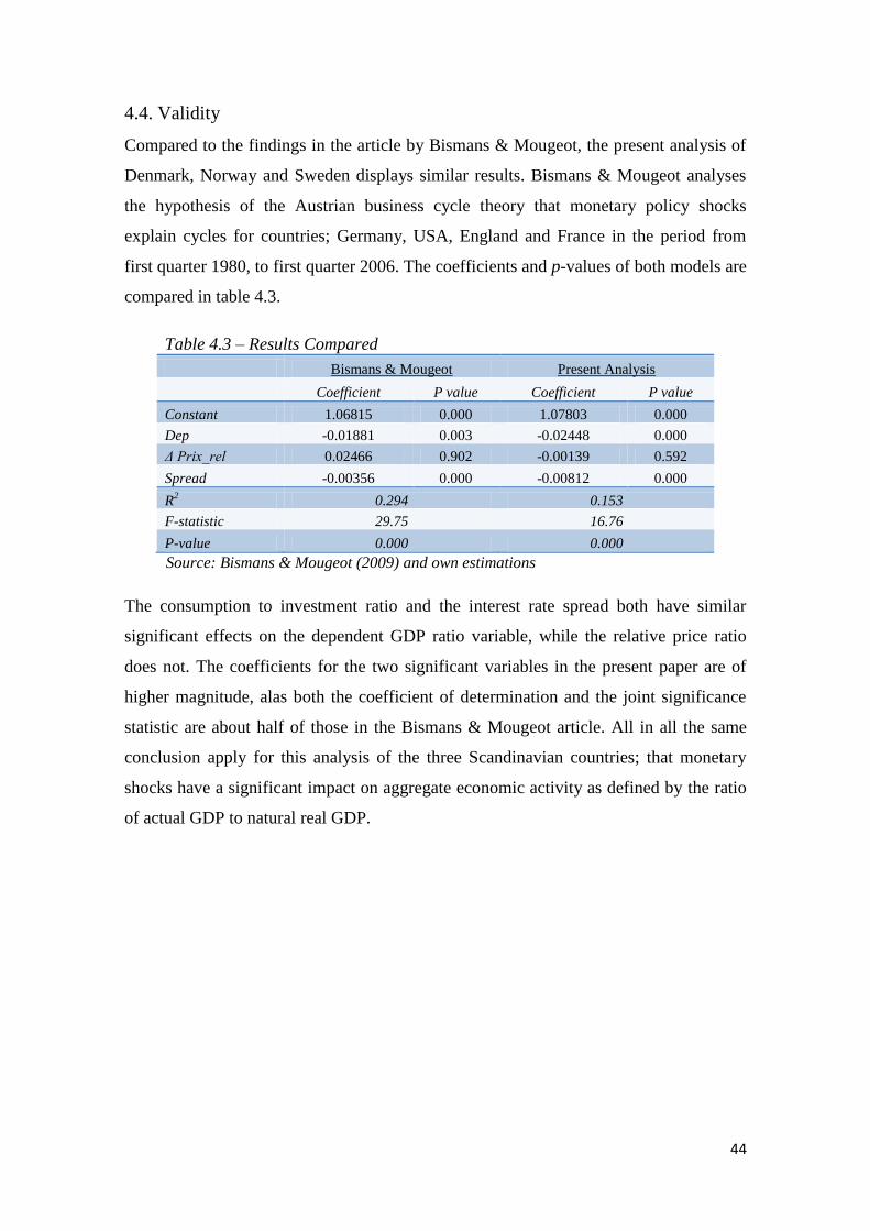
44

4.4. Validity

Compared to the findings in the article by Bismans & Mougeot, the present analysis of

Denmark, Norway and Sweden displays similar results. Bismans & Mougeot analyses

the hypothesis of the Austrian business cycle theory that monetary policy shocks

explain cycles for countries; Germany, USA, England and France in the period from

first quarter 1980, to first quarter 2006. The coefficients and p-values of both models are

compared in table 4.3.

Table 4.3 – Results Compared

Bismans & Mougeot Present Analysis

Coefficient P value Coefficient P value

Constant 1.06815 0.000 1.07803 0.000

Dep -0.01881 0.003 -0.02448 0.000

Δ Prix_rel 0.02466 0.902 -0.00139 0.592

Spread -0.00356 0.000 -0.00812 0.000

R2 0.294 0.153

F-statistic 29.75 16.76

P-value 0.000 0.000

Source: Bismans & Mougeot (2009) and own estimations

The consumption to investment ratio and the interest rate spread both have similar

significant effects on the dependent GDP ratio variable, while the relative price ratio

does not. The coefficients for the two significant variables in the present paper are of

higher magnitude, alas both the coefficient of determination and the joint significance

statistic are about half of those in the Bismans & Mougeot article. All in all the same

conclusion apply for this analysis of the three Scandinavian countries; that monetary

shocks have a significant impact on aggregate economic activity as defined by the ratio

of actual GDP to natural real GDP.

45

5. Discussion

The results from the empirical analysis support those of Bismans & Mougeot. The

results apply not only in Scandinavia but also for more dominant economies such as the

United States, Britain, France and Germany, concluding that monetary policy shocks

explain business cycles.

Going deeper into debt when debt is already serious is a puzzling argument, but that is

the reality of the world‟s largest economy as of 2011.21

The argument of doing so builds

on theories proposed by Keynes which says that a government spending is necessary in

order to prosper and avoid recessions. Intuitively it is backwards thinking that

prosperity and spending comes before a period of saving which enables you to pay for

it. Many private household would share this intuition. Keynes though argued that in

order to get the economic wheels going a credit injection into the economy is needed.

The timing of Keynes work could not have been better though. After more than a

century of prosperity and growth of productive capacity and rising living standards, the

western world with the United States in front could afford the luxury of the economic

policies of Keynes. In the middle of the 20th

century, the United States was the world‟s

leading creditor nation with more money loaned out to others than all other creditor

nations put together. Today the United States are exactly the opposite, being the largest

debtor nation with more debt to the rest of the world than all debtor nations put together

(Schiff, 2009). The prosperity which had been created, especially in the United States,

was driven by free enterprise, individual property rights and limited government which

the founding fathers of the Unites States of America ensured in their constitution.

Keynesian theories remained dominant in the post-war period and after decades of pain

free solutions to unemployment problems and recessions by political intervention, many

policymakers viewed the non-interventionist approach to business cycles as being

politically unacceptable. In the 1960‟s it was also widely accepted that these

interventions had eliminated business cycles altogether (Abel & Bernanke, 1992).

21

cia.gov – World Fact Book – United States of America

46

Keynesianism is furthermore the most likely economic ideology to dominate in the

presence of a strong democracy. With seemingly sophisticated causal effects of

government intervention on prosperity and an impressive track record during the later

part of the 20th

century, it is relatively easier for socialist Keynesians to win votes. With

promises to create jobs and improve economic growth without increasing taxes or

impair public services, it seems like a no-brainer. These political solutions paired with

the job creators to employee ratio it is not hard to figure out who will receive the most

elective support (Schiff, 2010).

The key advantage for Keynesian theories is that they offer these pain free solutions. In

order to prosper it is no longer required to save first, and if things go wrong because of

bad decisions made by unprofitable businesses, you are not punished. Government

bailouts create moral hazard and create a world where it is „free‟ to fail if you employ

enough „exploited‟ workers. The equivalent to this moral hazard environment is seen in

the way modern cars are constructed. The driver can cause great damage to innocent

pedestrians with reckless driving and it is still that driver who has the benefit of the

airbag. Compare this to a world where cars have airbags on the bumper and a steering

wheel with a more uncompromising design instead.

5.1. Current Reality and Outlook

The US dollar became the world‟s reserve currency because the United States was the

world‟s leading economy (Marrewijk, 2007). This world reserve currency stamp of

approval has made the United States and their dollars an institution which has lasted

until present day. There can only be few alternative explanations as to why they can

keep getting away with taking loans that is repaid with paper issued by the most

indebted nation in the world. They have the highest ratings on their debt despite being

close to technical insolvency.

Abandoning the gold standard not only proved that money printing got out of hand, it

proved that they could not repay their liabilities and was technically a default. The

biggest problem that the United States are facing today is not risk of a direct default.

The central bank will keep printing money and the government will keep meeting their

liabilities in numerical terms. The problem is that the currency in which they repay is

getting worthless.

47

They could in principle keep injecting money if they still believe that the Keynesian

way of going deeper into debt will create economic growth. But, this is in real risk of

going to have hyperinflationary implications on the currency which are rather

unsustainable. At some point it is no longer practically possible to pay for goods

because the amount of paper bills you have to offer is too large to carry.

This problem has been solved before in history by adding zeros to the banknotes, which

somehow puts the issue of inflation on public display. Recent examples of this are the

Weimar Republic in the 1920‟s, Hungary in the 1940‟s, Yugoslavia in the 1980‟s and

most recently Zimbabwe who are still finding their feet – just to name a few. When

estimating default risk of a country, it is not a case of whether the country is liquid and

capable of paying its liabilities, it is much more relevant to look at how likely they are

to turn to their money printing press. The latest projections made by Austrian

economists are that there is an actual risk of this happening in the United States (Schiff,

2009).

The productive system of the United States is under pressure with many goods being

imported from China with the Chinese productive system in place for them to provide

their own citizens with goods. In simplified terms22

, two of the world‟s largest

economies can be characterized as a secluded island consisting of four Chinese workers

and one American consumer, with the job of the Chinese being providing goods and

food for the American to consume. There is no doubt about who would be in biggest

trouble if this arrangement ended. If so, the American should only be happy that he

convinced them to keep doing his work – corresponding to the export of inflation and

financing of debt which have made the American politicians exempt of having to take

tough decisions until now.

China has been blamed for many of the United States current problems by pegging their

currency „unnaturally low‟ in comparison to the US dollar, but China can take no part of

the blame for the easy credit policies of the United States government. China has like

any free market capitalist maximized the profits of their excess capital by investing in

American bonds, while United States government has been busy maximizing the

consumption of their citizens and neglecting their productive sector. The real reason to

22

Assuming no mentioning of political dynamics and different standards of living

48

why China is the position the United States were in less than a century ago, is the

entrepreneurial business freedom which creates real economic growth.

To assess the problems that the United States are in, and what could eventually have

heavy negative consequences for the global financial markets, the Austrian School are

not only critical of the Keynesian approach but also very clear about what they believe

are the solutions. The most prominent are sound money and economic freedom.

5.2. Sound Money and the Gold Standard

In order to eliminate business cycles and ensure stabile prices, the Austrian School

argues for an implementation of sound money. Sound money is the broader term under

which the gold standard is included. Its main objectives are to let the markets function

and regulate itself via the price mechanism and obstruct the financial markets from

being distorted by monetary policies.

Historically coins of precious metals were used as means of exchange, but in the wake

of the industrial revolution, the use of coins as payment could not keep up with the

booming world trade market. Across countries different systems were implemented

where paper money could be redeemed for a fixed amount of gold or silver. This was an

effort to ensure a safety net where paper money could always be converted back to „real

money‟. As the leading nation of the industrial revolution, Britain was the first in recent

history to establish the gold standard in 1844 with Bank of England notes being fully

redeemable in gold. In the following years most countries followed suit and the gold

standard was used broadly until World War One.

The gold standard system was an effort to insure a trust of value and act as a stabilizing

measure where a county‟s currency is valued against a fixed amount of gold. With gold

allowed to move freely across borders, exchange rates between currencies became fixed

and interest rates converged (Marrewijk, 2007). There are clear advantages to the gold

standard; its trustworthiness calls for universal acceptance of payment in different

currencies. Also, it acts as a disciplining advice which keeps inflation under control and

creates price stability.

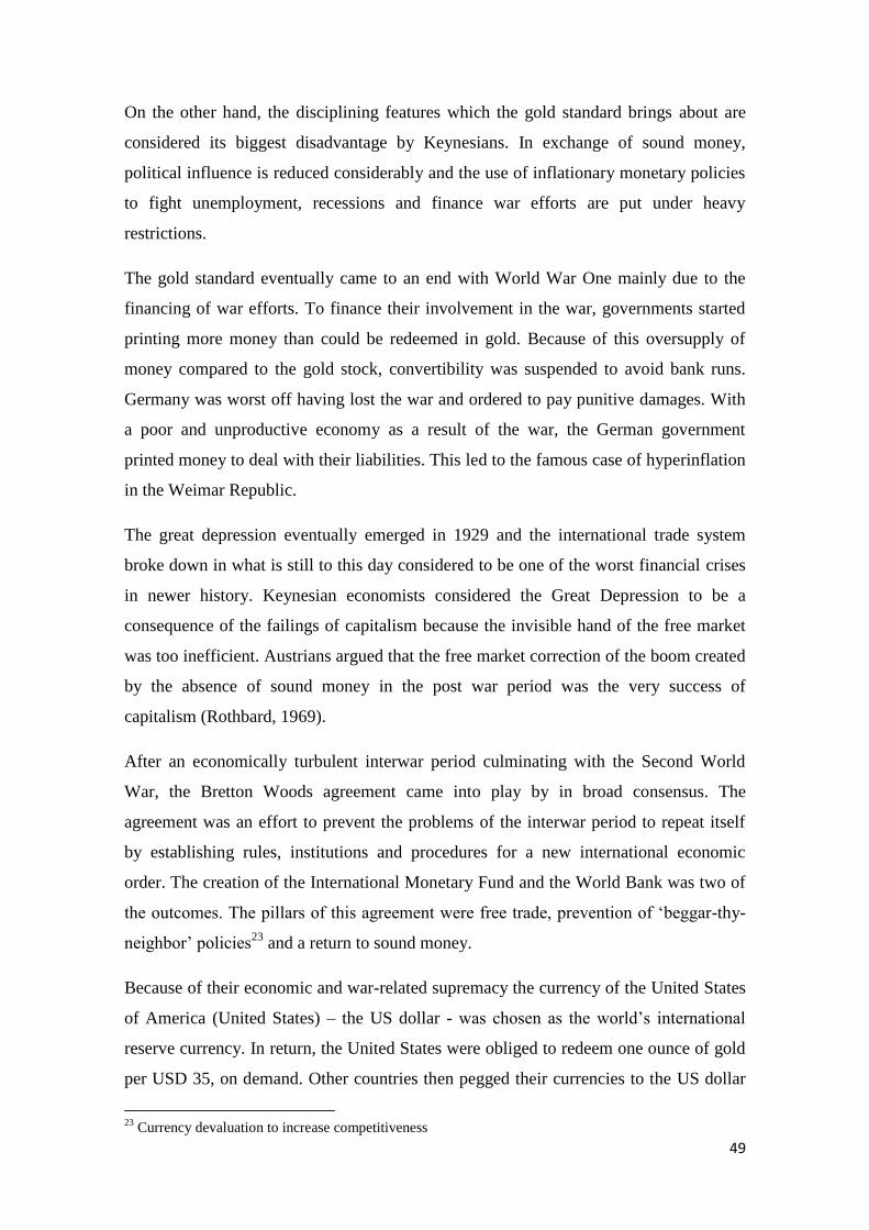
49

On the other hand, the disciplining features which the gold standard brings about are

considered its biggest disadvantage by Keynesians. In exchange of sound money,

political influence is reduced considerably and the use of inflationary monetary policies

to fight unemployment, recessions and finance war efforts are put under heavy

restrictions.

The gold standard eventually came to an end with World War One mainly due to the

financing of war efforts. To finance their involvement in the war, governments started

printing more money than could be redeemed in gold. Because of this oversupply of

money compared to the gold stock, convertibility was suspended to avoid bank runs.

Germany was worst off having lost the war and ordered to pay punitive damages. With

a poor and unproductive economy as a result of the war, the German government

printed money to deal with their liabilities. This led to the famous case of hyperinflation

in the Weimar Republic.

The great depression eventually emerged in 1929 and the international trade system

broke down in what is still to this day considered to be one of the worst financial crises

in newer history. Keynesian economists considered the Great Depression to be a

consequence of the failings of capitalism because the invisible hand of the free market

was too inefficient. Austrians argued that the free market correction of the boom created

by the absence of sound money in the post war period was the very success of

capitalism (Rothbard, 1969).

After an economically turbulent interwar period culminating with the Second World

War, the Bretton Woods agreement came into play by in broad consensus. The

agreement was an effort to prevent the problems of the interwar period to repeat itself

by establishing rules, institutions and procedures for a new international economic

order. The creation of the International Monetary Fund and the World Bank was two of

the outcomes. The pillars of this agreement were free trade, prevention of „beggar-thy-

neighbor‟ policies23

and a return to sound money.

Because of their economic and war-related supremacy the currency of the United States

of America (United States) – the US dollar - was chosen as the world‟s international

reserve currency. In return, the United States were obliged to redeem one ounce of gold

per USD 35, on demand. Other countries then pegged their currencies to the US dollar

23

Currency devaluation to increase competitiveness

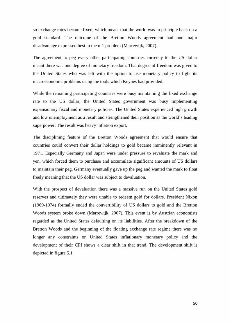
50

so exchange rates became fixed, which meant that the world was in principle back on a

gold standard. The outcome of the Bretton Woods agreement had one major

disadvantage expressed best in the n-1 problem (Marrewijk, 2007).

The agreement to peg every other participating countries currency to the US dollar

meant there was one degree of monetary freedom. That degree of freedom was given to

the United States who was left with the option to use monetary policy to fight its

macroeconomic problems using the tools which Keynes had provided.

While the remaining participating countries were busy maintaining the fixed exchange

rate to the US dollar, the United States government was busy implementing

expansionary fiscal and monetary policies. The United States experienced high growth

and low unemployment as a result and strengthened their position as the world‟s leading

superpower. The result was heavy inflation export.

The disciplining feature of the Bretton Woods agreement that would ensure that

countries could convert their dollar holdings to gold became imminently relevant in

1971. Especially Germany and Japan were under pressure to revaluate the mark and

yen, which forced them to purchase and accumulate significant amounts of US dollars

to maintain their peg. Germany eventually gave up the peg and wanted the mark to float

freely meaning that the US dollar was subject to devaluation.

With the prospect of devaluation there was a massive run on the United States gold

reserves and ultimately they were unable to redeem gold for dollars. President Nixon

(1969-1974) formally ended the convertibility of US dollars to gold and the Bretton

Woods system broke down (Marrewijk, 2007). This event is by Austrian economists

regarded as the United States defaulting on its liabilities. After the breakdown of the

Bretton Woods and the beginning of the floating exchange rate regime there was no

longer any constraints on United States inflationary monetary policy and the

development of their CPI shows a clear shift in that trend. The development shift is

depicted in figure 5.1.

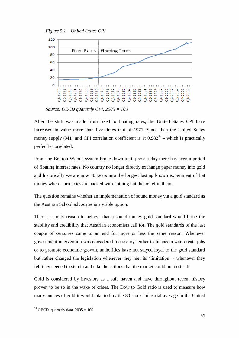
51

Figure 5.1 – United States CPI

Source: OECD quarterly CPI, 2005 = 100

After the shift was made from fixed to floating rates, the United States CPI have

increased in value more than five times that of 1971. Since then the United States

money supply (M1) and CPI correlation coefficient is at 0.98224

- which is practically

perfectly correlated.

From the Bretton Woods system broke down until present day there has been a period

of floating interest rates. No country no longer directly exchange paper money into gold

and historically we are now 40 years into the longest lasting known experiment of fiat

money where currencies are backed with nothing but the belief in them.

The question remains whether an implementation of sound money via a gold standard as

the Austrian School advocates is a viable option.

There is surely reason to believe that a sound money gold standard would bring the

stability and credibility that Austrian economists call for. The gold standards of the last

couple of centuries came to an end for more or less the same reason. Whenever

government intervention was considered „necessary‟ either to finance a war, create jobs

or to promote economic growth, authorities have not stayed loyal to the gold standard

but rather changed the legislation whenever they met its „limitation‟ - whenever they

felt they needed to step in and take the actions that the market could not do itself.

Gold is considered by investors as a safe haven and have throughout recent history

proven to be so in the wake of crises. The Dow to Gold ratio is used to measure how

many ounces of gold it would take to buy the 30 stock industrial average in the United

24

OECD, quarterly data, 2005 = 100

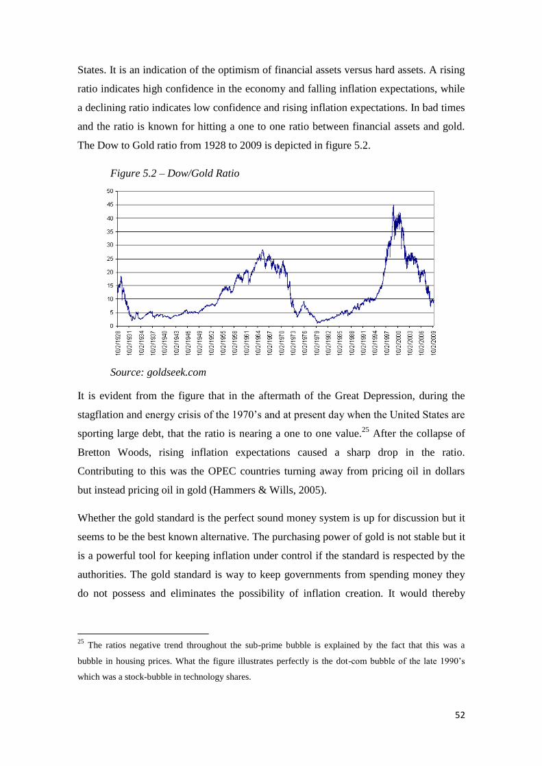
52

States. It is an indication of the optimism of financial assets versus hard assets. A rising

ratio indicates high confidence in the economy and falling inflation expectations, while

a declining ratio indicates low confidence and rising inflation expectations. In bad times

and the ratio is known for hitting a one to one ratio between financial assets and gold.

The Dow to Gold ratio from 1928 to 2009 is depicted in figure 5.2.

Figure 5.2 – Dow/Gold Ratio

Source: goldseek.com

It is evident from the figure that in the aftermath of the Great Depression, during the

stagflation and energy crisis of the 1970‟s and at present day when the United States are

sporting large debt, that the ratio is nearing a one to one value.25

After the collapse of

Bretton Woods, rising inflation expectations caused a sharp drop in the ratio.

Contributing to this was the OPEC countries turning away from pricing oil in dollars

but instead pricing oil in gold (Hammers & Wills, 2005).

Whether the gold standard is the perfect sound money system is up for discussion but it

seems to be the best known alternative. The purchasing power of gold is not stable but it

is a powerful tool for keeping inflation under control if the standard is respected by the

authorities. The gold standard is way to keep governments from spending money they

do not possess and eliminates the possibility of inflation creation. It would thereby

25

The ratios negative trend throughout the sub-prime bubble is explained by the fact that this was a

bubble in housing prices. What the figure illustrates perfectly is the dot-com bubble of the late 1990‟s

which was a stock-bubble in technology shares.

53

reduce misallocated capital and the market would be forced to correct itself on a

continuous basis, meaning that eventual bubbles become much smaller in magnitude.

If recessions and busts of asset bubbles are something politicians want to avoid it is

puzzling why they plant the seed for them to happen. There is an in for a penny, in for a

pound analogy to this, meaning that if the consequences of your initial actions are

something you don‟t want, you must either stop doing it or take the responsibility for it.

Instead of realizing this it seems that in recent history, the politicians only solution to

recessions have been to keep doing more of the same monetary policies while blaming

the problem on market failings. Recessions though are not the failings of free market

capitalism bit its main excellence.

Recessions are corrections in the markets where misallocated capital provided by an

increase in the money supply are removed. It might be sheer ignorance or it might be

the failings of the political system as we know it, but there is a clear foundation for a

causal effect of monetary expansion. That is; inflation, asset bubbles, recessions,

unemployment and finally eventual social unrest. Sound money could be a solution.

5.3. Economic Freedom

Sound money is just one pillar of the Austrian Schools view on macroeconomics. In

their quest to promote the most optimal approach to national economy they also

advocate for a number of other issues. These are; individual property rights under an

impartial rule of law, free trade for goods and services and limited government.26

The

levels of these are together categorized as economic freedom and worldwide there is a

strong relationship between economic freedom and people‟s quality of life.27

Economic Freedom is defined as each person having control over the fruits of their

labor and initiative in the pursuit of their dreams by means of their own free choice. In

an economically free society, individuals succeed or fail based of their individual merit.

Economic decision-making and allocation of recourses for production and consumption

is based on free and open competition to give everyone a fair chance to succeed.28

26

mises.org – What is Austrian Economics?

27 The Heritage Foundation –2011 index of Economic Freedom

28 Ibid.

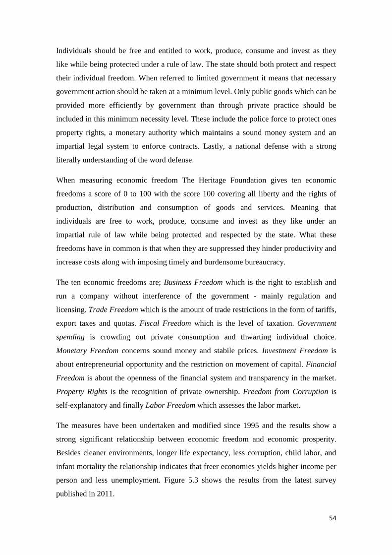
54

Individuals should be free and entitled to work, produce, consume and invest as they

like while being protected under a rule of law. The state should both protect and respect

their individual freedom. When referred to limited government it means that necessary

government action should be taken at a minimum level. Only public goods which can be

provided more efficiently by government than through private practice should be

included in this minimum necessity level. These include the police force to protect ones

property rights, a monetary authority which maintains a sound money system and an

impartial legal system to enforce contracts. Lastly, a national defense with a strong

literally understanding of the word defense.

When measuring economic freedom The Heritage Foundation gives ten economic

freedoms a score of 0 to 100 with the score 100 covering all liberty and the rights of

production, distribution and consumption of goods and services. Meaning that

individuals are free to work, produce, consume and invest as they like under an

impartial rule of law while being protected and respected by the state. What these

freedoms have in common is that when they are suppressed they hinder productivity and

increase costs along with imposing timely and burdensome bureaucracy.

The ten economic freedoms are; Business Freedom which is the right to establish and

run a company without interference of the government - mainly regulation and

licensing. Trade Freedom which is the amount of trade restrictions in the form of tariffs,

export taxes and quotas. Fiscal Freedom which is the level of taxation. Government

spending is crowding out private consumption and thwarting individual choice.

Monetary Freedom concerns sound money and stabile prices. Investment Freedom is

about entrepreneurial opportunity and the restriction on movement of capital. Financial

Freedom is about the openness of the financial system and transparency in the market.

Property Rights is the recognition of private ownership. Freedom from Corruption is

self-explanatory and finally Labor Freedom which assesses the labor market.

The measures have been undertaken and modified since 1995 and the results show a

strong significant relationship between economic freedom and economic prosperity.

Besides cleaner environments, longer life expectancy, less corruption, child labor, and

infant mortality the relationship indicates that freer economies yields higher income per

person and less unemployment. Figure 5.3 shows the results from the latest survey

published in 2011.

55

Figure 5.3 – Economic Freedom and GDP per capita - 2011

Source: heritage.org

The figure shows a clear relationship between the overall economic freedom score and

the level of income per capita. The results of this survey are coherent with the principles

of the Austrian School that less government, less regulation and more personal and

business freedom creates higher levels of prosperity.

This discussion section has only touched upon on the current global financial situation

but there is already a solid base for the arguments of the Austrian School. On the

concluding note that monetary policies creates business cycles which ends in painful

financial contractions, this discussion has presented the Austrian Schools answers to

avoiding this by readopting a system of sound money. Such a system would reduce

misallocation of capital and keep inflation from eroding the value of paper money. This

comes with a price of reduced political influence which removes the possibilities for

politicians to plant the seeds for financial bubbles. Whether this is a good or bad thing is

a question of ideological persuasion, but the „evidence‟ and current western world‟s

financial problems are in favour of the Austrian approach. Furthermore, the benefits of

this approach show a strong relationship with prosperity.

56

6. Conclusion

This thesis has presented the Austrian business cycle theory as an alternative to the

mainstream Keynesian business cycle approach. Whereas Keynesian theory is about

avoiding recessions or „busts‟ with monetary policy tools, the Austrian School wishes to

avoid the booms which precedes the busts.

The Austrian School blames the sole provider of legal tender – the central bank – for

creating inflation and business cycles. The case of endogeniety between the money

supply and inflation showed a remarkably clear indication of this relationship.

According to the Austrian School a business cycle is created by policy induced credit

injection to finance government spending and intervention. When money supply is

expanded the market interest rate falls below that of the natural time preference. At the

lower interest rate malinvestments are undertaken primarily in earlier stages of

production, causing a shift in the production structure, with the production structure

becoming more roundabout.

The lower interest rate also lowers incentives for saving with an increased demand for

consumer goods. A longer production structure paired with an increase in consumption

causes a shortage expressed in rising consumer prices. This makes later stage

investments relatively more attractive and the resource allocation is reversed, which

creates an increase in demand for credit. As a result the interest rate rises and initiates a

recession. The monetary authorities will try and avoid the recession by further injection

of credit, but will eventually run out of supply and let the interest rate go up. Investment

projects are abandoned and malinvestment liquidation begins.

Throughout the cycle the role of price signals are essential. Every development happens

because of is a reaction to prices, being in the price of capital, relative prices of

production and consumer goods or the price of consumer goods itself.

The main hypothesis of this Austrian business cycle theory that monetary policies

causes business cycles, led to an empirical analysis of the three Scandinavian countries;

Denmark, Norway and Sweden. Based on the theoretical framework of Bismans &

Mougeot (2009) this framework offers to analyze the non-empirical proposition of the

Austrian business cycle in an empirical manner.

57

Three variables; the ratio of consumption expenditure to investment expenditure, the

term spread and the ratio of consumption price index to production price index, were

regressed on the dependent variable approximating the Austrian business cycle – the

ratio of actual GDP to natural real GDP. The results show that the term spread and the

consumption to investment expenditure ratio have significant impact on aggregate

economic activity, whereas the relative price ratio does not. In line with the Austrian

business cycle theory, the influence of the two significant variables is expected to have

a negative effect which is confirmed by the negative signs of the coefficients in the

model.

This leads to the conclusion that an increase in the ratio of consumption expenditure to

investment expenditure has a negative impact on the ratio of actual real GDP and

natural real GDP. When consumption expenditure grows relative to investment

expenditure it means that the difference between actual real GDP and natural real GDP

is reduced. This corresponds with the Austrian business cycle theory, where the

expansionary phase begins with a relative increase in capital goods production, followed

by a later increase in consumption goods production. When the expansionary phase

comes to an end and the recession begins the opposite is true for the GDP ratio,

resulting in liquidation of malinvestments.

With regards to the term spread an increase in the approximated variable means a

decrease in the ratio of actual real GDP to natural real GDP. According to the Austrian

business cycle theory, monetary expansion lowers the short term interest rate which in

turn widens the gap between the long term rate and the short term rate. The model in the

present analysis reflects this since an increase in the term spread lowers the difference

between actual real GDP and natural real GDP. This brings real economic activity to

accelerate compared to its natural state until the short term market interest rate

converges to its natural level.

The acceptance of the Austrian business cycle hypothesis in this paper has added three

countries to the pool of analyzed countries as well as a regional analysis of Scandinavia

where the hypothesis apply. The remaining being the dominant economies of the United

States, Britain, France and Germany. This makes the Austrian approach relevant in

Scandinavia as well as in the tree major economies of Europe and most importantly the

issuer of the world‟s dominant reserve – the United States.

58

As a result of Keynesian policies, the United States have gone from being the world‟s

leading creditor nation to being the world‟s leading debtor nation. Based on the

sophisticated theories of Keynes the inflationary policies carried out over the last 50

years have today resulted in real risk of a collapse of the currency the world considers

its official reserve. At least that is what economists of the Austrian School are

projecting, if this use of inflationary credit injections continues. The worrying factor is

that they have been fairly spot-on about their projections in the past.

The Austrian School proposes the implementation of sound money as a solution keep

inflation under control. Sound money, if done correct, is a disciplining measure but it

comes with a price of less government control. A system of sound money have in recent

history been tried and tested but have not been a widespread success. History have

though not proven that is doesn‟t work as a disciplining device, instead it have shown

that the legislation around it have been changed to accommodate the use of Keynesian

monetary policies. First in the turbulent war-era in the beginning of the 20th

century -

which to some extend can be excused, but also in the breakdown of the Bretton Woods.

This came to an end because a fear of inflation caused a run of the United States gold

reserves. The solution was to let exchange rates float and discard the disciplining

measure that the security of gold is. After this breakdown the inflationary trend shifted

upwards. History has also shown that despite of a lack of a sound money gold standard,

the price of financial assets and gold converge in uncertain times, which there is a clear

indication of as this is written.

Sound money paired with limited government and economic freedom are the main

pillars of the Austrian schools economic paradigm. The Heritage foundation‟s analysis

of the connection between the degrees of economic freedom shows a strong relationship

between economic freedom and prosperity. Other positive side effects of this are cleaner

environments, longer life expectancy and less corruption, child labor, and infant

mortality.

59

List of References

Publications

ABEL, A. & BERNANKE, B. (1992). Macroeconomics. Addison-Wesley

BISMANS, F. & MOUGEOT, C. (2009). Austrian Business Cycle Theory: Empirical

Evidence. Springer

BLANCHARD, O. (2003). Macroeconomics. Prentice Hall, 3rd

edition

CHOI, I. (2001). Unit Root Tests for Panel Data. Journal of International Money and

Finance, April 2001, Vol. 20, Issue 2, 249-272.

EBELING, R. (1978). The Austrian Theory of the Trade Cycle. Center for Libertarian

Studies

FERGUSON, N. (2008). The Ascent of Money: A Financial History of the World. The

Penguin Press

GARRISON, R. (2001). Time and Money: The Macroeconomics of Capital Structure.

Routledge

HAMMERS, D. & WILLS, D. (2005). The end of Bretton Woods and the oil price

shocks of the 1970’s. The Independent Review, Spring 2005, Vol. 9, Issue 4: 501-511.

HERBENER, J. (1991). Ludwig von Mises and the Austrian School of Economics. The

Review of Austrian Economics, Vol. 5, No. 2 (1991): 33-50.

HODRICK, R. & PRESCOTT, E. (1997). Post-war U.S. Business Cycles – An

Empirical Investigation. Journal of Money, Credit and Banking, February 1997, Vol.

29, No. 1: 1-16.

HOPPE, H. (1995). Economic Science and the Austrian Method. The Ludwig von Mises

Institute

JOHNSON, L., LEY, R. & CATE, T. (2004). The Concept of Equilibrium: A Key

Theoretical Element in Keynes’ Revolution. Atlantic Economic Journal, September

2004, Vol. 32, Issue 3: 221-231.

KEYNES, J. (1936). The General Theory of Employment, Interest and Money.

Macmillan Cambridge University Press, for Royal Economic Society

KEELER, J. (2001). Relative Prices and the Business Cycle. Mises Institute

KIRZNER, I. (1997). Entrepreneurial Discovery and the Competitive Market Process:

An Austrian Approach. Journal of Economic Literature, March 1997, Vol. 35: 60-85.

60

KOROTAYEV, A. & TSIREL, S. (2010). A Spectral Analysis of World GDP

Dynamics. Structure and Dynamics, 2010. Vol. 4, Issue 1.

GARRISON, R. (2001). Time and Money: The Macroeconomics of Capital Structure.

Routledge

GILCHRIST, S. & WILLIAMS, J. (2000). Putty-Clay and Investment: A Business

Cycle Analysis. Journal of Political Economy, October 2000, Vol. 108, No 5.

MARREWIJK, C. (2007). International Economics. Oxford University Press

MISES, L. (1912). The Theory of Money and Credit. New Haven. Yale University Press

MISES, L. (1951). Inflation: An Unworkable Fiscal Policy. Mises Institute

MULLIGAN, R. (2006). An Empirical Examination of Austrian Business Cycle

Theory. The Quarterly Journal of Austrian Economics, Vol. 9, No 2: 69-93.

OBSTFELD, M. (2001). International Macroeconomics: Beyond the Mundell-Fleming

Model. International Monetary Fund, Vol. 47

PARKIN, M, POWELL, M & MATTHEWS, K. (1997). Economics. Addison-Wesley,

3rd

edition

PENATI, A. (1985). Government Spending and the Real Exchange Rate. University of

Pennsylvania, September 1985.

ROTHBARD, M. (1969). Economic Depressions: Their Cause and Cure. The Ludwig

von Mises Institute

SCHIFF, P. (2010). How an Economy Grows and why it Crashes. Wiley

SCHIFF, P. (2009). Crash Proof 2.0. Wiley

WOOLDRIDGE, J. (2006). Introductory Econometrics: A Modern Approach.

Thomson, 3rd

edition

61

Web pages

www.bis.org – Basel III

www.cia.cov – World Fact Book

www.goldseek.com – The Dow/Gold Ratio Will Decline Further

www.heritage.org – Economic Freedom

www.mises.org - Various

www.nber.org – Business Cycle Dating Procedure

www.oecd.org - System of composite leading indicators

Data Sources

Eurostat - http://epp.eurostat.ec.europa.eu/portal/page/portal/statistics/search_database

OECD- http://stats.oecd.org/Index.aspx

Statistical software

StataCorp. 2009. Stata Statistical Software: Release 11. College Station, TX: StataCorp

LP.

http://www.bis.org/

http://www.cia.cov/

http://www.goldseek.com/

http://www.heritage.org/

http://www.mises.org/

http://www.nber.org/

http://www.oecd.org/

http://epp.eurostat.ec.europa.eu/portal/page/portal/statistics/search_database

http://stats.oecd.org/Index.aspx

Austrian Business Cycle Theory Evidence from...

Documents

Transcript of Austrian Business Cycle Theory Evidence from...