Australian School of Business Working...
53
www.asb.unsw.edu.au Last updated: 18/09/12 CRICOS Code: 00098G Australian School of Business Research Paper No. 2011 ECON 08 Does Coresidence Improve an Elderly Parent’s Health? Meliyanni Johar Shiko Maruyama This paper can be downloaded without charge from The Social Science Research Network Electronic Paper Collection: http://ssrn.com/abstract=1917206 Australian School of Business Working Paper
Transcript of Australian School of Business Working...
www.asb.unsw.edu.au
Last updated: 18/09/12 CRICOS Code: 00098G
Australian School of Business Research Paper No. 2011 ECON 08 Does Coresidence Improve an Elderly Parent’s Health? Meliyanni Johar Shiko Maruyama This paper can be downloaded without charge from The Social Science Research Network Electronic Paper Collection: http://ssrn.com/abstract=1917206
Australian School of Business
Working Paper

1
Does Coresidence Improve an Elderly Parent’s Health?
Meliyanni Johar*
Economics Discipline Group
University of Technology Sydney
Po Box 123. Broadway
NSW 2007 Australia
Phone: +61 2 9514 7742
Fax: +61 2 9514 7722
Email: [email protected]
Shiko Maruyama
School of Economics
University of New South Wales
Sydney, NSW 2052 Australia
Phone: +61 2 9385 3386
Fax: +61 2 9313 6337
Email: [email protected]
*Corresponding author

2
Does Coresidence Improve an Elderly Parent’s Health?
Abstract
It is generally believed that intergenerational coresidence by elderly parents and adult
children provides old-age security for parents. Though such coresidence is still the most
common living arrangement in many countries, empirical evidence of its benefits to
parental health is scarce. Using Indonesian data and a program evaluation technique that
accounts for non-random selection and heterogeneous treatment effect, we find robust
evidence of a negative coresidence effect. We also find heterogeneity in the coresidence
effect. Socially active elderly parents are less likely to be in coresidence, and when they
do live with a child, they experience a better coresidence effect.
Keywords: Intergenerational coresidence, informal care, elderly health, treatment effect, factor structure model
JEL codes: I12, J1, C31
Funding: This research is supported by the Australian Research Council Discovery Project Grant DP110100773.

3
1. Introduction
It is widely assumed that living with adult children improves the health outcomes of
elderly parents through the provision of valuable family support. Arguably, coresidence
is the most comprehensive form of informal care, offering immediate instrumental,
emotional, and financial assistance. For generations, intergenerational coresidence has
been relied upon to protect the welfare of elderly parents, particularly in developing and
middle-income countries where public support systems for the elderly are
underdeveloped.
Despite the prevalence of informal care by adult children and its indisputable role
in today’s aging societies (e.g., OECD, 2005), solid empirical evidence of the presumed
beneficial role of coresidence with a child is scarce. On the contrary, nationally
representative data sets from numerous countries (e.g., the US, Japan, China, and
Indonesia) and many recent studies both show worse health outcomes for parents in
intergenerational coresidence than for parents living independently.
Researchers have discussed various pathways through which intergenerational
coresidence may affect parental health negatively. Elderly parents may transfer their
resources to adult children (Cameron and Cobb-Clark, 2001; Schroder-Butterfill, 2003;
Johar and Maruyama, 2011). Excessive reliance and caregiving burden on children may
reduce elderly parents’ incentive to invest in their health to extend their life (Maruyama,
2012). Economic development and population aging may have reduced the supply of
family support by adult children relative to its demand, which leads to tension and
conflict between generations and weakens the bargaining position of elderly parents
(Asis et al., 1995; Hermalin, 2000; Giles et al., 2003; Lachs and Pillemer, 2004; Zhang,
2004; Chan, 2005; Newberry, 2010; Teo, 2010). Whether the negative effect of
4
intergenerational coresidence dominates or not has significant policy implications,
especially for countries that expect to rely on family informal care in the foreseeable
future.
This paper aims to advance the literature by separating the real causal effect from
various confounding factors. We use the Indonesian Family Life Survey (IFLS). The
population of interest is elderly individuals who have at least one adult child. Verifying
whether the undesirable correlation is indeed causal is a challenging empirical task
because of the absence of experimental data. We follow the program evaluation
literature. In our setup, coresidence by an elderly parent and an adult child is referred to
as the ‘treatment’. The treatment group consists of elderly parents who live with a child
and the control group consists of elderly parents who have a child but do not live with a
child. The outcome of interest is parental health status and survival.
There are three classes of confounding factors that prevent us from applying a
simple regression framework: (1) reverse causality, (2) non-random selection, and (3)
heterogeneity in the treatment effect. Reverse causality concerns the possibility that
coresidence occurs in response to the deterioration of parental health. To mitigate the
potential bias due to reverse causality, we use the panel structure of the IFLS. We use
the most recent two waves of the IFLS, IFLS3 (2000) and IFLS4 (2007), and focus on
the health and survival outcome after seven years, conditional on health and coresidence
status in the base period. To address non-random selection and heterogeneity, we
employ the factor structure model of Aakvick, Heckman, and Vytlacil (2005). This
model provides a flexible yet parsimonious and tractable specification that allows us to
correct for non-random selection into coresidence and to accommodate heterogeneity in

5
the coresidence effect. These confounding factors, while common, have never been
adequately addressed by previous studies on this topic.
Non-random selection, especially selection by unobservable factors, may lead to a
significant bias. Even after controlling for observed characteristics, coresiding parents
may possess very different characteristics from non-coresiding parents, and these
differences may result in different health outcomes. For example, the parents who are
more likely to coreside may also be healthier, even after controlling for observed health
status, thereby biasing the coresidence effect estimate upward.
Heterogeneity in the treatment effect is another concern receiving increasing
attention in the program evaluation literature. In our case, it is reasonable to suspect that
the coresidence effect would vary by various family characteristics such as health status,
economic status, living environment, and closeness among family members. Suppose
families experience heterogeneous effects of equal magnitude in opposite directions.
Then the resulting overall effect averages zero, and in a homogeneous treatment effect
framework, an econometrician will incorrectly conclude that coresidence has no sizable
effect on all parents. Furthermore, by examining the extent and patterns of
heterogeneity, we can better understand the mechanism behind the coresidence effect
and offer relevant input to policymakers.1
For our rich, flexible model, identification is a major concern. We employ two
identification strategies. First, we exploit the richness of the IFLS to provide exogenous
determinants of coresidence decision (instruments) utilizing Indonesia’s multicultural
background. Indonesia comprises over 300 distinct ethnolinguistic groups with their
own traditional rules and practices, called adat. Adat influences a wide range of aspects
1 See Basu (2011) for a discussion of the importance of heterogeneous treatment effect for policies.
6
of an Indonesian’s life from birth- to death-related matters, including the coresidence
decisions of families. The IFLS records the most prevalent patterns of adat at the
community level. We use a collection of adat information to fully exploit exogenous
variation in the adat data and to enhance the efficiency of our empirical estimates.
Second, we extend the binary outcome framework of Aakvick, Heckman, and
Vytlacil (2005) by allowing for a five-categorical ordered outcome, combining four-
categorical self-assessed health information with the survival status. The original
Aakvick, Heckman, and Vytlacil model simultaneously estimates three binary-outcome
equations for selection, outcomes under treatment, and outcomes in non-treatment, in
which the correlation among three equations is fully parameterized through an
unobservable factor; thus the identification of this model is more challenging than
standard bivariate binary models. Our extension to the ordered framework allows us to
fully utilize the health status information in data to aid identification, requiring only a
limited number of fairly reasonable extra assumptions. We find that this extension
greatly improves the stability and robustness of our empirical model.
Our results are summarized in three key findings. First, a descriptive data analysis
reveals significantly worse health outcomes of elderly parents in coresidence. The seven
year mortality rate is 5.3 percentage points higher for coresiding parents, while the data
shows no significant difference in baseline health between the coresidence and non-
coresidence groups.
Second, when we account for non-random selection by unobserved factors, the
estimated average treatment effect of coresidence on seven year survival is -0.100 with
a standard error of 0.078: in other words, if coresidence is randomly assigned to elderly
parents, their seven year survival rate will decrease by 10.0 percentage points, or 1.38

7
percentage points per year. This finding suggests that previous studies that do not
adequately deal with selection on unobservables overestimate the coresidence effect.
Although this point estimate comes with a wide confidence interval, a number of
sensitivity checks consistently show that a negative coresidence effect is robust and the
positive coresidence effect story is unlikely.
Third, the coresidence effect exhibits considerable heterogeneity. The estimated
coresidence effect on the treated is significant and strongly negative. The seven year
survival rate of elderly parents in coresidence in the base period would be 18.9
percentage points higher (2.5 percentage points per year) if they had lived
independently. Both observed and unobserved factors generate this heterogeneity. Part
of the heterogeneity is related to parents’ social interactions. Elderly parents who work
and are involved in community activities are less likely to be in coresidence, and if they
do live with a child, they tend to experience a better coresidence effect. Wealth has a
protective effect only if parents live without children. These results suggest that
excessive parent-child dependence contributes to the estimated negative coresidence
effect.
2. Literature and Indonesian Context
2.1. Existing Evidence of Coresidence Effect
A negative association between parental survival and coresidence with a child is found
in many survey data. Maruyama (2012) reports that the three year mortality rate for
Japanese parents over 65 who live with children is 3.6 percentage points higher than
that of parents who live without children. In China, Li et al. (2009) report that the two
year mortality rate for Chinese parents over 77 who live with a child is 5.3 percentage
8
points higher than the overall sample mortality rate. In Indonesia, based on IFLS3 and
IFLS4, we find that the seven year mortality rate of elderly parents over 60 is 5.3
percentage points higher if they live with a child. Higher mortality rates for parents in
coresidence are not unique to Asian countries. Our calculation using the US Health and
Retirement Study (HRS) 2006-2008 shows that the two year mortality rate for
coresiding parents over 65 is 4.6 percentage points higher than that of non-coresiding
parents.
The literature has accumulated a number of attempts to verify whether this
unconditional mean difference indeed reflects the true causal effect of coresidence.
Recent studies exploit the wider availability of panel data to address the reverse
causality problem, but their findings are mixed.2 On the one hand, a few studies from
the US find a positive coresidence effect. Silverstein and Bengtson (1991) find that a
tight parent-child relationship may reduce the mortality risk of elderly parents by
providing a buffer against parents’ social loss (e.g., loss of spouse) and social decline
(e.g., loss of social network). Liang et al. (2005) find that coresidence is positively
related to the functional status and cognitive functioning of non-married elderly. Studies
from China also find that elderly individuals who live with family members report
better subjective well-being than those living alone (Chen and Silverstein, 2000; Liu
and Zhang, 2004; Silverstein et al., 2006; Chen and Short, 2008).
On the other hand, numerous studies have found that coresidence has a negative
effect on parents. Li et al. (2009) focus on parents over 77 in China and find that elderly
parents in coresidence are more likely to have activities-of-daily-living (ADL)
limitations and are not less likely to die than parents living alone. In Japan, elderly 2 Most early studies, found in the gerontology, sociology, demography, and public health literatures, suffer from reverse causation because they rely mainly on cross sectional analysis (e.g., Pillemer and Suitor, 1991; Ng et al., 2004).

9
mothers are found to have more than double the risk of heart disease when they coreside
with children (Ikeda et al., 2009). They are also found to have higher mortality rates
when they are cared for by daughters than by a spouse (Nishi et al., 2010). In Singapore,
Chan et al. (2011) find severer depressive symptoms among elderly parents who live
with children than among parents who live with children and a spouse. Using data from
Israel, Walter-Ginzburg et al. (2002) find that elderly parents who live with children
have higher mortality risk than the lone elderly, especially than those who have
extensive social engagements.
To the best of our knowledge, Do and Malhotra (2012) and Maruyama (2012) are
the only studies that attempt to correct for selection on unobservables. Using an
instrumental variable technique, Do and Malhotra (2012) find that coresidence reduces
depressive symptoms among South Korean widowed elderly mothers. They use the
number of sons as an instrument for coresidence and argue that it is an appropriate
instrument in the Korean setting because it is related to traditional rules of coresidence
and should not directly affect parental health. Maruyama (2012) applies the same
empirical framework as the present study for Japanese data, and finds a significant,
negative treatment effect on the treated: the three year survival rate of elderly parents in
coresidence would be 8.9 percentage points higher if they lived independently.
2.2. Why Negative Coresidence Effect?
The old age security hypothesis argues that parents have a child and invest in the child’s
education and health so that the child will repay the parents in the future by providing
monetary and non-monetary transfers to the parent (e.g., Nugent, 1985). This motive is
particularly relevant in traditional societies that feature close family ties but lack a
reliable public support system. If children live with their elderly parents to provide old-

10
age support, coresidence is predicted to have a positive effect on parental health. Using
data in the late 1980s from rural Pakistan, Kochar (2000) finds evidence that elderly
parents’ labor supply decreases with their coresiding children’s income.
The literature discusses several mechanisms that overturn this prediction. First,
resource transfers, whether monetary or non-monetary, may flow from parents to
children in coresidence. Elderly parents in good health often remain in employment
even when they live with adult children (Keaseberry, 2001; Cameron and Cobb-Clark,
2001 and 2005). Parents with a regular income source such as a pension are particularly
prone to having dependants, and they often assume full-parenting responsibilities for
adult children and grandchildren (Schroder-Butterfill, 2003). Johar and Maruyama
(2011) find that most coresidence formation in Indonesia is motivated by the children’s
need rather than the parents’ need.
Second, coresidence may worsen parental health because excessive reliance and
coresidence burdens on children create disincentives for altruistic parents to invest in
their health to extend their life. Maruyama (2012) finds supporting evidence for this
hypothesis in Japanese families.
Third, children in coresidence may provide no support. Today’s economic
development and modernization erode traditional filial piety and the authoritarian
relationship between generations. This leads to elderly parents being at greater risk of
disrespect and neglect (Lachs and Pillemer, 2004; Newberry, 2010). Using data from
numerous countries, the literature has documented increasing evidence of internal
disagreements and conflicts in shared households due to the clash of values and
declining tolerance by the younger generation (Giles et al., 2003; Zhang, 2004).
Behind these three mechanisms is the weakened bargaining position of parents.

11
When demand for old-age support is large and supply of such support is small, the price
of old-age security is higher and thereby the coresidence effect is more likely to be
negative.
2.3. Indonesian Context
Indonesian society features a number of characteristics and time trends that contribute to
a weakened bargaining position for elderly parents. On the demand side of elderly
support, most Indonesian elderly parents still expect to live with their child. Indonesia
has a tradition of close family ties and intergenerational coresidence. This tradition was
emphasized and reinforced in the 1960s Suharto era as the family principle
(kekeluargaan): the father is the heart of the family and respectful children defer to the
decisions of the father (Teo, 2010). At the same time, public welfare support for the
elderly is underdeveloped. A pension is available almost exclusively for public servants
and retirees of large firms. When elderly individuals have no child or do not live with a
child, they live alone, with a spouse only, or with others such as siblings. These elderly
individuals may get support from immediate family, available relatives, close neighbors,
various charity organizations within the community, new marriage, or patronage from
previous employers. However, formal aged care as an alternative to family support is
not widely acceptable among Indonesians: families regard institutional care for elderly
parents as taboo. Most aged care homes are privately run and quite expensive, often to
meet the demand of affluent families. Consequently, the market for formal care is very
small and the reliance on informal care is expected to remain in the future.
The supply of informal elderly care increasingly has difficulty meeting demand.
The number of Indonesians aged 60 and over is estimated to increase steadily to 28.8

12
million by 2020, or 11 percent of total population, from the current level of 7 percent,3
implying that there will be a smaller number of children available for elderly parents to
rely on. As a result of the Family Planning Program in the 1970s, the total fertility rate
in Indonesia fell from 6 births per woman to 3 in 1990, then to 2.6 in 2000 and the rate
fell further to 2.25 in 2011.4 Consistent with population aging, the literature observes
the shift in the younger generation’s attitudes towards filial piety in developing
economies which have experienced rapid income growth and westernisation (Hermalin,
2000; Chan, 2005; Teo, 2010). Modernization also implies that there are increased
opportunities for children, and thus higher opportunity costs to their staying with elderly
parents.
These trends naturally cause a change in a parent’s bargaining power in family
decision-making, and indeed, existing studies show that Indonesian elderly parents
maintain a full parenting role, providing material and practical support to their children,
often without reciprocal support when it is needed (Cameron and Cobb-Clark, 2001;
Schroder-Butterfill, 2003). As a result, Indonesian elderly parents in coresidence may
well experience a negative coresidence effect.
3. Estimation
We adopt the factor structure model of Aakvik, Heckman, and Vytlacil (2005). This
framework provides a flexible yet parsimonious and tractable specification that yields
easily interpretable expressions for both non-random selection by unobservables and
heterogeneity in the coresidence effect. The original Aakvik, Heckman, and Vytlacil
model simultaneously estimates three binary equations for (1) selection, (2) treated
3 Source: ILO (http://www.ilo.org/jakarta/info/public/pr/WCMS_124484/lang--en/index.htm) 4 Source: CIA World Factbook (http://www.indexmundi.com/g/g.aspx?c=id&v=31)

13
outcomes, and (3) untreated outcomes. The identification of such a model is challenging
for us, because we only have instruments with limited exogenous variation. We extend
their binary outcome model by allowing for a five-categorical ordered outcome,
combining health status information with the survival outcome. The treatment is
coresidence. The treatment group is elderly parents who live with a child, while the
control group is elderly parents who have at least one surviving child and do not live
with a child. For each elderly parent i , let iD be an indicator variable for treatment
status: it takes 1 if the parent coresides with a child (or at least one child), and 0
otherwise. Let iY0 and iY1 be two potential outcomes for parent i after seven years in the
untreated ( 0iD ) and treated ( 1iD ) states, respectively. iY0 and iY1 are measured by
categorical subjective health which can take five possible values: 4 for very healthy, 3
for healthy, 2 for somewhat unhealthy, 1 for unhealthy, and 0 for death. In this
framework, it is assumed that iY0 and iY1 are defined for everyone, and that these health
outcomes are independent across parents.
As our dependent variables are all discrete, we employ a latent index framework.
The coresidence equation is specified as
(1) DiDii UZD * , otherwise 0 ; 0 if 1 * iii DDD
where iZ is a vector of observed characteristics that influence the family’s coresidence
decision, D denotes its associated parameters, and DiU is a random error term that
captures the unobserved costs of coresidence.5 *iD thus measures the net utility of
coresidence.
5 Following Aakvik, Heckman, and Vytlacil (2005), the error terms in the three equations are defined as costs instead of benefits, without loss of generality.
14
The health outcome equations for the untreated (j=0) and treated (j=1) states are
specified as follows:
(2) jijiji UXY * , 1 ,0j
,0 if 0
0 if 1
if 2
if 3
if 4
*
*1
1*
2
2*
3
3*
ji
ji
ji
ji
ji
ji
Y
Y
Y
Y
Y
Y
where iX is a vector of observed characteristics, j denotes its associated parameters,
jiU is an error term that captures unobserved health shocks, and 21, , and 3 are cut-
off parameters. The exclusion restriction is satisfied when ii ZX . The latent health
variable, *jiY , has a structural interpretation: if it is positive, parent i survives, and a
larger value indicates better health. The cut-off points govern which category parent i ’s
health falls into. Note that our extension of the original Aakvik, Heckman, and Vytlacil
model to incorporate health status information requires only a limited number of fairly
reasonable extra assumptions: death comes below the worst health status,6 and the cut-
off parameter values are the same across individuals and across the untreated and
treated states.7 The model makes no a priori assumption on the cardinality of health
status.
Following Aakvik, Heckman, and Vytlacil (2005), we assume that the error terms
in equations (1) and (2) are governed by the following normal factor structure:
6 This is a fairly standard assumption in the health economics literature (e.g. Grossman’s health capital model and the QALY weights literature). Also, beside mortality, subjective health is the most commonly used measure of individual health in the literature (Banks and Smith, 2011). Subjective health summarizes various aspects of individual health and has been found to be highly correlated with life expectancy and the prevalence of chronic diseases. 7 We assume that the four health categories provide a common metric for Indonesian elderly parents, at least approximately. Our approach is not appropriate if each parent perceives the categories and assesses their health in a significantly different way.

15
(3) ,DiiDiU ,000 iiiU and iiiU 111 ,
where each of the random terms 10 ,,, D is assumed to follow the i.i.d. standard
normal.8 This specification implies that
(4) ,),(Cov 00 UUD ,),(Cov 11 UUD and 1010 ),(Cov UU .
Estimation relies on the maximum likelihood method. The likelihood function has
the form
(5) N
i iiii dZXYDL1
, )( ),,|,Pr(
where is the standard normal probability density function. Let denote the standard
normal cumulative distribution function. The joint probability is given by:
(6) ),,,|Pr(),|Pr(),,|,Pr( iiiiiiiiii DXYZDZXYD
where
(7) ),(),|Pr( iDiii ZZD
and for 1 ,0j ,
),(),,|4Pr( 3 ijjiiiiji XjDXY
),()(),,|3Pr( 32 ijjiijjiiiiji XXjDXY
),()(),,|2Pr( 21 ijjiijjiiiiji XXjDXY
and ),()(),,|1Pr( 1 ijjiijjiiiiji XXjDXY
).(1),,|0Pr( ijjiiiiji XjDXY
To integrate i , a numerical approximation by Gauss-Hermite quadrature is used.
An advantage of using the factor structure model is that the mean treatment
parameter and the distributions of the treatment parameter can be obtained from the
estimated structural parameters. Let denote the treatment effect with regard to 8 The normality assumption guarantees the following standard assumptions: (i) ),( 0UU D
and ),( 1UU Dare
independent of ),( XZ ; (ii) ),( 10 YY have finite first moments; and (iii) 0)|1Pr(1 XD .

16
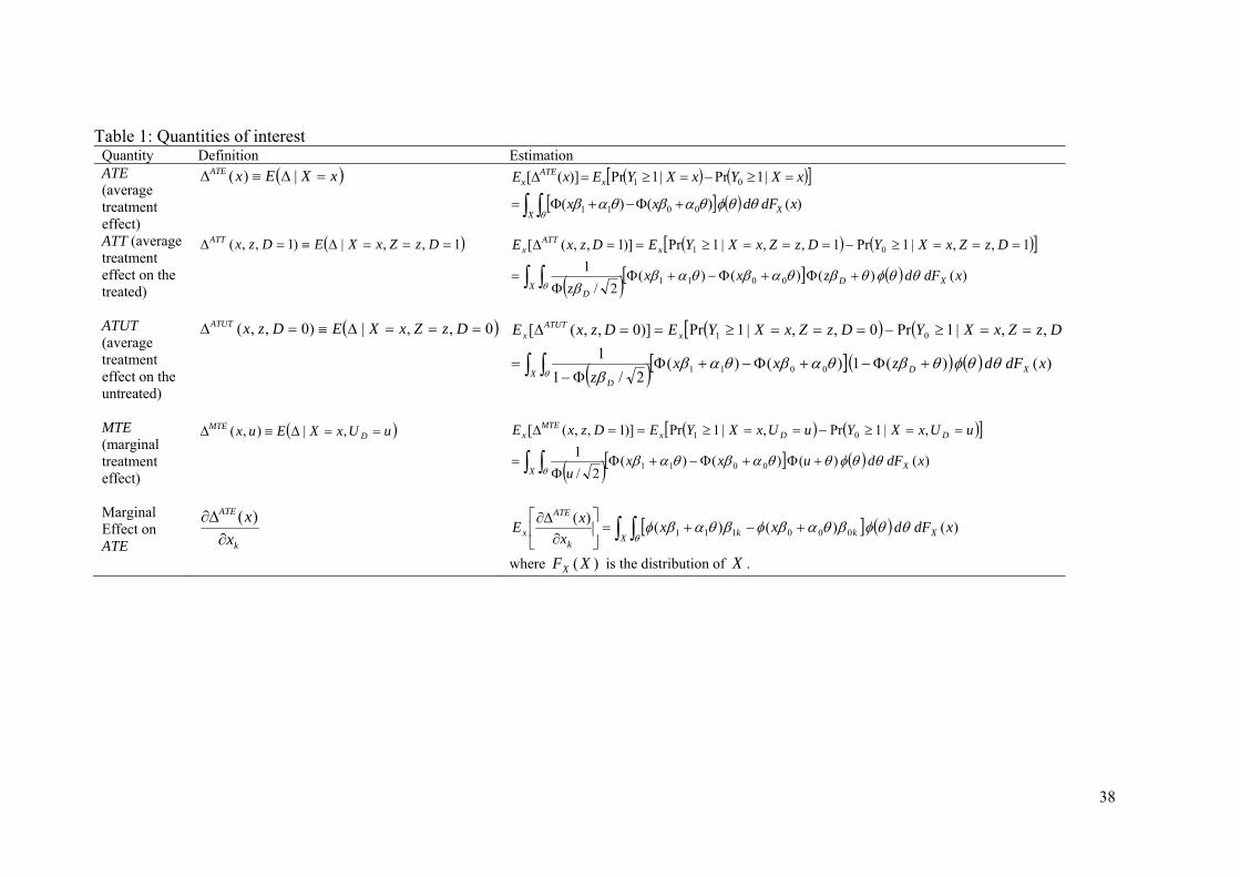
survival for a given parent: 1111 01 YY . Four quantities of interests are: (i) the
average treatment effect (ATE); (ii) the average treatment effect on the treated (ATT)
and on the untreated (ATUT); (iii) the marginal treatment effect (MTE); and (iv) the
marginal effect of covariate kx on the ATE. Parameters (i) through (iii) measure the
average effect under different conditions. The ATE measures the average effect for a
parent chosen at random from the population. The ATT and ATUT measure the average
effect for a parent who is in coresidence and for a parent who is not in coresidence,
respectively. The MTE measures the average effect for a parent who is indifferent to
coresidence for given values of covariates. Specifically, it is the average effect for a
parent who is indifferent between coresiding and living independently if the (observed)
instrument is externally set so that uUZ DD (Equation (1)). A high value of u is
associated with a high net cost of coresidence. For small values of u, the MTE is the
average effect for a parent with unobserved characteristics that make the parent more
likely to choose coresidence. The overall expected value of MTE is ATE. The marginal
effect of observed characteristics on the ATE, (iv), tells us how the treatment effect
varies across covariates and is informative in inferring the mechanism underlying the
causal effect. Table 1 summarizes these parameters. We also compute the distributional
parameters for the events, 0 ,1 , and 1 . The probability of a positive treatment
effect, xXYYxX |0 ,1Pr|1Pr 01 is calculated as follows:
(8) dxxxXYY 1|0 ,1Pr 001101 .
X|0Pr and X|1Pr are calculated in the same manner.
[Insert Table 1]
17
Summary estimates of all quantities of interest are found by integration over the
empirical distribution of X . Standard errors are computed using the delta method.
4. Data
The data is derived from the Indonesia Family Life Survey (IFLS), a nationally
representative longitudinal study of Indonesian households, collected by the RAND
Corporation in collaboration with several Indonesian universities. The IFLS began in
1993 and follow-ups were administered in 1997, 2000, and 2007. The reliability of the
IFLS is documented in Thomas et al. (2001). We use the latest two waves of the IFLS:
IFLS3 (2000), which provides base year information, and IFLS4 (2007), which provides
health outcome information seven years later.9 The population of interest is elderly
parents: individuals aged 60 years or older who have at least one adult child (aged 15 or
above) in the base year.10 We exclude elderly parents whose spouse is younger than 55
to avoid the complication due to the presence of a non-elderly parent. Both the husband
and wife are included as two observations when both of them are aged 60 or older. Our
final sample consists of 1,768 elderly parents, of whom 69.8 percent lived with at least
one child in 2000.
The dependent variable is a five-category health outcome variable that takes a
value of 0 if an elderly parent dies within seven years (between IFLS3 and IFLS4). If
an elderly parent survives, the dependent variable takes a value between 1 and 4,
corresponding to the four self-assessed health levels. The distribution of the health
9 Though the inclusion of the transition from IFLS1 (1993) to IFLS3 (2000) substantially increases the number of observations, we do not take this approach because of a substantial missing value problem in IFLS1. 10 This age threshold has been used by previous Indonesian studies (Hermalin, 2000; Cameron and Cobb-Clark, 2001; Johar and Maruyama, 2011). The child may be a biological child, a stepchild, or an adopted child. Our definition of elderly parents does not include individuals who have only a child-in-law.

18
outcome variable is shown in Table 2. It is lumpy around the two middle categories.
Respondents appear to be conservative about placing themselves at the extremes of the
health distribution. The seven year mortality rate is 31.4 percent in the sample or 4.0
percent per annum. The high mortality rate reflects the shorter life expectancy in
Indonesia.
[Insert Table 2]
Table 2 also compares the distributions of health outcomes by coresidence status.
The raw data clearly shows the negative association between parental health and
coresidence. Such negative association could be observed if parents with worse health
conditions were more likely to be in coresidence. In Indonesian families, however, such
reverse causation is unlikely. The binary baseline health status reported in the last line
of Table 2 indicates no substantial difference by coresidence status. Figure 1 visualizes
the health outcome distribution by baseline subjective health status. The fact that the
negative relationship remains even if baseline health is controlled for suggests that a
negative causality runs from coresidence to parental health.
[Insert Figure 1]
Table 3 provides a description of all the variables used in this study. Individual
characteristics include age, sex, baseline health conditions, economic status, and the
presence and age of a spouse. For baseline health, we use self-assessed health and health
conditions. The latter is constructed as the first factor from a factor analysis based on
twelve health condition measures.11 Socio-economic status includes working status, the
11 The twelve measures are: time taken to sit and stand five times; two indicators for suffering from chest pain and persistent wounds; and the ability to perform a series of nine activities of daily life (ADL). The nine ADLs are: to carry a heavy load (e.g., a pail of water) for 20 meters; to sweep the house floor yard; to walk 5 kilometers; to draw a pail of water from a well; to bow, squat, or kneel; to dress without help; to stand up from a sitting position in a chair without help; to stand up from sitting on the floor without help; and to go to the bathroom without help.
19
presence of pension payments, education, ownership of the residential house, and
household wealth measured in deciles.12
[Insert Table 3]
The last group of variables in Table 3 are our instruments. We use a combination
of community-level and individual-level instruments. The community-level instruments
are constructed based on adat (traditional practices) regarding inheritance and living
arrangements. A community is the smallest administrative unit in Indonesia and consists
of 2,500 family heads on average.13 The IFLS contains 312 communities. Because
communities in Indonesia are often multicultural, a community does not uniquely
determine an adat, so the IFLS records the adat of the dominant ethnic group in the
community. For our purposes, we use the following adat variables: whether the parent’s
house is traditionally transferred to the child in coresidence when the parent dies;
whether inheritance is traditionally unequally distributed according to a child’s gender,
birth order, and provision of informal care; how inheritance is traditionally shared
among a bereaved family; and whether children live with parents after marriage.14 Each
adat variable is binary, and we use a collection of them to enhance efficiency by
exploiting exogenous variation from the data.
We argue that these adat variables are valid instruments. Adat affects a family’s
coresidence decision by altering social pressures and incentives. The tradition of
bequeathing a house to children, for example, puts extra pressure on parents to pass it
on to coresiding children, creating incentives for children to live with their parents.
12 Wealth includes real estate, vehicles, jewellery, household appliances, livestock, receivables, and savings. Deciles are computed using the full sample of the IFLS households. 13 Four administrative units in Indonesia from smallest to largest are: community or desa (village), kecamatan (district), kabupaten (municipality), and province (e.g. Jakarta). Today, there are 33 provinces, 497 kabupaten, over 6,500 kecamatan, and over 75,000 communities. 14 Adat information was collected only twice, in 1997 and 2007. We use the 1997 survey (IFLS2) as it is closer to IFLS3.
20
Despite modernization, adat is still relevant in Indonesian society; people are still afraid
to break the law in 80 percent of the communities. While the adat variables influence
the coresidence decisions of families, it is hard to imagine that adat directly improves or
worsens someone’s health, conditional on the baseline health and other covariates. In
various fields, area-level variations have been used as instruments by many previous
studies. A possible concern arises if inheritance rules influence the amount and quality
of informal care by altering children's incentive. In the Indonesian setting, however,
there is little room for children to behave in such a strategic way, because elderly
parents typically have very small non-property wealth to bequeath and houses are the
major asset to be inherited. As a house is an indivisible asset, the amount and quality of
care a coresiding child provides cannot substantially affect the level of inheritance the
child expects. We later provide several robustness checks to address this concern.
To reinforce the adat instruments, we also use two individual-level instruments:
(1) whether the respondent’s spouse was chosen by his/her parents, and (2) the number
of the children the respondent has. The former influences the coresidence decision
because if it is a family’s tradition to choose a son-in-law or daughter-in-law, the choice
ought to reflect the parents’ preferences for coresidence. The latter instrument affects
the coresidence decision because having more children increases the likelihood of
coresidence with a child. At the same time, these two instruments are unlikely to
directly affect a parent’s health transition, conditional on the baseline health.15
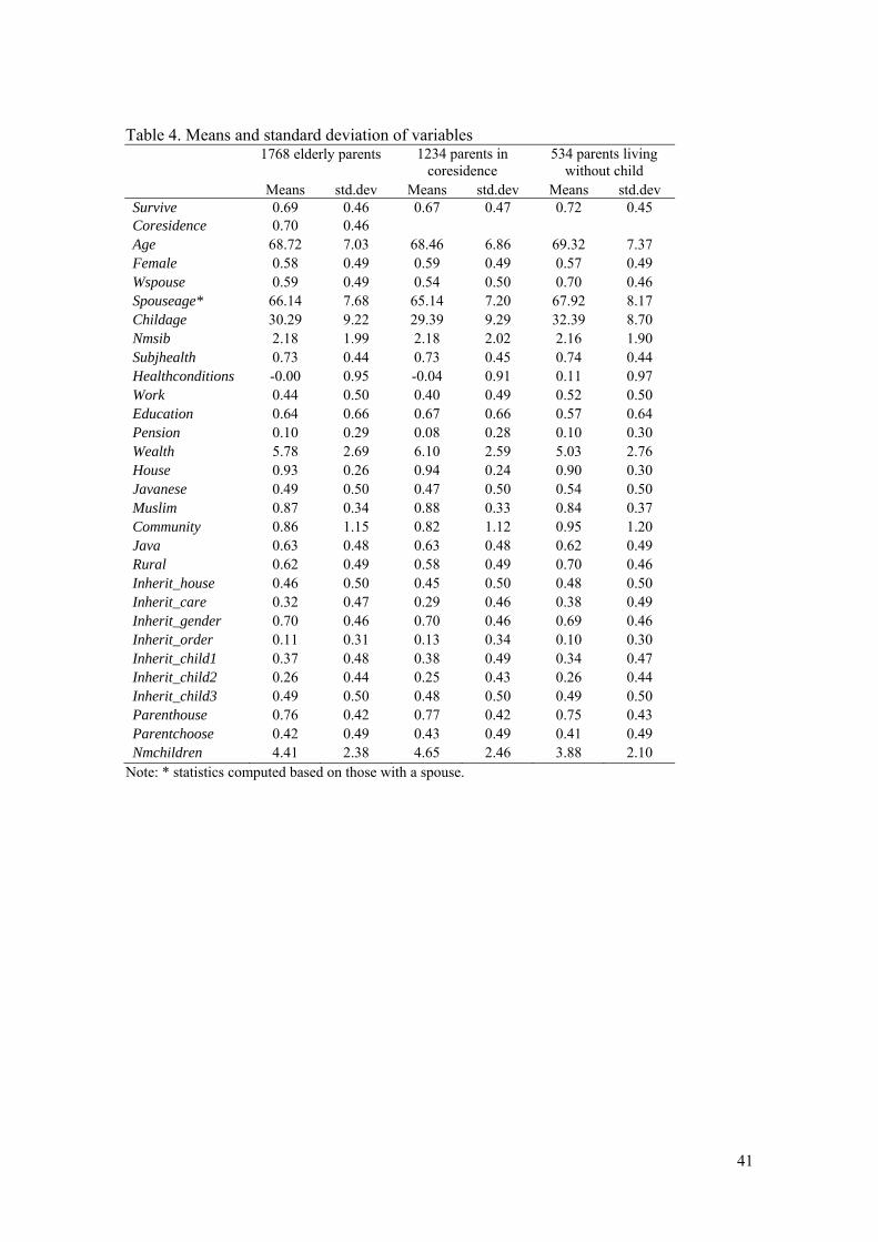
Table 4 provides descriptive statistics of all the covariates and instruments.
Parents in coresidence tend to be younger and do not live with a spouse, or live with a
15 The latter instrument violates the exogeneity condition if the presence of siblings affects how a child cares for his/her parents, as discussed in Bernheim et al.’s (1985) strategic bequest motive hypothesis. In the Indonesian setting, however, the strategic bequest motive appears to be limited, because of very little non-property wealth to bequeath.
21
younger spouse if married. Parents in coresidence also tend to have younger children,
greater wealth, and more children. They tend to live in a non-rented house and in
communities that traditionally reward children equally, regardless of the level of care
they provide, and in communities where parents have greater power in the marital
decision of their children. Both self-assessed health and health conditions show no
significant difference between the two groups at the base period, indicating that the
reverse causality explanation is highly unlikely.
[Insert Table 4]
5. Results
In this section, we first present simple linear survival models to outline characteristics
of the data and to discuss the validity of the instruments. We then report the results of
the full model. At the end of the section, we report a number of sensitivity tests and
discuss the robustness of our results.
5.1. Linear survival analysis
The dependent variable in the binary survival model is seven year survival; it takes a
value of one if the respondent is alive in 2007 and zero otherwise. Table 5 reports three
simple estimates of the coresidence effect: [1] the unconditional average effect; [2] the
average effect from a linear probability model (LPM); and [3] the average effect from a
linear probability model with instruments (LPM-IV).
[Insert Table 5]
The unconditional average effect shows that the seven year mortality rate for
parents in coresidence is 5.3 percentage points higher than for those who have a child
but live independently. The result is statistically significant at the 5 percent level. This

22
estimate may only reflect systematic differences between families in coresidence and
non-coresidence. Column [2] indicates a mild negative selection on observables: once
we control for observable characteristics, the average coresidence effect reduces to 3.6
percentage points and becomes insignificant. While a part of the unconditional mortality
difference by coresidence status can thus be attributed to variations in observables, more
than half of the gap still remains. When we also control for selection on unobservables,
as shown in column [3], the coresidence effect increases to 8.5 percentage points.
Although not significant, this increase indicates the presence of a positive selection bias
due to unobservables. Elderly parents with unobservable traits that contribute to their
survival probability — such as inherent health, mental strength, and strong family
altruism and reciprocity — are more likely to enter coresidence, after controlling for
observables. Later, when we extend the survival analysis by incorporating health
transition and allow for a heterogeneous coresidence effect, the coresidence effect is
more precisely estimated.
Standard tests support the validity of our instruments. In the first-stage regression,
the instruments are jointly significant (p-value = 0.00), indicating that they are strong
predictors of coresidence. 16 The overidentification test of the independence of all
instruments and the error term in the survival equation cannot be rejected at any
conventional significance level (p-value=0.353).
5.2. Coresidence equation
The full model estimates the coresidence equation and the two health outcome equations
simultaneously. Table 6 reports the coefficient estimates of the coresidence equation
16 The results are available on request.

23
(Equation (1)), which should be interpreted as correlation rather than causation, because
unobserved confounding factors may exist.
[Insert Table 6]
The statistical significance of many covariates confirms non-random selection
into coresidence. Coresidence is less likely for old couples and mothers. This is
consistent with existing Indonesian studies (Schroder-Butterfill, 2003; Johar and
Maruyama, 2011) and other studies from neighbouring Southeast Asian countries (Chan,
2005). Holding parental age constant, the parents of younger children are more likely to
coreside. Coresidence is also more likely when parents work, receive a pension, have
smaller wealth, own a house, engage in the community, and live in an urban area as a
non-Muslim. The two health variables have no significant power in explaining
coresidence; hence, it is not the baseline health gap that generates the negative
coresidence effect.
The results also confirm the significance of the instruments. Traditional practices
matter to the coresidence decision, illustrating the strong influence of cultural norms
and traditional customs in Indonesian families’ lives.
5.3. Health outcome equations
Table 7 reports the results of the two health outcome equations. In both states, younger
parents are more likely to have a better health outcome, and so are mothers, reflecting
the higher life expectancy of females. Naturally, subjective health and existing health
conditions at the baseline are strong predictors of health outcomes seven years later.
Work, a spouse, and community involvement lead to a better health outcome if parents
live with a child. Our tentative interpretation of these findings is the importance of
parents’ social interactions to avoid excessive reliance on coresiding children and

24
associated undesirable effects of coresidence. Wealth is another variable with a
significantly contrasting effect across the coresidence states: greater wealth improves
the health of parents only when the parent does not live with a child. While wealth
potentially protects health, it may attract more dependent children (Johar and Maruyama,
2011). The number of siblings has a significant protective effect only when a parent
lives without a child, suggesting the role that siblings may play as alternative care
providers in the absence of children.
[Insert Table 7]
Table 7 also reports estimates of the three cut-off points for ordered health
outcomes. These thresholds are relative to the threshold for death that is normalized to
zero. They are precisely estimated and have reasonable values. The large difference
between 2̂ and 3̂ reflects the fact that a very small share of parents answered that they
were “very healthy”. As a robustness check, we estimate a three-category model, in
which we aggregate “very healthy” and “somewhat healthy” into “healthy” and
“somewhat unhealthy” and “unhealthy” into “unhealthy”. Its results are fairly consistent
with the five-category model.17
The factor structure parameter, , enters the health outcome equations with the
coefficient parameters, 0 and 1 . Note that a model with no selection on
unobservables implies 010 . The estimates of 0 and 1 are reported in the row
after the constant term with the heading Factor( ). These parameters have different
signs, capturing heterogeneity in the treatment effect due to unobservables, although a
17 The results are available on request. We have also attempted binary outcome models which only focus on survival. While their results are generally consistent with our full model, estimates are sensitive to specifications, and convergence is often unstable.
25
model without selection cannot be formally rejected (they are not jointly significant:
Chi-squared statistics of 2.92 with a p-value of 0.23).
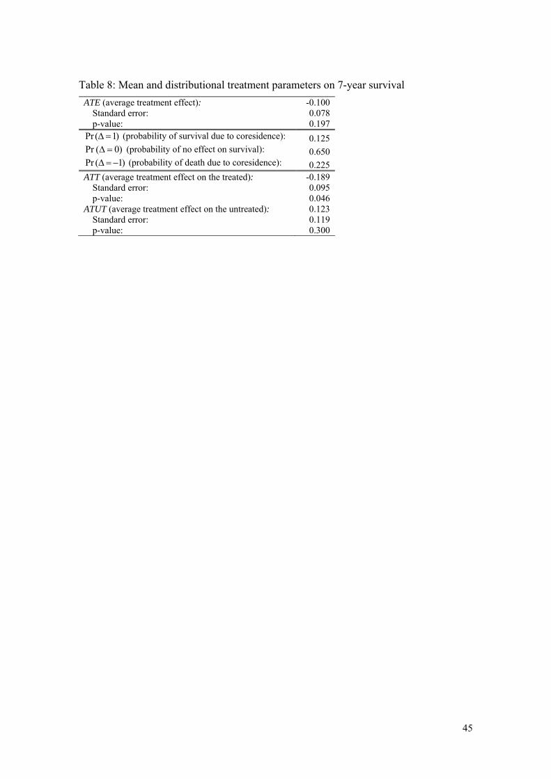
5.4. Treatment effects
The estimated treatment effect parameters are reported in Table 8. The ATE measures
the average effect of coresidence on the survival of a parent drawn randomly from the
entire elderly parent population. The ATE is estimated to be -0.100 with standard error
of 0.078. The point estimate implies an increase in seven year mortality rate by 10.0
percentage points, or 1.4 percentage points per annum. This result weakly indicates a
negative (average) causal effect of coresidence. It also indicates that a substantially
positive average coresidence effect is unlikely to exist. Compared with the linear binary
model with the same instruments (in Table 5), the size of the coresidence effect is
slightly larger, and incorporating health status outcomes improves precision.
[Insert Table 8]
The next rows in Table 8 present the distributional parameters of the ATE. They
illustrate that randomly assigning coresidence to parents would alter their health
outcomes in seven years as follows: 12.5 percent of them would avoid death due to
coresidence, 65.0 percent would not be affected by coresidence, and 22.5 percent would
die because of coresidence.
The ATT is the average effect on the treated population. As shown in Table 8, the
estimated ATT on mortality is significant at the 5 percent level and implies that if
parents in coresidence had not chosen to coreside, their seven year survival rate would
have been 18.9 percentage points higher (or 2.5 percentage points per annum). The
ATUT is estimated to be positive 0.123. These indicate heterogeneity in the coresidence

26
effect: elderly parents who were in coresidence in the base year are those who are prone
to suffer from an undesirable treatment effect.
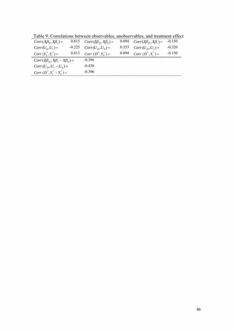
Heterogeneity in the coresidence effect can be attributed to observed and
unobserved factors. To illustrate the working of the factor structure model, Table 9
reports correlation estimates between observables, unobservables, and the treatment
effect. The first three rows provide correlations among the selection and health outcome
variables in terms of observed and unobserved factors. The two health outcome
equations ),( *1
*0 YY are strongly and positively correlated due to the strong positive
correlation of observable factors ),( 10 XX . The unobserved factors ),( 10 UU are
negatively correlated. The correlation between selection and health outcome exhibits
different signs across the coresidence and non-coresidence states. In terms of both
observables and unobservables, factors that induce coresidence are positively correlated
with factors that benefits health outcomes in the non-coresidence state, whereas the
factors that induce coresidence are negatively correlated with health factors in the
coresidence state. Taking these relationships altogether, the last three rows show the
negative relationship between coresidence and the coresidence effect, where both
observables and unobservables contribute to the negative relationship.
[Insert Table 9]
Figure 2 plots the point estimate of the MTE with its 95 percent confidence
intervals. The horizontal axis represents the value of DU , which is labelled by its
cumulative probability value. A higher value of DU implies a lower probability of
coresidence (see Equation (1)). The upward sloping MTE curve implies that in terms of
unobservables, parents who are more likely to be in coresidence (i.e. those who have a
small DU ) are more likely to experience a significant health decline under coresidence
27
than those who are less likely to coreside. This reflects the negative ),( 01 UUUCorr D .
Recall that in our notation, a larger value of )( 01 UU makes the coresidence effect
worse. Unobserved factors underlying the heterogeneous effect might capture the
dependence of children, parental altruism, other intergenerational relationship, or
unobserved physical or mental health disposition. In the present analysis, we are
agnostic about the underlying unobservables.
[Insert Figure 2]
Observables also generate heterogeneity in the coresidence effect, and they are
informative in inferring the mechanism underlying the causal effect. Table 10 reports
the marginal effects of observed characteristics on the ATE. Significant marginal effect
is found for only one variable – community engagement. Parents who have little
community engagement tend to be those who experience greater health deterioration
due to coresidence. The same relationship is found for working and marital status,
although with much lower significance. These findings indicate the importance of social
interaction to avoid an undesirable coresidence effect on parental health. Social
activities may help parents to avoid excessive dependence on coresiding children and
associated conflicts, by maintaining their mental well-being and subjective happiness.
The positive effect of social interactions may also come from changes in children’s
behavior. In small closed communities, more widely networked parents may generate
incentives to children to do well in their education and job, and to increase the attention
and care given to parents to maintain a good family image and avoid being labelled as

28
an ungrateful child.18 Consistent with our earlier discussion, parental wealth negatively
contributes to the coresidence effect, though it is not sharply estimated.
[Insert Table 10]
The use of ordered health outcomes allows us to compute the ATE on health
status. Table 11 shows the conditional ATEs, with associated unconditional transition
rates for reference. For parents who are healthy in the base year, coresidence lowers
their probability of becoming ‘very healthy’ by 5.17 percentage points and ‘somewhat
healthy’ by 8.92 percentage points. At the same time, their probability of health
deterioration into the two unhealthy states increases by 4.3 percentage points and their
probability of death increases by 9.14 percentage points. The baseline health status does
not affect the coresidence effect: coresidence similarly shifts the health outcome
distribution of those who are unhealthy in the base year downward.
[Insert Table 11]
5.5. Robustness of results
The estimated ATE and ATT are 10.0 and 18.9 percentage points, respectively (1.4 and
2.5 percentage points per annum). We argue that these large effects are not implausible.
We are concerned with the population aged 60 and above in Indonesia. The national life
expectancy at birth (at age 60) at this period is around 68.1 (77.4) years.19 The seven
year mortality rate for our sample is 31.4 percent (4.0 percent per annum), and the seven
year mortality rate for those above 80 is 60.1 percent (7.0 percent per annum). The
unconditional mean difference by coresidence status obtained from the raw data is
already as large as 5.3 percentage points (Table 5), and 11.0 percentage points if we
18 A reverse causation might be possible: parents limit their social interaction when taking care of their children occupies their time and resources. Disentangling the causal mechanism here is beyond the scope of this research. 19 Source: Medika Consulting, “Indonesia life expectancy history”, Indonesia (http://www.medika-consulting.com/website/26378/images/htmleditorfiles/INDONESIA-health-data-medikaconsulting.pdf).

29
only use those above 70. The distributional assumptions of the single factor structure
may be another source of the large ATT, because its functional form assumption
determines the way the heterogeneous treatment effect is distributed (Figure 2). The
implication of the one-factor structure assumption in our context is left for future
research.
At the same time, because we estimate a flexible model by relying on
community-level instruments and a number of econometric assumptions, the robustness
of our results may be of concern. To address this concern we provide a series of
sensitivity analyses to ensure the robustness of our results. First, we estimate our main
model with various sets of instrumental variables. We experiment with different
permutations of the instruments, including those used in our preferred model, two
additional adat variables, family-level variables (business assets and characteristics of
the house), and community-level time trend in the age structure and family size between
1993 and 2000. As shown in Table 12, the negative coresidence effect is robust; our
results are not driven by a particular instrument or by a particular combination of
instruments.20 Furthermore, we also estimate a variant of our preferred model in which
Inherit_care is included as one of the covariates, x, not an instrument. This is to address
to the concern that the inheritance rule that relates to the amount of care might influence
the amount and quality of care a child in coresidence provides. If this specific adat
influences care quality, it violates the exogeneity condition. The estimated results
confirm that this is not the case: the estimated ATE and ATT are almost the same as our
20 We do not include business assets and housing characteristics in our preferred model because of the concern about their validity. We do not employ the community-level time trend instruments either because some communities in our data have too few observations to accurately infer community level trends.

30
preferred model (–10.1 and –18.6, respectively), and the ATE does not vary by
Inherit_care.21
[Insert Table 12 here]
As another instrumental variable validation test, we study how our covariates
vary along our instruments. If the covariates in the health outcome equation and the
instruments always move together, this raises concerns about the instruments. Since we
have multiple instruments, we run a simple probit regression of coresidence on only the
instruments, generate a propensity score, and divide it into quartiles. At the 5%
significance level, we find that the propensity scores are: (1) balanced (statistically
indifferent) across top and bottom quartiles for 10 of the 18 covariates; (2) balanced
across the top and bottom half of the distribution for 2 covariates; (3) non-monotonic
for 4 covariates; and (4) different in the top quartile to any other quartiles for 2
covariates but the difference is not significant at the 1% level. Thus, it is fairly
reasonable to conclude that our instruments pass this test.
To confirm that our results are robust with respect to econometric modelling, we
estimate several competing models. The results are provided in the Appendix. They
consistently suggest the presence of a negative coresidence effect. We also conduct a
simple goodness-of-fit test. Based on 5,000 Monte Carlo simulation draws of
10 ,,, D , we check to what extent our models can correctly predict both the
coresidence status and five-categorical health outcome. Our baseline specification is an
independent combination of a binary probit for coresidence and a standard ordered
probit for health outcomes. This baseline model correctly predicts 24.7% of the
21 The results are available on request.
31
observed data, whereas our factor structure model correctly predicts 25.0%. Thus our
factor structure model is able to reproduce the observed data fairly reasonably.
As another sensitivity analysis, we re-estimate the model using three other health
measures: (1) the number of days in the last four weeks in which the respondent stayed
in bed due to illness; (2) the number of days in the last four weeks in which the
respondent missed primary activities due to poor health; and (3) the interviewer’s health
assessment. Guided by the empirical distribution of each variable, we construct
categorical ordered variables, and add an additional category for death as the worst
category.22 All three health measures produce consistent findings: a negative ATE of
similar magnitude and a much worse ATT, illustrating the robustness of our findings.
Lastly, our most conservative view would be that even if the precision of the
treatment effect estimates requires future validation, we are the first to address
heterogeneity in the treatment effect in addition to non-random selection, and our
estimates and test results consistently support the presence of a negative coresidence
effect. Coresidence with a child is highly unlikely to have a sizeable positive effect on
parental health on average.
6. Conclusion
In many countries where the public old age welfare program is underdeveloped or non-
existent, coresidence with a child has been the most comprehensive form of old age
security for elderly parents and is expected to remain prevalent in the foreseeable
22 The number of days in bed is constructed as a binary variable: (0 day, 1+ day). The number of missed days is constructed as a four-categorical variable (0 day, 0-1 days, 4-7 days, 7+ days). The third measure is based on the interviewer’s response. The interviewer, a nurse in most cases, provides a rating of 1 to 9. Because of lumpy distribution around the middle groups, we group this score into four groups as: 1–4, 5, 6, and 7–9.

32
future.23 In this paper, we investigate whether coresidence has a positive effect on
parental health. We achieve this by addressing two common problems in the evaluation
literature that have been largely overlooked in previous studies: non-random selection
on unobservables and heterogeneity in the coresidence effect. We find robust evidence
of negative coresidence effect, and also find heterogeneity in the coresidence effect.
Elderly parents who are more likely to experience a negative coresidence effect tend to
self-select into coresidence. Our results also suggest that those who lack social
interactions are more likely to live with children and suffer from a negative coresidence
effect.
Our findings have important policy implications for relying on informal care as
the primary strategy to provide old age security. The population is aging rapidly in
middle-income and developing countries in Asia. At the same time, modernization
erodes the customs and values of large traditional families in these countries. In
response to these trends, politicians often emphasize the value of ‘traditional families’
in public rhetoric (Teo, 2010). Some countries even offer financial incentives for filial
piety; for example, Malaysia and Singapore give subsidies to coresiding families.24The
negative coresidence effect, however, suggests that this traditional living arrangement
and the policies which encourage it may result in an unintended adverse outcome in the
health of the elderly. In developing aged care infrastructures, policymakers should
recognize the importance of the elderly’s social participation in local communities.
There may be scope for designing community-based programs for elderly individuals to
expand their social activities network outside their family.
23 Throughout Asia, it is estimated that the Asian population aged over 60 will increase almost three times from 9 percent in 2000 to 24 percent by 2050. 24 Malaysia provides tax incentives for in-home care of sick older persons and Singapore has housing tax incentives for children who live with their elderly parents.

33
34
References
Aakvik A, Heckman JJ, Vytlacil RJ. 2005. Estimating treatment effects for discrete
outcomes when responses to treatment vary: An application to Norwegian
vocational rehabilitation programs. Journal of Econometrics 125: 15-51.
Asis M, Domingo L, Knodel J, Mehta K. 1995. Living arrangements in four Asian
countries: A comparative perspective. Journal of Cross-Cultural Gerontology 10:
145-162.
Banks J, Smith JP. 2011. International comparisons in health economics: Evidence from
aging studies. RAND Working Paper WR-880.
Basu A. 2011. Economics of individualization in comparative effectiveness research
and a basis for a patient-centered health care. Journal of Health Economics 30(3):
549-559.
Bernheim, D, Shleifer, A, Summers, L. 1985. The strategic bequest motive. Journal of
Political Economy, 93(6): 1045-1076.
Cameron L, Cobb-Clark D. 2001. Old-age support in developing countries: Labour
supply, intergenerational transfers and living arrangements. IZA Working Paper
289.
Cameron L, Cobb-Clark D. 2005. Do coresidency with and financial transfer from
children reduce the need for elderly parents to work in developing countries?
Centre for Economic Policy Research Discussion paper no 508. Australian
National University.
Chan A. 2005. Aging in Southeast and East Asia: issues and policy directions. Journal
of Cross Cultural Gerontology 20: 269–284.

35
Chan A, Malhotra C, Malhotra R, Østbye T. 2011. Living arrangements, social
networks and depressive symptoms among older men and women in Singapore.
International Journal of Geriatric Psychiatry 26(6): 630-639.
Chen F, Short SE. 2008. Household context and subjective well-being among the oldest
old in China. Journal of Family Issues 29(10): 1379-1403.
Chen X, Silverstein M. 2000. Intergenerational social support and the psychological
well-being of older parents in China. Research on Aging 22(1): 43-65.
Do Y, Malhotra C. 2012. The effect of coresidence with an adult child on depressive
symptoms among older widowed women in South Korea: An instrumental
variables estimation. Journal of Gerontology B: Psychological Sciences and
Social Sciences 67B (3): 384-391.
Giles H, Noels KA, Williams A et al. 2003. Intergenerational communication across
cultures: Young people’s perceptions of conversations with family elders, non-
family elders and same-age peers. Journal of Cross-Cultural Gerontology 1(3): 1-
32.
Hermalin A. 2000. Ageing in Asia: Facing the crossroads. Comparative Study of the
Elderly in Asia Research Reports 00-55, Population Studies Center, University of
Michigan.
Ikeda A, Iso H, Kawachi I, Yamagishi K, Inoue M, Tsugane S. 2009. Living
arrangement and coronary heart disease: The JPHC study. Heart 95: 577-583.
Johar M, Maruyama S. 2011. Intergenerational cohabitation in modern Indonesia: Filial
support and dependence. Health Economics 20(S1): 87-94.
Keasberry IN. 2001. Elder care and intergenerational relationships in rural Yogyakarta,
Indonesia. Ageing and Society 21(5): 641–665.
36
Kochar A. Parental benefits from intergenerational coresidence: Empirical evidence
from rural Pakistan. Journal of Political Economy 108(6): 1184-1209.
Lachs MS, Pillemer K. 2004. Elder abuse. Lancet 364(9441): 1263-1272.
Li LW, Zhang J, Liang J. 2009. Health among the oldest-old in China: Which living
arrangements make a difference? Social Science & Medicine 68: 220-227.
Liang J, Brown JW, Krause NM, Ofstedal MB, Bennett J. 2005. Health and living
arrangements among older Americans: Does marriage matter? Journal of Aging
and Health 17(3): 305-335.
Liu G, Zhang Z. 2004. Sociodemographic differentials of the self-rated health of the
oldest-old Chinese. Population Research and Policy Review 23(2): 117-133.
Maruyama S. 2012. Inter vivos health transfers: Final days of Japanese elderly parents.
UNSW Australian School of Business Research Paper, No. 2010 ECON 05.
Newberry J. 2010. The global child and non-governmental governance of the family in
post-Suharto Indonesia. Economy and Society 39(3): 403-426.
Ng KM, Lee TM, Chi I. 2004. Relationship between living arrangements and the
psychological well-being of older people in Hong Kong. Australasian Journal on
Ageing 23: 167-171.
Nishi A, Tamiya N, Kashiwagi M, Takahashi H, Sato M, Kawachi I. 2010. Mothers and
daughters-in-law: A prospective study of informal care-giving arrangements and
survival in Japan. BMC Geriatrics 10:61.
Nugent JB. 1985. The old-age security motive for fertility. Population and Development
Review 11(1): 75-97.
OECD. 2005. Long-term care for older people. Paris. OECD.
37
Pillemer K, Suitor JJ. 1991. “Will I ever escape my child's problems?” Effects of adult
children's problems on elderly parents. Journal of Marriage and Family 53(3):
585-594.
Schroder-Butterfill E. 2003. Pillars of the family support provided by the elderly in
Indonesia. Oxford Institute of Ageing Working Papers, No.303.
Silverstein M, Bengtson VL. 1991. Do close parent-child relations reduce the mortality
risk of older parents? Journal of Health and Social Behavior 32(4): 382-395.
Silverstein M, Cong Z, Li S. 2006. Intergenerational transfers and living arrangements
of older people in rural China: Consequences for psychological well-being.
Journal of Gerontology: Social Sciences 61B: S256–S266.
Teo Y. 2010. Asian families as sites of state politics: Introduction. Economy and Society
39(3): 309-316.
Thomas D, Frankenberg E, Smith JP. 2001. Lost but not forgotten: Attrition and follow-
up in the Indonesia family life survey. Journal of Human Resources 36(3): 556-
592.
Walter-Ginzburg A, Blumstein T, Chetrit A, Modan B. 2002. Social factors and
mortality in the old-old in Israel: The CALAS study. Journal of Gerontology:
Social Sciences 57B(5): S308–S318.
Zhang YB. 2004. Initiating factors of Chinese intergenerational conflict: Young adults’
written accounts. Journal of Cross-Cultural Gerontology 19(4): 299-319.
38
Table 1: Quantities of interest Quantity Definition Estimation ATE (average treatment effect)
xXExATE |)(
)( )()(
|1Pr|1Pr)]([
0011
01
xdFdxx
xXYxXYExE
XX
xATE
x
ATT (average treatment effect on the treated)
1 , ,|)1 , ,( DzZxXEDzxATT
)( )( )()(2/
1
1 , ,|1Pr1 , ,|1Pr)]1, ,([
0011
01
xdFdzxxz
DzZxXYDzZxXYEDzxE
XDX
D
xATT
x
ATUT (average treatment effect on the untreated)
0 , ,|)0 , ,( DzZxXEDzxATUT
)( )(1 )()(2/1
1
, ,|1Pr0 , ,|1Pr)]0, ,([
0011
01
xdFdzxxz
DzZxXYDzZxXYEDzxE
XDXD
xATUT
x
MTE (marginal treatment effect)
uUxXEux DMTE ,|) ,(
)( )( )()(2/
1
,|1Pr ,|1Pr)]1 , ,([
0011
01
xdFduxxu
uUxXYuUxXYEDzxE
XX
DDxMTE
x
Marginal Effect on ATE k
ATE
x
x
)(
)( )()()(
000111 xdFdxxx
xE X
Xkk
k
ATE
x
where )( XFX is the distribution of X .

39
Table 2: Distribution of health outcomes after 7 years and baseline health All Non-Coresidence Coresidence
Count % Count % Count %
Total 1,768 100% 534 100% 1,234 100%
Health outcomes in 2007
4: Very healthy 41 2.32% 15 2.81% 26 2.11%
3: Healthy 735 41.57% 247 46.25% 488 39.55%
2: Unhealthy 385 21.78% 111 20.79% 274 22.20%
1: Very unhealthy 52 2.94% 13 2.43% 39 3.16%
0: Death 555 31.39% 148 27.72% 407 32.98%
Baseline health in 2000
Healthy/very healthy 1,292 73.08% 396 74.16% 896 72.61%
Unhealthy/very unhealthy 476 26.92% 138 25.84% 338 27.39%

40
Table 3. Definitions of the dependent and explanatory variables Dependent variables Y =0 for death; 1 for unhealthy; 2 for some unhealthy; 3 for some healthy; 4 for very healthy Survive =1 if elderly parent is alive in 2007; 0 otherwise Coresidence =1 if elderly parent lives with at least one child; 0 otherwise Explanatory variables Age Age Female =1 if female; 0 otherwise Wspouse =1 if live with spouse; 0 otherwise Spouseage Spouse’s age Childage Age of youngest child Nmsib The number of siblings Subjhealth =1 for healthy; 0 otherwise Healthconditions The first factor from a factor analysis based on 12 health condition measures: 9 ADL
indicating difficulty in performing daily task, nurse measurement of time taken to sit and stand 5 times, suffering from chest pain and suffering from persistent wound
Work =1 if currently working for income; 0 otherwise Education =0 for no schooling; 1 for primary school; 2 for higher than primary school Pension =1 if has pension income; 0 otherwise Wealth Decile of household wealth House =1 if the house is not a rental property (i.e. owned by household member(s)); 0 otherwise Javanese =1 if ethnicity is Javanese (the majority); 0 otherwise Community # of participation in a series of community activities in the last 12 months Muslim =1 if Muslim; 0 otherwise Rural =1 if rural area; 0 otherwise Java =1 if reside in provinces in Java Island (most populated) ; 0 otherwise Instrumental variables Inherit_house^ =1 if traditionally parental house is inherited to the child who lives with the parent when
he/she dies; 0 otherwise Inherit_care^ =1 if traditionally inheritance sharing rule is based on the amount of care provided to
parents; 0 otherwise Inherit_gender^ =1 if traditionally inheritance sharing rule differs for sons and daughters; 0 otherwise Inherit_order^ =1 if traditionally inheritance sharing rule is based on child’s birth order; 0 otherwise Inherit_child1^ =1 if traditionally children are the sole recipient of their mother’s inheritance; 0 otherwise Inherit_child2^ =1 if traditionally children are the sole recipient of their father’s inheritance; 0 otherwise Inherit_child3^ =1 if traditionally children share inheritance claim with the grieving parent; 0 otherwise Parenthouse^ =1 if traditionally married couples stay at parent’s house; 0 otherwise Parentchoose =1 if parent chose the respondent’s first husband/wife ; 0 otherwise Nmchildren The number of surviving children Nmchildrensq Nmchildren squared
Note: ^Based on adat survey.
41
Table 4. Means and standard deviation of variables
1768 elderly parents
1234 parents in
coresidence 534 parents living
without child Means std.dev Means std.dev Means std.dev Survive 0.69 0.46 0.67 0.47 0.72 0.45 Coresidence 0.70 0.46 Age 68.72 7.03 68.46 6.86 69.32 7.37 Female 0.58 0.49 0.59 0.49 0.57 0.49 Wspouse 0.59 0.49 0.54 0.50 0.70 0.46 Spouseage* 66.14 7.68 65.14 7.20 67.92 8.17 Childage 30.29 9.22 29.39 9.29 32.39 8.70 Nmsib 2.18 1.99 2.18 2.02 2.16 1.90 Subjhealth 0.73 0.44 0.73 0.45 0.74 0.44 Healthconditions -0.00 0.95 -0.04 0.91 0.11 0.97 Work 0.44 0.50 0.40 0.49 0.52 0.50 Education 0.64 0.66 0.67 0.66 0.57 0.64 Pension 0.10 0.29 0.08 0.28 0.10 0.30 Wealth 5.78 2.69 6.10 2.59 5.03 2.76 House 0.93 0.26 0.94 0.24 0.90 0.30 Javanese 0.49 0.50 0.47 0.50 0.54 0.50 Muslim 0.87 0.34 0.88 0.33 0.84 0.37 Community 0.86 1.15 0.82 1.12 0.95 1.20 Java 0.63 0.48 0.63 0.48 0.62 0.49 Rural 0.62 0.49 0.58 0.49 0.70 0.46 Inherit_house 0.46 0.50 0.45 0.50 0.48 0.50 Inherit_care 0.32 0.47 0.29 0.46 0.38 0.49 Inherit_gender 0.70 0.46 0.70 0.46 0.69 0.46 Inherit_order 0.11 0.31 0.13 0.34 0.10 0.30 Inherit_child1 0.37 0.48 0.38 0.49 0.34 0.47 Inherit_child2 0.26 0.44 0.25 0.43 0.26 0.44 Inherit_child3 0.49 0.50 0.48 0.50 0.49 0.50 Parenthouse 0.76 0.42 0.77 0.42 0.75 0.43 Parentchoose 0.42 0.49 0.43 0.49 0.41 0.49 Nmchildren 4.41 2.38 4.65 2.46 3.88 2.10
Note: * statistics computed based on those with a spouse.

42
Table 5. Linear regressions of 7-year survival Average difference [1] LPM [2] IV-LPM [3] Coeff. t-value Coeff. t-value Coeff. t-value Coresidence -0.053 -2.24 -0.036 -1.54 -0.085 -0.57 Age -0.006 -3.38 -0.006 -3.40 Female 0.192 6.73 0.190 6.39 Wspouse 0.056 0.56 0.058 0.60 Spouseage 0.000 -0.14 0.000 -0.27 Childage -0.003 -2.01 -0.004 -1.46 Nmsib 0.005 0.90 0.005 0.91 Subjhealth 0.066 2.45 0.067 2.47 Healthconditions -0.103 -7.46 -0.103 -7.42 Work 0.043 1.80 0.038 1.31 Education -0.019 -1.00 -0.018 -0.91 Pension 0.062 1.61 0.057 1.39 Wealth -0.003 -0.59 -0.001 -0.20 House 0.047 1.10 0.052 1.15 Javanese 0.016 0.64 0.014 0.54 Muslim -0.083 -2.75 -0.080 -2.53 Community 0.033 3.19 0.032 2.90 Java -0.039 -1.52 -0.038 -1.47 Rural 0.032 1.34 0.028 1.11 Constant 1.029 6.91 1.079 5.00
Note: White’s robust standard errors are used. LPM stands for linear probability model. The sample size is 1,768.

43
Table 6. Selection equation: coresidence Coeff. t-value M.E. Coeff. t-value M.E. Age -0.006 -0.701 -0.001 Inherit_house 0.212 1.903 0.044 Female -0.347 -2.453 -0.073 Inherit_care -0.421 -3.468 -0.088 Wspouse 0.148 0.279 0.031 Inherit_gender 0.210 1.795 0.044 Spouseage -0.018 -2.495 -0.004 Inherit_order -0.077 -0.449 -0.016 Childage -0.051 -6.861 -0.011 Inherit_child1 0.438 2.862 0.092 Nmsib 0.011 0.401 0.002 Inherit_child2 -0.324 -1.820 -0.068 Subjhealth 0.017 0.139 0.004 Inherit_child3 -0.125 -1.055 -0.026 Healthcondition 0.029 0.469 0.006 Parenthouse 0.138 1.056 0.029 Work -0.485 -4.382 -0.102 Parentchoose 0.119 1.128 0.025 Education 0.071 0.779 0.015 Nmchildren -0.050 -0.658 -0.010 Pension -0.557 -2.953 -0.117 Nmchildrensq 0.014 2.007 0.003 Wealth 0.121 5.922 0.025 Constant 2.355 3.337 House 0.446 2.338 0.093 Javanese -0.136 -1.078 -0.029 Muslim 0.258 1.725 0.054 Community -0.118 -2.364 -0.025 Java 0.181 1.392 0.038 Rural -0.398 -3.439 -0.083
Note: M.E. denotes marginal effects defined as the analytical derivative averaged over the entire sample. The sample size is 1,768.

44
Table 7. Outcome equations: health outcomes after 7 years Not in coresidence In coresidence Coeff. t-value M.E. Coeff. t-value M.E. Age -0.011 -1.154 -0.002 -0.018 -2.486 -0.005 Female 0.533 2.969 0.105 0.594 4.209 0.156 Wspouse -0.042 -0.056 -0.008 0.648 1.807 0.170 Spouseage -0.003 -0.280 -0.001 -0.006 -1.256 -0.002 Childage -0.008 -0.709 -0.002 -0.008 -1.234 -0.002 Nmsib 0.055 1.846 0.011 -0.003 -0.134 -0.001 Subjhealth 0.277 1.800 0.055 0.319 3.253 0.084 HealthConditions -0.444 -4.506 -0.088 -0.314 -5.007 -0.083 Work 0.060 0.437 0.012 0.196 1.825 0.052 Education -0.131 -1.223 -0.026 -0.021 -0.318 -0.006 Pension 0.377 1.648 0.074 0.218 1.475 0.057 Wealth 0.039 1.236 0.008 -0.013 -0.685 -0.003 House 0.116 0.524 0.023 0.225 1.392 0.059 Javanese 0.161 1.090 0.032 0.177 1.869 0.046 Muslim -0.238 -1.291 -0.047 -0.071 -0.543 -0.019 Community -0.022 -0.414 -0.004 0.131 2.743 0.034 Java 0.067 0.433 0.013 -0.115 -1.183 -0.030 Rural 0.112 0.757 0.022 0.120 1.380 0.032
Constant 1.429 1.303 1.086 1.948 Factor (̂ ) 0.575 1.389 -0.507 -1.237
Cut-off parameters
1̂ 0.104 5.301
2̂ 0.811 7.154
3̂ 3.038 7.693 Note: M.E. denotes marginal effects defined as the analytical derivative averaged over the entire sample. The sample size is 1,768.
45
Table 8: Mean and distributional treatment parameters on 7-year survival
ATE (average treatment effect): -0.100 Standard error: 0.078 p-value: 0.197
)1( Pr (probability of survival due to coresidence): 0.125 )0( Pr (probability of no effect on survival): 0.650 )1( Pr (probability of death due to coresidence): 0.225
ATT (average treatment effect on the treated): -0.189 Standard error: 0.095 p-value: 0.046
ATUT (average treatment effect on the untreated): 0.123 Standard error: 0.119 p-value: 0.300
46
Table 9: Correlations between observables, unobservables, and treatment effect ),( 10 XXCorr 0.815 ),( 0 XZCorr D 0.094 ),( 1 XZCorr D -0.150
),( 10 UUCorr -0.225 ),( 0UUCorr D 0.353 ),( 1UUCorr D -0.320
),( *1
*0 YYCorr 0.813 ),( *
0* YDCorr 0.094 ),( *
1* YDCorr -0.150
),( 01 XXZCorr D -0.396
),( 01 UUUCorr D -0.430
),( *0
*1
* YYDCorr -0.396

47
Table 10. Marginal effects (ME) of covariates on average treatment effect (ATE) ME on ATE t-value ME on ATE t-value Age -0.002 -0.876 Pension -0.017 -0.248 Female 0.051 0.885 Wealth -0.011 -1.486 Wspouse 0.179 0.985 House 0.036 0.556 Spouseage -0.001 -0.423 Javanese 0.015 0.359 Childage 0.000 -0.135 Muslim 0.028 0.501 Nmsib -0.012 -1.348 Community 0.039 2.556 Subjhealth 0.029 0.716 Java -0.043 -1.080 Healthconditions 0.005 0.147 Rural 0.009 0.233 Work 0.040 0.978 Education 0.020 0.679

48
Table 11: Health transition matrix and conditional ATEs Baseline health status (2000)
Health outcome (2007) Healthy Unhealthy
(Very /somewhat healthy) (Very /somewhat unhealthy) Very healthy Transition rate (%) 2.79 1.05 ATE (ppts) –5.17 –2.22 Somewhat healthy Transition rate (%) 47.76 24.79 ATE (ppts) –8.92 –11.70 Somewhat unhealthy Transition rate (%) 20.12 26.26 ATE (ppts) +4.21 +1.05 Unhealthy Transition rate (%) 2.71 3.57 ATE (ppts) +0.07 +0.05 Dead Transition rate (%) 26.63 44.33 ATE (ppts) +9.14 +12.40
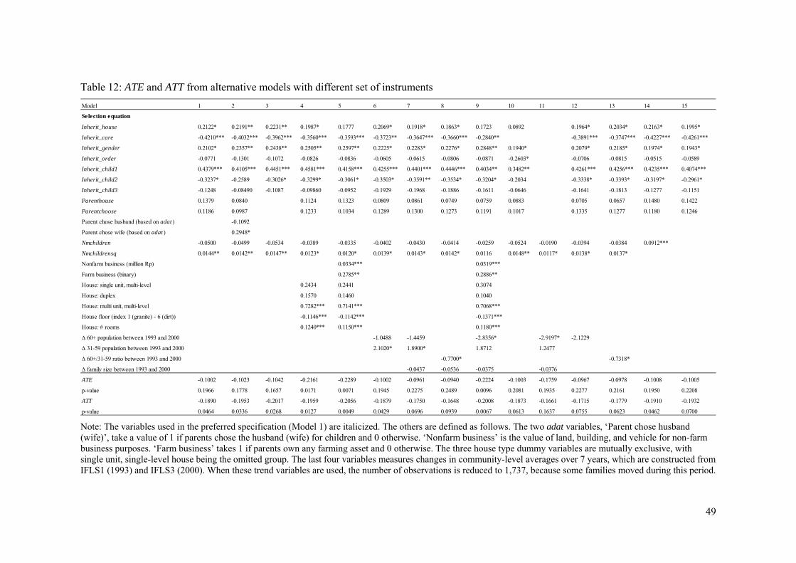
49
Table 12: ATE and ATT from alternative models with different set of instruments
Note: The variables used in the preferred specification (Model 1) are italicized. The others are defined as follows. The two adat variables, ‘Parent chose husband (wife)’, take a value of 1 if parents chose the husband (wife) for children and 0 otherwise. ‘Nonfarm business’ is the value of land, building, and vehicle for non-farm business purposes. ‘Farm business’ takes 1 if parents own any farming asset and 0 otherwise. The three house type dummy variables are mutually exclusive, with single unit, single-level house being the omitted group. The last four variables measures changes in community-level averages over 7 years, which are constructed from IFLS1 (1993) and IFLS3 (2000). When these trend variables are used, the number of observations is reduced to 1,737, because some families moved during this period.
Model 1 2 3 4 5 6 7 8 9 10 11 12 13 14 15
Selection equation
Inherit_house 0.2122* 0.2191** 0.2231** 0.1987* 0.1777 0.2069* 0.1918* 0.1863* 0.1723 0.0892 0.1964* 0.2034* 0.2163* 0.1995*
Inherit_care -0.4210*** -0.4032*** -0.3962*** -0.3560*** -0.3593*** -0.3723** -0.3647*** -0.3660*** -0.2840** -0.3891*** -0.3747*** -0.4227*** -0.4261***
Inherit_gender 0.2102* 0.2357** 0.2438** 0.2505** 0.2597** 0.2225* 0.2283* 0.2276* 0.2848** 0.1940* 0.2079* 0.2185* 0.1974* 0.1943*
Inherit_order -0.0771 -0.1301 -0.1072 -0.0826 -0.0836 -0.0605 -0.0615 -0.0806 -0.0871 -0.2603* -0.0706 -0.0815 -0.0515 -0.0589
Inherit_child1 0.4379*** 0.4105*** 0.4451*** 0.4581*** 0.4158*** 0.4255*** 0.4401*** 0.4446*** 0.4034** 0.3482** 0.4261*** 0.4256*** 0.4235*** 0.4074***
Inherit_child2 -0.3237* -0.2589 -0.3026* -0.3299* -0.3061* -0.3503* -0.3591** -0.3534* -0.3204* -0.2034 -0.3338* -0.3393* -0.3197* -0.2961*
Inherit_child3 -0.1248 -0.08490 -0.1087 -0.09860 -0.0952 -0.1929 -0.1968 -0.1886 -0.1611 -0.0646 -0.1641 -0.1813 -0.1277 -0.1151
Parenthouse 0.1379 0.0840 0.1124 0.1323 0.0809 0.0861 0.0749 0.0759 0.0883 0.0705 0.0657 0.1480 0.1422
Parentchoose 0.1186 0.0987 0.1233 0.1034 0.1289 0.1300 0.1273 0.1191 0.1017 0.1335 0.1277 0.1180 0.1246
Parent chose husband (based on adat ) -0.1092
Parent chose wife (based on adat ) 0.2948*
Nmchildren -0.0500 -0.0499 -0.0534 -0.0389 -0.0335 -0.0402 -0.0430 -0.0414 -0.0259 -0.0524 -0.0190 -0.0394 -0.0384 0.0912***
Nmchildrensq 0.0144** 0.0142** 0.0147** 0.0123* 0.0120* 0.0139* 0.0143* 0.0142* 0.0116 0.0148** 0.0117* 0.0138* 0.0137*
Nonfarm business (million Rp) 0.0334*** 0.0319***
Farm business (binary) 0.2785** 0.2886**
House: single unit, multi-level 0.2434 0.2441 0.3074
House: duplex 0.1570 0.1460 0.1040
House: multi unit, multi-level 0.7282*** 0.7141*** 0.7068***
House floor (index 1 (granite) - 6 (dirt)) -0.1146*** -0.1142*** -0.1371***
House: # rooms 0.1240*** 0.1150*** 0.1180***
∆ 60+ population between 1993 and 2000 -1.0488 -1.4459 -2.8356* -2.9197* -2.1229
∆ 31-59 population between 1993 and 2000 2.1020* 1.8900* 1.8712 1.2477
∆ 60+/31-59 ratio between 1993 and 2000 -0.7700* -0.7318*
∆ family size between 1993 and 2000 -0.0437 -0.0536 -0.0375 -0.0376
ATE -0.1002 -0.1023 -0.1042 -0.2161 -0.2289 -0.1002 -0.0961 -0.0940 -0.2224 -0.1003 -0.1759 -0.0967 -0.0978 -0.1008 -0.1005
p-value 0.1966 0.1778 0.1657 0.0171 0.0071 0.1945 0.2275 0.2489 0.0096 0.2081 0.1935 0.2277 0.2161 0.1950 0.2208
ATT -0.1890 -0.1953 -0.2017 -0.1959 -0.2056 -0.1879 -0.1750 -0.1648 -0.2008 -0.1873 -0.1661 -0.1715 -0.1779 -0.1910 -0.1932
p-value 0.0464 0.0336 0.0268 0.0127 0.0049 0.0429 0.0696 0.0939 0.0067 0.0613 0.1637 0.0755 0.0623 0.0462 0.0700

50
Figure 1. Baseline health, health outcomes, and coresidence status
Note: The vertical axis indicates the sample proportion for each health outcome. For example, 46 percent of coresiding parents who were unhealthy in the base year died within the next seven years.
0
10
20
30
40
50
0
10
20
30
40
50
DeathVery unhealthy
UnhealthyHealthy
Very healthy DeathVery unhealthy
UnhealthyHealthy
Very healthy
Baseline: Unhealthy Baseline: Healthy
Non coresidence Coresidence
%

51
Figure 2. Estimated Marginal Treatment Effect (MTE)
Note: The horizontal axis represents the value of DU , labelled by its cumulative probability. The vertical
axis measures the size of the MTE.
-0.8
-0.6
-0.4
-0.2
0
0.2
0.4
0.6
0.02 0.05 0.11 0.21 0.34 0.50 0.66 0.79 0.89 0.95 0.98
MTE - 2σ MTE MTE + 2σ

52
Appendix
ATE on survival from competing models
ATE Std. error (1) Unconditional mean differences a,e -0.0527 0.0236** (2) Linear probability model without selection on unobservables b,c,e -0.0364 0.0236 (3) Linear IV b,d,e -0.0854 0.1501 (4) Probit model without selection on unobservables c,e,f -0.0359 0.0240 (5) Probit model IV d,e,f -0.1041 0.2313 (6) Ordered model, constant effect, without selection on unobservables c,f,g -0.0481 0.0193** (7) Ordered model, heterogeneous effect, without selection on unobservables c,f,h -0.0391 0.0809 (8) Ordered model, heterogeneous effect, selection on unobservables (our preferred model) d,f
-0.1002 0.0775
Note:
a E Y1|D 1 E Y0|D 0 . b Linear probability model of Survive on Coresidence and other covariates with a common treatment assumption, Y Xβ γD U. c Coresidence is assumed to be exogenous. d Coresidence is assumed to be endogenous and estimation is with the instruments listed in Table 3. e The dependent variable Y 1 if a parent survives and 0 otherwise. f Maximum likelihood estimation with normally distributed unobservables. g A standard ordered probit model.
h Restriction of no selection on unobservables is imposed in the full model (8), e.g., α0 α1 0.