‘Urban Informal Sector and Poverty– Effects of Trade Reform in India’

Saibal KarCentre for Studies in Social Sciences, Calcutta, India

• Main Issues• First, how liberalization of trade and

investment, privatization and dismantling of the public sector has affected the present state of the informal sector in India.

• Second, what impact have such changes lain on the incidence of income poverty in India.

Scope and Contribution

• Aggregate level Study for 15 major states in India.• Regional Level Survey-Based Micro-study for the

province of West Bengal – Major Urban Areas.• The period under consideration is 1984-85 to

2000-01.• A detailed and systematic analysis of the effect of

trade related reforms on the existence of urban informal sector.

• Target variable is Incidence of Poverty, Depth of Poverty and Severity of Poverty as influenced by changes in conditions in the Urban Informal Sector.

Background Paper

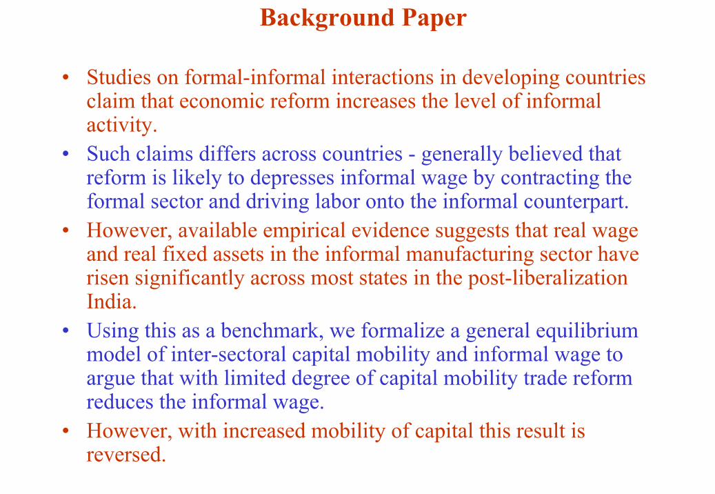
• Studies on formal-informal interactions in developing countries claim that economic reform increases the level of informal activity.

• Such claims differs across countries - generally believed that reform is likely to depresses informal wage by contracting the formal sector and driving labor onto the informal counterpart.

• However, available empirical evidence suggests that real wage and real fixed assets in the informal manufacturing sector have risen significantly across most states in the post-liberalization India.

• Using this as a benchmark, we formalize a general equilibrium model of inter-sectoral capital mobility and informal wage to argue that with limited degree of capital mobility trade reform reduces the informal wage.

• However, with increased mobility of capital this result is reversed.

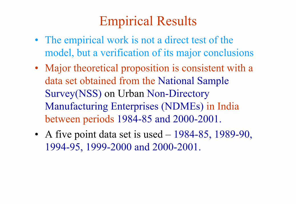
Empirical Results• The empirical work is not a direct test of the

model, but a verification of its major conclusions• Major theoretical proposition is consistent with a

data set obtained from the National Sample Survey(NSS) on Urban Non-Directory Manufacturing Enterprises (NDMEs) in India between periods 1984-85 and 2000-2001.

• A five point data set is used – 1984-85, 1989-90, 1994-95, 1999-2000 and 2000-2001.

Motivation and Perspective• Majority of the workforce in developing countries

(70 - 90%) are engaged in informal activities conducted in the so-called unorganized segment of the economy

• What is an Informal Sector?• Initially coined by ILO (1972) to mean “ illicit or illegal activities by individuals operating

outside formal sphere for the purpose of evading taxation or regulatory burden”

Alternatively, “ very small enterprises that use low-technology models and do not refer to legal status”. (Webster and Fidler, 1996).

In our case, informal sector -mix of these definitions and NDME’s employ less than 5 people.

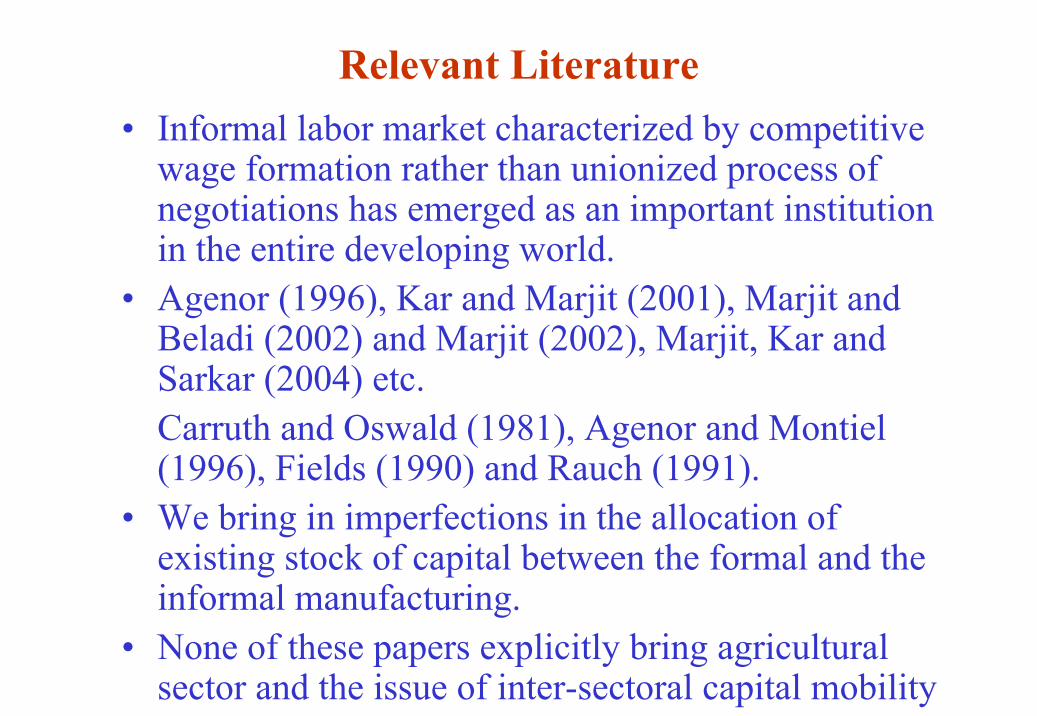
Relevant Literature• Informal labor market characterized by competitive

wage formation rather than unionized process of negotiations has emerged as an important institution in the entire developing world.

• Agenor (1996), Kar and Marjit (2001), Marjit andBeladi (2002) and Marjit (2002), Marjit, Kar and Sarkar (2004) etc.Carruth and Oswald (1981), Agenor and Montiel(1996), Fields (1990) and Rauch (1991).

• We bring in imperfections in the allocation of existing stock of capital between the formal and the informal manufacturing.

• None of these papers explicitly bring agricultural sector and the issue of inter-sectoral capital mobility

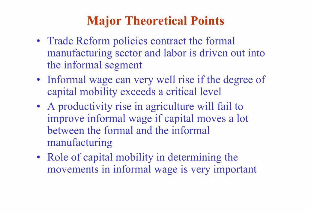
Major Theoretical Points• Trade Reform policies contract the formal

manufacturing sector and labor is driven out into the informal segment

• Informal wage can very well rise if the degree of capital mobility exceeds a critical level

• A productivity rise in agriculture will fail to improve informal wage if capital moves a lot between the formal and the informal manufacturing

• Role of capital mobility in determining the movements in informal wage is very important

Policy Implications• General Belief: (1)Downsizing protected

industries will drive labor to the informal segment with lower wage and poorer working conditions

• (2) Land reforms and other measures that enhance agricultural productivity are welcome since the informal sector is where most of the poor are located

• Note (2) is universally accepted both from a historical perspective as well as from the viewpoint of contemporary policy analyses

Caveat• Higher agricultural productivity must create an

excess demand for labor at the ongoing wage rate for the wage rate to improve

• If there is a strong link between the urban informal wage and the rural wage, there can be a reverse migration initially from the urban to the rural areas

• In case capital can quickly relocate itself within the urban sectors, the pressure on the informal, and subsequently, the rural wage would be considerably relaxed

• This implies, if capital is perfectly mobile between urban formal and informal sectors, land reform would not increase rural wage

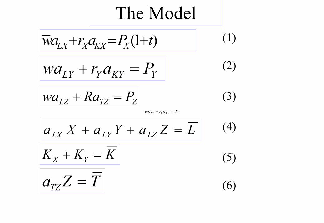
The Model

YKYYLY Parwa =+

(1)

(2)

(3)

(4)

(5)

(6)

)1( tParaw XKXXLX +=+

YKYYLY Parwa =+

ZTZLZ PRawa =+

LZaYaXa LZLYLX =++

KKK YX =+

TZaTZ =

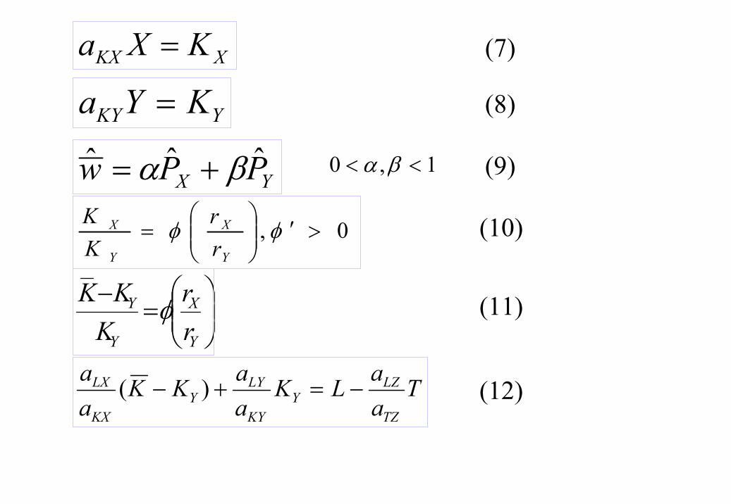
XKX KXa = (7)

YKY KYa = (8)

YX PPw ˆˆˆ βα += (9)1,0 << βα

0, >′

= φφ

Y

X

Y

X

rr

KK (10)

=

−

Y

X

Y

Y

rr

KKK φ (11)

TaaLK

aaKK

aa

TZ

LZY

KY

LYY

KX

LX −=+− )( (12)

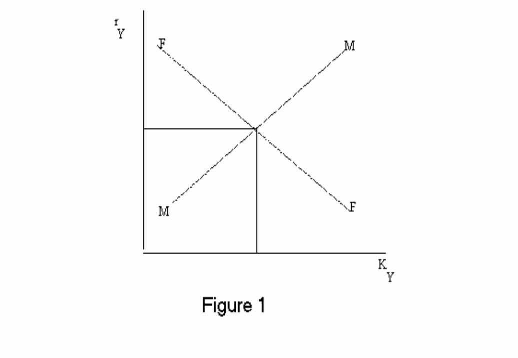
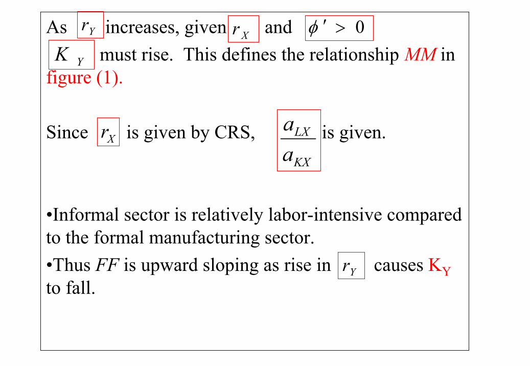
As increases, given and must rise. This defines the relationship MM in

figure (1).

Since is given by CRS, is given.

•Informal sector is relatively labor-intensive compared to the formal manufacturing sector.•Thus FF is upward sloping as rise in causes KYto fall.

0>′φ

YK

XrKX

LX

aa

YrXr

Yr

• We define as the elasticity of capital mobility between sectors X and Y.

• Depending on the elasticity of capital mobility between X and Y, we obtain the expression for changes in the informal wage.

φδδφε YX

YX

rrrr

/)/(

=

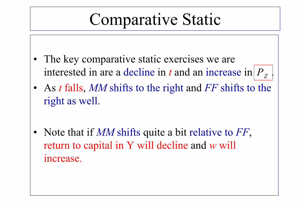
Comparative Static

• The key comparative static exercises we are interested in are a decline in t and an increase in .

• As t falls, MM shifts to the right and FF shifts to the right as well.

• Note that if MM shifts quite a bit relative to FF, return to capital in Y will decline and w will increase.

ZP

Impact on Informal Wage

• The precise condition for dw/dt > 0 is derived by following the above argument. There is an increase in the informal wage if the following condition is satisfied,

>>

KX

LXXX fKiffw

λλσε,,0ˆ

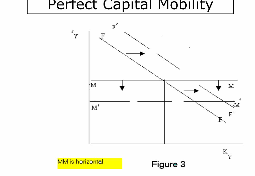
Perfect Capital Mobility

Empirical Results•Annual growth rates of real informal wage (IW), real fixed assets (FA) and real value added (VA) (in 1989

prices) for the informal sector as well as that of the real rural wage (RW) across different States and Union

Territories in India are tabulated. •1984-85 (NSS, 40th Round), 1989-90 (NSS, 45th

Round), 1994-95 (NSS, 50th Round), 1999-2000 (NSS, 55th Round) and 2000-2001 (NSS, 56th

Round).•Regressing Real IW on Real FA, VA and RW

(TABLE 1).

Annual Growth Rates of Informal Real Wage

-30

-20

-10

0

10

20

30

40

50

AP AS BH GJ HY HP KA KE MP MH OR PN RJ TN TR UPWB AN CH DN DH LA PO GO JK MA ME MINA SI

States

Perc

enta

ge

84-85 89-90 89-90 94-95 94-95 99-00 99-00 00-01 PostRefAvg

An n u al G ro w th Rate s o f F o rmal Re al Cap ita l Sto ck an d In fo rmal Re al F ixe d Asse ts

-30

-10

10

30

50

70

90

110

130

150

AP AS BH GJ HY HP KA KE MPMH OR PN RJ TN TR UPWB AN CH DN DH PO GO JK MA ME NA

State s

Perc

enta

ge

84-85 89-90(F ) 84-85 89-90(I) 89-90 94-95(F )89-90 94-95(I) 94-95 99-00(F ) 94-95 99-00(I)

Annual Growth Rates of Informal Real Fixed Assets

-50

0

50

100

150

200

AP AS BH GJHY HP KA KE MP MH OR PN RJ TN TR UPWB AN CH DN DH LA PO GO JK MA ME MINA SI

States

Perc

entg

e

84-85 89-90 89-90 94-95 94-95 99-00 99-00 00-01

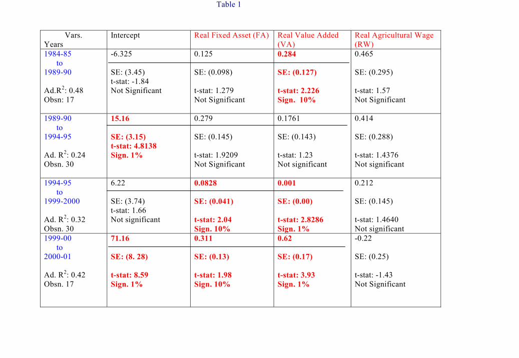
Table 1

Vars. Years

Intercept Real Fixed Asset (FA) Real Value Added (VA)

Real Agricultural Wage (RW)

1984-85 to 1989-90 Ad.R2: 0.48 Obsn: 17

-6.325 SE: (3.45) t-stat: -1.84 Not Significant

0.125 SE: (0.098) t-stat: 1.279 Not Significant

0.284 SE: (0.127) t-stat: 2.226 Sign. 10%

0.465 SE: (0.295) t-stat: 1.57 Not Significant

1989-90 to 1994-95 Ad. R2: 0.24 Obsn. 30

15.16 SE: (3.15) t-stat: 4.8138 Sign. 1%

0.279 SE: (0.145) t-stat: 1.9209 Not Significant

0.1761 SE: (0.143) t-stat: 1.23 Not significant

0.414 SE: (0.288) t-stat: 1.4376 Not significant

1994-95 to 1999-2000 Ad. R2: 0.32 Obsn. 30

6.22 SE: (3.74) t-stat: 1.66 Not significant

0.0828 SE: (0.041) t-stat: 2.04 Sign. 10%

0.001 SE: (0.00) t-stat: 2.8286 Sign. 1%

0.212 SE: (0.145) t-stat: 1.4640 Not significant

1999-00 to 2000-01 Ad. R2: 0.42 Obsn. 17

71.16 SE: (8. 28) t-stat: 8.59 Sign. 1%

0.311 SE: (0.13) t-stat: 1.98 Sign. 10%

0.62 SE: (0.17) t-stat: 3.93 Sign. 1%

-0.22 SE: (0.25) t-stat: -1.43 Not Significant

Table 2. Testing Structural Break at 1989-90Regressing IW on D1 (Intercept Dummy), FA, VA, RW between 1984-85

to 1989-90 and 1989-90 to 1999-00. (RSS1=22.597, Ad. R2 = 0.73).

Variables

Coefficient Standard Error t-stat Significance

Level

D1 0.0966 0.1488 0.6489 Not Significant

Fixed Asset

(FA)

0.3930 0.0685 5.7304 1%

Value Added

(VA)

0.0020 0.0006 3.2385 1%

Rural Wage

(RW)

0.8275 0.1668 4.9590 1%

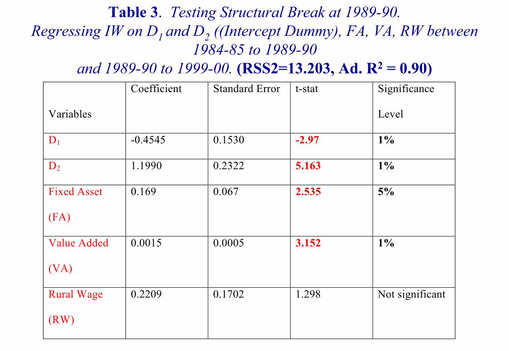
Table 3. Testing Structural Break at 1989-90.Regressing IW on D1 and D2 ((Intercept Dummy), FA, VA, RW between

1984-85 to 1989-90and 1989-90 to 1999-00. (RSS2=13.203, Ad. R2 = 0.90)

Variables

Coefficient Standard Error t-stat Significance

Level

D1 -0.4545 0.1530 -2.97 1%

D2 1.1990 0.2322 5.163 1%

Fixed Asset

(FA)

0.169 0.067 2.535 5%

Value Added

(VA)

0.0015 0.0005 3.152 1%

Rural Wage

(RW)

0.2209 0.1702 1.298 Not significant

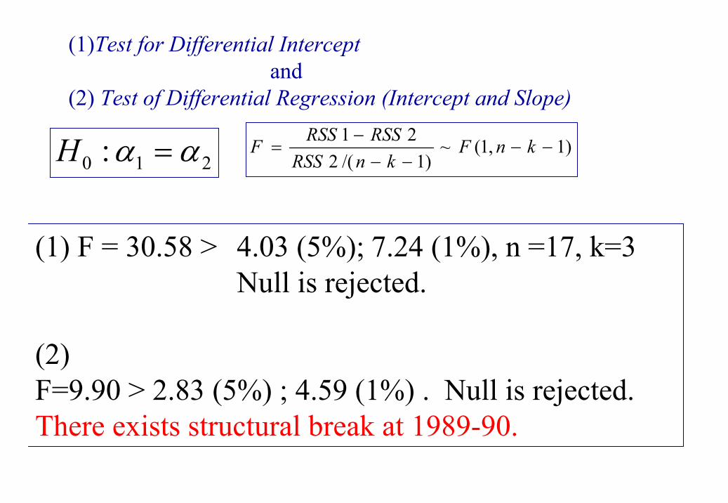
(1)Test for Differential Interceptand

(2) Test of Differential Regression (Intercept and Slope)

210 : αα =H )1,1(~)1/(2

21−−

−−−

= knFknRSS

RSSRSSF

(1) F = 30.58 > 4.03 (5%); 7.24 (1%), n =17, k=3Null is rejected.

(2)F=9.90 > 2.83 (5%) ; 4.59 (1%) . Null is rejected.There exists structural break at 1989-90.

Methodology for Proposed Research

• Most Important Section – Linking the results above to incidence, depth and severity of Poverty in Indian States

• A special case-study of the Province of West Bengal, where informal sector has contributed largely to employment growth.

• Proposed research links directly the changes in Informal Sector to the magnitude of Income Poverty.

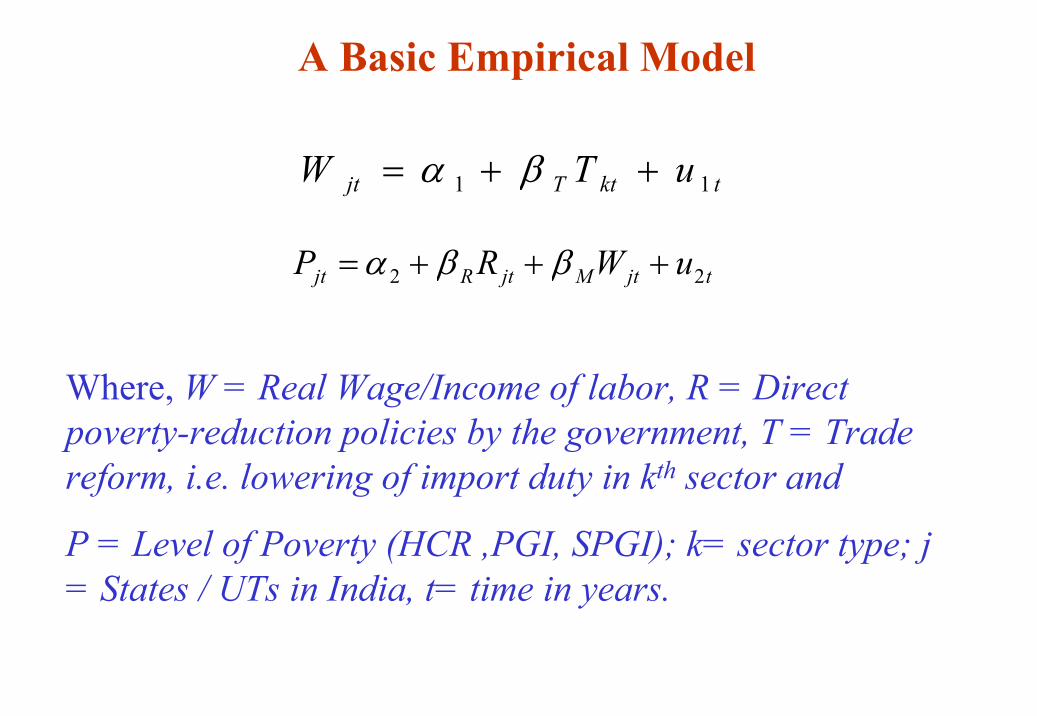
A Basic Empirical Model

tktTjt uTW 11 ++= βα

Where, W = Real Wage/Income of labor, R = Direct poverty-reduction policies by the government, T = Trade reform, i.e. lowering of import duty in kth sector and

P = Level of Poverty (HCR ,PGI, SPGI); k= sector type; j = States / UTs in India, t= time in years.

tjtMjtRjt uWRP 22 +++= ββα

Preliminary Results

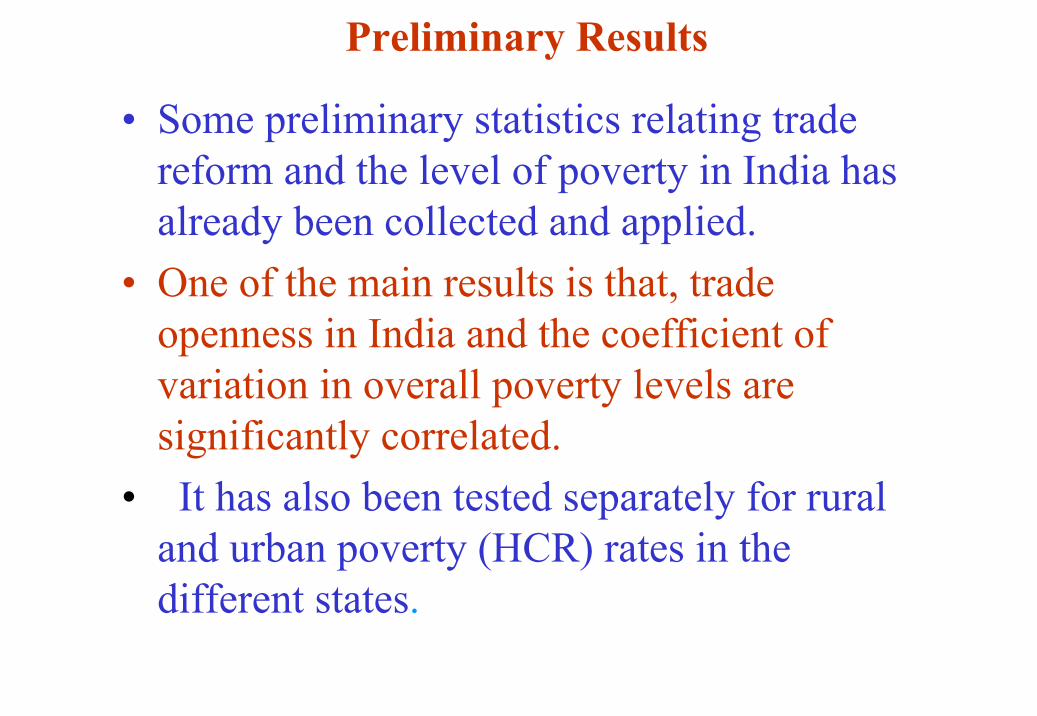
• Some preliminary statistics relating trade reform and the level of poverty in India has already been collected and applied.

• One of the main results is that, trade openness in India and the coefficient of variation in overall poverty levels are significantly correlated.

• It has also been tested separately for rural and urban poverty (HCR) rates in the different states.

State-wise Percentage of Population Below Poverty Line in India1973-74 1977-78 1983-84 1987-88 1993-94 1999-00

State / UT % % % % % %Andhra Pradesh 48.86 39.31 28.91 25.86 22.19 15.77Arunachal Pradesh 51.93 58.32 40.88 36.22 39.35 33.47Assam 51.21 57.15 40.77 36.21 40.86 36.09Bihar 61.91 61.55 62.22 52.13 54.96 42.6Goa 44.26 37.23 18.9 24.52 14.92 4.4Gujarat 48.15 41.23 32.79 31.54 24.21 14.07Haryana 35.36 29.55 21.37 16.64 25.05 8.74Himachal Pradesh 26.39 32.45 16.4 15.45 28.44 7.63Jammu and Kashmir 40.83 38.97 24.24 23.82 25.17 3.48Karnataka 54.47 48.78 38.24 37.53 33.16 20.04Kerala 58.79 52.22 40.42 31.79 25.43 12.72Madhya Pradesh 61.78 61.78 49.78 43.07 42.52 37.43Maharashtra 53.24 55.88 43.44 40.41 36.86 25.02Manipur 49.96 53.72 37.02 31.35 33.76 28.54Meghalaya 50.2 55.19 38.81 33.92 37.92 33.87Mizoram 50.32 54.38 36 27.52 25.66 19.47Nagaland 50.81 56.04 39.25 34.43 37.92 32.67Orissa 66.18 70.07 65.28 55.58 48.56 47.15Punjab 28.15 19.27 16.18 13.2 11.77 6.16Rajasthan 46.14 37.42 34.46 35.15 27.41 15.28Sikkam 50.86 55.89 39.71 36.06 41.43 36.55Tamil Nadu 54.94 54.79 51.66 43.39 35.03 21.12Tripura 51 56.88 40.03 35.23 39.01 34.44Uttar Pradesh 57.07 49.05 47.07 41.46 40.85 31.15West Bengal 63.43 60.52 54.85 44.72 35.66 27.02Andaman and Nicobar Islands 55.56 55.42 52.13 43.88 34.47 20.99Chandigarh 27.96 27.32 23.79 14.67 11.35 5.75Dadra and Nagar Haveli 46.55 37.2 15.67 67.11 50.84 17.14Delhi 49.61 33.23 26.22 12.41 14.69 8.23Daman and Diu - - - - 15.8 4.44Lakshadweep 59.68 52.79 42.36 34.95 25.04 15.6Pondicherry 53.82 53.25 50.05 41.46 37.4 21.67All-India 54.88 51.32 44.48 38.86 35.97 26.1Mean 49.9812903 48.285484 37.706452 34.247742 31.802813 21.521875SD 9.89189862 12.069334 13.145667 12.506225 11.184037 12.388167COV 19.791203 24.995782 34.863177 36.516934 35.166816 57.560819

Source: NSSO - various rounds and own calculations

Y ear TO I C O V 1973-74 8 .825059 19 .7912

1977-78 12 .58812 24 .99578

1983-84 12 .6399 34 .86318

1987-88 11 .99442 36 .51693

1993-94 18 .32613 35 .16682

1999-00 21 .21388 57 .56082

S ource: Foreign T rade S tatistics of Ind ia, N SS O and ow n calcu lations

Figu re 1

Trends in Trade O penness and C oefficient of V ariation in Poverty

0

10

20

30

40

50

60

70

1973-74 1977-78 1983-84 1987-88 1993-94 1999-00Years

Degrees

Trade O peness CO V of Poverty across States

References

• Agenor, P, 1996, The labor market and economic adjustment, IMF Staff Papers 32, 261-335. • Agenor, P & P. Montiel, 1996, Development Macroeconomics, Princeton, NJ: Princeton University

Press• Banerjee, A, P. Gertler & M. Ghatak, 2002, Empowerment and efficiency: The economics of a

tenancy reform, Journal of Political Economy, 110, 2, 239-80.• Carruth, A & A. Oswald, 1981, The determination of union and non-union wage rates, European

Economic Review 16, 2/3, 285-302.• De Soto, Hernando, 2000, The Mystery of Capital, USA: Basic Books.• Fields, G, 1990, Labour market modelling and the urban informal sector: Theory and evidence, in:

D. Turnham, eds, The informal sector and evidence revisited, (OECD, Paris)• Jones, R.W & Marjit, S, 1992, International trade and endogenous production structure; In, W.

Neuefeind, & R. Reizman (Eds.), Economic Theory and International Trade- Essays in Honor of J. Trout Rader. Springer.

• Kar, S & Sugata Marjit, 2001, Informal sector in general equilibrium: welfare effects of trade policy reforms, International Review of Economics and Finance 10, 289-300.

• Marjit, Sugata, 1991, Agro-based industry and rural-urban migration: A case for an urban employment subsidy, Journal of Development Economics, 35,2, 393-98.

• Marjit, Sugata, 2003, Economic reform and informal wage- A general equilibrium analysis, Journal of Development Economics, September.

• Marjit, S & R. Acharyya, 2003, International Trade, Wage Inequality and the Developing Economy – A General Equilibrium Approach, Heidelberg and NY: Physica- Verlag.

• Marjit, S & H. Beladi, 2002, The Stolper-Samuelson theorem in a wage differential framework, The Japanese Economic Review 53, 2, 177-181.

• National Sample Survey, 1985 (40th Round), 1989 (45th Round), 1995 (50th Round), Survey of unorganized manufacture, Department of Statistics, Government of India.

• Rauch, James, 1991, Modeling the informal sector formally, Journal of Development Economics