AUGMENTING THE OPERATIONAL ... - Xylem Global Brands
34
AUGMENTING THE OPERATIONAL CAPABILITIES OF SONTEK/YSI STREAMFLOW MEASUREMENT PROBES Objectives #1 & #2: On the performance of index-velocity to deliver accurate streamflows and support flood warnings: Case studies featuring SonTek/YSI-SL capabilities Submitted to: SonTek/YSI Incorporated 9940 Summers Ridge Road San Diego, CA 92121 Submitted by: Marian Muste (Principal Investigator) Research Engineer (IIHR-Hydroscience & Engineering) Adjunct Professor, Civil & Environmental Engineering Department The University of Iowa, Iowa City, IA, U.S.A. Email: [email protected]; Phone: 319 384 0624 Dongsu Kim Associate Professor Civil & Environmental Engineering Dankook University, Yongin, Gyeonggi, South Korea Iowa City, April 24, 2020
Transcript of AUGMENTING THE OPERATIONAL ... - Xylem Global Brands

AUGMENTING THE OPERATIONAL CAPABILITIES OF SONTEK/YSI STREAMFLOW MEASUREMENT PROBES
Objectives #1 & #2: On the performance of index-velocity to deliver accurate streamflows and support flood warnings:
Case studies featuring SonTek/YSI-SL capabilities
Submitted to: SonTek/YSI Incorporated 9940 Summers Ridge Road
San Diego, CA 92121
Submitted by: Marian Muste (Principal Investigator)
Research Engineer (IIHR-Hydroscience & Engineering) Adjunct Professor, Civil & Environmental Engineering Department
The University of Iowa, Iowa City, IA, U.S.A. Email: [email protected]; Phone: 319 384 0624
Dongsu Kim
Associate Professor Civil & Environmental Engineering
Dankook University, Yongin, Gyeonggi, South Korea
Iowa City, April 24, 2020

SonTek/YSI – IIHR Collaborative Research Report
2
EXECUTIVE SUMMARY
The most reliable method to measure streamflows in natural streams is the direct acquisition of
discharge measurements. These measurements requires deployment of instruments and personal in the field and, in some cases, traversing the stream with measurement equipment several times. The most efficient contemporary instrument for direct discharge measurements is the Acoustic Doppler Current Profilers (ADCPs) which measure flows relatively fast and accurate (±5.4 - 7.4 % in steady flows according to Boldt & Oberg, 2015). During high flows, however, direct measurements are challenging because the adversity of the flow environment for the operators and equipment (WMO, 2010). While there are intensive efforts to conduct unassisted direct discharge measurement, currently only indirect approaches are used for continuous monitoring at station located in streams or rivers (Dottori et al., 2009). Specifically, real-time monitoring is based on the conventional stage-discharge method (labeled herein as HQRC) and, increasingly, on the index-velocity method (labelled herein as IVRC).
Conventional monitoring methods rely on relationships (a.k.a., ratings) that link direct streamflow measurements with real-time, continuous measurements of independent variables that are easier captured with instruments deployed permanently at the site (e.g., stage or velocity). The simultaneous measurements for rating development are acquired episodically with the goal to cover the whole flow range passing through the monitoring site. The such-obtained ratings are essentially one-to-one relationships that are used to monitor both steady and unsteady flows despite that for the latter flow conditions the ratings do not properly account for the hysteretic behavior of the flow variables (Muste & Hoitink, 2017). Hysteresis, a key concept for the present study, is a generic term indicating that the status of a system at any given point is dependent on its history to reach that state (i.e., the state depends on the process memory). Such a process occurs when the gradual propagation of a natural flood wave enters the stream due to runoff produced in the station’s drainage area by rainfalls.
It is important to mention upfront that unsteady flows are ephemeral and, in many situations, their effects on the conventional methods are small, therefore no action is required. This is certainly the case for flows propagating as kinematic waves on larger streambed slopes. However, for intermediate and lowland streams exposed to fast-varying flows the hysteresis becomes prominent. While hysteresis is a process known to monitoring agencies, it has only received attention in flood-prone areas of large rivers (e.g., Mississippi) with the purpose to provide more accurate data for the streamflow forecasting models (Holmes, 2016) and more recently in areas subjected to highly unsteady flows (Morlock et al., 2002). In many other medium and small inland rivers (i.e., non-tidal) hysteresis is not accounted for, as there is a perception in the hydrometry community that the hysteresis effect is small and cannot be discerned from the uncertainty of the instruments (Holmes, 2016). The same study found that out of 5,420 USGS gaging sites that use stage-discharge ratings, 67% of the stations are potentially moderately or strongly affected by hysteresis. Currently, there is no systematic effort to evaluate the impact of hysteresis in medium and smaller streams despite that such streams experience more frequent and intense events that favors development of hysteresis (e.g., Messner & Meyer, 2006; Mallakpour & Villarini, 2015).
The most promising approach for continuous monitoring streamflows in hysteresis-prone areas is the index-velocity method. Currently, USGS operates and maintains approximately 500 index-velocity stations and the use of this method is expected to grow. Many of these gaging stations are equipped with the SonTek/YSI HADCP, dubbed by the manufacturer as the Side-Looker (SonTek-SL). In contrast to the stage-discharge method, which fails to capture the dynamics of the flood wave propagation, the index-velocity method can directly measure hysteresis in real time by combining the index-velocity (a direct indication of the flow dynamics) and stage (purely geometric descriptor of the flow) measurements. As a

SonTek/YSI – IIHR Collaborative Research Report
3
result, the IVRC discharge estimates are closer to the actual flows. While reducing substantially the uncertainty associated with the estimation of discharges during unsteady flows compared to the stage-discharge method, The IVRC method can be itself affected by hysteresis. As of today, there are no comprehensive studies or experimental evidence to document the performance of the IVRC method in steady and unsteady flows.
The motivation for this study stems in the authors’ perception that there is a sensible gap between the available analytical knowledge on river mechanics and the fundamental principles employed by the monitoring methods as well as on the capabilities of the new generation of high-resolution instruments, such as SonTek-SLs, to accurately measure streamflows unsteady flows. Of special focus in this study is the assessment of the IVRC capability to measure streamflows during floods when the accuracy and timeliness of the data are needed most. Furthermore, we realize that the IVRC method has not been used at its full potential as this method is also able to distinguish the separation of hydrographs for the directly measured variables (i.e., velocity and stage) in unsteady flows. The latter capability opens possibility to use IVRC monitoring methods for forecasting purposes without involving any modeling.
The present research builds upon the theory of unsteady flow in open channels, fundamentals of the index-velocity method, and SonTek-SL datasets available at USGS gaging stations to:
a) provide scientifically-sound methods to diagnose hysteresis at gaging sites and estimate severity of impacts on discharge measurements made with traditional stage-discharge ratings,
b) demonstrate the superiority of the index-velocity method to capture the characteristics of the flood wave propagation in natural streams prone to hysteresis
c) evaluate how monitoring data collected for the index-velocity method may be used to forecast flood crest magnitude and arrival time without involving any type of modeling.
To the knowledge of the present authors, the analysis approach and experimental evidence illustrated in this study have no precedent in hydrometric literature published so far. This observation is noteworthy as the analyzed case studies are solely based on publicly-available data collected with SonTek-SL at two exiting gaging stations: USGS station #05558300 and # 05568500. Extension of such analyses to a variety of sites can provide important insights in the flow processes associated with unsteady flows, their relationship to site characteristics as well on the practical information needed to the refine the IVRC methodology to monitor unsteady flows using the current or alternative protocols. The present analysis and additional insights from previous studies suggest that new protocols for IVRC ratings might be needed.
We expect that the outcomes of this IIHR-SonTek/YSI collaborative research will advance the IVRC method by both improving its accuracy for streamflow estimation in unsteady flows as well as expanding the IVRC-based gaging stations with forecasting functionality using the existing infrastructure and instruments. The main beneficiaries of this research are streamflow monitoring agencies, researchers and consultants using simulations of hydraulic routing of unsteady flows by providing additional datasets for model calibration/validation and enabling the assimilation of data into streamflow forecasting models. Furthermore, the project outcomes can better support managers charged with flood preparedness and informing the general public in flood-prone areas where flood forecasts are not currently available. It is expected that the broader community including planners, designers and operators of water resources projects will be also positively impacted by this research. The improved quality of the IVRC-based datasets can also support academic researchers in natural sciences who are conducting studies at field scales, an area of research becoming increasingly popular with the fast-paced development of new field equipment and remote sensing instruments.

SonTek/YSI – IIHR Collaborative Research Report
4
Table of Contents
Section Page Number
Executive Summary .....................................................................................................................2 1. Introduction ...................................................................................................................... 5 2. Review of relevant aspects for flows propagating at gaging stations ............................... 6
2.1 Flow regimes .............................................................................................................. 6 2.2 Hysteresis diagnostic formulas .................................................................................. 9
3. Principles, practice, and uncertainties in the index-velocity method (IVRC) estimates 12 3.1 Basic aspects ............................................................................................................. 12 3.2 Uncertainty considerations........................................................................................ 13
4. Analysis of IVRC use cases with SonTek-SL velocimeteres ........................................... 14 4.1. Analysis sites, terminology, and study approach ..................................................... 14 4.2. IVRC performance in steady flows.......................................................................... 16
4.3. IVRC performance during flood wave propagation ................................................. 17 4.4. Additional IVRC capabilities: flood crest forecasting ............................................. 25
5. Research finding summary & Future work ...................................................................... 26 6. Conclusion ........................................................................................................................ 30 7. References ......................................................................................................................... 31

SonTek/YSI – IIHR Collaborative Research Report
5
1. Introduction Recent advances in acoustic methods applied to river instrumentation are revolutionizing our
capabilities to understand, describe and model river systems. Especially useful are the acoustic-doppler velocimeters (ADP) that can quickly and efficiently provide detailed multi-dimensional velocity measurements that uniquely enable investigation of complex river processes that are related to critical riverine issues such as flooding, sediment transport, habitat availability and stream ecology. There is vast literature describing the underlying principles and the configurations of the acoustic-doppler velocimeters used to quantify stream hydrodynamics that usefully guide the selection and use of these instruments for various practical purposes (e.g., SonTek, 2000; www.sontek.com/media/pdfs/sontek-sl-white-paper.pdf). While the basic principles of operation for the acoustic technology remain largely unchanged since their adoption in riverine environments in early 1980’s, there are multiple attempts in the user communities to fully assess their operation performance in various flow conditions and to explore new capabilities for providing additional information from the extensive datasets they produce. The primary use of acoustic-doppler velocimeters has been, and still is, to obtain direct discharge estimates by efficiently profiling river cross sections. These direct measurements are widely used to construct relationships for continuous monitoring stations equipped with the stage-discharge method (Rantz et al., 1982; Kennedy, 1984). Acoustic-doppler velocimeters can be alternatively set at fixed locations to measure velocity profiles across the streams and rivers (vertical or side orientation) that combined with stage measurements provide discharge estimates via the index-velocity method (Morlock et al., 2002; Levesque & Oberg, 2012).
Currently, the U.S. Geological Survey (USGS) delivers real-time data for more than 8,500 sites across the nation (Eberts, et al., 2019). A recent evaluation of 5,420 USGS gaging sites using the stage-discharge ratings has found that 67% of them are moderately or strongly affected by hysteresis (personal communication from B, Holmes, USGS). The hydrometric community identifies hysteresis by the presence of distinct relationships between flow variables for the rising and falling stages of flood waves propagating through gaging stations. Most often, hysteresis is associated with “loops” in the stage-discharge relationships widely used for discharge estimation. However, hysteresis is a process linked to the flow propagation, therefore it is expected that it affects all the monitoring methods. The aforementioned finding on the bias in the stage-discharge estimates does not come as surprise, as it is well known that the use of the simple, one-to-one, stage-discharge relationship completely misses hysteresis produced by the propagation of unsteady flows (Rantz et al., 1982; Muste et al., 2020). The deviations of the actual flows from those estimated by stage discharge relationship can be considerable. For example, Faye & Cherry (1980), Di Baldassarre & Montanari (2009), and Herschy (2009) report discharge differences for the same stage from 9.8% to 34% in large rivers. Differences up to 40% were found between discharge estimates and direct ADCP measurements in a medium-size, low bed-slope river (Muste & Lee, 2013). While hysteresis is a process known to monitoring agencies, it has only received attention in major flood-prone areas along large rivers (e.g., Mississippi) with the purpose to provide more accurate data for streamflow forecasting models (Holmes, 2016). For these locations, purely empirical or semi-empirical approaches requiring additional measurements during events are applied to correct the stage-discharge ratings (Schmidt, 2002; and Dottori et al., 2009). Hysteresis occurring in medium and small inland rivers is, in most cases, undocumented as there is a perception in the hydrometry community that hysteresis impact is small and cannot be discerned from instrument uncertainty (Holmes, 2016).
Out of the total number of USGS operational gages, there are 500 stations that are using the index-velocity method for estimation of discharges. The index-velocity method works well in steady flows (e.g., Cheng et al., 2019) but it is especially recommended for measurements in areas where unsteady flow and backwater occur (e.g., Morlock et al., 2002). The hydrometric community makes continuous efforts to improve the index-velocity method (e.g., Le Coz et al., 2008, Nihei & Kimizu, 2008; and, Kastner et al., 2018, Cheng et al., 2019). However, at this time, the method performance has been much less investigated in comparison with the century-old stage-discharge approach. The use of index-velocity method is expected to grow, especially for hysteresis-prone areas, as discharge estimates can be produced at fast rates (of the

SonTek/YSI – IIHR Collaborative Research Report
6
order of minutes) bringing this method much closer to the performance of direct discharge measurements, the most reliable method to capture hysteresis in natural streams irrespective of the flow situation.
The available hydrometric literature does not offer criteria for comprehensive evaluation of the performance of the methods at hysteresis-prone sites nor for detecting the departure of the actual flows from the estimates provided by the conventional monitoring methods. There is no indication of systematic efforts for correcting or directly capturing hysteresis in the routine usage of the conventional monitoring methods. While the monitoring methods have improved over time through ingestion of new, superior instruments, the underlying protocols and associated assumptions have not been recently reviewed with respect to their capability for capturing hysteresis. Consequently, the ratings associated with stage-discharge and index-velocity methods continue to be constructed assuming essentially one-to-one relationships between flow variables without specifically distinguishing between flow phases.
Many of the nationwide index-velocity stations are equipped with SonTek/YSI Horizontal Acoustic Doppler Current Profilers (HADCP). The SonTek/YSI HADCP, dubbed by the manufacturer as the Side-Looker (SonTek-SL), is at the core of the index-velocity method by simultaneously and continuously measuring stage and velocities with probes collocated in the same unit (https://www.sontek.com/sontek-sl-series). The unit is specifically designed for side mounting on bridges, canal walls, or riverbanks, using a low-profile housing that makes installation easy. Since the initial stages of the SonTek-SL development, there has been a continuous dialogue between manufacturers and users on how better can the instrument fit its purpose. This dialogue has been meshed with evaluations and research activities that preceded the addition of new instrument hardware or software capabilities. The present study pertains to this category of exploratory studies. Given that the SonTek-SL is specifically designed to support the existing index-velocity method for continuous streamflow monitoring, this research will investigate the method’s performance and capabilities to estimate and predict flow variables in various flow conditions.
The present paper is organized as follows. First, the fundamentals of open channel flow theory, the principles of the index-velocity monitoring protocols, and the needed capabilities of the technology that underpin the method will be revisited. Following these reviews, recommendations on what additional developments are needed for advanced instruments such as SonTek-SL to better serve their purpose will be formulated. Emphasis will be placed on illustrating the superiority of the index-velocity over the stage-discharge method for capturing unsteady flows and the means of using direct SonTek-SL measured data to forecast flood warning without using additional modeling tools. Illustrations presented below are using data from Illinois USGS gaging stations #05558300 and # 05568500 both equipped with SonTek-SL probes.
2 Review of relevant aspects for flows propagating at gaging stations 2.1 Flow regimes
Gaging stations are placed in stream reaches carefully selected with consideration of the best practice guidelines (Rantz., et al. 1982). These criteria aim at reducing at the maximum possible the flow complexities within the stream reach and maintain a quasi-uniform flow distribution in the station vicinity. In other words, the monitoring site has to be set in a channel free of obstructions that maintains a quasi-uniform geometry in the streamwise direction, lacks considerable bed irregularities, and preserves the cross-sectional flow distribution for the whole range of flows at the station (Rantz et al., 1982). The latter condition is critically important for the index-velocity method for which velocities are measured along a fixed line across the stream. The deployment of the instruments and construction of the ratings are guided by analytical considerations that reflect flow conditions at the site and with detailed considerations of the instrument configuration and operational characteristics (Kennedy, 1984; and Levesque & Oberg, 2012).
The streamflows passing through a gaging station are commensurate with the meteorological conditions and/or human-controlled flow releases in the upstream drainage area or as point sources along the stream. The analytical description of these different type of flows is important for hydrometric purposes as it illustrates the data needs to attain a good tracing of the flows passing through the station. Provided below for completeness are some basic theoretical considerations as synthesized by the paper of Muste et al. (2020). The simplest flow situation that can occur within the reach adjacent to a monitoring station is the

SonTek/YSI – IIHR Collaborative Research Report
7
uniform and steady flow. In such a flow, the gravitational force driving the water movement in the streamwise direction is balanced by the friction force applied on the wetted area of the channel perimeter. Under these conditions, the Manning equation applies (Henderson, 1996): 2/3
0 01
sQ AR S K Sn
= =
(1)
where Qs is the flow discharge, n is Manning’s roughness coefficient, A is cross-sectional area, R is hydraulic radius, S0 is the slope of the bed, that in steady uniform flows is parallel to the energy slope, Se, and K = (1/n) AR2/3 is the channel conveyance (in metric units). To attain uniform flow, the channel cross section should maintain its shape (i.e., A, R, and h - the flow depth, remain constant throughout the reach) and have a straight alignment in the streamwise direction (i.e., no channel sinuosity). Note: the flow depth, h, is derived from stage, H, in hydrometric applications, therefore their use in the present context is interchangeable. The steady-uniform flow, the energy slope, Se, is equal to the free-surface slope, Sw, and streambed slope, S0, as shown in Figure 1a (left side). Equation (1) guides the construction of the stage-discharge ratings for all ranges of in-bank flows, excepting the very low flows. Typically, the stage-discharge rating is assumed as one-to-one relationship, as illustrated in Figure 1a (center). Using this unique relationship in the streamflow monitoring leads to a simultaneous occurrence of the Umax, Qmax and hmax as shown in the same Figure 1 (right).
During the annual seasonal cycle, the typically longer periods of steady-uniform flow regimes in the channel are interrupted by storm events or other flow contributions occurring upstream the gaging station. These flow perturbations creatie unsteady flows that propagate through a channel as gradually-varied waves (a.k.a. flood waves). During the flow transitions, Equation (1) is not strictly valid as the occurrence of unsteady flow (variation in time) is inherently associated with flow non-uniformity (variation in space). Illustration of the departure of the energy, water surface and bed slopes from the steady flow condition is provided in in Figure 1b (left). The most-often used analytical formulation for describing unsteady flows are the one-dimensional Saint-Venant equations derived from mass and momentum conservation laws applied to shallow-water flows (Saint-Venant, 1871; and Chow, 1959). In essence these equations prescribe the balance between the gravity, friction, pressure, and inertial forces applied to the body of moving water under the following assumptions: the flow is one-dimensional, fluid is incompressible, channel bed is relatively small, hydrostatic pressure distribution applies, vertical acceleration is negligible, and the friction losses are related to flow variables using relationship for steady flows. It is important to mention that these conditions are essentially met if the best practice guidelines for site selection are applied (i.e., quasi-prismatic and straight channels without lateral inflows or outflows). The Saint-Venant equations can take a variety of forms. For the present context, where we substantiate the departure of the unsteady flow from steady flow condition, the most useful relationship is the arrangement provided by Knight (2006) that relates the discharge in unsteady flow, Q, with the steady discharge, Qs, defined by Equation (1):
0 0 0
1 11s
kinematic wave
diffusion wave
full dynamic wave
h U U UQ QS x gS x gS t
∂ ∂ ∂= − − −
∂ ∂ ∂
→
→→→→
→→→→→→→→→→→→
(2)
where U is the cross section mean velocity, t is time, and x is the distance along the channel. Equation (2) is strictly valid for straight prismatic channels as it neglects the changes in momentum that occur from causes other than unsteadiness of flow non-uniformity. Comparison of Equations (1) and (2) shows that terms other than S0 may modify the character of the wave (Henderson, 1996).

SonTek/YSI – IIHR Collaborative Research Report
8
Figure 1 Illustration of the hysteretic effect on the stage-discharge relationship: (a) streamwise gradients
for energy and free-surface lines for steady uniform flows (left); stage-discharge ratings obtained with the one-to-one relationship (center), and, resultant hydrographs (right); (b) streamwise gradients for energy and free surface lines for unsteady flows (left); non-unique stage-discharge relationship (center), and,
non-overlapping hydrographs (right). Notations are as provided in Equations (1) and (2). Equation (2) provides a realistic hydraulic description of flood waves (i.e., non-uniform, unsteady
flows) irrespective of their type: kinematic (first term only), diffusion (first and second terms), and full dynamic (all terms). The distinction between the types of waves is based on the relative importance of the terms in Equation (2); i.e., when a term is an order of magnitude smaller than the others, it is considered practical to discard that term (Hunt, 1977). Equation (2) is strictly valid only for stages up to bankfull stage (a.k.a. as flood stage), as the mass and momentum exchanges that occur between the main channel and floodplain above this stage generate additional flow complexities not captured in the equation. There are other factors that can increase the flow complexity (e.g., instream vegetation, bedform-induced roughness, baseflow-stream interaction as well as issues related to synchronization of the instrumentations) and they can limit the use of Equation (2) in practical situations. The equation does not account for backwater effects, despite that in many practical situations unsteady flow and backwater are simultaneously involved.
The magnitude of the individual terms in Equation (2) is commensurate with the slope of the bed at the site and the intensity of the propagating wave (i.e., its magnitude vs. duration). During events the magnitude of the terms vary continuously commensurate with the degree of dispersion and subsistence of the propagating waves (Henderson, 1966; Ferrick, 1985). There are many investigations discussing wave types and their characteristics as, for example, Henderson (1966), Ponce & Simon (1977), Ferrick (1985), Fread (1985), Yen & Tsai (2001), Perumal et al. (2004), Moramarco et al. (2008a), and Dottori et al. (2009). Some of these investigations provide practical guidelines regarding the identification of the type of waves that can occur for specific sites and events. For example, Julien (2002), Shen & Diplas (2010), and Gosh (2014), recommend to apply the full dynamic wave (i.e., all terms in Equation 2) for inland rivers located on mild and small bed slopes. For large bed slopes, Arico (2009) recommends use of the kinematic wave (first term in Equation 2). Mrokowska et al. (2015) points out that paradoxically, the kinematic wave approximation is widely applied in cases for non-kinematic waves despite their significant differences.
The interplay among the terms in Equation (2) leads to non-unique relationships among the mean flow variables that are distinct for the rising and falling limb of the same wave propagating event, as illustrated in Figure 1b (center) for the relationship between stage and discharge. The departure of the unsteady limbs from the one-to-one relationships produced by hysteresis is generically labeled as a “loop” (Henderson 1966). Indicated on the loop are specific points related to the flow variable hydrographs discussed below. Another direct manifestation of the hysteresis presence is the pashing between the time series of the mean

SonTek/YSI – IIHR Collaborative Research Report
9
flow variables and their maximum values (a.k.a. peaks) as observed by Prowse (1984) in other areas of sciences. Figure 1b (right) illustrates that the peaks for the flow variables in unsteady flow do not occur simultaneously rather they are phased in time in the following order: energy slope, velocity, discharge and flow depth (stage). The discussion of the phasing of the mean flow variables has been central only for a handful of previous investigations that demonstrated analytically (e.g., Moots, 1927, Li et al., 2013) and experimentally (e.g., Graf & Song, 1996; Hunt, 1997; Nezu & Nakagawa, 1994; Nezu et al., 1997) that the arrival of the peaks for the flow variables of non-kinematic waves occurs in the following sequence: mean velocity followed by discharge and then by stage. The peak phasing is commensurate with the magnitude of hysteresis that in turn is directly dependent on the site conditions and wave dynamic characteristics. A special case of Equation (2) is the kinematic wave that does not develop considerable hysteretic loop nor display peak phasing being equivalent from this perspective to the steady flow situation (e.g., Lamberti & Pilati, 1990). This similarity is explained by the fact that kinematic wave occurs typically on large slopes where the gravity force largely exceeds both the inertia and pressure gradient forces hence the Equation (2) trims down to Equation (1) for steady flows.
The most compelling study on the peak variable phasing provided by Graf & Qu (2004) demonstrates analytically (using the Saint-Venant equations) and with laboratory experiments that the energy slope precedes the velocity-discharge-depth peak sequencing, as illustrated in Figure 2 (right). This pattern is expected as the creation of a wave needs first a pulse of energy that is subsequently transmitted into the water body through interconnected mean and turbulence internal transport mechanisms. The full spectrum of variable peak phase sequencing has been only recently captured in field conditions as the technical arrangement needed to measure continuously multiple flow variables is still challenging. One of such recent studies was conducted by Rowinski et al. (2000) using customized deployments with multiple instruments and measurement protocols. This arrangement allowed to capture time-varying free-surface and mean-velocity data that subsequently allowed to calculate real time free-surface and energy slopes during unsteady flows. Rowinski et al. found differences of about 30 mins between the free-surface slope and stage peaks for a small inland stream. For large rivers, this lag can be considerably increased as will be illustrated in Section 4 where differences between the maximum velocity (the second peak in the sequence) and maximum stage is of the order of days (1 to 3.5 days). These recent experiments illustrate that the advancements of the instruments make increasingly possible to acquire detailed measurements that can shed new insights into the hysteretic behavior of unsteady flows.
2.2 Hysteresis diagnostic formulas The most substantial inferences from the review on the open-channel regimes is that unsteady flows
generate a hysteretic behavior that further produce a non-unique relationship between any two of the flow variables and an out-of-phase timing of the flow hydrographs during the flood wave propagation. The hysteretic behavior is rooted in differences between the rising and falling stages of the unsteady flows that impact not the mean flow characteristics but also the distribution of turbulence (Bareš, Jirák, & Pollert, 2008; Hunt, 1997; Nezu & Nakagawa, 1995; S. Q. Yang & Chow, 2008). The severity of the hysteretic behavior is determined by the magnitudes of individual terms in Equation (2) that in turn are directly related to the slope of channel bed at the monitoring site and the intensity of the propagating wave. In other words, the type of wave resulting from a rainfall within the station’s drainage area depends of the gage-site location and event characteristics, i.e., the hysteretic behavior is site- and event-specific. The subsequent discussions describes means to detect both the potential of hysteresis occurrence at a specific site as well as means to assess the severity of its impact on various types of ratings.
The loop schematically illustrated in Figures 1b (center) is a visual depiction of the hysteresis effect defined as the dependence of a system not only of the present state but also of its past. It is well known that steep-sloped streams produce kinematic waves where the hysteresis loop is negligible. Mild-sloped streams tend to produce considerable hysteretic-loop sizes if the hydrograph duration is short and its magnitude is large. Ponce (1989) demonstrated that the loops developed by dynamic waves are larger than those produced by diffusion waves. Given the variety of responses to the wave types, there have been attempts to define thresholds for the ranges of parameters associated with the measurement site and storm

SonTek/YSI – IIHR Collaborative Research Report
10
characteristics in order to indicate when and where hysteresis is significant. These hysteresis “diagnostic” formulas have been derived either analytically (Ponce, 1989; Mishra & Seth, 1996; Moussa & Bocquillon, 1996) or experimentally in laboratory and field conditions (Takahashi, 1969; Nezu et al. 1977; Graf & Suszka, 1985; Song & Graf, 1996; Moramarco et al., 2008b; and Dottori et al. 2009). Selected hysteresis diagnostic formulas are provided in Table 1 (more such formulas are provided in Muste & Lee, 2017). These diagnostic formulas allows one to distinguish the type of flood wave produced for a given site and event (i.e., kinematic, diffusion, or dynamic).
Table 1. Table 1 Hysteresis diagnostic approaches (Lee, 2013) Reference Criterion description
Fread (1975, 1985) Insignificant: So > 0.001 and 0 < dh/dt < 1.219 m/h; moderately significant: 0.0001 < So < 0.001 and 0.030 < dh/dt < 0.914 m/h; significant: So < 0.0001 and dh/dt > 0.015 m/h
Ponce (1989) τ = TS0V / D where T = wave period (i.e., twice the time of flood wave rise); V = reference flow mean velocity; D = reference flow depth; Kinematic wave: τ > 171, Non-kinematic wave: τ < 171
Mishra & Seth (1996)
Wave type Hysteresis, η Wave number 𝜎𝜎� and 𝜎𝜎�𝐹𝐹𝑜𝑜 Phase difference, 𝜙𝜙 Kinematic η < 0.025 σ� ≤ 0.030 𝜙𝜙 < 0.030 Diffusion 0.025 ≤ η ≤ 0.10 σ�Fo ≤ 0.462 0.030 ≤ 𝜙𝜙 ≤ 0.130 Dynamic η > 0.10 σ�Fo > 0.462 𝜙𝜙 > 0.130
Dottori et al. (2009) So ≥ 5×10⁻⁴ (steep slope); Good estimator for kinematic or quasi-kinematic conditions
The ability to identify the type of wave developing for specific sites and flow situations is critical for guiding on the type of rating acceptable for the gaging and for selecting the appropriate numerical model for each situation. The guidance can be obtained for both new and existing monitoring sites with careful analysis of the site’s hydro-morphological characteristics, i.e., the topography of the site and associated flow dynamics. The best information on flow dynamics can be obtained with direct measurements of the discharge adopting an event-based tracking approach. In the absence of direct measurements, analysis of the discharge records accumulated over long-term intervals or their estimates along with topographic data can be used as surrogates for input in the hysteresis diagnostic formulas. If streamflow data is not available (i.e., new gaging sites), surrogate estimates derived with spatial analytical tools (e.g., StreamStats) can be used as input in the hysteresis diagnostic formulas. The optimum candidate for the hysteresis diagnostic will be considered the formula that requires the least data and assessment time.
Implementation examples. The implementation of the diagnostic formulas presented below Illustrations presented below are using available data for USGS gaging stations #05558300 and #05568500 equipped with SonTek-SL probes. The stations are located at 71 miles apart on Illinois River at Henry and Kingston Mines (IL), respectively. The results of the implementation of the Dottori et al. (2009), Mishra & Seth (1996), and Fread (1975, 1985) diagnostic formulas for the two sites are presented in Tables 2 and 3, respectively. The Ponce (1989) method was not tested as it is more laborious, hence less practical. The input data for the diagnostic were obtained from freely available sources. The stream bed slope surrogated was retrieved from the information available in the NHDPlus repository for the respective river reaches (usgs.gov/core-science-systems/ngp/national-hydrography). The flow and hydrograph characteristics were obtained by data mining the flow records available at the two stations for the 2014-2019 water years at Henry and 2014-2018 at the Kingstone mines locations. Each method was tested with a range of storm systems propagating through the gaging station. The analysis level of complexity ranked in descending order is: Mishra & Seth (bed slope and stage-discharge loop analysis), Fread (bed slope and rate of stage estimation), Dottori (bed slope only). Details of the individual analyses are provided in Annex A.

SonTek/YSI – IIHR Collaborative Research Report
11
Table 2. Hysteresis diagnostic formulas applied to the USGS station #05558300 at Henry (IL)
Table 3. Hysteresis diagnostic formulas applied to the USGS station #05568500 at Kingston Mines (IL)
The Dottori et al. (2009) and Mishra & Seth (1996) methods indicate that the unsteady flows at both
gaging station are affected by hysteresis, irrespective of the magnitude of the transients. This finding is confirmed by the illustration of the hysteretic behaviour presented in the next section. The severity of hysteresis is less prominent at Kingston Mines compared with Henry station as the first station is controlled by the natural channel geometry for all stages while the second station display channel control only at high stages (as specified in the Station Document provided by USGS via C. Prater personal communication, 2019). This difference between the stations is also reflected by the magnitude of the diagnostic parameters provided by the above-mentioned methods. The Fread (1975, 1985) method suggests that at the Kingston Mines gaging site the hysteresis is not significant for any type of events. This discrepancy between the diagnostic formulas prediction suggests that the Fread diagnostic formula needs to be further tested using data from more gaging sites before to confirm its validity. Overall, the diagnostic results for the two sites indicate that both sites are prone to hysteresis, as they develop either diffusive or dynamic waves for the full range of rainfall episodes in their drainage area. Consequently, the formulas suggest that the index-velocity method is recommended for both sites for an improved accuracy of the streamflow monitoring during unsteady events over the alternative stage-discharge method.

SonTek/YSI – IIHR Collaborative Research Report
12
3 Principles, practice, and uncertainties in the index-velocity method (IVRC) estimates 3.1 Basic aspects
Conventional monitoring methods are based on empirical or semi-empirical relationships (a.k.a. ratings) that pair direct discharge measurements with direct measurements of other flow variables continuously acquired at the gauging station (Muste & Hoitink, 2017). The chief criteria for selecting the flow variables for rating development is that they should be proficient to continuously measured without operator assistance. Such variables are stage, velocity, or free-surface slope (see Muste et al. 2020). The present paper is focused on the index-velocity method that is currently emerging as a good candidate for measurements in any flow regimes. For readers’ convenience, the index-velocity method will be subsequently referred to as Index-Velocity Rating Curve (IVRC). The IVRC method has been pioneered with travel-time based acoustic instruments (Patino & Ockerman, 1997) and has become increasingly popular with the adoption of acoustic-doppler velocity profilers deployed at fixed locations (Levesque & Oberg, 2012). The method has been developed for sites where “more than one specific discharge can be measured for a specific stage” (Levesque & Oberg, 2012), situations actually defining the hysteresis concept intrinsically associated with occurrence of unsteady channel flow. The non-unique relationships are not limited to the stage-discharge pair but it applies for any two of the flow variables (Henderson, 1966).
The main steps involved in the construction and monitoring with the IVRC method are shown in Figure 2a. The full-fledged protocol for constructing the stage-area and index-velocity mean-velocity ratings is described in Levesque & Oberg (2012). The development of the stage-area is based on purely geometric considerations by calculating the wetted area of cross-section for the range of stages occurring at the station (see, for example, Rantz, 1982). The relationship between the index- and mean velocity is considerably more elaborate as it requires supplementary examinations (Levesque & Oberg, 2012).
a) b)
Figure 2. Essential features of the IVRC method (Muste et al., 2020): a) steps for building the IVRC rating curves; and, b) illustration of the capability of IVRC to capture hysteresis form directly measured
stage and index velocities.
Notations: Q – stream discharge; H – stage; A – cross-section area; R – hydraulic radius; S – gradient of the energy line; U – cross-
sectional mean velocity; Vindex – index velocity

SonTek/YSI – IIHR Collaborative Research Report
13
The index-velocity rating is obtained by regression equations applied to extensive datasets collected for construction of the rating without making distinction between hydrograph phases following the long-term practice for building the stage-discharge ratings. The datasets for index-velocity entail direct streamflow measurements paired with real-time, continuous measurements with HADCPs and stage measurements sensors (typically pressure transducers). SonTek-SL can acquire the two variables within the same instrument. Given the time to acquire the direct discharge measurements (typically by traversing the stream with down-looking ADCPs) are time consuming, the simultaneous measurements for developing the ratings are acquired episodically at relatively large time intervals in an attempt to cover the whole range of flows for the monitoring site. The final index-velocity ratings are established by an elaborate combination of statistical tests that includes estimation of the coefficient of determination (R2), standard error, p-values, and residual analysis. In the end, these analyses lead to an optimal one-to-one regression equation (i.e., simple, compound, multi-linear) that is subsequently applied to all flow situations. Following the rating establishment, periodic verifications of the stability of the ratings are made over the time.
The combination of stage and index-velocity in the discharge estimation with IVRC makes the method suitable for directly substantiation of hysteresis, as shown schematically in Figure 2b. This is in stark contrast with the stage-discharge method which fails to capture the dynamics of the flood wave propagation. The improved capability of IVRC method to capture hysteresis stems from the addition of the index-velocity (a direct measurement of the flow dynamics) to stage (purely geometric descriptor of the flow). Ensuing from Figure 1b, it is useful to emphasize that the capabilities of the IVRC method to directly capture hysteresis implies that the method is also capable of capturing the phase lags between the velocity and stage hydrographs and vice versa. Consequently, it can be concluded that the relationships between flow variables provided by IVRC method for the rising limb and falling limbs of the hydrograph are different and the timing of the hydrographs peaks is not in phase. These beneficial aspects of the ICRV capabilities are quantified in Section 4 using actual measurements acquired at the two study sites.
3.2 Uncertainty considerations The IVRC-based stations equipped with acoustic instruments are gaining popularity, especially in
developed countries. Despite the increased use, the assessment of the IVRC accuracy using rigorous uncertainty methodologies is still in early stages compared with the HQRC method ((e.g., Gonzalez-Castro & Chen (2015) for time-of-travel ultrasonic velocity meters and Over et al. (2017) for HADCPs)). Major impediments in conducting uncertainty analyses is that they expensive and complex and they lack a widely-recognized standardized reference method for referencing (calibrating) direct discharge measurements in natural streams. The sources of uncertainties stems from three main groups of sources: a) principle of HADCP operation; b) development of the ratings used for the estimation of discharges; c) deployment of the HADCPs at the measurement site. These groups are briefly reviewed below.
Instrument uncertainty sources. The fast development of the ADCPs in the last three decades (including H-ADCPs developed later) has left no sufficient time for full assessment of their capabilities, limitations, and measurement uncertainty. Assessment of the uncertainty for direct ADCP measurements poses substantial challenges compared with the simple conventional instruments as ADCPs are more complex and they measure multiple variables simultaneously using non-intrusive principles (e.g., Cabrera et al., 1987; Sontek, 2000). Given that the construction of the IVRC ratings are based on measurements with down-looking (for the acquisition of direct discharge measurements) and with side- or up-looking ADCPs (for index-velocity), the IVRC ratings are affected by both common sources of errors for this family of instruments as well as sources specific to specific ADCP configurations. The main sources of errors can be related to the following instrument-related aspects:
• The assumption that the flow within the instrument measurement volume is homogeneous (steady and uniform) in horizontal layers within the instrument measurement volume. The instruments data acquisition and processing rely on this assumption.
• High-level of integration of the ADCP hardware and operational aspects to enable direct discharge measurements with one instrument (depth, distances along ADCP track, and flow fluxes throughout the water column are acquired with non-intrusive measurement principles).
SonTek/YSI – IIHR Collaborative Research Report
14
• Wide variety of algorithms used for discharge computations and for internally filtering/conditioning the raw data, estimating unmeasured areas, and filling in missing data.
• High sensitivity of the ADCP measurements to various influence parameters such as geomorphological site characteristics, measurement environment, operator training and skills
• Multiple sources of correlated uncertainties from internal and external causes (e.g., internal averaging over the raw measurements, instrument sampling frequency, etc.)
Despite these initial efforts, the uncertainty of the ADCP measurements is still in its infancy and will continue to be a long-term undertaking. One of the most comprehensive study for ADCP UA is currently conducted through a World Meteorological Organization project (Pilon et al., 2010).
Method-related uncertainty sources. Ensuing from the illustration in Figure 2b it can be noticed that in unsteady flows the shapes of mean velocity profiles are different for the same stage on the rising and falling limbs of the hydrograph (Hunt, 1997, Qu 2003). This argument alone suggests that IVRC are non-unique during a flood wave propagation. In addition, it is also expected that the relation between index-velocity and channel velocity varies with stage because the index velocity is a measure of the mean velocity along a line at a fixed elevation in the cross section (see also Figure 2b). As the stage rises, the position of this line is moved downward in the cross section relative to the total depth, and resultant changes in the velocity distribution in the vertical column cause a change in the ratio between the two velocities. Based on this observation, Rantz et al. (1982) conclude that the IVRC need to be correlated with the stage in all situations. The combined effect of the above concerns is that the regression equations need to be thoroughly verified to account for the sampling protocols on flow changes in space and time. Rather than independently analyse for these effects accounting for the actual flow situations, recourse is made to statistical protocols mentioned above (Leveque & Oberg, 2012). The worldwide hydrometric community and individual research investigators have made efforts for tackling various aspects of the above difficulties and understanding their implications on the accuracy of ADCP measurement collected with various deployments (e.g., Gonzalez-Castro and Muste, 2007; Huang, 2013; Muller, 2013; Muste et al., Le Coz et al., 2015; Lee et al., 2014). However, as of now there are few studies that assess the quality of measurements with H-ADCPs even in very simple flow situations (e.g., Le Coz et al., 2008).
Deployment-related uncertainty sources. Similar to the method-related uncertainties, there are few studies documenting the performance and accuracy of the IVRC due to the HADCP deployment. Most of them are based on field experiments conducted in conjunction with vertical acoustic profilers (e.g., Ruhl & Simpson, 2005; Nihei & Sakai, 2006; Le Coz et al., 2008; Jackson et al., 2012; Muste & Lee, 2013; and Kastner et al, 2018). These studies explore several unsettled concerns such as the optimum positioning of the probes in the cross section and with respect to the dominant flow direction. Given that is not uncommon for HADCP to profile a range that covers only a small portion of the cross-section, hybrid methods combining analytical formulations and directly measured data are used instead. For example, physically-based models have been tested in conjunction with direct IVRC measurements to extrapolate the measured velocity distribution in the unmeasured vertical and horizontal areas of the cross section (Nihei & Sakai, 2006; Nihei & Kimizu, 2008; Hidayat et al., 2011; Kastner et al., 2018). Another alternative used for same purpose is the principle of maximum entropy (Chiu & Chen, 2003) as adopted by Morse et al. (2010) and Chen et al. (2012).
4 Analysis of IVRC use cases with SonTek-SL velocimeters 4.1 Analysis sites, terminology, and study approach
The locations of the experimental analysis for the two experimental sites are illustrated with maps and photos shown in Figure 3. Both gaging stations were converted from their original stage-discharge versions to index-velocity method on August 2005 at the USGS #05558300 station on August 2010 at the USGS #05568500 station. The stations’ index-velocity regression equations for the stations are provided in Table 4. The regression equations are of the multiple-linear form with consideration of the stage as an additional variable to stage. The equations have been adjusted following the periodic verifications. The data measured at the gages are transmitted to the USGS national streamflow system every 15 minutes.

SonTek/YSI – IIHR Collaborative Research Report
15
a) b) c)
Figure 3. Locations of the analysis sites: a) the Illinois State area containing the two gages; b) USGS
station #05558300 at Henry (IL); c) the USGS station #05568500 at Kingston Mines (IL).. The stations are located at 71 miles apart on Illinois River on a stretch of the river where only natural flood wave
propagations occur, without significant contributions from man-made structures (the closest river control structure is 50 miles upstream). Both stations use IVRC method equipped with SonTek-SL
probes: 1500 kHz at Henry and 500 kHz at Kingston Miles. Table 4. Regression equations for the index- to mean-velocity relationships
Station Regression equation (x1 – stage; x2 – index velocity)
Rating validity Maximum Discharge
(cfs) Stage
(ft)
Henry (USGS #05558300)
y = (x2*0.571) + (0.008*x1*x2)+0.083 6/2015 - 2/2018 161,000 32.94 y = (x2 * 0.669) + 0.116 2/2018 to date
Kingston Miles (USGS #05568500)
y = (x2*0.483) + (0.0142*x1*x2) + 0.167 11/2013 - 7/2014 101,000 26.54 y = (x2*0.741) + (0.003*x1* x2) + 0.374 7/2014 to date
The analyses presented below are exploratory and they do not have precedents in the literature published so far. From this perspective, it is difficult to come about a reference that covers all the terms used in the present analysis (e.g., https://or.water.usgs.gov/projs_dir/willgw/glossary.html). Consequently, we consider necessary to adopt a combination of terminologies that makes the presentation of the various components of the analysis easier to follow. Most of the terminology stems from the hydrologic definition of the storm hydrographs. According to this community’s nomenclature, the hydrographs are visual representations of the river response to precipitation events within its drainage area (see Figure 4a). The periods of time when the flow is at or close to the base level are considered in this analysis as steady flows. The expectation is that during base flow, the flow is steady and as uniform as the gaging site location can accommodate this definition. An additional information to signal significant departures from the base flows are the flood lines provided by NOAA (https://water.weather.gov/ahps/). For selected gaging sites, the NOAA flood lines are converted in local gage coordinates by USGS (https://hads.ncep.noaa.gov/USGS). The flood lines for the Henry gaging station are illustrated in Figure 4b.
Perturbations in the streamflow steady regime occur during the river response after rainfall events in the station’s drainage area. Events, as defined using NOAA’s terminology (ncdc.noaa.gov/stormevents), are precipitation and other significant weather phenomena that have sufficient intensity to cause harm to society (e.g., floods, snow melting, thunderstorm wind, hail, tornado and floods). Consequently, we

SonTek/YSI – IIHR Collaborative Research Report
16
distinguish an “episode” as an entire “storm system” that might contain several different types of events. If the only event occurring in the station’s drainage area is intense precipitation, we define an episode as the extent of the streamflow time series following continuous precipitation in the drainage area, as illustrated in Figure 4b. The initial time for the episode is the point of departure of the streamflow from the base flow. The episode duration lasts until the streamflow returns to the base flow. An episode can contain one or multiple storms. The time interval associated with the duration of an episode is assumed to be propagated through the stream as unsteady flows that display two distinct phases: the rising and falling limbs of the hydrographs. These definitions are also extended for other than natural meteorological phenomena such as are the controlled releases of outflows in streams produced downstream dams, treatment plants, etc.
a)
Figure 4. Terminology used in the present analysis: a) hydrological definition for the streamflow hydrograph
(source: echo2.epfl.ch/VICAIRE/);
b) meteorological definition of storm systems (source:
ncdc.noaa.gov/stormevents)
b)
The subsequent analysis will be focused on illustrating aspects of the IVRC operation at only Henry
station from two reasons: a) this site is more suitable for substantiating the performance of the method when applied to unsteady flows, and, b) improved fluency of the narration. While the Kingston Miles station displays similar and considerable size hysteretic trends during unsteady flow monitoring, the trends are less prominent compared with the Henry station (as shown in Section ….). The analytical and graphical elements of the analysis for the Kingston Miles station are provided in Appendix B using the same structure.
4.2 IVRC performance in steady flows The datasets available for the present study do not contain a suitable reference to allow the assessment
of the reliability of the IVRC flow estimates in steady and unsteady flows. Such assessments studies require

SonTek/YSI – IIHR Collaborative Research Report
17
representative samples of repeated discharge measurements acquired with reliable alternative instruments and protocols in stable flow conditions. The present authors conducted such IVRC evaluations at another gaging site where the flow could be well controlled (Muste et al., 2015). In this study, the authors analysed historical and newly-acquired data to illustrate the impact of site characteristics and flow conditions on the rating curve performance operating over a range of flows. The evaluation of historical data at this station showed that the IVRC estimates during steady flows where within 5% from the estimates provided by the stage-discharge method, a percentage value that is within the range of widely accepted stream gaging uncertainty (Pelletier, 1988; and Carter & Anderson, 1963). The comparison of IVRC estimates with direct measurements with a Winter-Kennedy Meter (WKM) installed in the turbines of the hydropower plant located immediately upstream from the showed differences less than 2% for steady flows.
The customized experiments for IVRC evaluation involved direct discharge measurements acquired by WKM, ADCP transects (SonTek M9) and data produced by a stage-discharge station collocated at the site (Cheng et al, 2019). The analysis of the customized experiments for the steady flow conditions revealed that the IVRC method estimates were within 4.5% for low flows and less than 6% for large flows comparted with the alternative estimates. There are no reasons to expect that the Illinois gage sites analysed in the present study do not fall within same performance levels, especially that the USGS Illinois team is one of the best hydrometric group in the nation. The larger differences observed at high flows are attributed to the complexity of the flow at this site whereby there are drastic changes of the flow distribution within the HADCP measurement volume produced by a bend immediately upstream from the station and by the change in the flow release location according to which turbines are operating. The aforementioned factors combined with independent and inherent scattering in the two variables used for IVRC method produced increased scattering in the IVRC discharge estimates compared to all the other methods.
4.3 IVRC performance during flood wave propagation As mentioned before, the resources available for the present study have not allowed the acquisition of
direct discharge measurements to thoroughly evaluate the capabilities of the IVRC method to estimate streamflows in specific flow conditions. These evaluation measurements are especially difficult to acquire during flood wave propagation as they require discharge measurements acquired with high frequency, extensive in-situ deployment of equipment and personnel, and hazardous measurement conditions during high-flow measurements. The IVRC performance analysis presented in this section is based on data that are publicly available at the Henry gaging station complemented with analysis elements. As the records on unsteady flows show uniform trends over the whole analysis interval (see Appendix A), we will use data selected from various water years for the analysis. Appendix B contains the same analysis for Kingston Miles gaging station.
Analysis of Annual Datasets. The starting point for the analysis is the presentation of the direct measurements acquired with the SonTek-SL at the Henry station for the Water Years (WY) 2014 to 2019. Time series of stages and index-velocities acquired for the IVRC-based estimation are provided in Figure 5. Numbered rectangles in the figure indicate the major storm systems (episodes).
Figure 6 displays time series for stages, index-velocities, and discharges reported by the station for WY 2017 plotted in pairs to offer a base for the analysis. A moving average over 5 consecutive data points acquired at 15 minute interval was uniformly applied for the annual time series plots to enhance the visual appearance of the plots. Out of the eight major unsteady flows episodes of WY 2017, only four (i.e., 1, 3, 4, and 6) exceed the “action stage” threshold specified by NWS for this location. The maximum values for the flow variables during the eight major unsteady flow episodes of WY 2017 are provided in Table 5. The WY 2017 maximum discharge and stage (i.e., 91,780 cfs and 26.94 ft) are smaller than top discharge and stage values recorded during the observation interval, i.e., 161,000 cfs and 32.94 ft, respectively.

SonTek/YSI – IIHR Collaborative Research Report
18
Figure 5. Time series pf the stage and index-velocities acquired for estimation of discharges at the
Henry gaging station for the water years 2014-2019.

SonTek/YSI – IIHR Collaborative Research Report
19
Figure 6. Time series for the variables measured and estimated at the Henry gaging station for WY 2017
Table 5. Characteristics of the major unsteady flow episodes during the water year 2017
The hysteretic nature of the flow variables during the major storm systems of WY 2017 can be observed
by ploting them in pairs, as illustrated in Figure 7. The plots in this figure diplay loops associated with the rising and falling limbs of the hydrographs that reveal that non-unique dependencies exist for all flow variables involved in Equation (2) during the two distinct phases of the hydrograph.A generic feature notable in this figure is that the hysteresis thickness increases with the storm magnitude. The stage-discharge relationship (most often referred to loop in open channel studies) shown in Figure 6a reveals that for the largest storm episode of WY 2017 (episode 4), the discharge difference between the rising and falling limbs of the hydrograph for the same stage reaches 50% in the area of maximum loop thickness (24.5 ft). The stage difference for the same discharge is 10% (60,000 cfs) in the same loop area. The summary of this statistics for 2014-2019 observation period is provided in Table 6.

SonTek/YSI – IIHR Collaborative Research Report
20
a) b) c)
Figure 7. Hysteretic behavior in the relationships between flow variables for the major unsteady flow events of WY 2017: a) stage-discharge; b) stage-index velocity; and, c) index velocity and discharge Collectively, the relationships plotted in Figure 7 produce a “cloud” bundled along an inclined line.
The thickness of the cloud and the line inclination are specific for each relationship. Visual inspection of the plots in Figure 7 indicate that the most prominent impact of hysteresis is associated with the stage vs. index velocity relationship (Figure 7b: 60% at 24.5ft for episode #4) followed by stage-discharge relationship (Figure 7a: 50% at 24.5ft for episode #4) and index-velocity vs. discharge relationship (Figure 7c: 36% at 60,000cfs for episode #4). We hypothesize that the oblique lines correspond to functional relationships among the flow variable described by Equation (1) applied to consecutive “segments” of the flow hydrographs. This assumption is based on the consideration that Equation (1) dominates the flood wave propagation compared with the additional of Equation (2). As the hysteretic cloud shown in Figure 6a is not obtainable with the stage-discharge method, its thickness can be interpreted as an uncertainty interval produced by hysteresis around the steady one-to-one stage-discharge relationship. Schmidt (2000) categorizes this uncertainty as conceptual (i.e., knowledge-based) as it is related to the assumptions associated with the construction of the stage-discharge method rather than the actual physical processes.
Table 6. Maximum thickness of the stage-discharge loops for same stage and discharge for the largest storm events for the every water years during the analysis period
Analysis of individual events. This section of the analysis focuses on the investigation of the hysteretic
behavior at the level of individual storm systems. Most of the hydrologic literature refers to storm systems in its simplest form, i.e., single-storm system. The inspection of yearly data records at the Henry station shows that this case is actually an exception rather than the norm. Most of the time series at the investigated gaging stations show that the storm hydrographs entail a succession of streamflow “pulses” as illustrated in the WY 2017 plots (see Figure 5). The pulses in the hydrographs are related to changes in the rainfall intensity and/or its spatial distribution over the station’s drainage area. The presence of multi-storm systems complicates the analysis of the hysteretic behavior, as its interpretation and analytical description have to account for these additional “pulses” in the flood wave propagation. In other words, once a flood wave is initiated and propagates downstream the addition of a new wave pulse produces wave superposition.

SonTek/YSI – IIHR Collaborative Research Report
21
Figure 8 illustrates the above-described aspects by contrasting the loops developed in a single and multiple-storm event. The variable plots in this figure, as well as for most of the other plots from this point on, are smoothened as the analysis make references to maximum variable values in the time series. For this purpose, a variable span smoother based on local linear fir applied to the 5-point averages dataset to avoid false peak identification (Friedman, 1984). Detail on the smoothening protocols are provided in Appendix A. Figure 8a displays the simple case of one precipitation event occurring in the station’s drainage area that in turn generates a simple one-storm hydrograph. The stage-discharge relationship resembles the familiar looped shape depicted in textbooks (see Henderson, 1966, p. 392). The multiple-storm systems lead to “kinked” hysteretic loops as shown in Figure 8b. It is obvious that the multiple loops associated with a storm episode complicates the interpretation of the hysteretic effect in the IVRC analysis, hence this type of episodes require a more careful evaluation. Despite the slight changes in the multiple-loop appearance, the overall shape of the hydrographs is dominated by a rising and falling phase sequence.
The frequently occurring multi-storm hydrographs are rarely, if at all, mentioned in literature not only because of their additional complexity but because they implicitely are more expensive to be monitored and modeled. A positive not for this analysis is that the IVRC method seems to trace the details of the flow mechanism quite well. However, only comparison with direct discharge measurements can reveal the tracing accuracy. The best scenario for the progression of the present analysis is to first explore the flood wave propagation in its simplest form, i.e., single-storm episode, in the initial stage in order to better substantiate the fundamental of the flow acting in isolation of additional complexities. Further considerations can be easier explained if the fundamental features and the associated sensitivity analyses are kept in close connection with what can be explained with analytical or physical considerations.
a) b)
c) d)
Figure 8. Illustration of single- and multi-storm systems arriving at the Henry gaging station: a) single-storm system (Episode #10 WY 2018); b) the stage-discharge relationship produced by a); c) multiple-
storm system (Episode #4 WY 2015); d) the stage-discharge relationship produced by c). The next analyzed aspect is to highlight analytical considerations ensuing from the theoretical
considerations presented in Section 2.1: illustrating that besides producing loops in the flow variable relationships, hysteresis is also associated by a “decoupling” of the flow hydrographs as schematically shown in Figures 1b (center) and 1b (right), respectively. The plots provided in Figures 9a and 9b substantiate quite well these analytical expectations by replicating the trends in Figure 1 with obvious visual evidence. The time lag between the index velocity and stage hydrograph peaks in Figure 9b is 75 hours (3.2 days). More such comparisons for Henry gaging station are in shown Appendix A.

SonTek/YSI – IIHR Collaborative Research Report
22
a) b)
Figure 9. Signature of the hysteresis presence on: a) stage-discharge relationship, and, b) phasing of the
index-velocity, discharge, and stage hydrographs for Episode #1 of WY 2016. Another generic feature of the loops is that their thickness is commensurate with storm intensity. A
quantitative measure for the storm intensity can be considered the ratio between magnitude of the stage peak and the storm “base time” (see Figure 4a), i.e. ΔH/ΔT, with ΔT measured on the flood wave time series scale (hours). This ratio is used in the analysis of the wave propagation by Fread (1975) diagnostic formula. The ratio, dimensionally defining a velocity, is related with the speed of stage variation during the flow wave propagation rather than an actual flow. In practical terms, the higher intensity storms are “sharper” than the less intense ones, as illustrated in Figure 10a. The shorter time span for the first storm (tb#6) produces a more intense storm that the second one (tb#7). The resultant loops produced by these two quasi-equal magnitude storms of different intensities are illustrated in Figure 10b. It can be noted from this figure that storms of same magnitude produce larger loop thickness for more intense storms. A similar feature can be observed in the looped relationships of Figure 7, where storms of equal intensities but larger magnitudes produce larger loops. It is obvious than when the storms are both large and intense their effect on the loop thickness and, implicit on the lag time between the index-velocity and stage, are commensurately increased.
a) b)
Figure 10. Illustration of hysteresis dependency on the storm intensity for same storm magnitude: a) time series for two quasi-similar stage episodes: a) flow hydrographs for Episodes #6 and #7, WY 2019;
b) stage-discharge relationships for the snow systems in Figure 10a. Ensuing from the analytical considerations exposed in Section 2.1 is that the hysteretic effect triggered
by unsteady flows propagating through prismatic channel affects the relationships between flow variables in multiple ways. These relationships enable to view the unsteady flow from several perspectives. Some of these relationships and views are well documented theoretically but only captured through laboratory experiments because of the historical lack of high-temporal resolution instruments that can be operated for long-term durations in field conditions, ideally without being supervised. With the advent of high-frequency sampling instruments such as those offered by acoustic technology we are currently increasingly able to look into aspects of flows that were unconceivable to document in natural conditions until in recent times. Such illustrations are provided in Figure 11 where two important unsteady flow features are highlighted with data generated by a conventional IVRC-based gaging station equipped with SonTek-SLs. The data selected for the plots consist of single-storm episodes from various water years to demonstrate the validity of the above features over a range of flow; the lower flows are at the top of the figure.

SonTek/YSI – IIHR Collaborative Research Report
23
a) b)
c) d)
e) f)
g) h)
Figure 11. Substantiation of hysterestic behavior in time-independent and time-dependent relationships:
a), b) Episode #2, 2015 ; c), d) Episode #7, 2018; e), f) Episode #6, 2019; g), h) Episode #4, 2017. The stage and time scales in the plots are intentionally kept identical to better substantiate the comparison, Arrows in
figures indicate approximate timing for index velocity, discharge and stage hydrographs peaks. The plots in Figure 11 mirror those provided in Figures 1b (center) and 1b (right) with convincing
experimental evidence, but using index velocity instead of discharges for Figure 1b (center). Figures 11a, 11c, 11e and 11g show that the index-velocity values are different for the same stage on the rising and falling limbs of the hydrographs. Given that SonTek-SL probes acquires index-velocity at fixed positions and the stage varies during flood wave propagation, the differences between the measured velocities cannot be directly mapped onto the actual vertical velocity profiles. They are however strong indications that these differences exist. Similarly, Figures 11b, 11d, 11f and 11h illustrate that the hydrographs of the flow variables are separated in time during flood wave propagation. The hydrograph separation follows systematically the succession described in Section 2.1, i.e., velocity peaks precede the discharge and stage peaks in a repeatable manner. Overall, Figure 11 reinforces several essential features of the hysteretic behavior: a) the change of the index-velocity profiles on rising and falling limbs, b) the phasing of the hydrographs, c) the intensity of the storm is a greater contributor to the hysteresis loops than the storm

SonTek/YSI – IIHR Collaborative Research Report
24
magnitude, and, d) the larger the loop thickness between the index velocity and stage, the larger the phase lag between the index-velocity and stage hydrographs.
The present experimental evidence allows to verify some still unsettled issue regarding the IVRC rating construction, i.e., the adequacy of the hypothesis that the one-to-one relationships for the rating is sufficiently accurate for measurements in unsteady flows. Currently, the IVRC ratings are constructed with protocols similar to those used in stage-discharge approaches without distinguishing between the hydrograph flow phases. Specifically, statistical analyses are applied to calibration dataset to test what type of regression equation fits best the available data. Using such protocols, the multiple-linear regression for the IVRC regressions equation was found adequate for Henry gaging station from 06/2015 to 02/2018. After this date, the simple linear regression was adopted (see Table 4). Similar with the stage-discharge relationship, it is common that the initially-established IVRC are revised over time (Cheng et al., 2019).
In order to check for this issue, we plot the IVRC ratings for single-storms of various magnitudes and intensities at Henry station in Figure 12 (same storm as illustrated in Figure 11). While for the smaller storms the rating does not show a clear dependency on the stage, for the largest ones (i.e., episodes #6, 2019 and #4 WY 2017) there is perceptible and consistent differentiation of the IVRC rating for the rising and falling stages. The thickness of the hysteresis loop in the IVRC for the largest flow events is considerable smaller than that in the stage-discharge (see Figure 11d). Similar findings have been recently observed through the study by Cheng et al. (2019) in a natural stream exposed to abrupt and fast changes of the flows due to opening and closing turbines at a hydropower plant (from simple to double in several minutes). Given that this issue has been reported in a handful of previous studies (see Section 5), the issue of unique relationship for the IVRC ratings for all flow regimes continue to be questioned. The fact that the apparent sensitivity of the IVRC rating occurs at high flows is quite important for practice as the high flows are the most probable causes for flooding and other transport related hazards where the accuracy of the measurement is vital.
a) b) c) d)
Figure 12. Illustration of the IVRC regression equation for the storm events analyzed in Figure 11.
A subject of outmost importance for the present context is the evaluation of the actual improvement brought by IVRC method over stage-discharge when they operate in unsteady flows at a site prone to hysteresis. Proving the improvements is needed to justify the additional costs associated with the installation and maintenance of the IVRC based stations. Given that there are neither stage-discharge flow estimates nor direct discharge measurements taken over the whole duration of a storm system, we cannot provide the much-needed comparisons to the analysis of the Henry IVRC-based gaging site. Instead, we made recourse to a surrogate comparison whereby a synthetic stage-discharge rating is developed for the gaging site using the calibration measurements acquired for developing the prior stage-discharge and the current IVRC ratings. The data collected for developing the ratings for both methods contain direct discharge measurements and simultaneous measurements of the stage, therefore such a surrogate stage-discharge rating can be obtained without additional data, as illustrated in Figure 13a. The surrogate stage-discharge rating (labeled herein as HQRC) was constructed with the calibration measurements acquired between 1981 and 2019 for this site (i.e., 253 measurements). Most of the direct discharge measurements for calibrations were collected with ADCP transects (as specified in the Station Document provided by USGS via C. Prater personal communication, 2019). It is recognized that the surrogate rating does not

SonTek/YSI – IIHR Collaborative Research Report
25
strictly follow the intricate process used by USGS to develop such ratings. However, we consider that the such-obtained stage-discharge rating surrogate is suitable for the purpose of this study.
Figure 13b illustrates that the stage is underestimated by the stage-discharge rating throughout the duration of the rising limb of the hydrograph. The opposite is valid for the falling limb. Figure 13c illustrates the same finding as appear in the stage-discharge rating, the commonly used format by the hydrometric community that the hysteresis is present at a site. The first format of the illustration hints to hysteresis consequences on the accuracy of the calculation of the loads of suspended transported matter (i.e., sediment, pollutant, debris, or ice). The format of the illustration is mostly used to assess the severity of hysteresis during the propagation of unsteady flows. These percentage differences between the stage-discharge and IVRC flow estimates are plotted in Figure 13d. The differences range between 0 and ±40%, with most of them considerably larger than the widely accepted ± 5% difference considered by the hydrometric community as an acceptable level of accuracy in the measurement and rating curves estimates. Collectivelly, Figures 13b, 13c, and 13d highlight with compelling evidence the superiority of the IVRC rating over the widespread stage-discharge one to more accurately streamflows in unsteady flows.
a)
b)
c) d)
Figure 13. Comparison of the IVRC discharge estimates with a “surrogate” stage discharge rating for
Henry gaging station: a) the HQRC rating obtained with calibration and validation measurements acquired between 1981-2019 period; b) time-dependent difference between HQRC and IVRC stage
measurements for episode #1 of WY 2015; c) comparison of HQRC and IVRC stage-discharge relationships; d) difference between HQRC and IVRC estimates for same stage during the storm
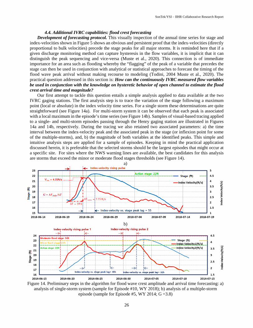
SonTek/YSI – IIHR Collaborative Research Report
26
4.4. Additional IVRC capabilities: flood crest forecasting Development of forecasting protocol. This visually inspection of the annual time series for stage and
index-velocities shown in Figure 5 shows an obvious and persistent proof that the index-velocities (directly proportional to bulk velocities) precede the stage peaks for all major storms. It is reminded here that if a given discharge monitoring method can capture hysteresis in the flow variables, it is implicit that it can distinguish the peak sequencing and vice-versa (Muste et al., 2020). This connection is of immediate importance for an area such as flooding whereby the “flagging” of the peak of a variable that precedes the stage can then be used in conjunction with analytical or statistical approaches to forecast the timing of the flood wave peak arrival without making recourse to modeling (Todini, 2004 Muste et al., 2020). The practical question addressed in this section is: How can the continuously IVRC measured flow variables be used in conjunction with the knowledge on hysteretic behavior of open channel to estimate the flood crest arrival time and magnitude?
Our first attempt to tackle this question entails a simple analysis applied to data available at the two IVRC gaging stations. The first analysis step is to trace the variation of the stage following a maximum point (local or absolute) in the index velocity time series. For a single storm these determinations are quite straightforward (see Figure 14a). For multi-storm system it can be observed that each peak is associated with a local maximum in the episode’s time series (see Figure 14b). Samples of visual-based tracing applied to a single- and multi-storm episodes passing through the Henry gaging station are illustrated in Figures 14a and 14b, respectively. During the tracing we also retained two associated parameters: a) the time interval between the index-velocity peak and the associated peak in the stage (or inflexion point for some of the multiple-storms), and, b) the magnitude of both variables at the identified peaks. This simple and intuitive analysis steps are applied for a sample of episodes. Keeping in mind the practical application discussed herein, it is preferable that the selected storms should be the largest episodes that might occur at a specific site. For sites where the NWS warning lines are available, the best candidates for this analysis are storms that exceed the minor or moderate flood stages thresholds (see Figure 14).
a)
b)
Figure 14. Preliminary steps in the algorithm for flood wave crest amplitude and arrival time forecasting: a)
analysis of single-storm system (sample for Episode #10, WY 2018); b) analysis of a multiple-storm episode (sample for Episode #5, WY 2014; G =3.8)

SonTek/YSI – IIHR Collaborative Research Report
27
Based on the assumption that passages of identical storms or individual pulses superposed on already
ongoing waves are driven by the Equation (2), we hypothesize that pulses of unsteady flows result in similar responses for a specific site. We further hypothesize that unsteady flow pulses applied to the same state of the variables produce hysteretic loops with similar characteristics. If long-term series of storm episodes are available for such tracing inspections, the results of the previously-mentioned analysis on the index-velocity and stage time series can be retained for building up the forecasting database. The longer the available records at a station, the more representative is the assembled forecasting database. Taking advantage of the six-year datasets available for this study we could trace 38 storm episodes at Henry gaging station.
Following the initial steps of the forecasting trial & error exercises, we realized that the hysteresis magnitude is not sufficiently characterized by only retaining the state of the variable at their peaks, but also on the “memory” of the flow to get to that state, as actually implied by the shear definition of hysteresis (Prowse, 1984). Consequently, we clustered the available dataset in groups using an additional parameter that takes into account not only the state of the index-velocity but also the gradient associated with its rising. This parameter, aimed to define the intensity of the storm, is labeled herein as “Flood Wave Intensity Gradient” (FWIG), defined as G = ΔVindex/ΔT, with ΔT with ΔT measured on the flood wave time series scale (hours). The parameter is associated only with the rising portion of the index-velocity hydrograph, as illustrated in Figure 14a. This parameter can easily obtained from the records of the incoming index-velocity. The values of this gradient for the 38 storms analyzed at Henry station is provided in Figure 15a, Note that the numerical value of the actual gradients are multiplied by 100 for convenience.
a) b)
Figure 15. Final steps in algorithm for flood wave crest amplitude and arrival time forecasting: a) summary storm episode analysis and establishment of Flood Wave Intensity Gradient thresholds, G; and, b) hindcast for event #10 WY 2018 (G=2.8) based on maximum index velocity “flagged” by the SonTek-
SL direct measurement (4.35 ft/s entered in the look-up table for FWIG-G2) By pairing the index-velocity state with the phase lag between the index velocity and stage and the time
lag between the index-velocity peak and the associated stage crest look-up tables can be produced for each FWIG groups. The such-obtained look-up tables are actually regression equations applied to the above two mentioned relationships. Plotted in Figure 15b are the regression equations for the FWIG-G2 zone corresponding to FWIG between 2.4 and 3.8 ft/s2. The blue line in this figure represents the functional relationships for the index-velocity peak at a given time and the lag for the associated stage crest. The green line represents the functional relationship between the index-velocity peak and the magnitude of the stage crest. Such relationships were developed for the other two FWIG zones (see Appendices A and B for Henry and Kingston Mines gaging stations). A relevant note on the numerical values of the look-up tables obtained for the Henty station is the lags between the index-velocity peaks and stages range between 5 and 68 hours

SonTek/YSI – IIHR Collaborative Research Report
28
(equivalent to 2.8 days), with larger lags and magnitudes for the flood waves of considerable size and intensity that propagate through the station.
It can be concluded that the type of stream forecasting that can be obtained from this in-stream data analysis is of the short-term nature, therefore adequate for release of warnings associated with the imminence of flood crest arrival. The ranges for the lag times and flood crest magnitudes are site-specific. Such information is useful to complement and check the weekly stream forecasts issued by the specialized meteorological agencies such as NOAA’s Advanced Hydrologic Prediction Service (http://water.weather.com). The present procedure for FWIG development is rather crude and laborious but it is considered appropriate for the present exploratory phase of this research as it can benefit for continuous scrutiny and use of intuition when needed. More efforts are requires to automate and optimize the development of such relationships using statistical and other analytical tools.
Forecasting procedure. The practical use of the forecasting approach is demonstrated by hindcasting event #1 WY 2016 illustrated in Figure 15b. Assuming that the look-up table for the forecasting are available to the station operators or other remotely located interested party, the 15-minute data is watched closely for storms that are above the flood warning lines designated by NWS. Further assuming that a forecasting software module is available to apply moving averaging over the last 5-10 incoming data points, the module can flag the occurrence of the maximum index velocity in practically real time.
Once that the maximum index-velocity peak for such a storm is detected, the value of the max velocity is entered in the look up table (that can be embedded in the software) to subsequently retrieve the values for the predicted flood crest stage and its time of arrival, as shown in Figure 15b. The predicted values for event #1 WY 2016 using the FWIG-G3 look-up table are 24.5 ft with a lag time of 76 hours. The time series for the same event, shown in Figure 14a, indicate a crest stage of 30 ft with a 75 hour lag from the index velocity peak. The agreement between the recorded and predicted values is not perfect but is close. In order to further test the capability of the proposed forecasting protocol, several storms available on records from different FWIG classes were tested for both Henry and Kingston Miles gaging station. The full results of those hindcasts are provided in Appendix A and B, respectively. The summary of the hindcasts for selected storms at Henry is shown in Table 7. The percentage differences seems to increase with the storm intensity and they are more prominent for the forecast lag them for stage estimation. It is expected that the forecast accuracy can be substantially improved with the increased number of samples for determining the look-up relationships and optimization of the base forecasting algorithms.
Table 7. Summary of the comparison between actual measurements and hindcasted values Storm episode (FWIG level)
IVRC Measurements FIWG-based Forecast Difference (%)* Stage (ft) Lag (h) Stage (ft) Lag (h) Stage Lag
#7-2018 (G1) 18 28 18 27 0.0 -3.6 #5-2016 (G1) 22 51 23 49 4.5 -3.9 #7-2016 (G2) 18 31 19 30 5.5 -3.2 #10-2018 (G2)** 22 57 23 59 2.2 -3.5 #1-2015 (G3) 20 49 19 47 0.0 -4.1 #2-2017 (G3) 18 18 18 17 0.0 -5.6
*the references are the measured values ** case analyzed in Figure 15b
5 Research finding summary & Future work The data-driven exploration conducted on SonTek-SL probes data acquired in unsteady flows is
intentionally kept in its simplest form to allow the tracing of hysteresis phenomenology and dependencies rather than cluttering the narration with analytical and statistical analysis. The fresh perspectives enabled by using this investigative approach provides useful insights on the physics of flood wave propagation in natural open channels. These insights coupled with the analytical and experimental evidence presented in this study demonstrate that:
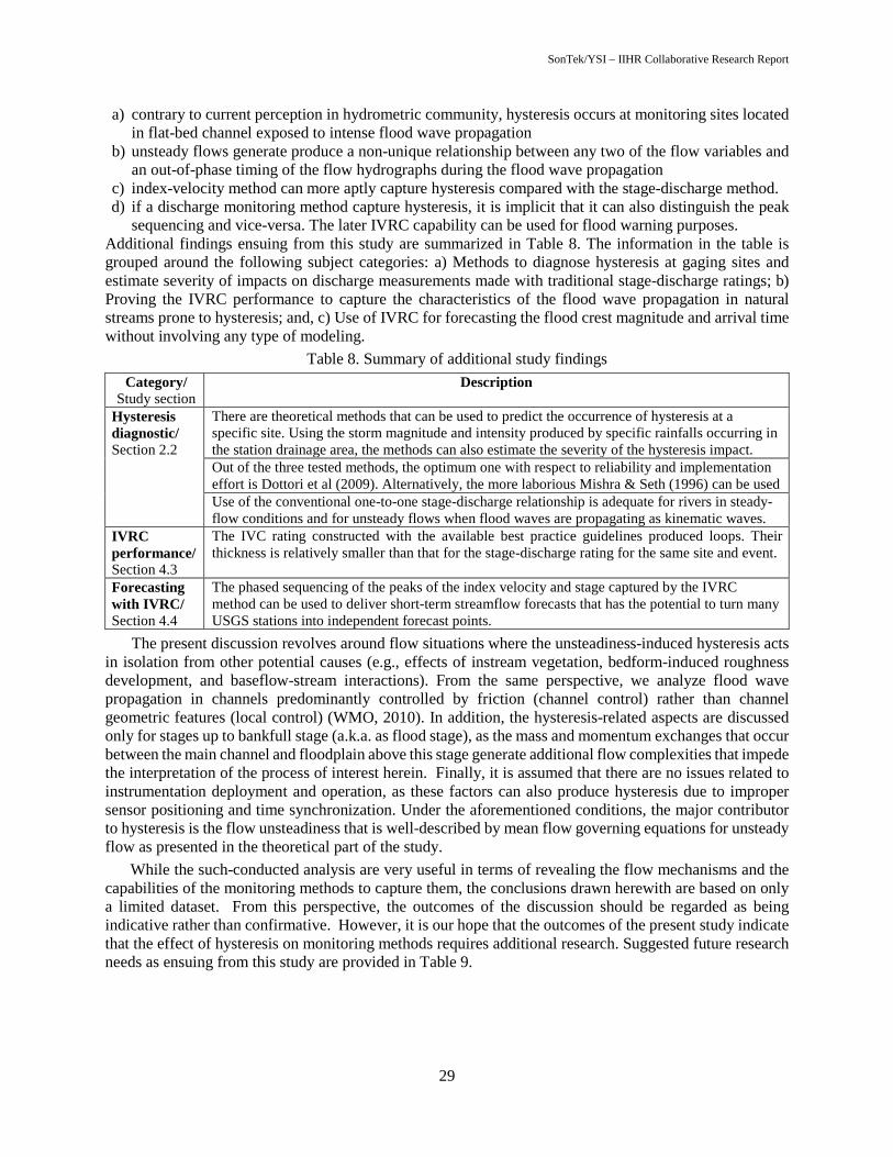
SonTek/YSI – IIHR Collaborative Research Report
29
a) contrary to current perception in hydrometric community, hysteresis occurs at monitoring sites located in flat-bed channel exposed to intense flood wave propagation
b) unsteady flows generate produce a non-unique relationship between any two of the flow variables and an out-of-phase timing of the flow hydrographs during the flood wave propagation
c) index-velocity method can more aptly capture hysteresis compared with the stage-discharge method. d) if a discharge monitoring method capture hysteresis, it is implicit that it can also distinguish the peak
sequencing and vice-versa. The later IVRC capability can be used for flood warning purposes. Additional findings ensuing from this study are summarized in Table 8. The information in the table is grouped around the following subject categories: a) Methods to diagnose hysteresis at gaging sites and estimate severity of impacts on discharge measurements made with traditional stage-discharge ratings; b) Proving the IVRC performance to capture the characteristics of the flood wave propagation in natural streams prone to hysteresis; and, c) Use of IVRC for forecasting the flood crest magnitude and arrival time without involving any type of modeling.
Table 8. Summary of additional study findings Category/
Study section Description
Hysteresis diagnostic/ Section 2.2
There are theoretical methods that can be used to predict the occurrence of hysteresis at a specific site. Using the storm magnitude and intensity produced by specific rainfalls occurring in the station drainage area, the methods can also estimate the severity of the hysteresis impact. Out of the three tested methods, the optimum one with respect to reliability and implementation effort is Dottori et al (2009). Alternatively, the more laborious Mishra & Seth (1996) can be used Use of the conventional one-to-one stage-discharge relationship is adequate for rivers in steady-flow conditions and for unsteady flows when flood waves are propagating as kinematic waves.
IVRC performance/ Section 4.3
The IVC rating constructed with the available best practice guidelines produced loops. Their thickness is relatively smaller than that for the stage-discharge rating for the same site and event.
Forecasting with IVRC/ Section 4.4
The phased sequencing of the peaks of the index velocity and stage captured by the IVRC method can be used to deliver short-term streamflow forecasts that has the potential to turn many USGS stations into independent forecast points.
The present discussion revolves around flow situations where the unsteadiness-induced hysteresis acts in isolation from other potential causes (e.g., effects of instream vegetation, bedform-induced roughness development, and baseflow-stream interactions). From the same perspective, we analyze flood wave propagation in channels predominantly controlled by friction (channel control) rather than channel geometric features (local control) (WMO, 2010). In addition, the hysteresis-related aspects are discussed only for stages up to bankfull stage (a.k.a. as flood stage), as the mass and momentum exchanges that occur between the main channel and floodplain above this stage generate additional flow complexities that impede the interpretation of the process of interest herein. Finally, it is assumed that there are no issues related to instrumentation deployment and operation, as these factors can also produce hysteresis due to improper sensor positioning and time synchronization. Under the aforementioned conditions, the major contributor to hysteresis is the flow unsteadiness that is well-described by mean flow governing equations for unsteady flow as presented in the theoretical part of the study.
While the such-conducted analysis are very useful in terms of revealing the flow mechanisms and the capabilities of the monitoring methods to capture them, the conclusions drawn herewith are based on only a limited dataset. From this perspective, the outcomes of the discussion should be regarded as being indicative rather than confirmative. However, it is our hope that the outcomes of the present study indicate that the effect of hysteresis on monitoring methods requires additional research. Suggested future research needs as ensuing from this study are provided in Table 9.

SonTek/YSI – IIHR Collaborative Research Report
30
Table 9. Summary of suggested research Research focus/
Section Description
Hysteresis diagnostic/ Section 2.2
Muste & Lee (2013) make reference to more hysteresis diagnostic formulas that need evaluation for practical purposes. Further search is needed for evaluation of optimum hysteresis diagnostic methods that are reliable and require minimum of data inputs and implementation efforts.
IVRC performance/ Sections 2.1. 4.2, 4.3
The IVRC needs evaluation for unsettled issues in the measurements of steady flows: site characteristics (changes in the cross-sectional and vertical velocity distribution), probe optimum positioning in the cross-section (in the vertical and across the stream), probe setting (measurement volume selection, duration for velocity averaging), flow and environmental conditions (presence of seasonal temperature and density gradients in the channel). Evaluation of the validity of one-to-one IVRC relationship as currently prescribed by guidelines. The present study shows that velocities profiles on the rising limb are larger than on the falling limb for the same flow depth and that the difference between profiles increases with flow unsteadiness. Evaluation of the current protocols for IVRC ratings and testing of alternative protocols for index-velocity rating construction that separately account for flow phases (i.e., rising or falling stages of hydrographs). This approach is recommended by Ruhl & Simpson (2005) for rivers located in tidal areas, whereby the IVRC regression is “segmented” to follow the flow the ebb-to-flood and flood-to-ebb flow phases.
Forecasting with IVRC/ Section 4.4
Identification of suitable methods for data-mining the IVRC-related variables for automatic detection of the phase lags between the peaks of the index-velocity and stage hydrographs and estimation of flood crest magnitude for a range of flow conditions (Muste et al., 2020).
Other research needs/ Section 3.2
Thorough uncertainty analysis using rigorous methodologies (Muste et al., 2012; Mansanarez et al., 2019). Evaluation of the accurate measurements of IVRC in unsteady flow on the assessment of flow volumes and sediment loads for suspended sediment (or any other matter in suspension) transported through gaging stations. Currently they are innacurate as they do not accound for the hysteretic effects. Evaluation of the impact of using IVRC-provided input in modeling of unsteady flows with numerical simulations (e.g., HEC-RAS with unsteady module) The unexpectedly bold illustration of the hysteretic effects at the two USGS gaging stations, reveals that there is potential for further developments of the current SonTek-SL configuration that can complement, enhance, and further expand the capabilities of the instrument to measure in steady and unsteady flows. Some of the development ideas are inspired from the current review of the present authors published in Muste et al. (2020).
6 Conclusion The present study demonstrates that currently there means to build on the existing analytical
knowledge, legacy data, and advancement in sensing and computer technologies to improve our capabilities to enhance the accuracy of the flow during unsteady flows. This type of flows is associated with each storm in the drainage area hence it potentially affect the long-term budgets of water and the loads of transported materials carried during storms. Of special significance is the impact of hysteresis in extreme events such as floods when accuracy and timeliness of the data are needed most.
Equally important is for the present study is that it convincingly demonstrate that the acoustic probes such as SonTek-SLs are reliable tools for providing accurate data in complex measurement situations and they reveal potential for further enhancing the capabilities of the index-velocity methods to support decision-making in flood mitigation efforts and beyond. These capabilities open possibility to use the monitoring methods for anticipating extreme flows if suitable analytical modules are applied to the measured data in real time.

SonTek/YSI – IIHR Collaborative Research Report
31
7. References
Aricó, C., Nasello, C., and Tucciarelli, T. (2009), Using unsteady state water level data to estimate channel roughness and discharge hydrograph, Adv. Water Resour., 32, 1223–1240, doi:10.1016/j.advwatres.2009.05.001.
Bares, V., Jirak, J. and Pollert, J. (2008). Spatial and temporal variation of turbulence characteristics in combined sewer flow, Flow Measurement and Instrumentation 19, 145-154.
Boldt, J. A. and Oberg, K. A. (2015). Validation of stream_flow measurements made with M9 and RiverRay acoustic Doppler current profiler, J. Hydraulic Engineering, 142, 04015054, 16p.
Cabrera, R., Deines, K., Brumley, B. and Terray, E. (1987). Development of a practical coherent acoustic Doppler current profiler, in Proc. Oceans ’87, pp. 93-97
Carter, R. W. and Anderson, I. E. (1963). Accuracy of current meter measurements. J. Hydr. 736 Div., 89(4), 105–115. 737
Chen, Y-C., Yang, T-M., Hsu, N-S. and Kuo, T-M. (2012). Real-time discharge measurement in tidal streams by an index velocity, Environ, Monit Assess (184, 6423-6436.
Cheng, Z., Lee, K., Kim, D., Muste, M., Vidmar, P. and Hulme, J. (2019). Experimental Evidence on the Performance of Ratting Curves for Continuous Discharge Estimation in Complex Flow Situations, J. of Hydrology, https://doi.org/10.1016/j.jhydrol.2018.11.021, pp. 959-971
Chiu C-L. and Chen, Y-C. (2003). An efficient method of discharge estimation based on probability concept. Journal of Hydraulic Research 41(6), 589–596.
Chow, V.T. (1959). Open channel Flow, McGrow Hill, New York, NY. Di Baldassarre, G. and Montanari, A. (2009). “Uncertainty in River Discharge Observations: A Quantitative
Analysis,” Hydrol. Earth Syst. Sci. Discuss., 6, pp. 39–61. Dottori, F., Martina, L.V., and Todini, E. (2009). “A Dynamic Rating Curve Approach to Indirect Discharge
Measurements,” Hydrol. Earth Syst. Sci, 13, pp. 847-863. Eberts, S.M., Woodside, M.D., Landers, M.N., and Wagner, C.R. (2019). Monitoring the pulse of our Nation's rivers
and streams—The U.S. Geological Survey streamgaging network: U.S. Geological Survey Fact Sheet 2018–3081, 2 p., https://doi.org/10.3133/fs20183081.
Faye, R.E. and Cherry, R.N. (1980). Channel and Dynamic flow characteristics of the Chattahoochee River, Buford Dam to Georgia Highway 141, Geological Survey Water-supply Paper 2063, U.S. Government Printing Office, Washington, DC
Ferrick, M.G. (1985). Analysis of river wave types, Water Resources Research, 21(2), 209-220. Fread, D.L. (1975). “Computation of Stage-Discharge Relationships Affected by Unsteady Flow,” Water Resources
Bulletin, 11(2), pp. 213-228. Fread, D.L. (1985). Channel routing. M.G. Anderson, T.P. Burt (Eds.), Hydrological Forecasting, Wiley, New York. Friedman, J.H. (1984). A variable span smother, Technical Report PUB-3477, Laboratory for Computational
Statistics, Stanford University, Stanford, CA. Gonzalez-Castro, J.A. and Chen, Z. (2015). Uncertainty of index-velocity measurements at culverts, Proceedings
World Water and Environmental Resources Congress. May 15-19, Anchorage, AK. Gosh, S. (2014). Flood control and drainage engineering, 4th Edn., Oxford& IBH Publishing Company Pvt.
Limited. Graf, W.H. and Suszka, L., 1985. Unsteady flow and its effect on sediment transport. Proceedings of the 21st
Congress, IAHR, Melbourne, Australia, 1–5. Graf, W.H. and Qu, Z. (2004). “Flood Hydrographs in Open Channels,” Proceedings of the Institute of Civil
Engineers Water Management (157), pp. 45-52. Fread, D.L. (1975). Computation of Stage-Discharge Relationships Affected by Unsteady Flow, Water Resources
Bulletin, 11(2), pp. 213-228. HEC (2008). Hydraulic Engineering Centre (HEC): Hydraulic Reference Manual.U.S. Army Corps of Engineers,
Davis, California, USA. Henderson, F.M. (1966). Open Channel Flow. Macmillan Series in Civil Engineering, Macmillan Company, New
York, 522 pages Herschy, R. (2009). Streamflow measurement (3d ed.). Oxford: Taylor & Francis. Holmes, R.R., (2016). River rating complexity, Proceedings River Flow Conference, St. Louis, MO, Taylor &
Francis Group, ISBN 978-1-138-02913-2 Huang, H., 2012.Uncertainty Model for In Situ Quality Control of Stationary ADCP Open-Channel Discharge
Measurement. J. Hydraul. Eng. 138(1), 4-12

SonTek/YSI – IIHR Collaborative Research Report
32
Hunt, A.E., (1997). The behavior of turbulence in unsteady open channel flow. PhD Thesis, University of Canterbury, New Zealand.
Hidayat, H., Vermeulen, B., Sassi, M. G., Torfs, P. J. J. F. and Hotink, A. J. F., (2011). Discharge estimation in a backwater affected meandering river. Hydrol. Earth Syst. Sci., 15, 2717-2728, doi:10.5194/hess-15-2717-2011.
Jackson, P.R., Johnson, K.K. and Duncker, J.J., (2012). Comparison of index velocity measurements made with a horizontal acoustic Doppler current profiler and a three-path acoustic velocity meter for computation of discharge in the Chicago Sanitary and Ship Canal near Lemont, Illinois: U.S. Geological Survey Scientific Investigations Report. 2011–5205, 42 p.
Jones, B.E. (1916). A method of correcting river discharge for a changing stage, Water Supply Paper 375, U.S. Geological Survey, p. 117-130
Julien, P. Y. (2002). River mechanics, Cambridge University Press, Cambridge, UK. Kennedy, E.J., 1984, Discharge ratings at gaging stations: U.S. Geological Survey Techniques of Water-Resources
Investigations, book 3, chap. A10, 59 p. (http://pubs.usgs.gov/twri/twri3-a10/.) Lamberti, P. and Pilati, S. (1990). Quasi-kinematic flood wave propagation, Meccanica, 25, 107-114. Le Coz, J., Pierrefeu, G. and Paquier, A. (2008). Evaluation of river discharges monitored by a fixed side-looking
Doppler profiler, Water Resources Research 44 p. 1-13. Levesque, V.A., and Oberg, K.A., 2012, Computing discharge using the index velocity method: U.S. Geological
Survey Techniques and Methods 3–A23, 148 p. (Available online at http://pubs.usgs.gov/tm/3a23/) Kastner, K., Hoitink, A.J.F., Torfs, P.J.J.F., Vermuelen, B., Ningshi, N.S. and Pramulya, M. (2018). Prerequisities
for accurate monitoring of river discharge based on fixed-location velocity measurements. Water Resour. Res., 54. https://doi.org/10.1002/2017WR020990.
Knight, D.W., 2006. River flood hydraulics: calibration issues in one-dimensional flood routing models. In: Knight DW, Shamseldin AY (eds) Chapter 18 in River basin modelling for flood risk mitigation, Taylor & Francis, Chichester, 335–385
Mallakpour, I., and G. Villarini (2015). The changing nature of flooding across the central United States, Nature Climate Change, 5, 250-254.
Mansanarez, V., Westerberg, I. K., Lam, N., and Lyon, S. W. (2019). Rapid Stage‐Discharge Rating Curve Assessment Using Hydraulic Modeling in an Uncertainty Framework. Water Resources Research, 55, 9765–9787. https://doi.org/10.1029/2018WR024176
Messner, F. and Meyer, V. (2006) Flood damage, vulnerability and risk perception - challenges for flood damage research. In: Schanze, J., Zeman, E. and Marsalek, J. (eds) Flood Risk Management: Hazards, Vulnerability and Mitigation Measures, 67, 149-167.
Mishra, S.K. and Seth, S.M., 1996. Use of hysteresis for defining the nature of flood wave propagation in natural channels. Hydrological Sciences-Journal-des Sciences Hydrologiques 41(2), 153–170.
Morlock, S.E., Nguyen, H.T. and Ross, J. (2002). Feasibility of Acoustics Doppler Velocity meters for the production of discharge records from U.S. Geological Survey Stream-flow-Gaging Stations, U.S.G.S. Water-resources Investigations Report, Indiannapolis, IN.
Morse, B., Richard, M., Hamai, K., Godin, D., Choquette, Y. and Pelletier, G. (2010). Gauging rivers during all seasons using the Q2D velocity index method, J. Hydraulic Engineeering, 136(4), 195-203.
Moussa, R. and Bocquillon, C. (1996). Criteria for the choice of flood-routing methods in natural channels, J. Hydrol. 186, 1-30.
Moots, E.E. (1927). A study in flood waves, University of Iowa Studies in Engineering, Bulleting No. 14, PhD thesis dissertation State University of Iowa, Iowa City, IA.
Moramarco, T., Pandolfo, C. and Singh, V.P. (2008b). Accuracy of kinematic wave and diffusion wave approximations for flood routing. I: Steady analysis, J. Hydrologic Engineering, 13(11), 1078-1088.
Moramarco, T., Pandolfo, C. and Singh, V.P. (2008b). Accuracy of kinematic wave and diffusion wave approximations for flood routing. II: Unsteady analysis, J. Hydrologic Engineering, 13(11), 1089-1096.
Mrokowska, M.M., Rowinski, P.M. and Kalliowska, M.B. (2015). A methodological approiach of estimating resistance to flow under unsteady flow conditions, Hydrol, Earth Syst. Sci. 19, 4041-4053, doi: 10.5194/hess-19-4041-2015
Mueller, D.S., Abad, J.D., García, C.M., Gartner, J.W., García, M.H., and Oberg, K.A., 2007. Errors in Acoustic Doppler Profiler Velocity Measurements Caused by Flow Disturbance. J. Hydraul. Eng. 133(12), 1411-1420.

SonTek/YSI – IIHR Collaborative Research Report
33
Muste, M., Lee, K. and Bertrand-Krajewski, J-L. (2012). Standardized Uncertainty Analysis Frameworks for Hydrometry: Review of Relevant Approaches and Implementation Examples, Hydrological Sciences Journal, available on line; doi:10.1080/0262667.2012.675064.
Muste, M. and Lee, K. (2013). “Evaluation of Hysteretic Behavior in Streamflow Rating Curves,” Proceedings 2013 IAHR Congress, Chengdu, September 8-13, Tsinghua University Press, China.
Muste, M., Cheng, Z., Vidmar, P. and Hulme, J. (2015). Considerations on Discharge Estimation Using Index-Velocity Rating Curves, Proceedings 36th IAHR World Congress, 28 June – 3 July, The Hague, The Netherlands.
Muste, M., Cheng, Z., Firoozfar, A.R., Tsai, H-W., Loeser, T. and Xu, H. (2016). “Impacts of Unsteady Flows on Monitoring Stream Flows,” River Flow Conference, July 12-15, 2016, St Louis, MO, USA.
Muste, M. and Hoitink, T. (2017). “Measuring Flood Discharge”, Chapter in “Oxford Research Encyclopedia of Natural Hazard Science”, Subject: Case Studies, Risk Assessment, Vulnerability, Floods, Oxford University Press, doi: 10.1093/acrefore/9780199389407.013.121
Muste, M., Bacotiu, C. and Thomas, D. (2019). Evaluation of the slope-area method for continuous streamflow monitoring, Proceedings of the 38th World Congress, September 1-6 2019, Panama City, Panama.
Muste, M., Lee, K., Kim, D., Bacotiu, C., Rojas-Oliveros, M. and Cheng, Z. (2020a). Revisiting hysteresis of flow variables in monitoring unsteady streamflows, Journal of Hydraulic Research (in press)
Nezu, I., Kadota, A., Nakagawa, H. (1997). Turbulent structure in unsteady depth-varying open-channel flows, J. Hydra. Eng., ASCE, 110, 173-193.
Nezu, I. and Nakagawa, H., (1994). Turbulence measurements in unsteady free-surface flows, Flow Meas. Instrument., 6(1), 49-59, doi: 10.1016/0955-5986(95)93458-7
Nihei, Y. and Sakai, T. (2006). Study of river-discharge measurements with a bottom-mounted ADCP, Proceedings River Flow International Conference on Fluvial Hydraulics, Lisbon, Portugal; 6-8 September 2006; Eds. Alves, E.C.T.L., Cardoso, A.H., Leal, J.G.A.B. and Ferreira, R.M.L.; Taylor and Francis.
Nihei, Y. and Kimizu, A. (2008). A new monitoring system for river discharge with horizontal acoustic Doppler current profiler measurements and river simulations, Water Resources Research, 44, doi: 10.1029/2008WRR006970.
Patino, E. and Ockerman, D. (1997). Computation of mean velocity in open channels using acoustic velocity meters, U.S. Geological Survey Opeb-File Report 97-220.
Pelletier, P. M., (1988). Uncertainties in the single determination of river discharge: A literature 833 review. Can. J. Civ. Eng., 15(5), pp. 834–850.
Perumal, M., Sherestha, K. B., and Chaube, U. C. (2004). Reproduction of hysteresis in rating curves, J. Hydraul. Eng.-ASCE, 130, 870–878, doi: 10.1061/(ASCE)0733-9429(2004)130:9(870).
Ponce, V.M. and Simon, D.B., 1977. Shallow water propagation in open channel flow. J.Hydr. Div., 103, 1461–1476.
Ponce, V.M., 1989. Engineering Hydrology Principles and Practices. Prentice Hall, Englewood Cliffs, NJ. Prowse, C.W. (1984). Some thoughts on lag and hysteresis, Royal Geographical Society, 16(1), 17-23. Qu, Z., 2003. Unsteady open-channel flow over a mobile bed. PhD Thesis, Ecole Polytechnique Federale de
Lausanne, Lausanne, Switzerland. Rantz, S.E. and others, (1982). “Measurement and computation of streamflow”. US Geological Survey Water
Supply Paper 2175, 1, 2. RDI (1989). Acoustic Doppler Current Profilers - Principles of Operation: A Practical Primer, RD Instruments, San
Diego, CA.Rennie, C., Hoitink, A.J.F., and Muste M. (2017). Chapter 6 in Experimental Hydraulics, Volume II; J. Aberle, C.D. Rennie, D.M. Admiraal, M. Muste (Editors); Taylor & Francis, New York, NY.
Ruhl, C.A., and M.R. Simpson (2005), “Computation of discharge using the index-velocity method in tidally affected areas”. U.S. Geological Survey, Scientific Investigations Report 2005-5004, Reston, VA.
Saint-Venant, A.J.C. Barré de (1871), "Théorie du mouvement non permanent des eaux, avec application aux crues des rivières et a l'introduction de marées dans leurs lits", Comptes Rendus de l'Académie des Sciences, 73: 147–154 and 237–240
Schmidt, A. R. (2002). “Analysis of Stage-discharge Relations for Open Channel Flows and their Associated Uncertainties.” Ph.D. Thesis, U of Illinois at Urbana-Champaign, Champaign, IL
Shen, Y. and Diplas, P. (2010). Modeling unsteady flow characteristics for hydropeaking operations and their implications on fish habitat, J. Hydraul. Eng.-ASCE, 136, 1053–1066, doi:10.1061/(ASCE)HY.1943-7900.0000112.
Song, T. & Graf, W. H. (1996) Velocity and turbulence distribution in unsteady open-channel flows. J. Hydraul. Engng ASCE 122(3), 141-154.

SonTek/YSI – IIHR Collaborative Research Report
34
SonTek/YSI (2000). Acoustic Doppler profiler principles of operation: San Diego, CA, SonTek/YSI, 28 p. Todini, E. (2004). “Role and Treatment of Uncertainty in Real-time Flood Forecasting” Hydrological Processes
(18), pp. 2743–2746 World Meteorological Organization (2010). Manual on stream gauging, Volume I, Field Work. WMO No. 1044.
Available at: www.wmo.int/pages/prog/hwrp/publications/stream_gauging/1044_Vol_I_en.pdf Yang, S.Q. and Chow, A., (2008). Turbulence structures in non-uniform flows. Advances in Water Resources, 31,
pp. 1344-1351. ANNEX A: Testing the hysteresis diagnostic formulas for the USGS stations at Henry gaging station (#05558300) ANNEX B: Testing the hysteresis diagnostic formulas for the USGS stations at Kingston Miles gaging station
(#05568500)