AUFLS II - Appendix A - Transpower New Zealand · It is important that the frequency remains close...

AUFLS II - Appendix A

An Introduction to Reserve Management Concepts and AUFLS

System Operator

4/08/2011

System Operator Report: AUFLS II - Appendix A of 18

NOTICE

COPYRIGHT © 2011 TRANSPOWER New Zealand LIMITED

ALL RIGHTS RESERVED The information contained in the report is protected by copyright vested in Transpower New Zealand Limited (“Transpower”). The report is supplied in confidence to you solely for your information. No part of the report may be reproduced or transmitted in any form by any means including, without limitation, electronic, photocopying, recording, or otherwise, without the prior written permission of Transpower. No information embodied in the report which is not already in the public domain shall be communicated in any manner whatsoever to any third party without the prior written consent of Transpower.

Any breach of the above obligations may be restrained by legal proceedings seeking remedies including injunctions, damages and costs.

LIMITATION OF LIABILITY/DISCLAIMER OF WARRANTY Transpower make no representation or warranties with respect to the accuracy or completeness of the information contained in the report. Unless it is not lawfully permitted to do so, Transpower specifically disclaims any implied warranties of merchantability or fitness for any particular purpose and shall in no event be liable for, any loss of profit or any other commercial damage, including but not limited to special, incidental, consequential or other damages.

Position Date

Prepared By: System Operator 4/8/2011

Reviewed By:


TABLE OF CONTENTS 1 PLANNING FOR UNDER FREQUENCY EVENTS ................................................................................................. 4

1.1 Normal Frequency Fluctuations ........................................................................................ 4 1.2 Contingent Events ............................................................................................................ 4 1.3 Large Rare System Events ............................................................................................... 5 1.4 Manage System Collapse ................................................................................................. 6

2 HOW DOES THE SYSTEM OPERATOR PROCURE RESERVES? ........................................................................... 7 2.1 Overview of The Reserve Management Tool ................................................................... 7

3 WHAT EVENTS WILL AUFLS COVER? ......................................................................................................... 10 4 CONSEQUENCES OF UNDER-FREQUENCY EVENTS ........................................................................................ 13

4.1 Normal Frequency Fluctuations ...................................................................................... 13 4.2 Contingent Events .......................................................................................................... 13 4.3 Large Rare System Events ............................................................................................. 14 4.4 System Collapse ............................................................................................................. 16 4.5 Overview of Consequences ............................................................................................ 18


An Introduction to Reserve Management Concepts and AUFLS

To understand the role and purpose of AUFLS it is helpful to know the basic concepts of power system reserve management. The following section aims to provide an overview of how the System Operator plans to prevent under frequency events, why AUFLS exists, and where AUFLS fits in the wider scheme of under frequency management.

1 Planning for Under Frequency Events

1.1 Normal Frequency Fluctuations

Power supply must be carefully balanced with demand in order to keep our power system stable. When power supply is balanced with demand the system frequency is 50 Hz.

It is important that the frequency remains close to 50 Hz for operational, security and quality of supply reasons. For example, some industrial processes rely on the frequency staying close to 50 Hz. Generators are also only capable of operating within a certain frequency range. This range varies between generation types.

When there is an imbalance in supply and demand, the system frequency moves away from 50 Hz. Excess demand will cause the frequency to drop (known as under-frequency). Excess supply will cause the frequency to rise (known as over-frequency).

The level of electricity demand varies considerably from one minute to the next, causing frequency fluctuations. Frequency keeping reserves assist in maintaining the system frequency within a specific band during normal operation of the power system.

A number of generating stations in each island are contracted to provide frequency keeping services, to deal with small fluctuations in frequency. These generators with spare capacity and fast response time attempt to maintain the frequency within the normal band of 49.8 Hz and 50.2 Hz.

1.2 Contingent Events

The sudden disconnection of a large generating unit is a typical example of a system event that will cause the system frequency to drop below 50 Hz. The balance can be restored by either increasing supply (generation) or decreasing demand (commonly referred to as load).

In New Zealand the System Operator procures reserves to ensure that the frequency does not drop below 48 Hz in certain types of events (known as contingent events1) and to ensure that the frequency returns to 50Hz.

Contingent events are events that happen regularly enough2 that it is important that we have sufficient reserves available to restore the system frequency to 50 Hz without impacting on end-users3. Typical examples of contingent events are the loss of a generating unit or the loss of one of the poles of the HVDC link.

1 Contingent events (CE) and extended contingent events (ECE) are defined in the System Operator‟s Policy

Statement found in Schedule C4 Part C clause 12.4. 2 As at April 2010, we have had an average of 14 such events a year over the last 3 years

3 Except for those end-users who have a contract to provide interruptible load. These end-users are paid for this

service through the IR market.


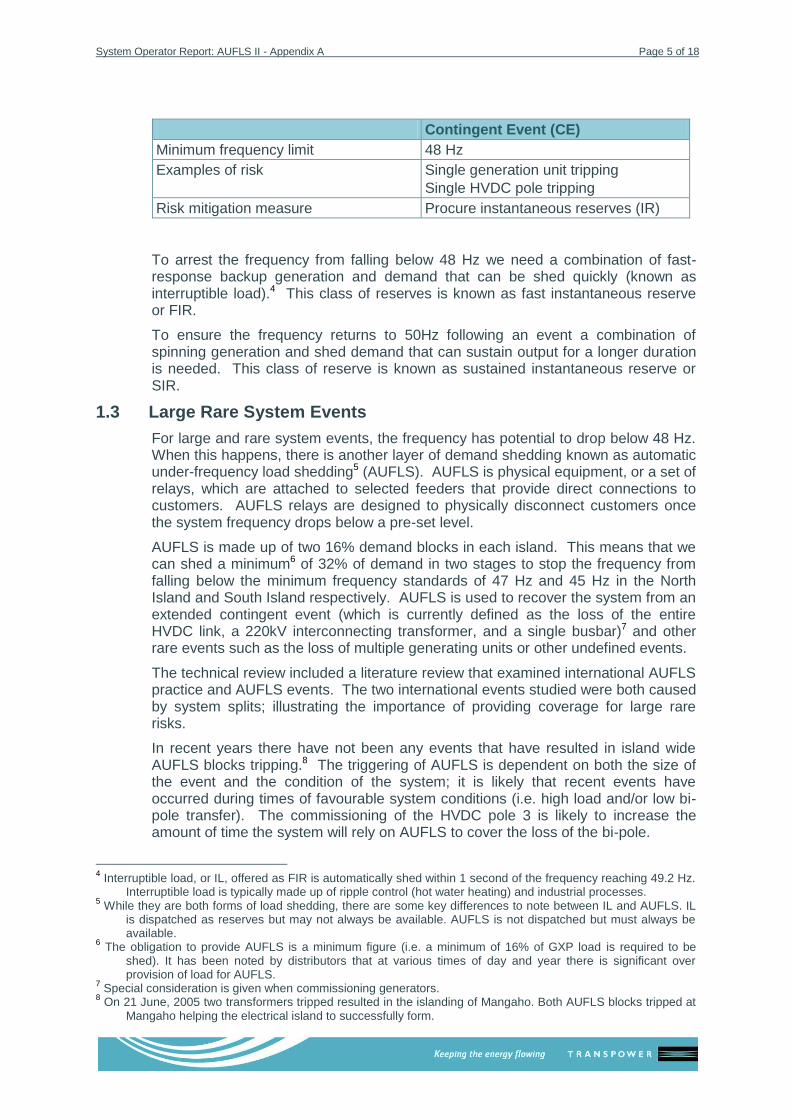
Contingent Event (CE)

Minimum frequency limit 48 Hz

Examples of risk Single generation unit tripping

Single HVDC pole tripping

Risk mitigation measure Procure instantaneous reserves (IR)

To arrest the frequency from falling below 48 Hz we need a combination of fast-response backup generation and demand that can be shed quickly (known as interruptible load).4 This class of reserves is known as fast instantaneous reserve or FIR.

To ensure the frequency returns to 50Hz following an event a combination of spinning generation and shed demand that can sustain output for a longer duration is needed. This class of reserve is known as sustained instantaneous reserve or SIR.

1.3 Large Rare System Events

For large and rare system events, the frequency has potential to drop below 48 Hz. When this happens, there is another layer of demand shedding known as automatic under-frequency load shedding5 (AUFLS). AUFLS is physical equipment, or a set of relays, which are attached to selected feeders that provide direct connections to customers. AUFLS relays are designed to physically disconnect customers once the system frequency drops below a pre-set level.

AUFLS is made up of two 16% demand blocks in each island. This means that we can shed a minimum6 of 32% of demand in two stages to stop the frequency from falling below the minimum frequency standards of 47 Hz and 45 Hz in the North Island and South Island respectively. AUFLS is used to recover the system from an extended contingent event (which is currently defined as the loss of the entire HVDC link, a 220kV interconnecting transformer, and a single busbar)7 and other rare events such as the loss of multiple generating units or other undefined events.

The technical review included a literature review that examined international AUFLS practice and AUFLS events. The two international events studied were both caused by system splits; illustrating the importance of providing coverage for large rare risks.

In recent years there have not been any events that have resulted in island wide AUFLS blocks tripping.8 The triggering of AUFLS is dependent on both the size of the event and the condition of the system; it is likely that recent events have occurred during times of favourable system conditions (i.e. high load and/or low bi-pole transfer). The commissioning of the HVDC pole 3 is likely to increase the amount of time the system will rely on AUFLS to cover the loss of the bi-pole.

4 Interruptible load, or IL, offered as FIR is automatically shed within 1 second of the frequency reaching 49.2 Hz.

Interruptible load is typically made up of ripple control (hot water heating) and industrial processes. 5 While they are both forms of load shedding, there are some key differences to note between IL and AUFLS. IL

is dispatched as reserves but may not always be available. AUFLS is not dispatched but must always be available.

6 The obligation to provide AUFLS is a minimum figure (i.e. a minimum of 16% of GXP load is required to be

shed). It has been noted by distributors that at various times of day and year there is significant over provision of load for AUFLS.

7 Special consideration is given when commissioning generators.

8 On 21 June, 2005 two transformers tripped resulted in the islanding of Mangaho. Both AUFLS blocks tripped at

Mangaho helping the electrical island to successfully form.


The most recent events of a widespread tripping of AUFLS were:

3 March 1996 - AUFLS tripped following an HVDC bi-pole tripping 9 March 1993 – AUFLS tripped following an HVDC bi-pole tripping. 6 February 1987 – AUFLS tripped following a generator circuit breaker failure at

Whakamaru. 1 June 1984 – Otahuhu-Whakamaru circuit fault triggered both manual and

automatic load shedding.

Two of the AUFLS events in New Zealand‟s history have been caused by rare risks other than bi-pole trippings which again reiterates the importance to ensure the system is equipped with an effective robust AUFLS scheme.

Extended contingent events (ECE) are expected to occur much less frequently than contingent events and therefore it is deemed to be not cost effective to procure reserves alone to cover an ECE. To cover an ECE risk the System Operator relies on both AUFLS and instantaneous reserves.

Extended Contingent Event (ECE)

Minimum frequency limit 47 Hz (North Island)

45 Hz (South Island)

Examples of risk HVDC bi-pole tripping

Loss of single bus bar

Risk mitigation measure Procure instantaneous reserves, and

Rely on AUFLS

Under the current AUFLS scheme, an event that causes the frequency to fall below 47.8 Hz will trigger a minimum of 16% of the North Island demand to be shed (47.5 Hz in the South Island). The event results in loss of supply to all customers connected on a feeder with an AUFLS stage 1 relay. If the frequency continues to fall below 47.5 Hz or remains at 47.8 Hz long enough the second block of AUFLS will trip resulting in an additional 16% of the North Island load being shed.

1.4 Manage System Collapse

AUFLS is the last response that we have available to correct the power system from collapse on under-frequency. If the AUFLS response is insufficient to correct the imbalance the frequency will continue to fall below the levels that generators can continue to safely operate.

At 47 Hz, combined cycle gas turbines and wind generators will typically disconnect which further exacerbates the situation. All generation will likely disconnect shortly after the frequency falls below 45 Hz.9 This continual disconnection of supply is known as cascade failure. Eventually the imbalance between supply and demand will be so severe that supply is lost to the entire island or fragmented with small generation electrical islands remaining. This is more commonly known as a blackout.

Generating stations in the North and South Islands are contracted by the System Operator to provide Black Start services which will assist electricity supply being re-established in the event of a blackout. Under these contracts, generating companies make available equipment needed to energise or liven the grid at grid injection points, without any power being obtained from the grid.

9 Most hydro stations will not instantly trip off at 45Hz, but will likely trip off when the frequency is below 45Hz.


2 How Does the System Operator Procure Reserves?

The AUFLS scheme is taken into account when System Operator procures reserves to cover the ECE risk. Accordingly, any changes to the AUFLS scheme may have an effect on the amount of reserves procured and the resulting cost of reserves in New Zealand. This section outlines how the reserves are procured and the implication AUFLS has on their procurement.

2.1 Overview of The Reserve Management Tool

The System Operator uses the Reserve Management Tool (RMT) and Scheduling Pricing and Dispatch (SPD) Tool to ensure that a sufficient amount of reserves is procured to cover system risks in a least cost manner. To ensure a lowest cost solution, SPD utilises the interconnection between energy and reserves to co-optimise the energy and reserve requirements.

RMT is used to ensure that there is sufficient fast reserve (FIR) available to arrest the frequency from reaching the targeted limits and sufficient sustained reserve (SIR) available to restore the frequency following a contingent or extended contingent events on the system.10

In order to procure sufficient reserves, RMT identifies the CE risks and the ECE risks on the system for each trading period. RMT identifies two types of CE risks; the first is the AC CE risk (often the loss of largest single generating unit) and second is the DC CE risk (loss of a single HVDC pole). RMT currently calculates the ECE risk as the loss of the HVDC bi-pole.11

The DC CE risk is not simply the loss of the MW transferred on a single HVDC pole. The HVDC, when running more than one pole, has the ability to ramp up its output following the loss of one of the poles.12 This is known as the DC risk subtractor and it is taken into consideration when calculating the DC CE risk.

RMT uses a model of the electrical system to calculate the reserve requirements. RMT simulates the identified risk plant tripping and models the response of the system to the shortfall in generation. The amount of fast reserve for each risk will generally not equal the size of the risk as RMT takes into account several factors including system inertia13 and the performance characteristics of the DC link. The system inertia and DC frequency response affect frequency decay and can lessen the amount of reserve required to be purchased. The affect of these system conditions is known as Net-Free Reserve (NFR).

When simulating the loss of the ECE risk, RMT takes into account the AUFLS scheme and the amount of AUFLS load available.14 RMT calculates the amount of reserve required for each risk so that the frequency reaches the frequency target (48 Hz for CE, 47/45 Hz for ECE in North/South Island respectively) and remains within the required frequency targets. The quantity of NFR is equal to the amount of calculated reserve required subtracted from the risk. Figure 3-1 outlines the calculation of NFR.

10

Sustained reserve for CE risks are procured on a 1 for 1 basis (i.e. amount of SIR equates to the risk size). This is not the case for ECE SIR however as it takes other factors into account.

11 During generator commission the unproven plant is considered a secondary ECE in addition to the bipole.

12 For a more detailed description see the Instantaneous Reserve Review work of the UFM project.

13 System inertia is the braking effect of the system particularly caused from generators.

14 RMT used an estimated minimum amount of AUFLS provision and subtracts exempted load from the

calculation.


Figure 2-1 Representation of the NFR calculation of the FIR ECE risk

Figure 2-1 displays a graphical representation of the effect of NFR on the amount of FIR required to cover an ECE risk, in this case the HVDC bipole.

Figure 2-2 Overview of calculation of NFR values for different risk types

Figure 2-2 displays an overview of the FIR calculation across the different risk types. The figure demonstrates that the largest risk does not necessarily require the most reserve to be procured.

The NFR values and reserve type for each risk are sent to SPD along with the DC risk subtractor. SPD calculates the amount of fast and sustained reserve required from the NFR values and then co-optimises the quantity of energy and reserves. To do this the market iterates between RMT, which produces the NFRs and DC ramp rates for SPD, and SPD, which produces dispatches for RMT until a lowest cost solution has been found. SPD then procures the amount of reserve needed. One risk sets the quantity of reserves that are procured; this risk is known as the binding risk. Different risks can set the FIR and SIR levels.


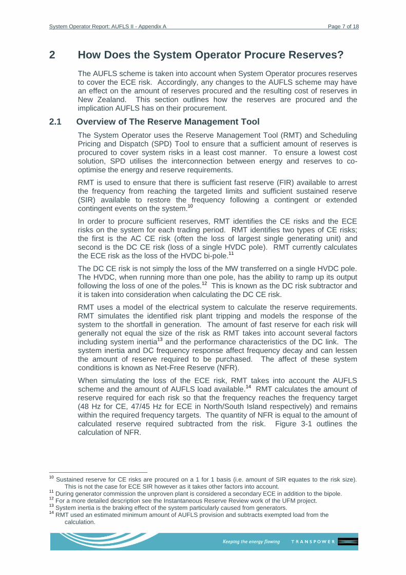
Figure 2-3 Calculation of the required amount FIR calculated by SPD

Figure 2-3 illustrates how SPD procures reserves, the AC CE risk in this case would be the binding risk and the amount of FIR required to cover the AC CE risk would be procured.

It is noted that even though a CE or ECE risk is not „the binding risk‟ these risks are still covered as enough reserves have been procured already to cover the risks should occur. This way there are sufficient reserves for all credible risks. The System Operator procures reserves to cover only one risk at a time, therefore reserves are not procured to cover for an AC CE and DC ECE occurring together as whilst such an event is possible it does not occur frequently. The cost of covering this type of event is so large that it is not classified as a credible event.15

Since the AUFLS scheme is used in the calculation of the amount of reserve required for ECE events, the amount of AUFLS load that is available and the design of the AUFLS scheme can impact the amount of reserves procured and therefore the cost of electricity. The cost benefit analysis will utilise this concept to compare potential AUFLS schemes.

It is difficult to estimate the amount of time the ECE will be the binding risk in the future.16 However once the HVDC Pole 3 is commissioned, it is likely that the ECE risk will bind more frequently therefore it is important to ensure that there is an efficient AUFLS scheme.

15

Sympathetic trips are covered during generator commissioning. 16

The use of Pole 1 has varied with different offers which make it difficult to use when forecasting future trends.


3 What events will AUFLS cover?

To better understand the role of AUFLS in the power system, the following section discusses the capability of AUFLS to cover large events.

Should AUFLS be expected to cover all large events?

While AUFLS is seen as a “safety-net” for the power system, it does not provide protection from risks of any size. There are several factors that limit the reach of the AUFLS safety net. For example, for an AUFLS scheme to be effective it needs to shed the optimum amount of load to cover events on the system and return the system to an operable frequency. As events on the system can vary in size, if AUFLS blocks are very large (ie. 2 x 25%) to cover only for the larger event then events of smaller magnitudes could result in excess load being shed. This, in turn, may cause over-frequency and potentially system collapse. In light of this and other factors, such as the band of AUFLS operation, there is a limit to the size of events that AUFLS can cover.

What events can AUFLS cover?

It is important to note that AUFLS does not exist to just cover the ECE risk, but the ECE risk is the only risk where action is taken to mitigate the risk. A loss of an ECE risk which results in the tripping of AUFLS is expected to occur 1 in 5 years while other risks are believed to occur at a less frequent rate. Events that are lower in probability are not categorised as ECEs, which means that the System Operator does not procure additional reserves to ensure the system remains intact following these events. Instead it is acknowledged that these events may or may not be covered by AUFLS. The AUFLS scheme, with the assistance of the reserves already procured and system conditions, is likely to provide some protection against low probability events but there is no certainty that the system will remain intact following such events.

Figure 3-1 Estimated level of AUFLS safety net coverage

MW

ESTIMATED LEVEL

OF COVERAGE

PROVIDED BY

AUFLS AND

RESERVES


Figure 3-1 provides a simplified graphical example to illustrate the additional safety net that is provided by AUFLS. In the example provided, the ECE risk is not the risk setter so the FIR procured in addition to the response of the system and AUFLS load create a safety net which can provide coverage for a risk larger than the ECE risk. This is especially important at times when the ECE risk is itself small compared to the other risks on the system, as illustrated in Figure 3-1.

Figure 3-2 Estimated level of AUFLS coverage during low ECE risk

Figure 3-2 illustrates that when the ECE is not the binding risk it is still important to have all AUFLS load available. If all the AUFLS load was not present it could lead to system collapse following events that the scheme would otherwise be able to cover. Maintaining constant provision of AUFLS load provides the most coverage for these rarer events.

MW

ESTIMATED LEVEL

OF COVERAGE

PROVIDED BY

AUFLS AND


Figure 3-3 Estimated level of AUFLS coverage when the ECE is the binding risk

When the ECE risk sets the amount of reserves procured then the system is not able to cope with any event greater in magnitude than the ECE risk; in effect there is no additional safety-net. Figure 3-3 provides a simplified overview of the concept in which the ECE is binding and is setting the limit for size of risk the system can cover

The coverage of other events provided by AUFLS is not monitored and the size of unknown risk capable of being covered will change with system conditions. AUFLS will not provide coverage against all system events but to provide maximum benefit of the AUFLS load and scheme it is important that AUFLS is provided at all times.

MW

ESTIMATED LEVEL

OF COVERAGE

PROVIDED BY

AUFLS AND


4 Consequences of Under-Frequency Events

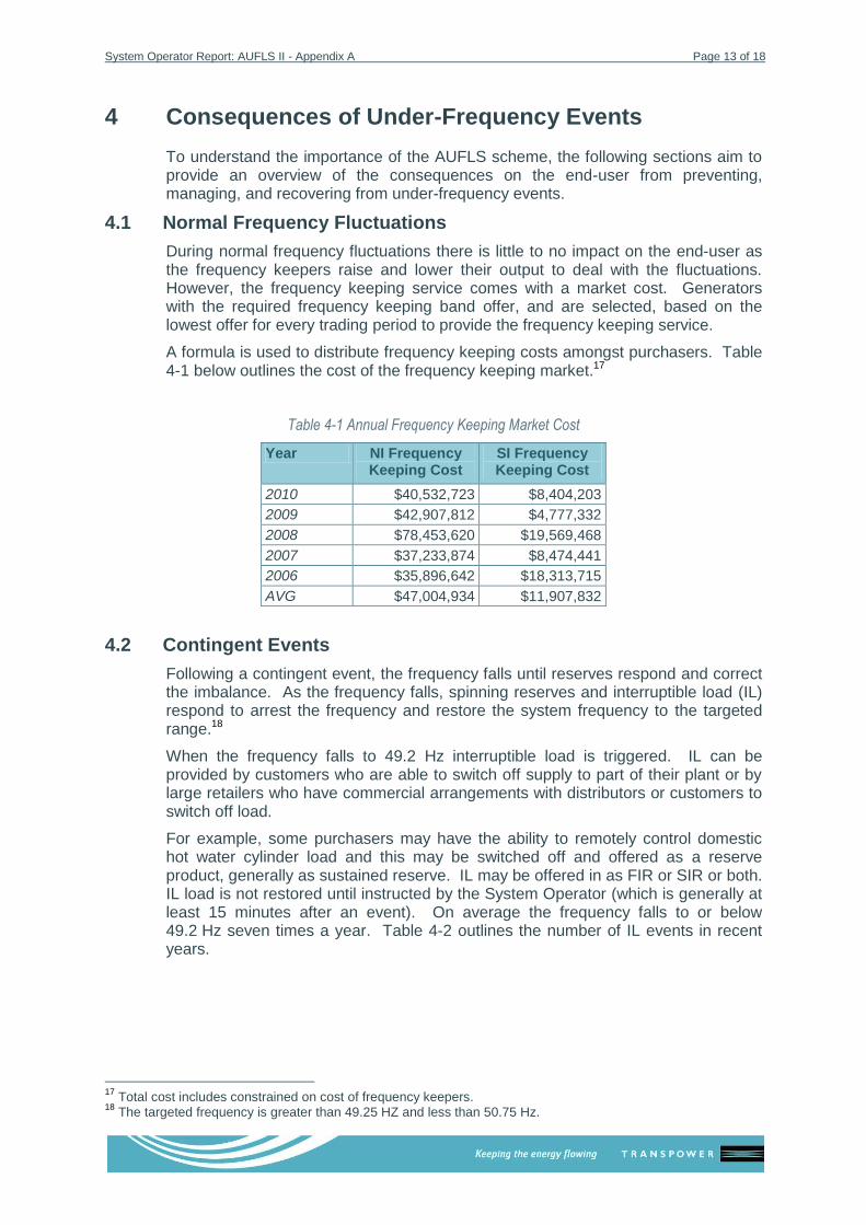
To understand the importance of the AUFLS scheme, the following sections aim to provide an overview of the consequences on the end-user from preventing, managing, and recovering from under-frequency events.

4.1 Normal Frequency Fluctuations

During normal frequency fluctuations there is little to no impact on the end-user as the frequency keepers raise and lower their output to deal with the fluctuations. However, the frequency keeping service comes with a market cost. Generators with the required frequency keeping band offer, and are selected, based on the lowest offer for every trading period to provide the frequency keeping service.

A formula is used to distribute frequency keeping costs amongst purchasers. Table 4-1 below outlines the cost of the frequency keeping market.17

Table 4-1 Annual Frequency Keeping Market Cost

Year NI Frequency Keeping Cost

SI Frequency Keeping Cost

2010 $40,532,723 $8,404,203

2009 $42,907,812 $4,777,332

2008 $78,453,620 $19,569,468

2007 $37,233,874 $8,474,441

2006 $35,896,642 $18,313,715

AVG $47,004,934 $11,907,832

4.2 Contingent Events

Following a contingent event, the frequency falls until reserves respond and correct the imbalance. As the frequency falls, spinning reserves and interruptible load (IL) respond to arrest the frequency and restore the system frequency to the targeted range.18

When the frequency falls to 49.2 Hz interruptible load is triggered. IL can be provided by customers who are able to switch off supply to part of their plant or by large retailers who have commercial arrangements with distributors or customers to switch off load.

For example, some purchasers may have the ability to remotely control domestic hot water cylinder load and this may be switched off and offered as a reserve product, generally as sustained reserve. IL may be offered in as FIR or SIR or both. IL load is not restored until instructed by the System Operator (which is generally at least 15 minutes after an event). On average the frequency falls to or below 49.2 Hz seven times a year. Table 4-2 outlines the number of IL events in recent years.

17

Total cost includes constrained on cost of frequency keepers. 18

The targeted frequency is greater than 49.25 HZ and less than 50.75 Hz.


Table 4-2 Annual Number of Interruptible Load Events19

Year Events

2010 9

2009 4

2008 7

2007 10

2006 3

2005 9

The impact on customers during an IL event is considered to be less than the price paid for the service as it is generally limited to hot water heating being shed or industrial process being interrupted. As this is an offered service the impact is generally well planned and managed by the IL provider. The market cost of purchasing these preventive measures is outlined in Table 4-3.

Table 4-3 Total Instantaneous Reserve cost for North and South Island

Year IL Cost Spinning Reserves

Total Reserves

201020

$8,902,126 $12,996,725 $22,082,532

2009 $28,397,552 $36,880,454 $65,278,006

2008 $24,657,007 $46,898,335 $71,555,342

2007 $8,589,463 $12,410,883 $21,000,347

2006 $11,912,913 $21,973,447 $33,886,360

AVG $16,491,812 $26,231,969 $42,760,517

4.3 Large Rare System Events

Following a large system event, the frequency can fall below 48 Hz. If the frequency continues to fall, the AUFLS blocks will be triggered and at least 16 % of customers will be disconnected from the system. If the frequency continues to fall then at least 32 % of customers will be disconnected from the system.21

Ideally most of the AUFLS load is intended to be made up of non-critical load with a low cost of interrupting such as residential customers and some commercial loads. Critical load, on the other hand, includes hospitals and other emergency services (i.e. fire stations, police stations, etc).

In some regions the size and configuration of the distribution networks does not allow for the ability to discriminate critical load from AUFLS blocks. In these cases hospitals and other emergency services may be included as part of an AUFLS block. Currently it assumed that major critical services have emergency backup power but the tripping of critical load on AUFLS feeders is less than ideal.22

19

Table was created from Under Frequency Event Database (UFED). Frequency events listed in the table are events where the frequency was at 49.2 or below.

20

In 2010 the „Total Reserves‟ column includes constrained on cost which are not accounted for as spinning reserves.

21 The percentage of load shed varies during different times of the day and year. Distributors are required to

provide a minimum of 32% of their load however at different times it may be much higher. 22

The System Operator is planning further investigation into the status and quantity of critical services connected to AUFLS feeders.


Generally, emergency backup power is limited to ensuring safety but does not guarantee continued operation.

After AUFLS load has been shed there are a number of factors that can affect the time to restore such load. Practical restoration time following an AUFLS event is likely to be between 90 minutes to up to 4 hours provided transmission assets and generation are available to restore the system.23 Given the variables that may exist at the time of an AUFLS event, it is important to note that the restoration times provide an informed estimate based on experience from power system events.

As referenced in the previous report, generally speaking, the System Operator can restore the system as fast as the distributors can connect the load, provided there is the transmission capacity and the generation available to support the load.

The current AUFLS arrangements are mandated and so there is minimal direct cost to the market except for the cost required for maintenance and testing. However if the AUFLS operate there is a cost of interruption which customers incur over time. This is known as the value of un-served energy or the Value of Lost Load (VoLL). As there are many discussions about estimating the cost of interruption, a sensitivity analysis was done and outlined in the following tables.

Table 4-4 NI AUFLS Block 1: Value of Lost Load for Single Event24

VoLL Est.

Restoration Time 2 hrs 4hrs 6hrs

$11.9/kWh $11,080,320 $22,160,640 $33,240,960

$23.8/kWh $22,160,640 $44,321,280 $66,481,920

$47.7/kWh $44,321,280 $88,642,560 $132,963,840

Table 4-5 NI AUFLS Total: Value of Lost Load for Single Event

VoLL Est.


$11.9/kWh $22,160,640 $44,321,280 $66,481,920

$23.8/kWh $44,321,280 $88,642,560 $132,963,840

$47.7/kWh $88,642,560 $177,285,120 $265,927,680

Table 4-6 SI AUFLS Block 1: Value of Lost Load for Single Event

VoLL Est.


$11.9/kWh $6,113,280 $12,226,560 $18,339,840

$23.8/kWh $12,226,560 $24,453,120 $36,679,680

$47.7/kWh $24,453,120 $48,906,240 $73,359,360

23

These restoration times provided are estimates based on experience of power system events. See the AUFLS technical report for further detail into restoration time of AUFLS.

24 All restoration time calculations assume a NI load of 2900 MW and SI load of 1600 MW, exemptions are not

included, and all load is assumed to be restored at the same time.


Table 4-7 SI AUFLS Block 1 and 2 Total: Value of Lost Load for Single Event

VoLL Est.


$11.9/kWh $12,226,560 $24,453,120 $36,679,680

$23.8/kWh $24,453,120 $48,906,240 $73,359,360

$47.7/kWh $48,906,240 $97,812,480 $146,718,720

4.4 System Collapse

If the AUFLS scheme and reserves on the system are insufficient to arrest the falling frequency, this will lead to cascade failure and system collapse or potentially fragmented with small generation electrical islands remaining.

In the event that the power system experiences a major disturbance that results in a black out, blackstart services would be required to start the restoration process of the power system. This is a complex process and at minimum will take 12 hours. It is considered much more likely to take longer than 24 hours to restore the system following a black out (possibly several days to achieve full restoration of the system).25

A loss of electricity over an extended period of time would have both significant and wide-ranging social and economic impacts on the end-user. The electricity system is the principal foundation for the restoration of other critical facilities and lifeline services. The impact of an extended outage needs to be carefully considered when reviewing the current AUFLS system.

A rough interruption cost estimate26 is used to estimate the cost of a blackout; the results are outlined in table A & B.

Table 4-8 NI Blackout Event Cost Estimate

VoLL Est.


$11.9/kWh $415,512,000 $831,024,000 $2,493,072,000

$23.8/kWh $831,024,000 $1,662,048,000 $4,986,144,000

$47.7/kWh $1,662,048,000 $3,324,096,000 $9,972,288,000

Table 4-9 SI Blackout Event Cost Estimate

VoLL Est.


$11.9/kWh $229,248,000 $458,496,000 $1,375,488,000

$23.8/kWh $458,496,000 $916,992,000 $2,750,976,000

$47.7/kWh $916,992,000 $1,833,984,000 $5,501,952,000

25

Black out restoration times are based on the findings of black start desk simulations. 26

The cost estimate used assumes all load will be fully restored in the specified time and then multiplied by the VoLL amount. This however is simplistic as load will be continually brought on until full restoration is reached. The figures above are only used as a crude estimate and not for any cost benefit analysis.


The blackstart service does incur a market cost some of which is born by the end-user. Half of the costs of the blackstart service are allocated to off-take customers and half are allocated generators.

Table 4-10 Total blackstart cost for the North and South Island

Year NI Blackstart

SI Blackstart

2010 $236,322 $268,649

2009 $189,074 $212,053

2008 $196,146 $204,896

2007 $187,687 $223,503

2006 $125,500 $199,200

AVG $186,946 $221,660


4.5 Overview of Consequences

Frequency (Hz) 50.2 50 49.8 49.5 49.2 NI 47.8/SI 47.5 NI 47.5/SI 45.5 NI 47/SI 45 Blackout

System Impact Spinng reserves

begin to

respond

IL trips AUFLS block 1

trips

AUFLS block 2

trips

Gen armed to

trip. Approx

25% of NI and

most SI Gen.

System

Collapse

Lights out

Customer Impact

What the customer

sees

Nil to minimal

Hot water

heating is cut.

Interruption to

some industrial

processes.

Up to 20% of

voluntary

demand shed.

Minimum 16%

of demand is

shed.

Power outage

for 16% of

customers

Minimum 32%

of demand is

shed .

Power outage

for 32% of

customers

Civil Emergency

Significant

social,

economic, &

environmental

consequences

Load Restoration Time N/A 15 mins 2 - 6 hrs 2 - 6 hrs 24 - 72 + hrs

Market (annual ) $26.2m $16.4m N/A N/A N/A $408,000

Value of Lost Load

(VoLL)*for a s ingle event***

N/A NI $460,000** NI $44m/SI $24m NI $1.6B/SI

$916m after 24

hours.

Impact on GDP

* Assumes a VoLL of $23,880/MWh

** Assumed an IL VoLL of $5,970/MWh

*** Assumes average island load of NI 2900 MW and SI 1600, AUFLS exemptions not considered, and AUFLS restoration time of 4hrs

Normal band

New Zealand

NI $44m/SI $24m

for block 2

NI $88m/SI $48m

for both blocks

N/A

Nil

Nil

Nil

N/A

$58.9m

N/A

Contingent Event Band AUFLS Band Cascade Failure Band

AUFLS II - Appendix A - Transpower New Zealand · It is important that the frequency remains close...

Documents

Transcript of AUFLS II - Appendix A - Transpower New Zealand · It is important that the frequency remains close...