Audio-visual Speech Processing - Cornell...
277
Audio-visual Speech Processing by Simon Lucey, BEng(Hons) PhD Thesis Submitted in Fulfilment of the Requirements for the Degree of Doctor of Philosophy at the Queensland University of Technology Speech Research Laboratory School of Electrical & Electronic Systems Engineering April 2002
Transcript of Audio-visual Speech Processing - Cornell...
Audio-visual Speech Processing
by
Simon Lucey, BEng(Hons)
PhD Thesis
Submitted in Fulfilment
of the Requirements
for the Degree of
Doctor of Philosophy
at the
Queensland University of Technology
Speech Research Laboratory
School of Electrical & Electronic Systems Engineering
April 2002


Substitute the “official” thesissignature page here.


Keywords
Audio-visual speech processing, speaker identification, speaker verification, speech
recognition, classifier combination, facial feature detection, pattern recognition

Abstract
Speech is inherently bimodal, relying on cues from the acoustic and visual speech
modalities for perception. The McGurk effect demonstrates that when humans
are presented with conflicting acoustic and visual stimuli, the perceived sound
may not exist in either modality. This effect has formed the basis for modelling
the complementary nature of acoustic and visual speech by encapsulating them
into the relatively new research field of audio-visual speech processing (AVSP).
Traditional acoustic based speech processing systems have attained a high level
of performance in recent years, but the performance of these systems is heavily
dependent on a match between training and testing conditions. In the presence
of mismatched conditions (eg. acoustic noise) the performance of acoustic speech
processing applications can degrade markedly. AVSP aims to increase the robust-
ness and performance of conventional speech processing applications through the
integration of the acoustic and visual modalities of speech, in particular the tasks
of isolated word speech and text-dependent speaker recognition.
Two major problems in AVSP are addressed in this thesis, the first of which
concerns the extraction of pertinent visual features for effective speech reading
and visual speaker recognition. Appropriate representations of the mouth are ex-
plored for improved classification performance for speech and speaker recognition.
Secondly, there is the question of how to effectively integrate the acoustic and
visual speech modalities for robust and improved performance. This question is
explored in-depth using hidden Markov model (HMM) classifiers. The develop-

ii
ment and investigation of integration strategies for AVSP required research into
a new branch of pattern recognition known as classifier combination theory. In
this thesis a novel framework is presented for optimally combining classifiers so
their combined performance is greater than any of those classifiers individually.
The benefits of this framework are not restricted to AVSP, as they can be applied
to any task where there is a need for combining independent classifiers.
Contents
Abstract i
List of Tables xi
List of Figures xiii
Notation xix
Acronyms & Abbreviations xxi
Certification of Thesis xxv
Acknowledgments xxvii
Chapter 1 Introduction 1
1.1 Motivation and Overview . . . . . . . . . . . . . . . . . . . . . . . 1
1.1.1 Measuring Speech Recognition Performance . . . . . . . . 3
1.1.2 Measuring Speaker Recognition Performance . . . . . . . . 4
iv CONTENTS
1.1.3 Audio-visual Database . . . . . . . . . . . . . . . . . . . . 5
1.2 Aims and Objectives . . . . . . . . . . . . . . . . . . . . . . . . . 5
1.3 Outline of Thesis . . . . . . . . . . . . . . . . . . . . . . . . . . . 6
1.4 Original Contributions of Thesis . . . . . . . . . . . . . . . . . . . 9
1.5 Publications resulting from research . . . . . . . . . . . . . . . . . 11
1.5.1 International Journal Publications . . . . . . . . . . . . . . 11
1.5.2 International Conference Publications . . . . . . . . . . . . 12
Chapter 2 Audio-visual Speech Processing 15
2.1 Introduction . . . . . . . . . . . . . . . . . . . . . . . . . . . . . . 15
2.2 Phonetics of Visual Speech . . . . . . . . . . . . . . . . . . . . . . 16
2.3 Speech Production . . . . . . . . . . . . . . . . . . . . . . . . . . 17
2.4 Speech Reading . . . . . . . . . . . . . . . . . . . . . . . . . . . . 19
2.5 Audio-visual Integration . . . . . . . . . . . . . . . . . . . . . . . 20
2.6 Visual Speaker Dependencies . . . . . . . . . . . . . . . . . . . . . 24
2.7 Speech Enhancement and Coding . . . . . . . . . . . . . . . . . . 24
2.8 Chapter Summary . . . . . . . . . . . . . . . . . . . . . . . . . . 26
Chapter 3 Classifier theory 29
3.1 Introduction . . . . . . . . . . . . . . . . . . . . . . . . . . . . . . 29
CONTENTS v
3.2 Classifier Theory Background . . . . . . . . . . . . . . . . . . . . 30
3.3 Non-parametric Classifiers . . . . . . . . . . . . . . . . . . . . . . 31
3.4 Discriminant Classifiers . . . . . . . . . . . . . . . . . . . . . . . . 32
3.5 Parametric Classifiers . . . . . . . . . . . . . . . . . . . . . . . . . 34
3.5.1 Maximum likelihood estimation . . . . . . . . . . . . . . . 35
3.5.2 Expectation maximisation algorithm . . . . . . . . . . . . 36
3.6 Gaussian Mixture Models . . . . . . . . . . . . . . . . . . . . . . 37
3.6.1 Classifier complexity versus training set size . . . . . . . . 38
3.6.2 GMM parameter estimation . . . . . . . . . . . . . . . . . 40
3.6.3 GMM initialisation . . . . . . . . . . . . . . . . . . . . . . 40
3.7 Hidden Markov Models . . . . . . . . . . . . . . . . . . . . . . . . 41
3.7.1 Hidden states . . . . . . . . . . . . . . . . . . . . . . . . . 43
3.7.2 Viterbi decoding algorithm . . . . . . . . . . . . . . . . . . 45
3.7.3 HMM parameter estimation . . . . . . . . . . . . . . . . . 46
3.8 Chapter Summary . . . . . . . . . . . . . . . . . . . . . . . . . . 51
Chapter 4 Facial Feature Detection for AVSP 53
4.1 Introduction . . . . . . . . . . . . . . . . . . . . . . . . . . . . . . 53
4.2 Front-end Effect . . . . . . . . . . . . . . . . . . . . . . . . . . . . 55
vi CONTENTS
4.3 Restricted Scope for AVSP . . . . . . . . . . . . . . . . . . . . . . 56
4.3.1 Validation . . . . . . . . . . . . . . . . . . . . . . . . . . . 58
4.4 Defining the Face Search Area . . . . . . . . . . . . . . . . . . . . 60
4.5 Paradigms for Object Detection/Location . . . . . . . . . . . . . 63
4.6 Chapter Summary . . . . . . . . . . . . . . . . . . . . . . . . . . 68
Chapter 5 Appearance Based Detection 69
5.1 Introduction . . . . . . . . . . . . . . . . . . . . . . . . . . . . . . 69
5.1.1 Appearance based detection framework . . . . . . . . . . . 70
5.1.2 Principal component analysis . . . . . . . . . . . . . . . . 72
5.1.3 Linear discriminant analysis . . . . . . . . . . . . . . . . . 75
5.1.4 Single class detection . . . . . . . . . . . . . . . . . . . . . 77
5.1.5 Two class detection . . . . . . . . . . . . . . . . . . . . . . 82
5.1.6 Evaluation of appearance models . . . . . . . . . . . . . . 85
5.2 Chapter Summary . . . . . . . . . . . . . . . . . . . . . . . . . . 90
Chapter 6 Feature Invariant Lip Location/Tracking 91
6.1 Introduction . . . . . . . . . . . . . . . . . . . . . . . . . . . . . . 91
6.2 Lip Segmentation . . . . . . . . . . . . . . . . . . . . . . . . . . . 93
6.2.1 Formulation of segmentation problem . . . . . . . . . . . . 94
CONTENTS vii
6.2.2 Chromatic representations of the lips . . . . . . . . . . . . 95
6.3 Validating Segmentation Performance . . . . . . . . . . . . . . . . 96
6.4 Supervised Lip Segmentation . . . . . . . . . . . . . . . . . . . . 97
6.5 Unsupervised Lip Segmentation . . . . . . . . . . . . . . . . . . . 101
6.5.1 Clustering results . . . . . . . . . . . . . . . . . . . . . . . 102
6.6 Lip Contour Fitting . . . . . . . . . . . . . . . . . . . . . . . . . . 104
6.7 Point Distribution Models and Potential Images . . . . . . . . . . 106
6.8 Edge Maps and Potential Force Fields . . . . . . . . . . . . . . . 107
6.9 Gradient Vector Flow . . . . . . . . . . . . . . . . . . . . . . . . . 109
6.9.1 Numerical implementation of creating GVF field . . . . . . 110
6.10 Calculating Movement for each Model Point . . . . . . . . . . . . 111
6.11 Performance of Lip Location Algorithm . . . . . . . . . . . . . . . 113
6.12 Chapter Summary . . . . . . . . . . . . . . . . . . . . . . . . . . 114
Chapter 7 Feature Extraction 117
7.1 Introduction . . . . . . . . . . . . . . . . . . . . . . . . . . . . . . 117
7.2 Acoustic Speech Features . . . . . . . . . . . . . . . . . . . . . . . 118
7.2.1 Linear prediction analysis . . . . . . . . . . . . . . . . . . 120
7.2.2 Filter bank analysis . . . . . . . . . . . . . . . . . . . . . . 121
viii CONTENTS
7.2.3 Improving robustness to acoustic train/test
mismatches . . . . . . . . . . . . . . . . . . . . . . . . . . 122
7.3 Visual Speech Features . . . . . . . . . . . . . . . . . . . . . . . . 124
7.3.1 Area based representations . . . . . . . . . . . . . . . . . . 125
7.3.2 Contour based representations . . . . . . . . . . . . . . . . 127
7.3.3 Area vs. contour features . . . . . . . . . . . . . . . . . . . 128
7.4 Delta Features . . . . . . . . . . . . . . . . . . . . . . . . . . . . . 130
7.5 Evaluation of Speech Features . . . . . . . . . . . . . . . . . . . . 131
7.5.1 Training of hidden Markov models . . . . . . . . . . . . . 133
7.5.2 Speech recognition performance . . . . . . . . . . . . . . . 134
7.5.3 Speaker recognition performance . . . . . . . . . . . . . . 137
7.6 Chapter Summary . . . . . . . . . . . . . . . . . . . . . . . . . . 138
Chapter 8 Independent Classifier Combination Theory 141
8.1 Introduction . . . . . . . . . . . . . . . . . . . . . . . . . . . . . . 141
8.2 Bounds for Independent Classifier Combination . . . . . . . . . . 144
8.3 Exaptation vs. Adaptation . . . . . . . . . . . . . . . . . . . . . . 146
8.4 Modelling Train/Test Mismatches . . . . . . . . . . . . . . . . . . 147
8.5 Form of Mismatch Likelihood and Priors . . . . . . . . . . . . . . 149
8.5.1 Synthetic example . . . . . . . . . . . . . . . . . . . . . . 151
CONTENTS ix
8.5.2 Empirical validation . . . . . . . . . . . . . . . . . . . . . 152
8.6 Combination Strategies . . . . . . . . . . . . . . . . . . . . . . . . 155
8.6.1 Sum rule . . . . . . . . . . . . . . . . . . . . . . . . . . . . 155
8.6.2 Other combination strategies . . . . . . . . . . . . . . . . . 158
8.6.3 Weighted product rule . . . . . . . . . . . . . . . . . . . . 160
8.6.4 Weighted sum rule . . . . . . . . . . . . . . . . . . . . . . 164
8.6.5 An elucidative example . . . . . . . . . . . . . . . . . . . . 167
8.6.6 Adaptation through the weighted product rule . . . . . . . 171
8.7 Exaptation or Adaptation, a Paradox? . . . . . . . . . . . . . . . 176
8.8 Defining a Critical Region of Knowledge . . . . . . . . . . . . . . 177
8.9 Chapter Summary . . . . . . . . . . . . . . . . . . . . . . . . . . 181
Chapter 9 Integration Strategies for Audio-visual Speech Process-
ing 183
9.1 Introduction . . . . . . . . . . . . . . . . . . . . . . . . . . . . . . 183
9.2 Integration Background and Scope . . . . . . . . . . . . . . . . . 184
9.3 Hidden Markov Models, Training and Integration Strategies . . . 188
9.3.1 Multistream HMMs . . . . . . . . . . . . . . . . . . . . . . 191
9.3.2 The equivalence of MI and LI . . . . . . . . . . . . . . . . 195
9.3.3 LI combination strategies . . . . . . . . . . . . . . . . . . 198
x CONTENTS
9.3.4 Calculating a suitable α . . . . . . . . . . . . . . . . . . . 200
9.3.5 Sensitivity of combination strategies to α . . . . . . . . . . 207
9.3.6 A hybrid between product and sum rules . . . . . . . . . . 208
9.4 Results and Discussion . . . . . . . . . . . . . . . . . . . . . . . . 209
9.4.1 Case I . . . . . . . . . . . . . . . . . . . . . . . . . . . . . 210
9.4.2 Case II . . . . . . . . . . . . . . . . . . . . . . . . . . . . . 215
9.5 Chapter Summary . . . . . . . . . . . . . . . . . . . . . . . . . . 216
Chapter 10 Conclusions and Future Work 219
10.1 Conclusions . . . . . . . . . . . . . . . . . . . . . . . . . . . . . . 219
10.2 Future Work . . . . . . . . . . . . . . . . . . . . . . . . . . . . . . 222
Bibliography 225
Appendix A Gaussian Identities in Unmatched Conditions 238
A.1 The Effect of Scale Train/Test Mismatch . . . . . . . . . . . . . . 239

List of Tables
6.1 Average error rates for different GMM classifier topologies and
chromatic features. . . . . . . . . . . . . . . . . . . . . . . . . . . 98
6.2 Average error rates for unsupervised clustering using single clusters
for the mouth and background classes across various chromatic
features. . . . . . . . . . . . . . . . . . . . . . . . . . . . . . . . . 103
7.1 WER rates for train and test sets on the M2VTS database (note
best performing visual features have been highlighted). . . . . . . 135
7.2 SER for train and test sets on the M2VTS database (note best
performing visual features have been highlighted). . . . . . . . . . 137
9.1 Case I : Word error rates (WER) for integration strategies under
clean conditions using optimal α∗ (best strategies are highlighted). 212
9.2 Case I: Word error rates (WER) comparing asynchronous and syn-
chronous multistream HMM topologies when the audio classifier
has a train/test mismatch from acoustic noise (20 dB). The op-
timal weighting factor α∗ was found for both strategies using an
exhaustive search. . . . . . . . . . . . . . . . . . . . . . . . . . . . 212

xii LIST OF TABLES
9.3 Case I: Equal error rates (EER) and speaker error rates (SER)
for integration strategies under clean conditions using optimal α∗
(best strategies are highlighted for verification and identification). 213
9.4 2-D state histograms taken from M2VTS verification set for digits
(a) FIVE and (b) EIGHT. . . . . . . . . . . . . . . . . . . . . . . 213

List of Figures
2.1 Schematic representation of the complete physiological mechanism
of speech production highlighting the externally visible area.(adapted
from Rabiner and Juang [1] pg. 17) . . . . . . . . . . . . . . . . . 18
3.1 Discrete states in a Markov model are represented by nodes and,
the transition probabilities by links. . . . . . . . . . . . . . . . . . 42
4.1 Graphical depiction of overall detection/location/tracking frontend
to an AVSP application. . . . . . . . . . . . . . . . . . . . . . . . 55
4.2 Graphical depiction of the cascading front end effect. . . . . . . . 55
4.3 Relations between expected eye (cl, cr) and mouth (cm) positions
their estimated ones. . . . . . . . . . . . . . . . . . . . . . . . . . 59
4.4 Example of how the mouth position cm is found from the bisection
of the left and right corners of the mouth. . . . . . . . . . . . . . 60
4.5 Example of bounding boxes used to gather skin and background
training observations . . . . . . . . . . . . . . . . . . . . . . . . . 63
4.6 Original example faces taken from M2VTS database to be used for
face segmentation. . . . . . . . . . . . . . . . . . . . . . . . . . . 64

xiv LIST OF FIGURES
4.7 Binary potential maps generated using chromatic skin and back-
ground models. . . . . . . . . . . . . . . . . . . . . . . . . . . . . 65
5.1 Demonstration of how contents of window W (x, y) can be repre-
sented as vector yt. . . . . . . . . . . . . . . . . . . . . . . . . . . 70
5.2 Example of how intra-class clustering can improve LDA perfor-
mance. (a) Multimodal scenario of where LDA does not work for
2 class problem due to no mean separation. (b) Reformulating the
same problem with 4 classes allows for mean separation. . . . . . 77
5.3 Example of multi-modal clustering of mouth sub-images within
principal sub-space. . . . . . . . . . . . . . . . . . . . . . . . . . . 81
5.4 Example of (a) mouth sub-images (b) mouth background sub-images. 83
5.5 Example of (a) eye sub-images (b) eye background sub-images. . . 84
5.6 DET curve of different detection metrics for separation between
eye and background sub-images. . . . . . . . . . . . . . . . . . . . 87
5.7 DET curve of different detection metrics for separation between
mouth and background sub-images. . . . . . . . . . . . . . . . . . 88
5.8 Depiction of how skin map is divided to search for facial features. 89
6.1 Supervised segmentation error rates across the 36 speakers of the
M2VTS database. . . . . . . . . . . . . . . . . . . . . . . . . . . . 99
6.2 Segmented images across some subjects of the M2VTS database
through supervised segmentation. . . . . . . . . . . . . . . . . . . 100

LIST OF FIGURES xv
6.3 Unsupervised segmentation error rates across the 36 speakers of
the M2VTS database. . . . . . . . . . . . . . . . . . . . . . . . . 104
6.4 Segmented images across some subjects of the M2VTS database
through unsupervised segmentation. . . . . . . . . . . . . . . . . . 105
6.5 Demonstration of how potential image is created. . . . . . . . . . 106
6.6 Process of calculating normalised GVF force field. . . . . . . . . . 110
6.7 Demonstration of robust contour fitting on a potential image with
unwanted lip pixel artifacts. . . . . . . . . . . . . . . . . . . . . . 114
6.8 Demonstration of contour fitting on potential image with missing
lip pixels. . . . . . . . . . . . . . . . . . . . . . . . . . . . . . . . 115
8.1 Venn diagram of changes in train/test conditions, (a) Stst ⊆ Strn
(similar train/test conditions), (b) Stst * Strn (different train/test
conditions). . . . . . . . . . . . . . . . . . . . . . . . . . . . . . . 148
8.2 Depiction of synthetic example class models. 90% ellipsoid bound-
aries shown for both classes and contexts. . . . . . . . . . . . . . 152
8.3 Empirical results for synthetic example. . . . . . . . . . . . . . . . 153
8.4 Empirical results for synthetic example with unequal priors. . . . 155
8.5 Graphical depiction of the p(o|Ω) and p(o|Ω) density functions.
Note p(o|Ω) is a mixture of N = 5 classes in this depiction. . . . . 168
8.6 Error rates for various combination strategies for synthetic example.170

xvi LIST OF FIGURES
8.7 Depiction of how empirical error rates for the synthetic example
have the weighted sum and weighted product rules lying between
the ideal product and catastrophic fusion error bounds. . . . . . . 171
8.8 Comparison of optimal weightings for weighted sum Fwsr() and
weighted product Fwpr() rules for synthetic example. . . . . . . . 172
8.9 Homoscedastic variances of MFCCs taken from the M2VTS database
across varying amounts of additive white Gaussian noise. . . . . . 175
8.10 Examples of two different qualitative types of train/test mismatches.
(a) Translational mismatch (b) Scale mismatch. . . . . . . . . . . 179
9.1 Depiction of possible levels of integration. . . . . . . . . . . . . . 185
9.2 Example of 2D left to right HMM state lattice for asynchronous
and synchronous decoding. . . . . . . . . . . . . . . . . . . . . . . 192
9.3 Effect of varying weighting factor α for two different acoustic noise
contexts (i.e. Clean and 0dB) for (a) speaker recognition and (b)
speech recognition. . . . . . . . . . . . . . . . . . . . . . . . . . . 201
9.4 Comparing the log-likelihood approximations of βa using audio log-
likelihoods taken from the speech and speaker recognition HMM
classifiers. . . . . . . . . . . . . . . . . . . . . . . . . . . . . . . . 204
9.5 Evaluation of techniques for approximating α∗ in (a) speech recog-
nition and (b) speaker recognition using the weighted product rule. 206

9.6 Comparison between narrowly tuned and broadly tuned α∗ weight-
ings for the task of (a) speech recognition and (b) speaker recog-
nition, across varying amounts of additive acoustic noise. (Note
the α∗ weighting for the broad context was optimised for a clean
(i.e. 40 dB) audio noise context.) . . . . . . . . . . . . . . . . . . 207
9.7 Case I : DET curves various integration strategies under clean con-
ditions. . . . . . . . . . . . . . . . . . . . . . . . . . . . . . . . . . 211
9.8 Case II: Word error rates (WER) for various LI strategies over a
broad audio noise context. . . . . . . . . . . . . . . . . . . . . . . 214
9.9 Case II: Subject error rates (SER) for various LI strategies over a
broad audio noise context. . . . . . . . . . . . . . . . . . . . . . . 215
9.10 Case II: Equal error rates (EER) for various LI strategies for a
broad audio noise context. . . . . . . . . . . . . . . . . . . . . . . 216

xviii LIST OF FIGURES

Notation
tr(A) =∑N
i=1 λi, the trace of matrix A where λi are the eigenvalues of matrix A.
det(A) =∏N
i=1 λi, the determinant of matrix A where λi are the eigenvalues of
matrix A.
A(N×M) is a matrix A with dimensions N ×M .
a′ is the transpose of vector a, note all vectors are column vectors.
N (µ,Σ) is the multivariate normal (Gaussian) distribution with mean µ and
covariance matrix Σ. The same Gaussian, evaluated at the point o, is
denoted as N (µ,Σ)|o.
∼ refers to being distributed according to, for example o ∼ p(o) or S ∼ p(o).
p(o|ωi) is the conditional likelihood function for class ωi and observation vector o.
Pr(ωi|o) is the a posteriori conditional class probability for class ωi and obser-
vation o.
P (ωi) is the a priori class probability for class ωi.
Ed the expectation of the random variable d.
V ard the variance of the random variable d.
Ed is the sample expectation of the individual elements of the vector d.
V ard is the sample variance of the individual elements of the vector d.


Acronyms & Abbreviations
AAM Active appearance model
ANN Artificial neural network
ASM Active shape models
AVSP Audio-visual speech processing
CMS Cepstral mean subtraction
DCT Discrete cosine transform
DET Detection error tradeoff
DS Discriminant space
EER Equal error rate
EI Early integration
EM Expectation-maximization
FA False acceptance
FFD Facial feature detection
FR False rejection
GMM Gaussian mixture model
GPV Grand profile vector

xxii LIST OF FIGURES
GVF Gradient vector flow
HMM Hidden Markov model
LDA Linear discriminant analysis
LI Late integration
LPC Linear predictive coefficient
M2VTS Multimodal verification for teleservices and security applications
MAHMM Multi-stream asynchronous hidden Markov model
MFCC Mel-Frequency cepstral coefficients
MI Middle integration
ML Maximum likelihood
MLP Multi-layer perceptron
MRF Markov random field
MRPCA Mean-removed principal component analysis
MSE Mean square error
MSHMM Multi-stream synchronous hidden Markov model
OS Object space
PCA Principal component analysis
PDM Point distribution model
ROI Region of interest
RS Residual space
SER Speaker error rate
SH State histogram

LIST OF FIGURES xxiii
SLDA Speaker linear discriminant analysis
SNR Signal to noise ratio
VQ Vector quantization
WER Word error rate
WLDA Word linear discriminant analysis


Certification of Thesis
The work contained in this thesis has not been previously submitted for a degree
or diploma at any other higher educational institution. To the best of my knowl-
edge and belief, the thesis contains no material previously published or written
by another person except where due reference is made.
Signed:
Date:

xxvi LIST OF FIGURES
Acknowledgments
It is not possible to thank everybody who has had an involvement with me dur-
ing the course of Ph.D. However, there are some people who must be thanked.
Firstly, I would like to thank my parents whose undying support and unwavering
encouragement has helped me achieve beyond my greatest expectations. Their
insights, laughter and guidance has aided me far more in this stage of my life
than they will ever know.
I would also like to thank my principal supervisor Prof. Sridha Sridharan for
his guidance and encouragement throughout my course of study. The research
environment he has created at the speech laboratory, as well as the opportunities
to visit foreign institutions and international conferences, is testimony to his
commitment to excellence in research and development, and for that I am very
thankful.
I must also thank my associate supervisors Dr. Vinod Chandran and Prof. Miles
Moody for their assistance throughout the project along with their many valuable
suggestions and improvements for the thesis. In particular I would like to thank
Vinod for his conscientious reviewing of my conference and journal papers as
well as my thesis draft, his diligence in this area has helped me become a better
researcher. A thankyou must be extended to Dr. John Leis, who first placed trust
in my ability and gave me the initial opportunity to join the Speech Laboratory.
I was fortunate, during the course of my research, to spend three months re-

xxviii ACKNOWLEDGMENTS
searching at Carnegie Mellon University under the tutelage of A/Prof. Tsuhan
Chen. This was an invaluable experience obviously from the perspective of vis-
iting such a prestigious institution, but the manner and professionalism of the
staff and students there has also had a profound effect on me. Their hunger for
scientific truth and their search for a fundamental understanding to the problems
we deal with, has changed my ideals on research forever.
The past and present members of the Speech Laboratory must also be acknowl-
edged, the jovial atmosphere created by the lads and their expertise in research
has made it a pleasure to be their colleague and, more importantly, their friend.
John Dines and Jason Pelecanos have been of particular help to me during the
latter stage of my Ph.D., both boys have acted as a sounding board for my own
bizarre form of logic and have been essential to the completion of the thesis.
Iain McCowan, Tim Wark, Michael Mason, Andrew Busch, David Cole, Darren
Moore, Darren Butler, Anthony Ngyuen and Eddie Wong all deserve special men-
tion for their input at various times. Although, between us all, we still have not
been able to divulge the mysterious inner workings of the McCowan constant.
A final acknowledgement must go to all my family (Patty, Owen and Jedrow
I haven’t forgotten you) and friends who have put up with me over the years.
Hopefully all your tolerance has not been in vain.
Simon Lucey
Queensland University of Technology
April 2002
Chapter 1
Introduction
1.1 Motivation and Overview
Speech production and perception is inherently bimodal. Of late there has been
increased interest in using the visual modality in combination with the normally
used acoustic modality for improved speech processing. This field of study has
gained the title of audio-visual speech processing (AVSP). Traditional acoustic
based speech processing systems have attained a high level of performance in re-
cent years, but the performance of these systems is heavily dependent on a match
between train and test conditions. In the presence of mismatched conditions (i.e.
acoustic noise) the performance of acoustic speech processing applications can
degrade markedly. The visual speech modality is independent to most possible
degradations in the acoustic modality. This independence, along with the bi-
modal nature of speech, naturally allows the visual speech modality to act in a
complementary capacity to the acoustic speech modality. It is hoped that the
integration of these two speech modalities will aid in the creation of more robust
and effective speech processing applications in the future.
AVSP inherently requires the command of a broad gamut of skills in signal pro-
2 1.1 Motivation and Overview
cessing ranging from traditional speech and image processing to theoretical pat-
tern recognition theory. In many circumstances these fields of study overlap,
reinforce and contradict each other, all of which adds to the rich tapestry of
knowledge required for designing viable AVSP systems. Primarily there are two
points of interest associated with the design of an effective AVSP application.
1. Gaining of an appropriate representation of the visual speech modality.
2. The effective integration of the acoustic and visual speech modalities in the
presence of a variety of degradations.
The first point of interest concerns gaining a representation of the visual speech
modality that is suitable for additional post-processing (i.e. classification). This
problem encapsulates the difficult computer vision tasks of face detection, and
subsequent facial feature detection (i.e. eyes and mouth). After sufficient de-
tection and normalisation of the face, visual facial features pertinent to speech
(i.e. the mouth) must be parameterised in a manner that is conducive for effec-
tive post-processing. Visual feature extraction is a large problem still facing the
AVSP community and is addressed throughout this thesis.
The second point involves the interesting question of how best to combine the
acoustic and visual speech modalities. This problem delves into the very mechan-
ics of speech and gives insights into how we as humans integrate the acoustic and
visual modalities of speech. Classifier combination theory plays a very impor-
tant role in such integration. As with many pursuits, lessons learnt from AVSP
concerning classifier combination theory, can readily be applied to other pattern
recognition problems and have ramifications reaching farther than just speech
processing. Classifier combination theory aims to combine multiple classifiers in
such a manner that their combined performance is greater than any of the classi-
fiers individually. Serious inroads need to be made concerning the theory behind
AVSP integration, and more fundamentally classifier combination theory. Again
this thesis tries to address such issues.
1.1 Motivation and Overview 3
In this thesis the field of AVSP is largely constrained to the tasks of,
(i) speech recognition, and
(ii) text-dependent speaker recognition
Speech recognition systems are now available commercially for a variety of tasks,
such as voice dictation on computers and voice dialing on mobile phones, not to
mention a plethora of other applications. Automated speaker recognition systems
have immediate benefits in any application requiring security as required in the
banking sector and military, among others. Text dependent applications for the
task of speaker recognition typically out-perform their text independent counter
parts due to the simplification of the recognition task. Text-dependent refers to
the speaker having to say a set utterance for recognition, as opposed to text-
independent approaches which are largely invariant to the type of utterance. By
introducing the added robustness and performance improvement possible from
the visual speech modality, for the tasks of speech and speaker recognition, such
applications will hopefully enjoy increased performance in everyday situations.
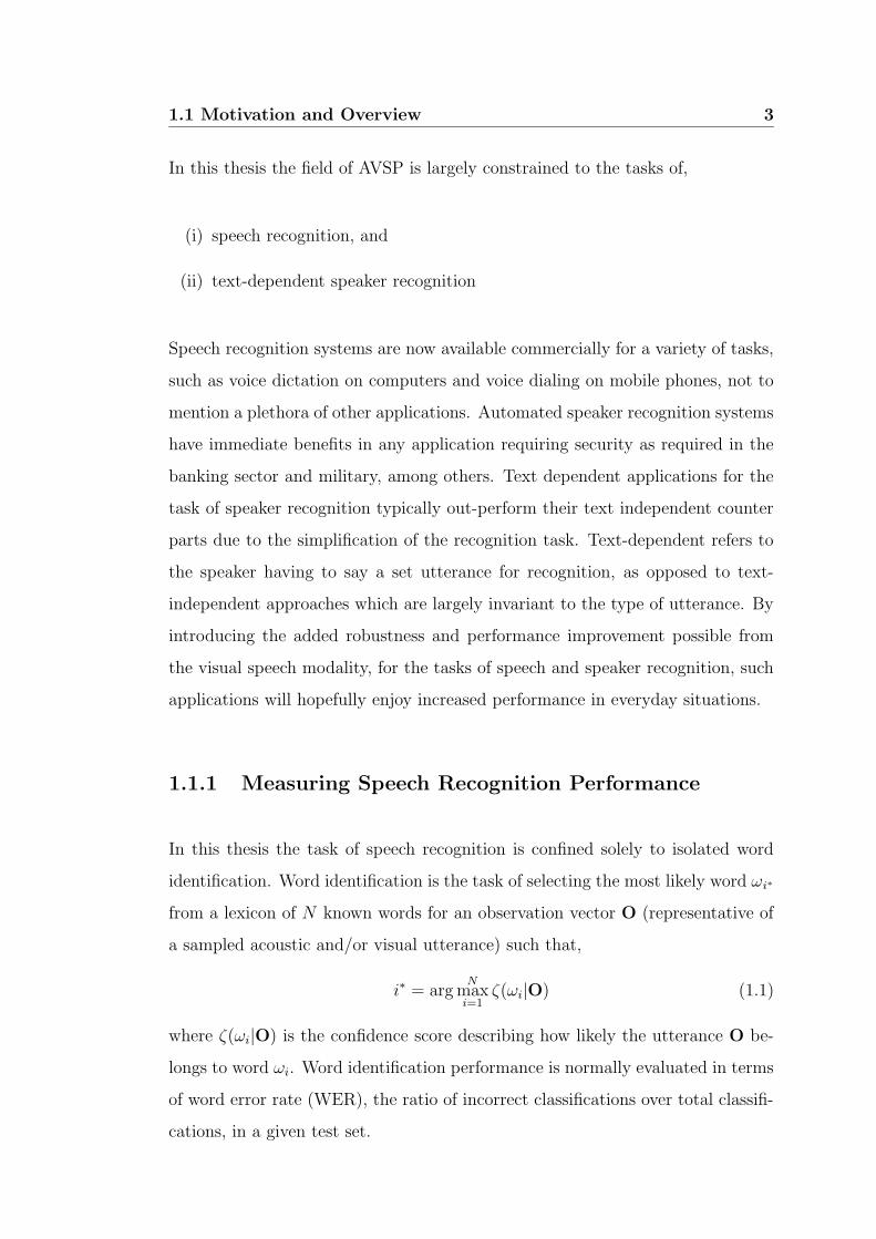
1.1.1 Measuring Speech Recognition Performance
In this thesis the task of speech recognition is confined solely to isolated word
identification. Word identification is the task of selecting the most likely word ωi∗
from a lexicon of N known words for an observation vector O (representative of
a sampled acoustic and/or visual utterance) such that,
i∗ = argN
maxi=1
ζ(ωi|O) (1.1)
where ζ(ωi|O) is the confidence score describing how likely the utterance O be-
longs to word ωi. Word identification performance is normally evaluated in terms
of word error rate (WER), the ratio of incorrect classifications over total classifi-
cations, in a given test set.
4 1.1 Motivation and Overview
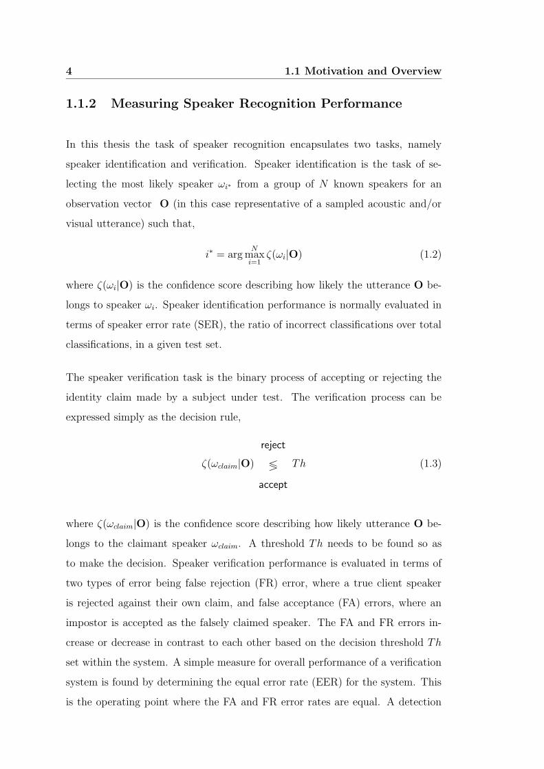
1.1.2 Measuring Speaker Recognition Performance
In this thesis the task of speaker recognition encapsulates two tasks, namely
speaker identification and verification. Speaker identification is the task of se-
lecting the most likely speaker ωi∗ from a group of N known speakers for an
observation vector O (in this case representative of a sampled acoustic and/or
visual utterance) such that,
i∗ = argN
maxi=1
ζ(ωi|O) (1.2)
where ζ(ωi|O) is the confidence score describing how likely the utterance O be-
longs to speaker ωi. Speaker identification performance is normally evaluated in
terms of speaker error rate (SER), the ratio of incorrect classifications over total
classifications, in a given test set.
The speaker verification task is the binary process of accepting or rejecting the
identity claim made by a subject under test. The verification process can be
expressed simply as the decision rule,
ζ(ωclaim|O)
reject
≶
accept
Th (1.3)
where ζ(ωclaim|O) is the confidence score describing how likely utterance O be-
longs to the claimant speaker ωclaim. A threshold Th needs to be found so as
to make the decision. Speaker verification performance is evaluated in terms of
two types of error being false rejection (FR) error, where a true client speaker
is rejected against their own claim, and false acceptance (FA) errors, where an
impostor is accepted as the falsely claimed speaker. The FA and FR errors in-
crease or decrease in contrast to each other based on the decision threshold Th
set within the system. A simple measure for overall performance of a verification
system is found by determining the equal error rate (EER) for the system. This
is the operating point where the FA and FR error rates are equal. A detection

1.2 Aims and Objectives 5
error tradeoff (DET) curve, similar to a receiver operating characteristic (ROC)
curve, can also be used to represent the trade off between the two errors for a
varying threshold.
1.1.3 Audio-visual Database
The M2VTS database [2] was used for experiments in this thesis. Out of the
possible 37 subjects in the database the subject ‘pm’ was excluded from testing,
due to his beard which was thought to unfairly skew the verification results.
This database has been used in previous AVSP work [3, 4, 5], and is typical
of conditions met in normal AVSP environments. The database was used for
experiments in this thesis concerning the tasks of facial feature detection, speech
and speaker detection. It consisted of, 36 subjects (male and female) speaking
four repetitions (shots) of ten French digits from zero to nine.
1.2 Aims and Objectives
Audio-visual speech processing is still in a relative state of infancy, with minimal
research having been conducted in many of its areas to date. In particular the
tasks of effective visual feature extraction, and the successful integration of the
acoustic and visual speech modalities across a gamut of train/test conditions,
have yet to be successfully addressed.
The general aims of this thesis are:
(i) To investigate, evaluate and develop techniques for face detection, and sub-
sequent facial feature detection for purposes of normalisation and visual
feature extraction.
(ii) Based on psychological, physiological, theoretical and empirical knowledge
6 1.3 Outline of Thesis
of human and machine speech perception evaluate and develop effective
strategies for integrating the acoustic and visual modalities of speech for
speech and speaker recognition.
(iii) Develop a framework for successful independent classifier combination, with
particular emphasis being placed on the task of AVSP.
The research objectives are:
(i) Review and evaluate the current state of research in AVSP for the specific
tasks of speech and speaker recognition.
(ii) Investigate and improve current techniques for face and facial feature de-
tection as an front-end to an AVSP system.
(iii) Evaluate current visual feature extraction techniques, specifically for rep-
resenting the mouth, that aid in the tasks of speech reading and visual
speaker recognition.
(iv) Conduct experiments that explore the benefits of chromatic lip segmenta-
tion, across a reasonably sized population, as an approach for locating the
mouth and gaining a parametric model of the lip shape for use in AVSP.
(v) Review and expand the current theoretical framework for optimally com-
bining classifiers, trained with observations from independent domains, in
the presence of varying train/test mismatches.
(vi) For the tasks of audio-visual speech and speaker recognition, evaluate and
develop techniques for successfully integrating the acoustic and visual speech
modalities into a practically viable AVSP system.
1.3 Outline of Thesis
The remainder of this thesis is organised as follows:
1.3 Outline of Thesis 7
Chapter 2 gives an overview of current approaches in AVSP which encompass
the physiological, linguistic, psychological and machine learning aspects of
bimodal speech. The mechanics of audio-visual speech are investigated
along with the inherent complementary nature of the acoustic and visual
speech modalities. Different hierarchies for integrating the acoustic and
visual speech modalities are also discussed.
Chapter 3 provides an in-depth review of current classifier theory. Realisations
are made that illustrate in practice one can never attain an ideal Bayes
classifier, but only an approximation. A number of different classifier forms
are investigated such as non-parametric, discriminant and parametric clas-
sifiers. Parametric classifiers are developed intimately for estimation and
evaluation, as they are used throughout the rest of the thesis.
Chapter 4 discusses the front-end component of AVSP, specifically facial feature
detection. Three clear paradigms for object detection are presented with
each approach having benefits and drawbacks depending on the type of
object being detected and AVSP application being designed. Validation
procedures for evaluating object detection algorithms are presented for the
eyes and mouth so that error metrics are invariant to the scale of the face. A
technique for defining a skin map, based on chromatic segmentation, is also
developed to constrain the facial feature search space in an input image.
Chapter 5 deals specifically with the appearance based object detection paradigm.
In this approach all variabilities associated with an object are modelled in
terms of image intensity values. Previous approaches based on single class
(object) and two class (object and background) detection are evaluated
with a new technique being developed based on a discriminant space. This
approach outperforms all other techniques evaluated for eye and mouth
detection and gives good location and tracking results.
Chapter 6 is constrained solely to the task of lip location/tracking using the fea-
ture invariant object detection paradigm. In this approach the lips are first
8 1.3 Outline of Thesis
segmented, from their primarily skin background, based on chrominance.
An approach for unsupervised lip segmentation, that circumvents many of
the problems associated with colour constancy, is presented. After segmen-
tation, a novel approach for fitting a labial shape model to the binary image
is presented that is robust to poorly segmented lip images. Unfortunately,
it is shown that, even using a novel robust approach for labial shape model
fitting, many subjects do not have enough chromatic distinction between
the lips and skin for satisfactory segmentation.
Chapter 7 conducts a review of feature extraction procedures used in acous-
tic and visual speech processing. An evaluation is conducted of viable vi-
sual features for the tasks of speech reading and visual speaker recognition.
Good results are presented for data driven, class discriminant representa-
tions of the mouth for both speech reading and visual speaker recognition.
Chapter 8 develops a new framework for independent classifier combination.
Working on the premise of all classifier confidence errors stemming from
train/test mismatches, two mechanisms are developed for dampening these
errors namely, adaptation and exaptation. A number of combination strate-
gies are developed that act in either an adaptive or exaptive manner, and are
chosen judiciously depending on the knowledge one has about the train/test
mismatch.
Chapter 9 investigates, using practical parametric classifiers, a number of inte-
gration strategies for combining the acoustic and visual speech modalities
for effective speech and speaker recognition. Building upon the framework
presented in Chapter 8, practical insights into effective integration are at-
tained. Two cases pertaining to a narrow and broad context are evaluated
for both the speech and speaker recognition tasks.
Chapter 10 summarises the work contained in this thesis, highlighting major
research findings. Avenues for future work and development are also dis-
cussed.
1.4 Original Contributions of Thesis 9
1.4 Original Contributions of Thesis
In this thesis a number of original contributions were made to the field of AVSP
and pattern recognition theory in general. These are summarised as:-
(i) An comprehensive evaluation of facial feature detection techniques, specif-
ically for AVSP, along with the formation of a complete AVSP front-end is
undertaken in Chapter 4.
(ii) The development of a novel appearance based facial feature (i.e. eyes and
mouth) detection technique based on intra-class clustering and LDA, is
proposed in Chapter 5.
(iii) An evaluation of different chromatic representations for effective lip seg-
mentation is presented in Chapter 6. Additionally, empirical evidence is
presented that indicates, contrary to current heuristic assumptions, some
members of the population do not have enough chromatic distinction be-
tween the lips and skin for successful segmentation.
(iv) An unsupervised approach to chromatic lip segmentation that can circum-
vent many problems associated with colour constancy, is proposed in Chap-
ter 6. The approach employs the use of generic lip and skin colour models
to adaptively suit the chromatic conditions of a new colour mouth image.
(v) For the task of fitting a labial contour to an already binary segmented lip
image, a novel technique incorporating gradient vector flow (GVF) fields
and point distribution models (PDM) is presented in Chapter 6. This ap-
proach is shown to be robust to many poorly segmented or noisy lip images.
(vi) A plethora of visual features are evaluated for the tasks of speech reading
and visual text-dependent speaker recognition. In this evaluation the supe-
riority of area over contour features is established. Specifically data driven
features employing discriminant transforms like linear discriminant analysis
(LDA) are shown to perform well in Chapter 7.
10 1.4 Original Contributions of Thesis
(vii) Shortcomings in conventional speech recognition classifier theory, specif-
ically concerning standard HMMs, are postulated in Chapter 7. In this
work there are some indications that the quasi stationary nature of the
standard HMM classifier does not adequately model the dynamic nature of
visual speech. This result differs markedly to conventional acoustic speech
recognition classifier theory.
(viii) A new framework in Chapter 8 is presented for optimally combining classi-
fiers trained from independent observations. In this framework two mech-
anisms for dampening classifier confidence errors namely, adaptation and
exaptation are developed mathematically and evaluated in synthetic exam-
ples.
(ix) In Chapter 8 a rigorous mathematical development of combination strate-
gies for dampening confidence errors is undertaken, with particular empha-
sis being placed on the weighted product and weighted sum rules.
(x) A theoretical link between the shrinkage of acoustic cepstral speech features
in additive noise and the weighted product rule is established. Using this
link a causal technique for adapting to various acoustic noise contexts is
proposed in Chapter 8 and empirically validated in Chapter 9.
(xi) The late integration (LI) strategy using the weighted product rule for two
independent HMMs using Viterbi decoding is shown to be equivalent to
middle integration’s (MI) Viterbi decoding of a multistream asynchronous
HMM in Chapter 9.
(xii) From empirical evidence presented in Chapter 9 it is postulated that LI is
superior to all other types of integration strategies involving isolated word
speech and speaker recognition. This superiority is attributed to the ability
of such a topology to dampen the independent errors of each modality,
rather than model any dependencies existing between modalities.
(xiii) A new hybrid combination strategy is proposed to try and merge the ben-
1.5 Publications resulting from research 11
efits of the weighted product and weighted sum rules into a single strategy.
This approach enjoys increased improvement over conventional approaches
for speech and speaker recognition, and is tunable to different train/test
conditions.
1.5 Publications resulting from research
The following fully-refereed publications have been produced as a result of the
work in this thesis:
1.5.1 International Journal Publications
(i) S. Lucey, S. Sridharan and V. Chandran, “Robust Lip Tracking using Active
Shape Models and Gradient Vector Flow,” Australian Journal of Intelligent
Information Processing Systems, vol. 6, no. 3, pp. 175-179, 2000.
(ii) S. Lucey, S. Sridharan and V. Chandran, “Adaptive Mouth Segmentation
using Chromatic Features,” Pattern Recognition Letters, vol 23, pp. 1293-
1302, 2002.
(iii) S. Lucey, S. Sridharan and V. Chandran, “Improved Facial Feature Detec-
tion for AVSP via Unsupervised Clustering and Discriminant Analysis,”
EURASIP Journal on Applied Signal Processing, submitted 2001. (ac-
cepted).
(iv) S. Lucey, T. Chen, S. Sridharan and V. Chandran, “Integration Strategies
for Audio Visual Speech Processing: Applied to Text Dependent Speaker
Identification/Verification,” IEEE Transactions On Multimedia, submitted
2001. (accepted).
12 1.5 Publications resulting from research
1.5.2 International Conference Publications
(i) S. Lucey, S. Sridharan and V. Chandran. “Chromatic Lip Tracking Using a
Connectivity Based Fuzzy Thresholding Technique,” In Proceedings of the
International Symposium on Signal Processing and Application, vol. 2, pp.
669-672, August 1999.
(ii) S. Lucey, S. Sridharan and V. Chandran, “Initialised Eigenlip Estimator for
Fast Lip Tracking Using Linear Regression,” In Proceedings of the Interna-
tional Conference on Pattern Recognition, vol. 3, pp. 178-181, September
2000.
(iii) S. Lucey, S. Sridharan and V. Chandran, “An Improvement of Automatic
Speech Reading using an Intensity to Contour Stochastic Transformation,”
In Proceedings of the Australian International Conference on Speech Science
and Technology, pp. 98-103, December 2000.
(iv) S. Lucey, S. Sridharan and V. Chandran, “Improved Speech Recognition
Using Adaptive Audio-Visual Fusion via a Stochastic Secondary Classifier,”
In Proceedings of the International Symposium on Intelligent Multimedia,
Video and Speech Processing, pp. 551-554, May 2001.
(v) S. Lucey, S. Sridharan and V. Chandran, “Improving Visual Noise Insensi-
tivity in Small Vocabulary Audio-Visual Speech Recognition Applications,”
In Proceedings of the International Symposium on Signal Processing and
Application, vol. 2, pp. 434-437, August 2001.
(vi) S. Lucey, S. Sridharan and V. Chandran, “An Investigation of HMM Clas-
sifier Combination Strategies for Improved Audio-Visual Speech Recogni-
tion,” In Proceedings of Eurospeech‘01, pp. 1185-1188, September 2001.
(vii) S. Lucey, S. Sridharan and V. Chandran, “A Suitability Metric for Mouth
Tracking through Chromatic Segmentation,” In Proceedings of the Inter-
national Conference on Image Processing, vol. 3, pp. 258-261, October
2001.

1.5 Publications resulting from research 13
(viii) S.Lucey, S. Sridharan and V. Chandran, “A Theoretical Framework for
Independent Classifier Combination,” In Proceedings of the International
Conference on Pattern Recognition, August 2002.
(ix) S. Lucey, S. Sridharan and V. Chandran, “A Link Between Cepstral Shrink-
ing and the Weighted Product Rule in Audio-Visual Speech Recognition,”
In Proceedings of the International Conference on Spoken Language Pro-
cessing, September 2002.

Chapter 2
Audio-visual Speech Processing
2.1 Introduction
Verbal communciation uses cues from both the visual and acoustic modalities
to convey messages. Traditional information processing has usually focussed on
one media type. Speech is inherently bimodal in both perception and produc-
tion [6]. Human speech is produced by the vibration of the vocal cord and the
configuration of the vocal tract that is composed of articulatory organs, including
the nasal cavity, tongue, teeth, velum and lips. Using these articulatory organs,
together with the muscles that generate facial expressions, a speaker produces
speech. Since some of these articulators are visible, there is an inherent relation-
ship between acoustic and visible speech. The bimodal nature of human speech
can be most aptly demonstrated in the McGurk effect [7]. The McGurk effect
demonstrates that when humans are presented with conflicting acoustic and vi-
sual stimuli, the perceived sound may not exist in either modality. The aim of
audio-visual speech processing (AVSP) is to take advantage of the redundancies
that exist between the acoustic and visual properties of speech in order to pro-
cess speech for recognition, coding, enhancement and speaker recognition in an
optimal manner.
16 2.2 Phonetics of Visual Speech
AVSP is an multidiscplinary field which requires skills in conventional speech
processing, facial analysis, computer vision, human perception as well as the vast
subject of image processing in order to capture facial artifacts and acoustic speech
for use in processing. AVSP deals with the simultaneous analysis of corresponding
speech and image information and their application to the field speech processing.
In this chapter a review will be conducted on previous work in AVSP concerning
phonetics, speech reading, speech and speaker recognition. A brief mention of
new AVSP based approaches in speech coding and speech enhancement is also
made.
2.2 Phonetics of Visual Speech
As with traditional acoustic speech processing a good understanding of the me-
chanics of visual speech is essential so as to effectively model and take advantage
of the redundancies in visual speech. The basic unit of acoustic speech is called
the phoneme [8]. Similarly, in the visual domain, the basic unit of mouth move-
ments is called a viseme [6]. A viseme therefore is the smallest visibly distinguish-
able unit of speech. For English, the ARPABET table, consisting of 48 phonemes,
is commonly used to classify phonemes [1]. Currently there is no standard viseme
table used by all researchers [9]. It is largely accepted however, that visemes can
be grouped into nine distinct groups. Strictly speaking, instead of a still image,
a viseme can be a sequence of several images that capture the movements of the
mouth. However, most visemes can be approximated by stationary images [6].
Both in the acoustic modality and in the visual modality, most vowels are dis-
tinguishable [10]. However, the same is not true for consonants. Many acoustic
sounds are visually ambiguous such that different phonemes can be grouped as
the same viseme. There is therefore a many to one mapping between phonemes
and visemes. By the same token there are many visemes that are acoustically
ambiguous. An example of this can be seen in the acoustic domain when people
2.3 Speech Production 17
spell words on the phone, expressions such as ‘B as in boy’ or ’D as in David’
are often used to clarify such acoustic confusion. These confusion sets in the
auditory modality are usually distinguishable in the visual modality [6]. This
highlights the bimodal nature of speech and the fact that to properly understand
what is being said information is required from both modalities. The extra infor-
mation contained in the visual modality can be used to improve standard speech
processing applications such as speech and speaker recognition.
The bimodal nature of speech is highlighted especially well in the McGurk ef-
fect [7]. For example when a person ‘hears’ the sound /ba/, but ‘watches’ the
sound /ga/, the person may not perceive either /ba/ or /ga/. Something close
to a /da/ is usually perceived. The McGurk effect highlights the requirement
for both acoustic and visual cues in the perception of speech. The McGurk effect
has been shown to occur across different languages [11] and in infants [11].
2.3 Speech Production
An understanding of speech production can aid in the development of practical
speech processing systems. Modelling acoustic and visual speech in terms of
the production mechanism gives added insights into their perception mechanism
required in tasks like speech and speaker recognition. The speech waveform is
an acoustic sound pressure wave which originates from movements of the human
speech production system. The main components which determine the speech
waveform are the lungs, trachea, larynx, pharyngeal cavity (throat), oral cavity
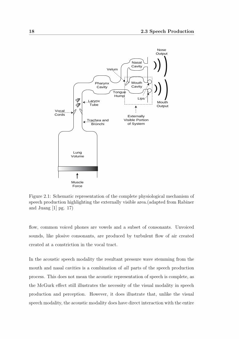
(mouth) and nasal cavity (nose). A simplified representation of the complete
physiological mechanism for creating speech is shown in Figure 2.1. The lungs
and associated muscles act as the source of air exciting the vocal mechanism. The
muscle force pushes air out of the lungs and through the bronchi and trachea.
Speech sounds can be classified into voiced and unvoiced sounds. Voiced sounds
are produced when the vocal cords are tensed incurring a vibration from the air
18 2.3 Speech Production
Lung Volume
Muscle Force
Vocal Cords
Larynx Tube
Trachea and Bronchi
Pharynx Cavity
Mouth Cavity
Nasal Cavity
Velum)) ))) )
Nose Output
Mouth Output
Externally Visible Portion
of System
Tongue Hump
Lips
Figure 2.1: Schematic representation of the complete physiological mechanism ofspeech production highlighting the externally visible area.(adapted from Rabinerand Juang [1] pg. 17)
flow, common voiced phones are vowels and a subset of consonants. Unvoiced
sounds, like plosive consonants, are produced by turbulent flow of air created
created at a constriction in the vocal tract.
In the acoustic speech modality the resultant pressure wave stemming from the
mouth and nasal cavities is a combination of all parts of the speech production
process. This does not mean the acoustic representation of speech is complete, as
the McGurk effect still illustrates the necessity of the visual modality in speech
production and perception. However, it does illustrate that, unlike the visual
speech modality, the acoustic modality does have direct interaction with the entire
2.4 Speech Reading 19
speech production mechanism. From Figure 2.1 it becomes clear in the visual
speech modality that, even in the best conditions, only the lips, teeth, frontal
tongue and jaw are externally visible. Important components like the vibration
of the vocal cords, soft palate (velum) and complete tongue shape cannot be
observed visually.
One theory for the advantage of combining the acoustic and visual speech modal-
ities can be found in [10], which notes that the part of the acoustic speech signal
that best describes the place of visible articulators lies in the higher frequency
component. This higher frequency component in the acoustic domain is more
susceptible to noise and hence more confusable. Whereas the non-visible articu-
lators are more closely related to the low frequency components of the acoustic
speech signal, which are more robust in the presence of noise.
2.4 Speech Reading
Speech reading, or as it is commonly referred to lip reading, refers to using visual
speech information such as lip movements to understand speech. Speech reading
is simply a special case of audio-visual speech recognition where all emphasis
is placed on the visual, not the acoustic, speech modality. A person skilled in
speech reading is able to infer the meaning of spoken sentences by looking at
the configuration and the motion of visible articulators of the speaker. Although
sometimes referred to as lip reading, speech information does not stem solely
from labial configurations as the tongue and teeth position also act as additional
sources of information. It is however, largely agreed [12] that most information
pertaining to visual speech does stem from the mouth region of interest (ROI),
but significant help in comprehension comes also from the entire facial expression.
Speech reading skills are acquired at a young age, with Dodd [13] reporting that
toddlers can speech read familiar words when they reach 19 months of age. The
20 2.5 Audio-visual Integration
visual speech modality plays an important role in learning to speak. Mills [14] was
able to show that blind children are slower in the acquisition of speech production
than seeing children, for those sounds which have visible articulation. Frowein et
al. [15] have studied the importance of frame rates in speech reading. It has been
shown that speech recognition performance drops markedly below 15 Hz.
In addition to speech reading, there are many other ways in which humans can use
their sight to assist in aural communication. Visible speech provides a supplemen-
tal information source that is useful when the listener has trouble comprehending
the acoustic speech. Furthermore, listeners may also have trouble comprehend-
ing the acoustic speech in situations where they lack familiarity with the speaker,
such as listening to a foreign language or an accented talker. It has been shown
by Sumby and Pollack [16] that when noisy environments are encountered, visual
information can lead to significant improvement in recognition by humans. The
complementing and supplemental nature of visual speech can be used in such
speech processing applications as automated speech recognition, enhancement
and coding under acoustically noisy conditions.
2.5 Audio-visual Integration
One question that remains to be answered in AVSP is how the human brain takes
advantage of the complementary nature of audio-visual speech and integrates the
two information sources. There is some contention over terminology in AVSP [17],
pertaining to the different levels of integration possible. It is widely agreed [6,
17, 18] however, that the acoustic and visual modalities can be combined either
at the feature or the decision level. These two differing integration paradigms
commonly go under the guise of early integration (EI) and late integration (LI),
but the interpretation of what EI and LI strictly are can vary markedly depending
on perspective and the task at hand.
2.5 Audio-visual Integration 21
For example, in continuous audio-visual speech applications Dupont and Luet-
tin [18] interpret LI as combining decisions at the sentence level. However, in
earlier literature [6, 19, 20], specifically for the tasks of isolated word recogni-
tion, LI is interpreted as combining decisions at the word unit level, irrespective
of whether continuous or isolated word unit tasks are being considered. This is
the interpretation adhered to in this thesis, as it seems a moot point to consider
combination at any level higher than this.
Similarly one hypothesis [6] for EI suggests that visual speech information is
converted to a vocal tract function, where then the acoustic and visual transfer
functions are averaged during integration. Alternatively EI can be interpreted [6,
18, 21] as the concatenation of acoustic and visual stimuli for processing as a
single observation.
In this thesis for the task of isolated word speech and speaker recognition three
broad levels of integration have been defined namely,
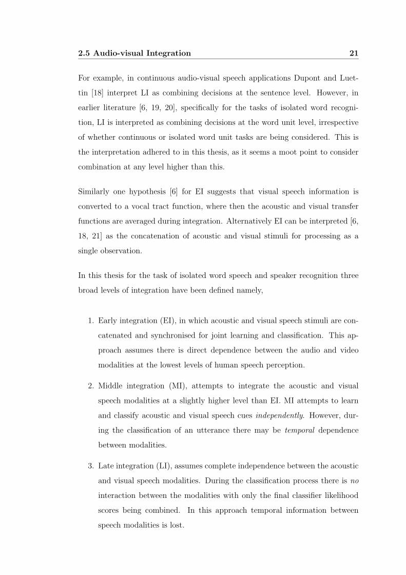
1. Early integration (EI), in which acoustic and visual speech stimuli are con-
catenated and synchronised for joint learning and classification. This ap-
proach assumes there is direct dependence between the audio and video
modalities at the lowest levels of human speech perception.
2. Middle integration (MI), attempts to integrate the acoustic and visual
speech modalities at a slightly higher level than EI. MI attempts to learn
and classify acoustic and visual speech cues independently. However, dur-
ing the classification of an utterance there may be temporal dependence
between modalities.
3. Late integration (LI), assumes complete independence between the acoustic
and visual speech modalities. During the classification process there is no
interaction between the modalities with only the final classifier likelihood
scores being combined. In this approach temporal information between
speech modalities is lost.
22 2.5 Audio-visual Integration
The distinction between EI, MI and LI is made in this thesis between how the
audio-visual classifier is trained and tested, not on directly whether the integration
has occurred at a feature or decision based level. This interpretation is of benefit
as it allows one to model audio-visual speech in terms of practical classifiers,
with the differences in synchronisation between the acoustic and visual modalities
as well as differences from integrating at a feature or decision level naturally
emerging as a consequence of these different training and testing approaches.
EI for audio-visual speech [6, 19] and speaker [21] recognition have been widely
used, and are of benefit as they model the dependencies between acoustic and
visual speech modalities directly. EI approaches suffer in two respects. Firstly,
if the acoustic or visual speech modalities are corrupted then the entire speech
modality is corrupted due to classification occurring at such a low level. Sec-
ondly, there is an assumption that the acoustic and visual speech modalities are
synchronised.
Lavagetto [12] demonstrated that acoustic and visual speech stimuli are not syn-
chronous, at least at a feature based level. It was shown that visible articulators,
during an utterance, start and complete their trajectories asynchronously, ex-
hibiting both forward and backward coarticulation with respect to the acoustic
speech wave. Intuitively this makes a lot of sense, as visual articulators (i.e. lips,
tongue, jaw) have to position themselves correctly before and after the start and
end of an acoustic utterance. This time delay is known as the voice-onset-time
(VOT) [18], which is defined as the time delay between the burst sound, coming
from the plosive part of a consonant, and the movement of the vocal folds for
the voiced part of a voiced consonant or subsequent vowel. McGrath et al. [22]
also found an audio lead of less than 80ms or lag of less than 140ms could not be
detected during speech. However, if the audio was delayed by more than 160ms
it no longer contributed useful information. It was concluded that, in practice,
delays of up to 40ms are acceptable. In normal PAL video this sample rate rep-
resents a single frame of asynchrony, signifying the importance of some degree of
2.5 Audio-visual Integration 23
asynchrony and synchrony in continuous audio visual speech perception.
LI is able to largely circumvent these problems. For automated isolated word ap-
plications LI strategies have reported superior results to EI for speech [6, 19, 20,
23, 24, 25] and speaker recognition [26, 27] tasks. LI allows for the asynchronous
classification of speech and can emphasise or deemphasise the importance of a
modality in classification depending on the corruption present. However, any
static or temporal dependencies occurring between modalities is lost. As pre-
viously mentioned LI has not proven as effective in continuous speech applica-
tions [18] where integration is attempted at greater than the word unit level.
Waiting until the end of the spoken utterance before combining modalities, as
the LI strategy was perceived by Dupont and Luettin [18], introduces an unde-
sirable time delay. To this end some form of synchrony is required.
The question remains at what level should audio-visual speech be synchronised.
MI allows for such synchrony whilst still providing a framework for guarding
against corruption in either modality. MI based approaches allow for the follow-
ing [18],
1. synchronous multimodal continuous speech recognition;
2. asynchrony of the visual and acoustic streams with the possibility to define
phonological resynchronisation points;
3. specific acoustic and visual word or sub-word models.
MI based approaches have been used to great success in continuous audio-visual
speech applications [18, 24, 28]. However the benefit of MI over LI, if LI is
constrained to be synchronised at the word unit level, is still not clear.
24 2.6 Visual Speaker Dependencies
2.6 Visual Speaker Dependencies
In recent research it has been shown that certain speaker dependent characteris-
tics exist in a speaker’s static mouth appearance as well as temporal pronuncia-
tion [4, 26, 29]. Speaker dependencies would be expected to be present in static
mouth parameters such as lip size, oral cavity size and lip colour [4]. Other tem-
poral parameters such as rate of lip movement or the amount of teeth and tongue
present, would be speaker dependent features which could be accumulated over
time. The speaker discrimination present in such a representation can readily be
used in a text-dependent speaker recognition system.
Speaker dependencies can also drastically affect automatic speech reading perfor-
mance. It has been reported by Potamianos et al. [30] that a speaker dependent
speech reading system, for a vocabulary of 26 words, attains an WER of 36.4%
in isolated word identification. Whereas the speaker independent speech reading
system, trained across 49 speakers, attains a very poor WER of 69.7%. This large
contrast in WER indicates speaker variabilities can inadvertently compromise the
performance of an automated speech reading system. Potamianos also reported
that steps that attempted to normalise for speaker variation generally improved
WER performance.
2.7 Speech Enhancement and Coding
The complementary nature of speech can be used for enhancement and coding as
well as recognition. Attempts have been made to estimate the clean spectral en-
velope of acoustic speech in noisy situations using visual features for the purposes
enhancement and coding. Researchers have tried to convert mouth movements
into acoustic speech directly [6]. In [31], a system called ‘image-input micro-
phone’ was built to take the mouth image as input, analyse the lip features such
as mouth width and height, and derive the corresponding vocal-tract transfer
2.7 Speech Enhancement and Coding 25
function.
In a series of papers [32, 33] a group of French researchers have proposed a frame-
work to map from the visual to the acoustic domain of speech. A new idea was
proposed, namely a system for enhancing noisy speech with the help of filters
using the speaker’s lip information. The idea was to use multivariate linear re-
gression to try and estimate the spectral envelope of a speech frame directly from
visible static labial information. Reflection coefficients were chosen to represent
the speech spectrum as they can be ensured to make the autoregressive filter
describing the speech frame spectrum stay stable. This technique was tested on
a small set of French oral vowels that are labially distinctive. The results were
obtained for an order 20 AR filter describing the speech spectrum and using the
inner labial width, height and area as the visual parameters. The results showed
there is a clear correlation between static lip shape and the synchronised spec-
tral envelope for that frame. This supports the findings in Section 2.2 on visual
phonetics that mentioned most visemes can be described by stationary images.
Unfortunately, there is a problem when the multivariate linear regression tech-
nique is ported over to processing continuous speech. This problem is most pro-
found in vowels. Vowels are basically classified into broad groups based on where
the tongue is positioned in the mouth (ie. front, mid and back). Without this
detailed information of where the tongue is in the mouth, the linear regression
technique turns into a non-linear problem with the same lip shape correspond-
ing to a number of different spectral envelopes. The same can be said for other
phoneme types such as plosives, dipthongs etc. This turns the problem into a
highly non-linear problem with different linear associators required for different
phoneme subsets. Girin, used a very basic spectral selector for his vowel exper-
iments so as to distinguish between the different vowel sets. This selector was
implemented thanks to linear discriminant analysis which was able to learn the
contrast between bark-scaled spectra of front vs back vowels. The system worked
quite well for extended vowel sets but a more complicated system was required
26 2.8 Chapter Summary
if the system was to be implemented for continuous speech. In a later paper [34]
they improved the associator by using multi-layered perceptrons so as to model
the non-linear relationship between acoustic and visual features more accurately.
It was shown that in the context of vowel-consonant-vowel transitions corrupted
with white noise, the performances of the system was improved in terms of the
intelligibility gain, distance measures and classification test.
The techniques used by Girin, Feng and Schwartz [32] for bimodal speech enhance-
ment were also used for bimodal speech coding by Foucher, Girin and Feng [33].
Using an associator to map from the visual to the acoustic domain a classical
vocoder was able to reduce the transmission rate from 2.4 kbit/s to 1.9 kbit/s by
estimating acoustic parameters from visual ones.
2.8 Chapter Summary
This chapter has given insights into modern AVSP from a theoretical and prag-
matic perspective. The complementary nature of the acoustic and visual speech
modalities has been discussed. The importance of acoustic and visual phonetics,
along with an understanding of the basic mechanics of speech production and
perception, has been established for the field of AVSP. Visible articulators other
than the lips (i.e. tongue, jaw and teeth) have been shown to be very important
in speech production and perception. Questions pertaining to what visual artic-
ulators and representations are effective for visual speech processing have been
raised. The speaker dependent nature of the visual speech modality has been
noted with their benefits
Strategies for integrating the acoustic and visual modalities have been investi-
gated, with three broad levels of integration being available (i.e. EI, MI and
LI). The choice of integration strategy is of particular importance to AVSP, as
an understanding of how humans perceive bimodal speech can greatly aid in the

2.8 Chapter Summary 27
construction of effective automated AVSP systems. Work in alternative AVSP
research avenues, such as audio-visual speech enhancement and coding, has been
touched upon.

Chapter 3
Classifier theory
3.1 Introduction
Classification, in a broader sense, can be considered as the problem of estimating
density functions in a high-dimensional space and dividing the space into regions
or classes [35]. As mentioned in Chapters 1 and 2, AVSP requires a number of
classifiers to recognise complex patterns in different domains. These classifiers
are required to take on tasks as varied as recognising a spoken utterance, the
identification and verification of a subject, to locating the mouth on a subject’s
face.
In this chapter generalised classifier theory is presented along with specifics on
classifier design and implementation. The problem specific aspect of classifier se-
lection and design is discussed with particular emphasis on selecting the classifier
best suited for those tasks pertinent to AVSP. Differences between parametric,
non-parametric and discriminant classifiers are discussed and the problem spe-
cific situations of where they work best reviewed. Parametric classifier design
is discussed in depth, as these classifiers are used throughout this thesis for the
tasks of speech recognition, speaker recognition and mouth tracking.
30 3.2 Classifier Theory Background
3.2 Classifier Theory Background
Theoretically, the Bayes classifier [35] is the best classifier for any given pattern
recognition problem, as this classifier minimises the probability of classification
error. The true a posteriori probability that observation o belongs to class ωi
can be formulated using Bayes rule,
Pr(ωi|o) =P (ωi)p(o|ωi)
∑Nn=1 P (ωnp(o|ωn)
(3.1)
where N is the total number of classes, P (ωi) is the a priori probability of being
in class ωi and p(o|ωi) is the true conditional density function for class ωi. In
practice, a classifier will never output the true a posteriori probability but an
estimate [5],
P r(ωi|o) = Pr(ωi|o) + ε(o) (3.2)
The error ε(o) is due to the mismatch between the true and actual decision
boundaries caused by having a finite training sample and the unknown parametric
form of p(o|ωi) from where o was drawn. Given a finite and noisy data set,
different classifiers typically provide different generalisations by realising different
decision boundaries in this space [36]. This makes the job of classifier selection
and design very much dependent on the nature of the problem (i.e. problem
domain) and the amount of training observations available, such that ε(o) is
minimised.

3.3 Non-parametric Classifiers 31
3.3 Non-parametric Classifiers
In most pattern recognition problems the form of the underlying class density
function p(o|ωi) is unknown. Non-parametric procedures are able, to somewhat,
circumvent these problems using arbitrary distributions without the assumption
that the form of the underlying density functions is known. Common imple-
mentations, involve the use of Parzen-windows [35, 37] or kn nearest neighbor
estimation. These techniques work on the basic premise that if one places a cell
of volume V around o and capture n samples, k of which turn out to be labeled ωi
then the density estimate can be approximated as,
p(o|ωi) ≈k/n
V(3.3)
As n goes to infinity then an infinite number of samples will fall inside an infinitely
small volume making our estimate of p(o|ωi) increasingly accurate. A natural
extension of this idea is the nearest-neighbor classifier.
A nearest neighbor classifier seeks to find of n labeled train observations o the
single closest observation to the test observation o∗, where D(a,b) is the distance
metric used to measure the similarity of observation vectors a and b. Common
distance metrics for comparing two observations are the simple Euclidean,
D(a,b) = (a − b)′(a − b) (3.4)
and the Mahanalobis distance,
D(a,b) = (a − b)′W−1(a − b) (3.5)
where W is a weighting matrix. As n approaches infinity the performance of the
32 3.4 Discriminant Classifiers
nearest neighbor classifier shall approach twice the Bayes error [35, 37]. How-
ever, when n is relatively small the choice of D(a,b) can drastically affect the
performance of the classifier [38].
Techniques like the the nearest-neighbor classifier have found uses in techniques
where training data is limited for the classes being discriminated between. Tasks
such as face recognition, where only one or two training observations are available
per-class, use nearest-neighbor classifiers with good results [38, 39]. For tasks
where there is sufficiently large amounts of training data per class, non-parametric
classifiers are less attractive, due to problems concerning training data storage
and computational tractability.
3.4 Discriminant Classifiers
The use of discriminant classifiers in many pattern recognition problems has
become quite wide spread. Traditionally the discriminant function gi(o), that
is the function defining decision boundaries for class ωi, is formed as a direct
consequence of knowing p(o|ωi). In practice however, due to the uncertainty
associated with the true form of p(o|ωi), it is sometimes more effective to assume
one knows the parametric form of the discriminant function gi(o) rather than
calculating the boundary indirectly using the estimate of p(o|ωi).
Artificial Neural Networks (ANNs) can be interpreted as a discriminant classi-
fier [37]. ANNs are usually expressed in network diagrams, where the number
of inputs is dictated by the dimensionality of the input observation vector, and
the number of outputs is dictated by the number of classes. The most common
ANN is the multilayer perceptron (MLP) [40]. MLPs are general purpose, flexi-
ble, nonlinear models that given sufficient complexity and training observations,
can approximate virtually any function to any desired degree of accuracy [37]. In
particular, in the limit of an infinite number of training observations, the outputs
3.4 Discriminant Classifiers 33
of a trained MLP will approximate the true a posteriori probability for a given
observation in a least-squares sense [37]. MLPs are of major use when one has
little knowledge about the form of the problem or nature of the training obser-
vations. ANNs have been successfully used for problems as diverse as automatic
face detection [41, 42], and speech recognition [8] with some success.
Support Vector Machines (SVMs) are also another type of discriminative clas-
sifier [37, 43, 44], limited to the two class case. SVMs perform discrimination
by choosing nonlinear functions (i.e. support vectors) that map the input to a
higher-dimensional space. With appropriate nonlinear mappings to sufficiently
high dimensions, the training set observations can always be separated by a hy-
perplane. An important benefit of the SVM approach is that the complexity of
the resulting classifier is characterised by the number of support vectors rather
than the dimensionality of the transformed space. As a result, SVMs tend to
be less prone to problems of over fitting than some other methods. Like ANNs,
SVMs have found use in well defined discrimination problems such as face [44]
and object detection.
A major disadvantage with discriminant classifiers is their inter-class dependence.
The formation of the decision boundaries for gi(o) of class ωi requires intimate
knowledge of all other classes in the problem domain. Discriminant classifiers
have found their niche in problems where all classes are static and well defined,
with minimal mismatch between the train and test observation sets, these types of
conditions are typically found in object detection and computer vision problems.
Discriminant classifiers tend to be suboptimal in large applications, where it is
difficult to process all classes simultaneously (eg. speech recognition), due to the
sheer complexity of the models. Computational problems also occur when the
number of classes or nature of the classes (eg. train/test mismatch) change, as
found in subject recognition tasks where the number of classes (i.e. subjects)
varies all the time, new discriminant functions gi(o) have to be estimated to
account for change in the number of classes. Similarly, when unmatched train
34 3.5 Parametric Classifiers
and test conditions are encountered the discriminant functions gi(o) have to be
re-estimated to account for the new class decision boundaries.
3.5 Parametric Classifiers
Parametric classifiers are the classifier of choice for much of the work presented in
this thesis. The remainder of this chapter shall concentrate on the construction
and implementation of such classifiers. Parametric classifiers have many bene-
fits over other classifiers for particular tasks. These tasks usually involve large
amounts of labeled training observations, where there is some basic understand-
ing of the approximate parametric nature of the density function from which the
observations were drawn. Further, since density estimates are being calculated
directly, statistical theory can be easily applied within the framework to expand
and refine existing models.
Given enough training data the estimation of a priori probabilities P (ωi) is quite
rudimentary [37]. However, estimating the conditional density estimates p(o|ωi) is
far more difficult. Firstly, the amount of training observations one has at their dis-
posal rarely does justice to describing the complexity of p(o|ωi). Secondly, these
training observations give no information on how one should express p(o|ωi) para-
metrically. If one knows the number of parameters in advance, one can then use
the training observations to estimate values for these parameters so as to satisfy
a certain criterion, thus reducing the complexity of the problem. The criterion
used for estimating these parameters may vary according to the amount of train-
ing observations and the classifier being employed. Typically maximum-likelihood
(ML) techniques are employed to estimate these parameters [8, 35, 37, 45].

3.5 Parametric Classifiers 35
3.5.1 Maximum likelihood estimation
In a parametric classifier one assumes p(o|ωi) has a known parametric form λi,
and one has a collection of training observations according to N observation
sets, S1, . . . ,SN, with the observations Si having been drawn indepen-
dently according to the conditional density function p(o|ωi). It must be noted
that the observations in Si give no information about λj where i 6= j. Due to
this independence one can dispense with class distinction to simplify notation.
To show the effectiveness of the parametric estimation of p(o) one can calculate
the likelihood of λ with respect to the training data,
p(S|λ) =
Ri∏
r=1
p(or|λ) (3.6)
where R is the number of training observations o drawn from observation set S ∼
p(o). The ML estimate of λ is the value λ that maximises l(λ). Where l(λ) can
be defined as the log-likelihood,
l(λ).=
R∑
r=1
log p(or|λ) (3.7)
For analytical reasons it is easier to deal with the log-likelihood l(λ) than the like-
lihood p(S|λ), however since the logarithm is a monotonically increasing function,
maximising the log-likelihood with respect to λ is equivalent to maximising the
likelihood. One can write the solution as the argument λ that maximises the
log-likelihood,
λ = arg maxλ
l(λ) (3.8)
This maximisation can be found through standard matrix algebra and differential

36 3.5 Parametric Classifiers
calculus such that,
∇λl(λ) = 0 (3.9)
where for λ containing K free parameters,
∇λ.=
ddλ1
...
ddλK
(3.10)
An explicit global solution to λ can be found only in the simplest of cases, however
a local optimum can often be found through the expectation maximisation (EM)
algorithm [46].
3.5.2 Expectation maximisation algorithm
The expectation maximisation (EM) algorithm [46] iteratively estimates the like-
lihood of the training observations. Using a full sample of training observa-
tions S = o1, . . . ,oT the search for the best model λ can be expressed in the
following algorithm,
1. Initialise: set λ0 to initial value, i = 0
2. Expectation (E) step: compute l(λi)
3. Maximisation (M) step: λi+1 = arg maxλ l(λi)
4. Iterate: i = i+ 1, repeat steps 2-3 until l(λi) − l(λi−1) ≤ Th or i ≤ N
where N is the maximum number of iterations allowed, Th is a preset conver-
gence threshold. The EM algorithm performs differently to other optimisation

3.6 Gaussian Mixture Models 37
techniques, such as the gradient descent algorithm [37], as it finds the global op-
timum λi for a fixed λi−1. This optimum would not necessarily be found via
gradient search. Although not assuring a global maximum, the EM algorithm
has been shown effective for estimating maximised λ Gaussian mixture models
(GMM) and hidden Markov models (HMM) in practical scenarios [8, 45].
3.6 Gaussian Mixture Models
Gaussian mixture models (GMMs) have been used extensively as a classifier in
general pattern recognition [35, 37, 45]. Gaussian distributions naturally occur in
many phenomena and complex systems. The proliferation of Gaussian distribu-
tions in nature and most complex systems can be explained through the Central
Limit Theorem [37, 47], which states that the aggregate effect of a large number
of small, independent random disturbances will lead to a Gaussian distribution.
In extremely complicated phenomena, such as speech signals, this effect may lead
to distributions aptly described as a mixture of Gaussian distributions or GMM.
One of the powerful attributes of the GMM is its ability to form smooth approxi-
mations to arbitrarily-shaped densities. A Gaussian mixture density is a weighted
sum of M component densities, given by,
p(o|λ) =M∑
i=1
cibi(o) (3.11)
where o is a D-dimensional random observation vector, bi(o) is the component
density function for mixture i and ci is the mixture weights satisfying the con-
straint∑M
i=1 ci = 1. Each component density function bi(o) is a D-variate Gaus-
sian function of the form
bi(o) =1
(2π)D/2|Σi|12
exp
−1
2(o − µi)
′Σ−1i (o − µi)
(3.12)
with mean vector µi and covariance matrix Σi.
38 3.6 Gaussian Mixture Models
As with any parametric classifier, given a set of training observations S drawn
from p(o), two problems need to be addressed. Firstly, what parametric form
should λ take on? Secondly, given a specific parametric form of λ how does
one calculate parameters that best approximates the true density p(o) given a
training set of observations S.
3.6.1 Classifier complexity versus training set size
In the creation of any parametric classifier there always exists the dichotomy of
classifier complexity versus the training set size. As the complexity (i.e. number
of free parameters in λ) of a parametric classifier increases the number of training
observations required to fully describe all possible variations in these parameters
increases exponentially. However, having too few parameters to parametrically
describe a distribution, may not give an adequate representation of the conditional
class density function p(o|ω) from whence S was drawn. These conflicting forces
can achieve some sort of equilibrium by selecting an appropriate GMM form
and topology depending on the size of S and the nature of the problem domain.
A GMM can take on several parametric forms depending on the choice of covari-
ance matrices [45]. These forms are classified as,
Nodal covariance: the model λi, for class i, can have one covariance matrix
per Gaussian component.
Grand covariance: the model λi, for class i, has only one covariance matrix
for all Gaussian components.
Global covariance: the model λi, for class i, has a single covariance matrix
shared by all class models.
Nodal covariance GMMs are most commonly used as they allow the training
set S to dictate the form of λ. However, in the absence of sufficient amounts
3.6 Gaussian Mixture Models 39
of training data, grand and global covariance GMMs can be employed to better
approximate p(o), by making problem domain specific assumptions about the
nature of the mixture covariance matrices. These individual covariance matrices
may be full or diagonal, again depending on the nature of the problem domain and
the size of the training set. In speech processing [45] diagonal nodal covariance
GMMs have been empirically shown to perform best in most speech applications.
Determining the topology (i.e. number of Gaussian components M) in a GMM
is an important but difficult problem. There is no theoretical way to estimate
the number of mixture components a priori. The choice of M again comes down
to a trade off between classifier complexity and training set size. Normally, M is
selected through heuristic and empirical evidence.
Singularities are a common symptom of poorly trained GMMs. A singularity
occurs when trying to find the inverse of a given covariance matrix. If the variance
elements of that matrix are quite small then the determinant of that matrix will
tend to zero, resulting in a singularity when one tries to evaluate the likelihood
function. To avoid spurious singularities, a variance limiting constraint can be
applied [45, 48] during the training of a given GMM. For an arbitrary element σ2i
of mixture component i’s covariance matrix Σi and a minimum variance value
σ2min the constraint,
σ2i =
σ2i if σ2
i > σ2min
σ2min if σ2
i ≤ σ2min
(3.13)
is applied to the variance estimates after each EM iteration to avoid singularities
in the final model. The value of σ2min must be found empirically for each specific
feature set and model size.
40 3.6 Gaussian Mixture Models
3.6.2 GMM parameter estimation
Using the normalised likelihood,
Li(r) =cibi(or)
∑Mk=1 ckbk(or)
(3.14)
the following re-estimation formulas are used on each EM iteration,
µi =
∑Rr=1 Li(r)or
∑Rr=1 Li(r)
(3.15)
Σi =
∑Rr=1 Li(r)(or − µi)(or − µi)
′
∑Rr=1 Li(r)
(3.16)
ci =1
R
R∑
r=1
Li(r) (3.17)
Equations 3.15 to 3.17 are iterated until convergence occurs, in practice this
usually occurs after 10-20 iterations.
3.6.3 GMM initialisation
The EM algorithm is guaranteed to find a local maximum likelihood model re-
gardless of the starting point, but depending on where the model λ is initialised
convergence can occur at different local maxima. There is no optimal way to
initialise an GMM, however Reynolds [45] defined three major techniques that
have been shown empirically to perform well,
Pre-labelled: the training observation set S can be pre-labeled via some arbi-
trary construct. For example, in [45] speech training data for the purposes
3.7 Hidden Markov Models 41
of text independent speaker recognition was initialised based on the M
phonetic clusters each observation fell into. This technique suffers from
the drawback that the M labels may not adequately represent the actual
number of mixtures present in the training set.
Random: this approach consists of choosing M observations from the training
set to use as the initial model means each with an identity matrix for
the starting covariance matrix. Although this approach is able to have
a variable number of M mixtures, its performance can vary dramatically
depending on which observations are chosen as the initial means.
K-means: a binary k-means clustering was used for initialisation [45, 49]. This
approach is able to cluster the training set into M clusters based on a
distance measure which is assured of reaching a local minimum based on
the chosen distance metric. To ensure stable clustering a binary splitting
approach is employed that iteratively generates M clusters. This approach
works by continually splitting the existing number of clusters in two, after
convergence, until there are M clusters. This approach is of use as one can
vary the number of initial mixtures M as well as being partially assured of
a stable initial estimate.
All experiments in this thesis, concerning GMMs, were conducted using initiali-
sation through binary k-means clustering.
3.7 Hidden Markov Models
Hidden Markov models (HMMs) are a well known mathematical tool for gaining a
stochastic model of temporal or spatial observations. HMMs can be easily applied
to spatial or temporal problems but, for purposes of explanation the temporal
case shall be used in this section. HMMs attempt to generate a model to describe
a set of observations, assuming they came from some unknown or hidden Markov

42 3.7 Hidden Markov Models
process whose internal states are not directly observable. A Markov process may
be described at any time as being in one of a set of N distinct states [8] as depicted
in Figure 3.1. At regularly spaced, discrete times, this process undergoes a change
of state according to a set of probabilities associated with the state.
2
1 3
PSfrag replacements
a11
a12
a13
a22
a21
a23
a33
a31
a32
Figure 3.1: Discrete states in a Markov model are represented by nodes and, thetransition probabilities by links.
Given the sequence of states q, defined as
q = q1, q2, . . . , qT, qt ∈ [1, 2, . . . , N ] (3.18)
where qt is the state at time t, one can obtain a probabilistic description that
our model λ generated the sequence q. Normally, a full probabilistic description
of the sequence q would, in general, require specification of the current state at
time t, as well as all the predecessor states. However, for the special case of a
discrete-time, first order, Markov chain, the probabilistic dependence is truncated
to just the preceding state,
Pr(qt = j|qt−1 = i, qt−2 = k, . . .) = Pr(qt = j|qt−1 = i) (3.19)
This notation can be further simplified if one realises the right side of Equa-
tion 3.19 is independent of time, leading to the set of state transition probabili-
ties A = aij of the form,

3.7 Hidden Markov Models 43
aij = Pr(qt = j|qt−1 = i) (3.20)
with the following properties,
ai,j ≥ 0 ∀j, i∑N
j=1 ai,j = 1 ∀i(3.21)
At time t = 1 one must have initial state probabilities πi,
πi = Pr(q1 = i), 1 ≤ i ≤ N (3.22)
So given a state sequence q and a Markov model λ = (A, π) one can gain an a
posteriori probability that q was created by λ,
Pr(q|λ) =∏T
t=1 Pr(qt|λ)
= πq1aq1q2aq2q3 . . . aqT−1qT
(3.23)
3.7.1 Hidden states
Unfortunately, in practice one does not have access to the state sequence q.
Instead, one can gain some observation feature vectors ot at time t from the
phenomena that is being modelled. The sequence O of observation vectors can
be expressed as,
O = o1,o2, . . . ,oT (3.24)
Therefore, the a posteriori probability that λ generated the observation O can
be given by,
Pr(O|λ) =∑
all q
Pr(O|q,λ)Pr(q|λ) (3.25)
Due to the class independent nature of an HMM it is simpler in practice to eval-
uate Equation 3.25 using conditional density functions for the case of continuous
HMMs, so without a loss of classification accuracy,
44 3.7 Hidden Markov Models
p(O|λ) =∑
all q
p(O|q,λ)Pr(q|λ) (3.26)
The term continuous HMM is used here to describe HMMs that model continuous
observations rather than quantizing the observations into discrete symbols known
as a discrete HMM [8]. Continuous HMMs have been found to be far more
effective than discrete HMMs in most applications such as speech processing [8].
To evaluate Equation 3.26 one needs to gain a value for p(O|q,λ) which can be
expressed, assuming statistical independence of observations as,
p(O|q,λ) =∏T
t=1 p(ot|qt,λ)
=∏T
t=1 bqt(ot)
(3.27)
where B = bj(ot) is compact notation expressing the likelihood of observa-
tion ot lying in state j. Throughout this chapter bj(ot) shall be evaluated in
parametric form as a mixture of Gaussians bjm(ot),
bj(ot) =∑Mj
m=1 cjmbjm(ot)
=∑Mj
m=1 cjmN (ot,µjm,Σjm)(3.28)
where, c is the mixture weight, µ is the mixture mean and Σ is the mixture
covariance matrix, for mixture m and state j. Gaussian mixture models (GMMs)
were discussed as a classifier in their own right in Section 3.6.
Using Equations 3.26 and 3.27 one should be able compute a likelihood of O being
generated by the hidden Markov model λ = (A,B, π). In reality however, the
computation of Equation 3.25 involves in the order of 2T ×N T calculations. This
calculation is computationally infeasible, so without much loss in performance
the Viterbi approximation [48, 50] is employed,
log p(O|λ) ≈ 1T
log p(O,q∗|λ)
≈ 1T(log πq∗(1)bq∗(1)(o1) +
∑Tt=2 log aq∗(t),q∗(t−1)bq∗(t)(ot))
(3.29)
3.7 Hidden Markov Models 45
where q∗ is the optimal state path that maximises Equation 3.29. This equation
is usually referred to as the Viterbi approximation, which is often used for recog-
nition without much loss in performance [48, 50]. Normalisation by 1T
is essential
so as to ensure the likelihood estimate received is not a function of the length
of the observation O. The optimal path q∗ is found in practice via the Viterbi
decoding algorithm [8, 48].
3.7.2 Viterbi decoding algorithm
The Viterbi decoding algorithm endeavors to find the most likely sequence of
hidden states q∗, for a given sequence of observations O, that was generated by
the model λ. To find q∗ one could consider enumerating every possible path
and calculating the likelihood, this is prohibitive in practice. There are several
ways to solve the problem of finding the optimal path q∗ associated with a given
observation sequence. The difficulty arises in the definition of the optimal state
sequence. The most common optimality criterion [8, 37] is to choose states qt that
are individually most likely at each time t. Although this criterion is optimal
locally there is no guarantee that the path is a valid one, as it might not be
consistent with the underlying model λ. However, it has been shown [8, 37] that
this locally optimal solution; works effectively in practice and can be formalised
into what is known as the Viterbi algorithm [1, 8, 37],
1. Initialisation:
δi(1) = πibi(ot), 1 ≤ i ≤ N
ψi(1) = 0(3.30)
2. Recursion:
δj(t) = bj(ot) maxNi=1 δi(t− 1)ai,j 2 ≤ t ≤ T, 1 ≤ j ≤ N
ψj(t) = arg maxNi=1 δi(t− 1)ai,j 2 ≤ t ≤ T, 1 ≤ j ≤ N
(3.31)
46 3.7 Hidden Markov Models
3. Termination:
p(O|q∗,λ) = maxNi=1 δi(T )
q∗T = arg maxNi=1 δi(T )
(3.32)
4. Path backtracking:
q∗t = ψq∗t+1(t+ 1), t = T − 1, T − 2, . . . , 1 (3.33)
where δi(t) is the best score along a single path, ψi(t) is an array to keep track of
the argument that has the maximum value, all for at time t. In practice a closely
related algorithm using logarithms [8] is employed, thus negating the need for
any multiplications reducing computation load considerably.
3.7.3 HMM parameter estimation
The goal of HMM learning is to determine model parameters λ = (A,B, π)
from a set of training observations Or, 1 ≤ r ≤ R, where R is the number of
training sequence observations. There is no known way to analytically solve for
the model parameter set that globally maximises the likelihood of the observation
in a closed form [8]. However, a good solution can nearly be always determined
by a straightforward technique known as the Baum-Welch or forward-backward
algorithm [37].
Whilst HMMs are considerably more complex than other parametric classifiers
dealt with in this chapter, it must be stressed that the same underlying ideas
are exploited. As with its simpler GMM cousin, one can choose λ that locally
maximises the likelihood p(O|λ) using an iterative procedure known as the Baum-
Welch algorithm which is an instance of the generalised expectation maximisation
(EM) algorithm [46]. Since this algorithm requires a starting guess for λ, some
form of initialisation must be performed [48]
3.7 Hidden Markov Models 47
Viterbi Training
Viterbi training for HMMs is analogous to k-means clustering for GMMs, in that
both techniques place a hard boundary on the observation sequence O. When
one initialises a new HMM, the Viterbi segmentation is replaced by a uniform
segmentation (i.e. each training observation is divided intoN sequal segments) for
the first iteration. After the first iteration, each training sequence Or is segmented
using a state alignment procedure which results from using the Viterbi decoding
algorithm described in Section 3.7.2 to get the optimal state sequence qr∗.
If Aij represents the total number of transitions from state i to state j in qr∗ for
all R observation sequences, then the transition probabilities can be estimated
from the relative frequencies,
aij =Aij
∑Nk=1Aik
(3.34)
Within each state, a further alignment of observations to mixtures components
is made by associating each observation ot with the mixture component with
the highest likelihood. On the first iteration unsupervised k-means clustering
is employed to gain an initial estimate for bj(ot), in a similar manner to the
initialisation procedures used for GMMs in Section 3.6.3. Viterbi training is
repeated until there is minimal change in the parameter model estimate λ.
Baum-Welch Re-Estimation
Baum-Welch training replaces the hard boundary segmentation used in Viterbi
training with a soft boundary denoted by L representing the likelihood of an
observation being associated with any given Gaussian mixture component. This
likelihood is known as the occupation likelihood [48] and is computed from the for-
ward and backward variables. The forward variable αi(t) is defined as,

48 3.7 Hidden Markov Models
αi(t) = p(o1o2 . . .ot, qt = i|λ) (3.35)
that is, the likelihood of the partial observation sequence o1o2 . . .ot and state i
at time t, given the model λ. Which can be solved inductively,
1. Initialisation:
αi(1) = πibi(o1), 1 ≤ i ≤ N (3.36)
2. Induction:
αj(t+ 1) =
[N∑
i=1
αi(t)aij
]
bj(ot+1), 1 ≤ i ≤ N, 1 ≤ t ≤ T − 1 (3.37)
In a similar manner, one can consider the backward variable βi(t) as,
βi(t) = p(ot+1ot+2 . . .oT |qt = i,λ) (3.38)
that is, the likelihood of the partial observation sequence ot+1ot+2 . . .oT and
state i at time t, given the model λ. Again, which can be solved inductively,
1. Initialisation:
βi(T ) = 1, 1 ≤ i ≤ N (3.39)
2. Induction:
βi(t) =N∑
j=1
aijbj(ot+1)βj(t+ 1), 1 ≤ i ≤ N, 1 ≤ t ≤ T − 1 (3.40)
If one inspects Equations 3.35 and 3.38 one notices αi(t) is a joint likelihood
where as βi(t) is a conditional likelihood such that,
p(O, qt = j|λ) = p(o1o2 . . .ot, qt = j|λ)p(ot+1ot+2 . . .oT |qt = j,λ)
= αj(t)βj(t)(3.41)

3.7 Hidden Markov Models 49
using Equation 3.41 one can define the likelihood of qt = j as Lj(t) in terms
of αj(t), βj(t) and λ,
Lrj(t) = p(qr
t = j|Or,λ)
=p(Or,qr
t =j|λ)
p(Or|λ)
= 1Prαr
j(t)βrj (t)
(3.42)
one can also define the likelihood of qrt = j for mixture component m as,
Lrjm(t) =
1
Pr
[N∑
i=1
αri (t− 1)aij
]
cjmbjm(ort )β
rj (t) (3.43)
where Pr is the total likelihood p(Or|λ) of the r’th observation sequence, which
can be calculated as,
Pr = αrN(T ) = βr
1(1) (3.44)
One can now re-estimate the transition probabilities A = aij using,
aij =
∑Rr=1
1Pr
∑Tr−1t=1 αr
i (t)aijbj(ort+1)β
rj (t+ 1)
∑Rr=1
1Pr
∑Tr−1t=1 αr
i (t)βri (t)
(3.45)
Given Equations 3.42, 3.43 and 3.44, one can now re-estimate mixture components
of B = bj(ot) = (cjm,µjm,Σjm),
µjm =
∑Rr=1
∑Tr
t Lrjm(t)or
t∑R
r=1
∑Tr
t Lrjm(t)
(3.46)
Σjm =
∑Rr=1
∑Tr
t Lrjm(t)(or
t − µjm)(ort − µjm)′
∑Rr=1
∑Tr
t Lrjm(t)
(3.47)

50 3.7 Hidden Markov Models
cjm =
∑Rr=1
∑Tr
t Lrjm(t)
∑Rr=1
∑Tr
t Lrj(t)
(3.48)
Equations 3.45 to 3.48 are iterated until convergence occurs, in practice this
usually occurs after 10 − 20 iterations.
Types of HMMs
HMMs are usually classified into different types by the structure of the transition
matrix A of the Markov chain. The general case of an ergodic HMM has been
considered where every state of the model could be reached, in a single step,
from every other state of the model. For speech processing [8, 37, 48] the left-
to-right type model has been found to account for the observed properties of
speech better than the standard ergodic model. The fundamental property of all
left-right HMMs is that the state-transition coefficients have the property,
aij = 0, j < i (3.49)
that is, no transitions are allowed to states whose indices are lower than that of
the current state. The initial state probabilities have the property,
πi
0, i 6= 1
1, i = 1(3.50)
The benefit of the left-to-right model in speech recognition can be found in the
constraints it imposes, which reduce the complexity of training while keeping
with the natural successive (i.e. left-to-right) nature of speech. Such a left-to-
right HMM is more restrictive than a general ergodic HMM in because it precludes
transitions back in time. Besides the two extremes of ergodic and left-to-right
HMMs, there are many other possible variations and combinations possible, which
are dealt with in Chapter 8 concerning multi-stream HMMs. It should be added,
3.8 Chapter Summary 51
that the imposition of constraints on an HMM model has no effect on the re-
estimation procedure, as any HMM parameter set to zero initially will remain at
zero throughout the re-estimation procedure.
3.8 Chapter Summary
In this chapter the topic of classifier theory was broached. The fundamental
theory behind classification theory was investigated, with the realisation that the
ideal Bayes classifier cannot be entertained in practice due to a finite amount
of training observations and the unknown parametric form of the conditional
class likelihood function p(o|ωi). From this realisation a number of classifier
types were investigated. Non-parametric classifier’s are of use in applications
where there is limited knowledge of the parametric form of p(o|ωi) and there is a
small amount of training observations, but start becoming cumbersome as more
and more training observations are entertained. Discriminant classifiers, such
as ANNs and SVMs, are excellent in circumstances when the number of classes
being distinguished between are static and train/test conditions are well matched.
They are of particular benefit when there is limited knowledge on the nature of
the problem. Parametric classifiers are the classifier of choice in this thesis. Unlike
discriminant classifiers, they have the ability to create a direct estimate p(o|ωi)
allowing for a varying number of classes, and due to their stochastic nature allow
for rigorous mathematical development.
The theory behind GMM based parametric classifiers was developed, and are
of benefit in problems where there is an assumption of independence between
observations. GMMs can be used in a plethora of classification tasks such as
object detection or pixel segmentation. HMM theory was developed for tasks
where there is some dependence between adjacent observations, such as in speech
signals. HMMs are used throughout this thesis for the tasks of speech recognition
and text dependent speaker recognition.

Chapter 4
Facial Feature Detection for
AVSP
4.1 Introduction
As discussed in Chapter 2, the visual speech modality plays an important role in
the perception and production of speech. Although not purely confined to the
mouth, it is generally agreed [12] that the large proportion of speech information
conveyed in the visual modality stems from the mouth region of interest (ROI).
To this end, it is imperative that an AVSP system be able to accurately detect,
track and normalise the mouth of a subject within a video sequence. This task is
referred to as facial feature detection (FFD) [51]. The goal of FFD is to detect the
presence and location of features, such as eyes, nose, nostrils, eyebrow, mouth,
lips, ears, etc., with the assumption that there is only one face in an image. This
differs slightly to the task of facial feature location which assumes the feature
is present and only requires its location. Facial feature tracking is an extension
to the task of location in that it incorporates temporal information in a video
sequence to follow the location of a facial feature as time progresses. Throughout
this chapter the tasks of facial feature detection, location and tracking are all
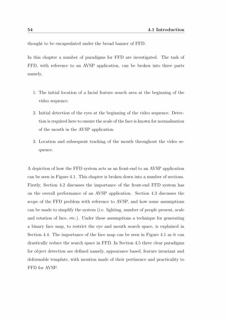
54 4.1 Introduction
thought to be encapsulated under the broad banner of FFD.
In this chapter a number of paradigms for FFD are investigated. The task of
FFD, with reference to an AVSP application, can be broken into three parts
namely,
1. The initial location of a facial feature search area at the beginning of the
video sequence.
2. Initial detection of the eyes at the beginning of the video sequence. Detec-
tion is required here to ensure the scale of the face is known for normalisation
of the mouth in the AVSP application.
3. Location and subsequent tracking of the mouth throughout the video se-
quence.
A depiction of how the FFD system acts as an front-end to an AVSP application
can be seen in Figure 4.1. This chapter is broken down into a number of sections.
Firstly, Section 4.2 discusses the importance of the front-end FFD system has
on the overall performance of an AVSP application. Section 4.3 discusses the
scope of the FFD problem with reference to AVSP, and how some assumptions
can be made to simplify the system (i.e. lighting, number of people present, scale
and rotation of face, etc.). Under these assumptions a technique for generating
a binary face map, to restrict the eye and mouth search space, is explained in
Section 4.4. The importance of the face map can be seen in Figure 4.1 as it can
drastically reduce the search space in FFD. In Section 4.5 three clear paradigms
for object detection are defined namely, appearance based, feature invariant and
deformable template, with mention made of their pertinence and practicality to
FFD for AVSP.
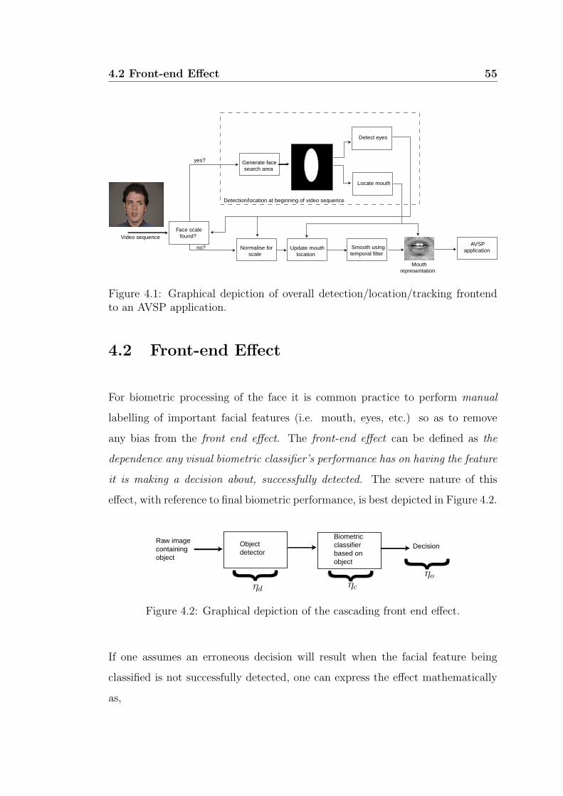
4.2 Front-end Effect 55
Generate face search area
AVSP application
Video sequence
Detect eyes
Locate mouth
Update mouth location
Detection/location at beginning of video sequence
Smooth using temporal filter
Face scale found?
yes?
Normalise for scale
no?
Mouth representation
Figure 4.1: Graphical depiction of overall detection/location/tracking frontendto an AVSP application.
4.2 Front-end Effect
For biometric processing of the face it is common practice to perform manual
labelling of important facial features (i.e. mouth, eyes, etc.) so as to remove
any bias from the front end effect. The front-end effect can be defined as the
dependence any visual biometric classifier’s performance has on having the feature
it is making a decision about, successfully detected. The severe nature of this
effect, with reference to final biometric performance, is best depicted in Figure 4.2.
Object detector
Biometric classifier based on object
Raw image containing object
Decision
PSfrag replacements
ηd ηc
ηo
Figure 4.2: Graphical depiction of the cascading front end effect.
If one assumes an erroneous decision will result when the facial feature being
classified is not successfully detected, one can express the effect mathematically
as,
56 4.3 Restricted Scope for AVSP
ηo = ηd × ηc (4.1)
where ηd is the probability that the object has been successfully detected, ηc is the
probability that a correct decision is made given the object has been successfully
detected and ηo is the overall probability that the system will make the correct
decision. Inspecting Equation 4.1 one can see that the performance of the overall
classification process ηo can be severely affected by the performance ηd of the
detector.
In ideal circumstances one wants ηd to approach unity, so one can concentrate on
improving the performance of ηc, thus improving the overall system performance.
A very simple way to ensure ηd approaches unity is through manual labelling
of facial features. Unfortunately, due to the amount of visual data needing to
be dealt with in an AVSP application, manual labelling is not a valid option.
The requirement for manually labelling facial features also brings the purpose
of any automatic classification system (i.e. speech or speaker recognition) into
question due to the need for human supervision. With these thoughts in mind,
an integral part of any AVSP application is the ability to make ηd approach unity
via an automatic FFD system and reliably keep it near unity to track that feature
through a given video sequence.
4.3 Restricted Scope for AVSP
As discussed in Section 4.2 accurate facial feature detection is crucial to any
AVSP system as it gives an upper bound on performance, due to the front-end
effect. FFD is a challenging task because of the inherent variability [51] from,
Pose: the images of a face vary due to the relative camera-face pose, with some
facial features such as an eye or nose becoming partially or wholly occluded.
4.3 Restricted Scope for AVSP 57
Presence or absence of structural components: facial features such as beards,
mustaches, and glasses may or may not be present adding a great deal of
variability in the appearance of a face.
Facial expression: a subject’s face can vary a great deal due to the subject’s
expression (e.g. happy, sad, disgusted, etc.).
Occlusion: faces may be partially occluded by other objects.
Image orientation: facial features directly vary for different rotations about
the camera’s optical axis.
Imaging conditions: when captured, the quality of the image, and facial fea-
tures which exist within the image, may vary due to lighting (spectra,
source distribution and intensity) and camera characteristics (sensor re-
sponse, lenses).
With over 150 reported approaches [51] to the field of face detection, the field is
now becoming well established. Unfortunately, from all this research there is still
no one technique that works best in all circumstances. Fortunately, the scope
of the facial feature detection task can be greatly narrowed due to the work in
this thesis being primarily geared towards AVSP. For any AVSP application, as
mentioned in Chapter 2, the main visual facial feature of importance is the mouth.
The extracted representation of the mouth does however, require some type of
normalisation for scale and rotation. It has been well documented [52] that the
eyes are an ideal measure of scale and rotation of a face. To this end, FFD
for AVSP will be restricted to eye detection and mouth detection, location and
tracking.
To further simplify the FFD problem for AVSP one can make a number of as-
sumptions about the images being processed,
• there is a single subject in each audio-visual sequence,
58 4.3 Restricted Scope for AVSP
• the subject’s facial profile is limited to frontal, with limited head rotation
(i.e. +/− 10 degrees),
• subjects are recorded under reasonable (both intensity and spectral) lighting
conditions,
• scale of subject remains relatively constant for a given video sequence.
These constraints are thought to be reasonable for most conceivable AVSP ap-
plications and are complied with in the M2VTS database [2] used throughout
this thesis for experimentation. Under these assumptions the task of FFD be-
comes considerably easier. However, even under these less trying conditions the
task of accurate eye and mouth detection and tracking, so as to provide suitable
normalisation and visual features for use in an AVSP application, is extremely
challenging.
4.3.1 Validation
To validate the performance of an FFD system, a measure of relative error [52]
is used based on the distances between the expected and the estimated eye posi-
tions. The distance between the eyes (deye) has long been regarded as an accurate
measure of scale of a face [52]. Additionally, the detection of the eyes is an in-
dication that the face search area does indeed contain a frontal face suitable for
processing with an AVSP system. The distances dl and dr, for the left and right
eyes respectively, are used to describe the maximum distances between the true
eye centers cl, cr ∈ R2 and the estimated positions cl, cr ∈ R2 as depicted in
Figure 4.3.
These distances are then normalised by dividing them by the distance between
the expected eye centers (deye = ‖cl − cr‖), making the measures independent of
the scale of the face in the image and the image size.
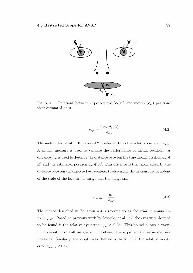
4.3 Restricted Scope for AVSP 59
PSfrag replacements cl cr
cm
dl dr
dm
cl cr
cm
Figure 4.3: Relations between expected eye (cl, cr) and mouth (cm) positionstheir estimated ones.
eeye =max(dl, dr)
deye
(4.2)
The metric described in Equation 4.2 is referred to as the relative eye error eeye.
A similar measure is used to validate the performance of mouth location. A
distance dm, is used to describe the distance between the true mouth position cm ∈
R2 and the estimated position cm ∈ R2. This distance is then normalised by the
distance between the expected eye centers, to also make the measure independent
of the scale of the face in the image and the image size:
emouth =dm
deye
(4.3)
The metric described in Equation 4.3 is referred to as the relative mouth er-
ror emouth. Based on previous work by Jesorsky et al. [52] the eyes were deemed
to be found if the relative eye error eeye < 0.25. This bound allows a maxi-
mum deviation of half an eye width between the expected and estimated eye
positions. Similarly, the mouth was deemed to be found if the relative mouth
error emouth < 0.25.
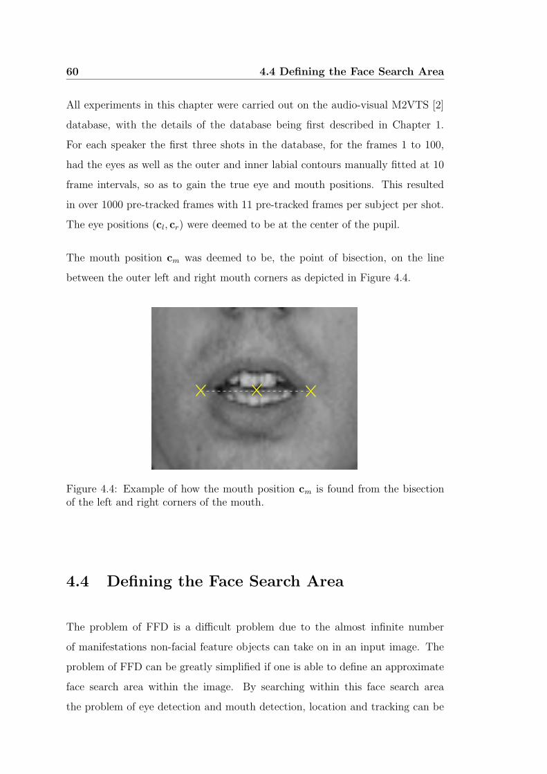
60 4.4 Defining the Face Search Area
All experiments in this chapter were carried out on the audio-visual M2VTS [2]
database, with the details of the database being first described in Chapter 1.
For each speaker the first three shots in the database, for the frames 1 to 100,
had the eyes as well as the outer and inner labial contours manually fitted at 10
frame intervals, so as to gain the true eye and mouth positions. This resulted
in over 1000 pre-tracked frames with 11 pre-tracked frames per subject per shot.
The eye positions (cl, cr) were deemed to be at the center of the pupil.
The mouth position cm was deemed to be, the point of bisection, on the line
between the outer left and right mouth corners as depicted in Figure 4.4.
Figure 4.4: Example of how the mouth position cm is found from the bisectionof the left and right corners of the mouth.
4.4 Defining the Face Search Area
The problem of FFD is a difficult problem due to the almost infinite number
of manifestations non-facial feature objects can take on in an input image. The
problem of FFD can be greatly simplified if one is able to define an approximate
face search area within the image. By searching within this face search area
the problem of eye detection and mouth detection, location and tracking can be
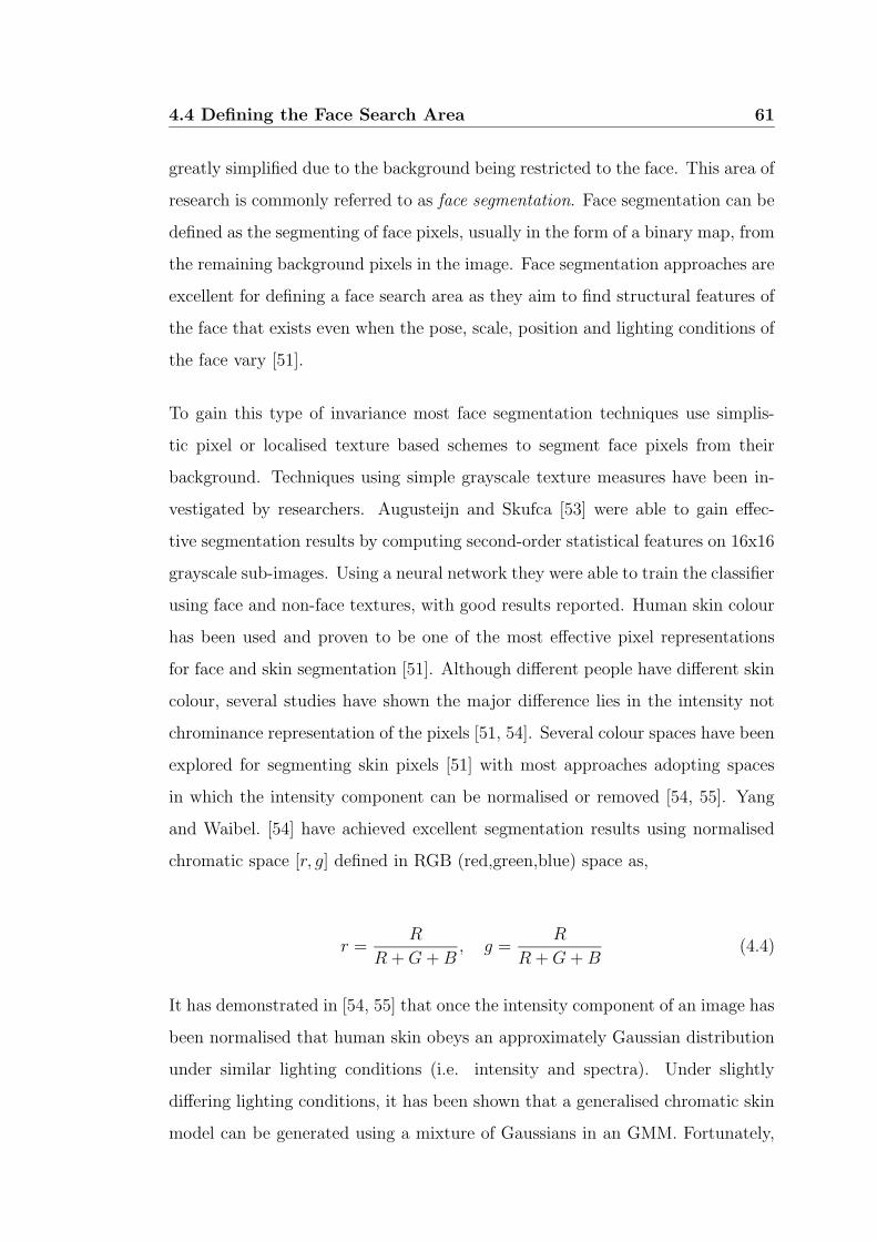
4.4 Defining the Face Search Area 61
greatly simplified due to the background being restricted to the face. This area of
research is commonly referred to as face segmentation. Face segmentation can be
defined as the segmenting of face pixels, usually in the form of a binary map, from
the remaining background pixels in the image. Face segmentation approaches are
excellent for defining a face search area as they aim to find structural features of
the face that exists even when the pose, scale, position and lighting conditions of
the face vary [51].
To gain this type of invariance most face segmentation techniques use simplis-
tic pixel or localised texture based schemes to segment face pixels from their
background. Techniques using simple grayscale texture measures have been in-
vestigated by researchers. Augusteijn and Skufca [53] were able to gain effec-
tive segmentation results by computing second-order statistical features on 16x16
grayscale sub-images. Using a neural network they were able to train the classifier
using face and non-face textures, with good results reported. Human skin colour
has been used and proven to be one of the most effective pixel representations
for face and skin segmentation [51]. Although different people have different skin
colour, several studies have shown the major difference lies in the intensity not
chrominance representation of the pixels [51, 54]. Several colour spaces have been
explored for segmenting skin pixels [51] with most approaches adopting spaces
in which the intensity component can be normalised or removed [54, 55]. Yang
and Waibel. [54] have achieved excellent segmentation results using normalised
chromatic space [r, g] defined in RGB (red,green,blue) space as,
r =R
R +G+B, g =
R
R +G+B(4.4)
It has demonstrated in [54, 55] that once the intensity component of an image has
been normalised that human skin obeys an approximately Gaussian distribution
under similar lighting conditions (i.e. intensity and spectra). Under slightly
differing lighting conditions, it has been shown that a generalised chromatic skin
model can be generated using a mixture of Gaussians in an GMM. Fortunately,
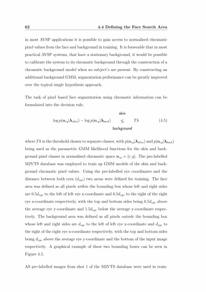
62 4.4 Defining the Face Search Area
in most AVSP applications it is possible to gain access to normalised chromatic
pixel values from the face and background in training. It is forseeable that in most
practical AVSP systems, that have a stationary background, it would be possible
to calibrate the system to its chromatic background through the construction of a
chromatic background model when no subject’s are present. By constructing an
additional background GMM, segmentation performance can be greatly improved
over the typical single hypothesis approach.
The task of pixel based face segmentation using chromatic information can be
formulated into the decision rule,
log p(org|λskin) − log p(org|λback)
skin
≶
background
Th (4.5)
where Th is the threshold chosen to separate classes, with p(org|λskin) and p(org|λback)
being used as the parametric GMM likelihood functions for the skin and back-
ground pixel classes in normalised chromatic space org = [r, g]. The pre-labelled
M2VTS database was employed to train up GMM models of the skin and back-
ground chromatic pixel values. Using the pre-labelled eye coordinates and the
distance between both eyes (deye) two areas were defined for training. The face
area was defined as all pixels within the bounding box whose left and right sides
are 0.5deye to the left of left eye x-coordinate and 0.5deye to the right of the right
eye x-coordinate respectively, with the top and bottom sides being 0.5deye above
the average eye y-coordinate and 1.5deye below the average y-coordinate respec-
tively. The background area was defined as all pixels outside the bounding box
whose left and right sides are deye to the left of left eye x-coordinate and deye to
the right of the right eye x-coordinate respectively, with the top and bottom sides
being deye above the average eye y-coordinate and the bottom of the input image
respectively. A graphical example of these two bounding boxes can be seen in
Figure 4.5.
All pre-labelled images from shot 1 of the M2VTS database were used in train-
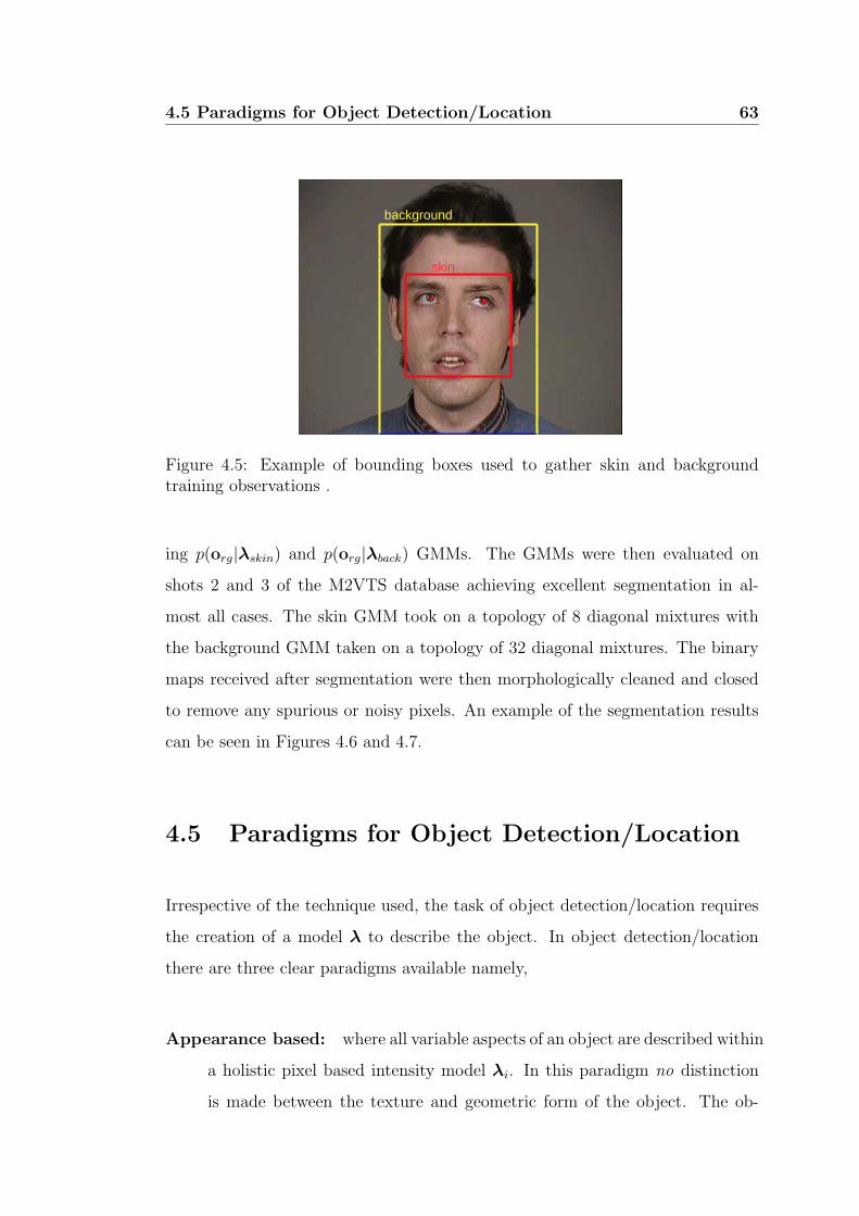
4.5 Paradigms for Object Detection/Location 63
background
skin
Figure 4.5: Example of bounding boxes used to gather skin and backgroundtraining observations .
ing p(org|λskin) and p(org|λback) GMMs. The GMMs were then evaluated on
shots 2 and 3 of the M2VTS database achieving excellent segmentation in al-
most all cases. The skin GMM took on a topology of 8 diagonal mixtures with
the background GMM taken on a topology of 32 diagonal mixtures. The binary
maps received after segmentation were then morphologically cleaned and closed
to remove any spurious or noisy pixels. An example of the segmentation results
can be seen in Figures 4.6 and 4.7.
4.5 Paradigms for Object Detection/Location
Irrespective of the technique used, the task of object detection/location requires
the creation of a model λ to describe the object. In object detection/location
there are three clear paradigms available namely,
Appearance based: where all variable aspects of an object are described within
a holistic pixel based intensity model λi. In this paradigm no distinction
is made between the texture and geometric form of the object. The ob-
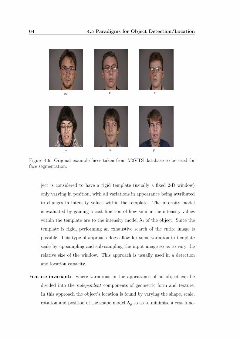
64 4.5 Paradigms for Object Detection/Location
pp lh fo
nv lc jd
Figure 4.6: Original example faces taken from M2VTS database to be used forface segmentation.
ject is considered to have a rigid template (usually a fixed 2-D window)
only varying in position, with all variations in appearance being attributed
to changes in intensity values within the template. The intensity model
is evaluated by gaining a cost function of how similar the intensity values
within the template are to the intensity model λi of the object. Since the
template is rigid, performing an exhaustive search of the entire image is
possible. This type of approach does allow for some variation in template
scale by up-sampling and sub-sampling the input image so as to vary the
relative size of the window. This approach is usually used in a detection
and location capacity.
Feature invariant: where variations in the appearance of an object can be
divided into the independent components of geometric form and texture.
In this approach the object’s location is found by varying the shape, scale,
rotation and position of the shape model λg so as to minimise a cost func-
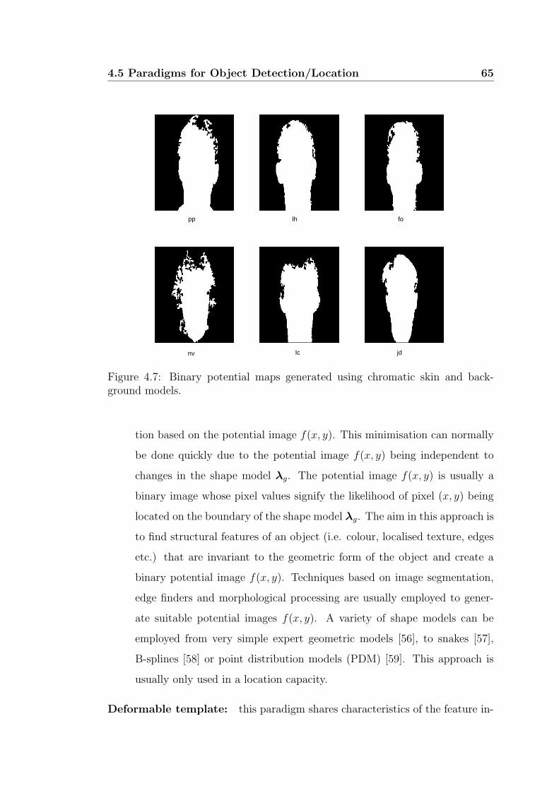
4.5 Paradigms for Object Detection/Location 65
pp lh fo
nv lc jd
Figure 4.7: Binary potential maps generated using chromatic skin and back-ground models.
tion based on the potential image f(x, y). This minimisation can normally
be done quickly due to the potential image f(x, y) being independent to
changes in the shape model λg. The potential image f(x, y) is usually a
binary image whose pixel values signify the likelihood of pixel (x, y) being
located on the boundary of the shape model λg. The aim in this approach is
to find structural features of an object (i.e. colour, localised texture, edges
etc.) that are invariant to the geometric form of the object and create a
binary potential image f(x, y). Techniques based on image segmentation,
edge finders and morphological processing are usually employed to gener-
ate suitable potential images f(x, y). A variety of shape models can be
employed from very simple expert geometric models [56], to snakes [57],
B-splines [58] or point distribution models (PDM) [59]. This approach is
usually only used in a location capacity.
Deformable template: this paradigm shares characteristics of the feature in-
66 4.5 Paradigms for Object Detection/Location
variant and rigid template paradigms. In a similar fashion to the rigid
template approach, the geometric form and intensity information of the ob-
ject are dependent on each other. In this approach however, the template
used to evaluate the intensity information of an object is non-rigid (i.e. can
move freely according to the shape model λg). The intensity model is eval-
uated by gaining a cost function of how similar the intensity values around
or within the template are to the intensity model describing the object. Un-
like the rigid template approach, an exhaustive search of the image using a
deformable template is computationally intractable due to the exponential
increase in the search space caused by the template being allowed to vary in
both shape and position. Such an operation can be made computationally
tractable by employing quicker minimisation techniques such as steepest de-
scent [47, 56], downhill simplex [24, 47] and genetic algorithms [60], allowing
such a detection/location approach to be computationally feasible.
The choice of paradigm to use is dependent on the type of object being detected
and the conditions under which it was captured. Appearance based approaches
have been used widely for FFD in the past with excellent results [39, 41, 42, 44,
51, 61] and are well suited to both the eye detection and mouth location/tracking
tasks due to their probabilistic nature. Feature invariant approaches have been
widely used for lip contour localisation and tracking. In lip contour localisation,
approaches using colour [58, 62, 63, 64], edges [65], as well as localised texture [63]
have been used to gain potential maps for a geometric model λg of the lips to be
fitted to, and the subsequent mouth center found. Similar techniques have been
devised for eye localisation, using intensity edge maps [56] and colour represen-
tations [52], but are of limited use for the eye detection task required in AVSP.
Both the appearance based and feature invariant paradigms, in Chapters 5 and 6
respectively, will be discussed and evaluated in-depth for the tasks of mouth
localisation and tracking.
4.5 Paradigms for Object Detection/Location 67
Deformable template approaches were first used by Yuille et al. [56] for mouth
and eye localisation using expert based appearance and shape models. In this ap-
proach an expert deformable template of the eyes and labial contour is fitted to an
intensity model, by calculating a cost function based on the grayscale intensity
edges, valleys and peaks around the templates boundary. The search strategy
uses the steepest descent algorithm to fit the template. Unfortunately, due to
the heuristic nature of the shape models λg and intensity models the approach
has poor performance when applied across a large number of subjects. Cootes et
al. [59] devised a similar technique for building a deformable template incorporat-
ing texture and shape models through exemplar learning. The technique used a
deformable template known as an active shape model (ASM). The ASM was able
to statistically learn allowable variations in shape of an object from pre-labelled
object shapes in a point distribution model (PDM) [59, 60]. Intensity informa-
tion about the object was also statistically learnt. In this approach a number
of grayscale profile vectors were extracted normal to set points around the de-
formable template. All these vectors were concatenated into a matrix known as
global profile vectors from which variations in intensity were statistically mod-
elled as a grey level profile distribution model (GLDM) [20, 60]. Luettin [24]
applied ASMs to lip contour localisation, using the downhill simplex minimisa-
tion technique to fit the lip shape model λg described by a PDM to an image
containing a mouth.
Matthews et al. [20] used another type of statistically learnt deformable template
approach to fit a lip shape model λg to an image containing a mouth. This type of
deformable template is referred to as an active appearance model (AAM) and was
first developed in [60]. This approach, similar in many respects to ASMs, uses a
PDM to statistically learn the shape variations of the object. The intensity model
for the object is learnt by warping the intensity information contained within the
deformable template back to the mean shape position. This warped intensity
information is then used to statistically model the distribution of intensity values
of an object whose shape has been normalised. The statistical nature of the in-
68 4.6 Chapter Summary
tensity model allows AAMs to be used for detection as well as location purposes.
AAMs have been applied to the task of lip contour detection/location, using a ge-
netic algorithm for minimisation [20]. ASMs and AAMs have been use with much
success in whole facial feature location, where an entire model of the face (i.e.
including the eyes, lips, nose and jawline) are detected/located. Unfortunately,
the minimisation techniques required to fit ASMs and AAMs are highly sensitive
to initialisation and do not guarantee convergence to an acceptable minimum.
Although deformable template approaches, namely ASMs and AAMs, have been
shown to be useful for face/eye detection and mouth location/tracking for AVSP
applications in literature [20, 24, 66], the problems associated with searching for
an minimum make detection/location performance largely unreliable and will not
be explored in this thesis for FFD pertaining to AVSP.
4.6 Chapter Summary
Facial feature detection (FFD) is a necessary front-end to any AVSP system.
In this chapter the two basis tasks of eye detection and mouth location/tracking
have been defined as being essential in any workable AVSP system. This task can
be in many respects simplified by restricting the scope of the problem (i.e. single
subject, frontal pose, static background, etc.), but still remains a very difficult
problem. Error metrics for evaluating the effectiveness of an FFD system have
also been defined. The use of skin maps, obtained via chromatic skin segmenta-
tion, have also been entertained as an additional way of reducing the FFD search
space.
Three paradigms for object detection/location have been defined namely, appear-
ance based, feature invariant and deformable template. The appearance based
and feature invariant based paradigms have proven effective for FFD and will be
pursued further in Chapters 5 and 6. The deformable template paradigm, due to
its complexity and instability, is deemed to be of little use in FFD for AVSP.
Chapter 5
Appearance Based Detection
5.1 Introduction
Appearance base detection techniques vary quite dramatically between approaches
[51], but all work on a similar premise. Appearance based approaches differ to
other detection techniques as knowledge about the shape and texture of the ob-
ject is learnt in a exemplar and holistic manner. That is to say, all knowledge
about an object is gained from a set of example intensity images without any a
priori knowledge about the object. This differs to other approaches where some
knowledge from an expert, about the object, is brought to bare on the problem
(i.e. a priori knowledge about the shape or texture of the object).
Appearance based detection schemes work by sliding a 2-D windowW (x, y) across
an input image, with the contents of that window being classified as belonging
to the object ωobj or background ωbck classes. The sliding of an n1 × n2 2-D
window W (x, y) across an N1 × N2 input image I(x, y) can be represented as
a concatenated matrix of vectors Y = [y1, . . . ,yT ]. Where the D = n1n2 di-
mensional random vector yt contains the vectorised contents of W (x, y) centered
at pixel coordinates (x, y). A depiction of this representation can be seen in
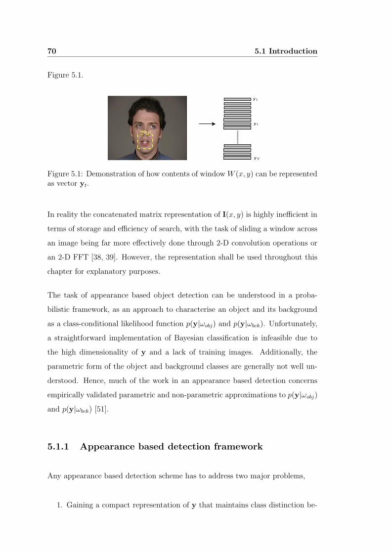
70 5.1 Introduction
Figure 5.1.
+ ..............W(x,y)
PSfrag replacements
y1
yt
yT
Figure 5.1: Demonstration of how contents of window W (x, y) can be representedas vector yt.
In reality the concatenated matrix representation of I(x, y) is highly inefficient in
terms of storage and efficiency of search, with the task of sliding a window across
an image being far more effectively done through 2-D convolution operations or
an 2-D FFT [38, 39]. However, the representation shall be used throughout this
chapter for explanatory purposes.
The task of appearance based object detection can be understood in a proba-
bilistic framework, as an approach to characterise an object and its background
as a class-conditional likelihood function p(y|ωobj) and p(y|ωbck). Unfortunately,
a straightforward implementation of Bayesian classification is infeasible due to
the high dimensionality of y and a lack of training images. Additionally, the
parametric form of the object and background classes are generally not well un-
derstood. Hence, much of the work in an appearance based detection concerns
empirically validated parametric and non-parametric approximations to p(y|ωobj)
and p(y|ωbck) [51].
5.1.1 Appearance based detection framework
Any appearance based detection scheme has to address two major problems,
1. Gaining a compact representation of y that maintains class distinction be-
5.1 Introduction 71
tween object and background sub-images, but is of small enough dimen-
sionality to create a well trained and computationally viable classifier.
2. Selection of a classifier to realise accurate and generalised decision bound-
aries between the object and background classes.
Most appearance based object detection schemes borrow heavily on principal
component analysis (PCA), or some variant, to generate a compact representation
of the sub-image y. PCA is an extremely useful technique for mapping an D
dimensional sub-image y into an M dimensional subspace optimally, in terms of
reconstruction error. A fundamental problem with PCA is that it seeks a subspace
that best represents a sub-image in a sum-squared error sense. Unfortunately,
in detection the criteria for defining an M dimensional subspace should be class
separation between the object and background classes not reconstruction error.
Techniques such as linear discriminant analysis (LDA) produce a sub-space based
on such a criterion for detection [35, 37, 51, 61]. However, most of these techniques
still require PCA to be used initially to provide a subspace that is free of any low
energy noise, that may hinder the performance of techniques like LDA [61, 67].
For this reason most successful appearance based detection schemes [39, 51] still
use PCA or variant to some extent [68, 69, 70] to represent the sub-image y
succinctly.
The choice of what classifier to use in facial feature detection is predominantly
problem specific. The use of discriminant classifiers such as artificial neural net-
works (ANNs) [51] and support vector machines (SVMs) [44, 51] has become pro-
lific in recent times. As discussed in Chapter 3, ANNs and SVMs are very useful
for classification tasks where the number of classes are static as they try to find
the decision boundary directly for distinguishing between classes. This approach
often has superior performance over parametric classifiers, such as Gaussian mix-
ture models (GMMs), as parametric classifiers form their decision boundaries
indirectly from their conditional class likelihood estimates. However, parametric
classifiers, such as GMMs, lend themselves to more rigorous mathematical devel-
72 5.1 Introduction
opment and allow for the compact representation and classifier problems, associ-
ated with appearance based detection, to be handled within the one framework.
In this chapter GMMs are used to gain parametric likelihood functions p(y|λobj)
and p(y|λbck) for facial feature detection experiments.
5.1.2 Principal component analysis
Principal component analysis (PCA) is a widely used dimensionality reduction
technique [35, 68]. It is optimal, in terms of mean squared error, as a linear scheme
for compressing a set of high dimensional vectors into a set of lower dimensional
vectors and then reconstructing them. This energy preserving characteristic of
PCA, or Karhunen-Loeve transform (KLT) as it sometimes referred to as [37],
makes it ideal as a feature extraction technique for high dimensional observations,
as the majority of energy in the observation can be represented in a lower and
easier to handle dimensionality. PCA is data driven, that is to say that all model
parameters can be computed directly from the data.
Given an ensemble Y = [y1, . . . ,yT ] of T observations yt of dimensionalityD with
zero mean µY = 0, one can express Y compactly, without loss of information as,
X(R×T ) = Φ(R×D)Y(D×T ) (5.1)
where Φ = [φ1, . . . ,φR] are the R eigenvectors (where R is the rank of ΣY =
1T−1
Y′Y) that diagonalises ΣY such that,
Λ = Φ′ΣYΦ (5.2)
given diag(Λ) = [λ1, . . . , λR], which for reasons that will become clear later are
ordered in descending order, where λi is the corresponding eigenvalue to the
eigenvector φi. In practical problems the rank of R can still be too large for use
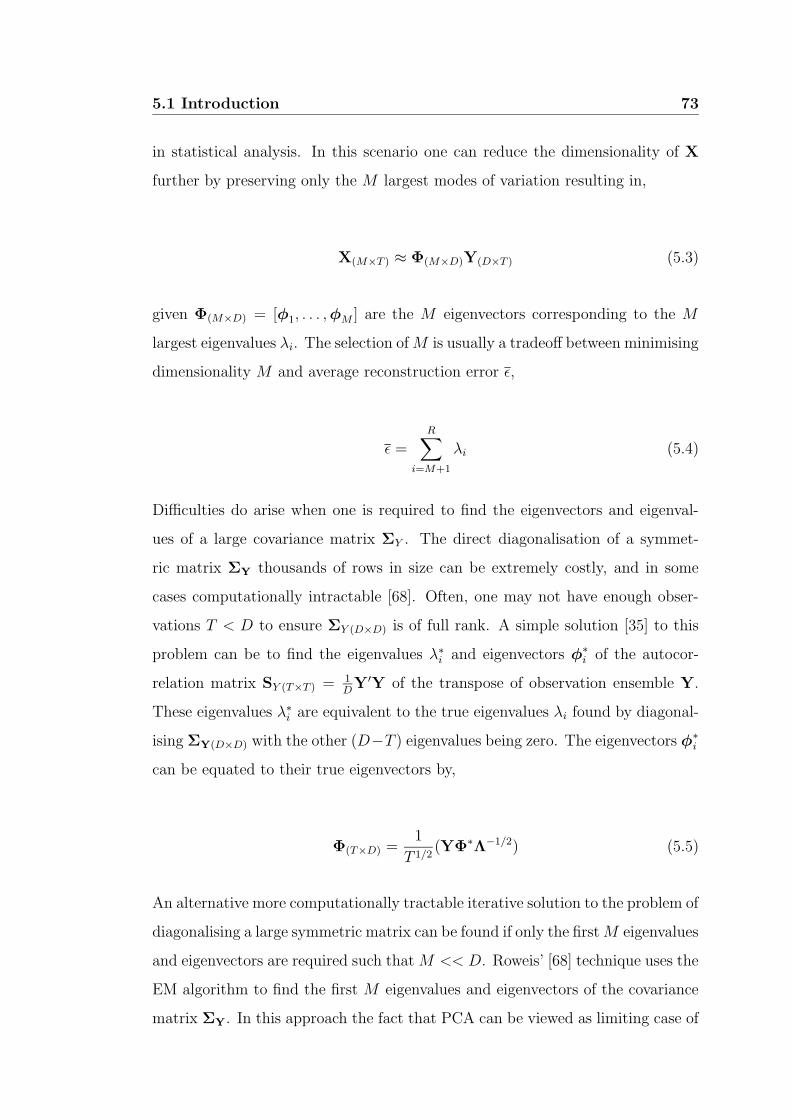
5.1 Introduction 73
in statistical analysis. In this scenario one can reduce the dimensionality of X
further by preserving only the M largest modes of variation resulting in,
X(M×T ) ≈ Φ(M×D)Y(D×T ) (5.3)
given Φ(M×D) = [φ1, . . . ,φM ] are the M eigenvectors corresponding to the M
largest eigenvalues λi. The selection ofM is usually a tradeoff between minimising
dimensionality M and average reconstruction error ε,
ε =R∑
i=M+1
λi (5.4)
Difficulties do arise when one is required to find the eigenvectors and eigenval-
ues of a large covariance matrix ΣY . The direct diagonalisation of a symmet-
ric matrix ΣY thousands of rows in size can be extremely costly, and in some
cases computationally intractable [68]. Often, one may not have enough obser-
vations T < D to ensure ΣY (D×D) is of full rank. A simple solution [35] to this
problem can be to find the eigenvalues λ∗i and eigenvectors φ∗
i of the autocor-
relation matrix SY (T×T ) = 1DY′Y of the transpose of observation ensemble Y.
These eigenvalues λ∗i are equivalent to the true eigenvalues λi found by diagonal-
ising ΣY(D×D) with the other (D−T ) eigenvalues being zero. The eigenvectors φ∗i
can be equated to their true eigenvectors by,
Φ(T×D) =1
T 1/2(YΦ∗Λ−1/2) (5.5)
An alternative more computationally tractable iterative solution to the problem of
diagonalising a large symmetric matrix can be found if only the firstM eigenvalues
and eigenvectors are required such that M << D. Roweis’ [68] technique uses the
EM algorithm to find the first M eigenvalues and eigenvectors of the covariance
matrix ΣY. In this approach the fact that PCA can be viewed as limiting case of
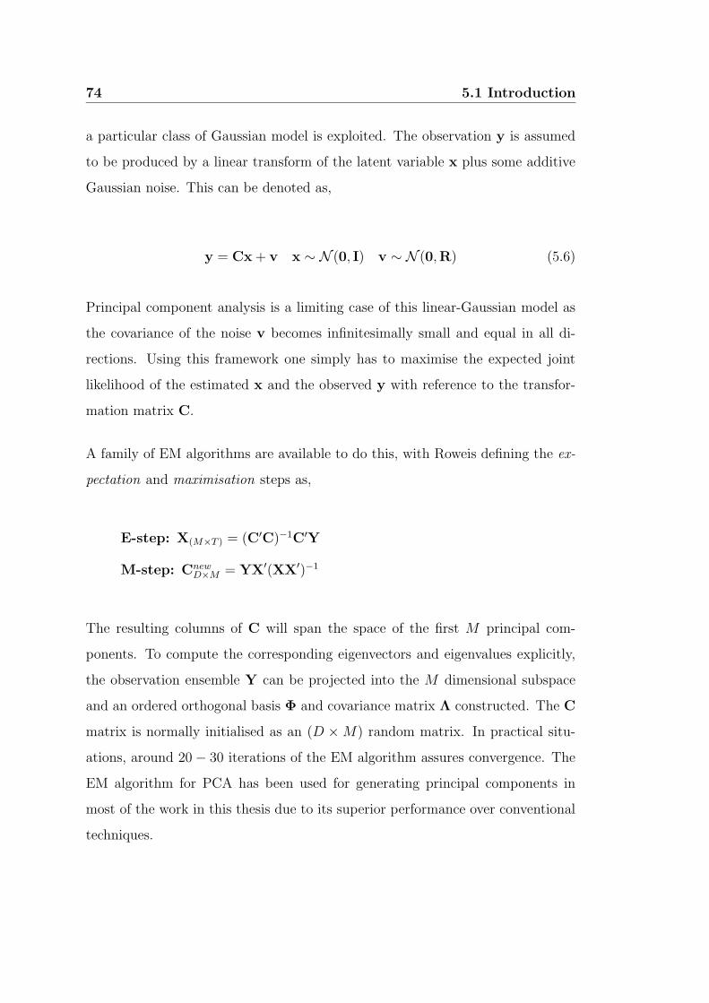
74 5.1 Introduction
a particular class of Gaussian model is exploited. The observation y is assumed
to be produced by a linear transform of the latent variable x plus some additive
Gaussian noise. This can be denoted as,
y = Cx + v x ∼ N (0, I) v ∼ N (0,R) (5.6)
Principal component analysis is a limiting case of this linear-Gaussian model as
the covariance of the noise v becomes infinitesimally small and equal in all di-
rections. Using this framework one simply has to maximise the expected joint
likelihood of the estimated x and the observed y with reference to the transfor-
mation matrix C.
A family of EM algorithms are available to do this, with Roweis defining the ex-
pectation and maximisation steps as,
E-step: X(M×T ) = (C′C)−1C′Y
M-step: CnewD×M = YX′(XX′)−1
The resulting columns of C will span the space of the first M principal com-
ponents. To compute the corresponding eigenvectors and eigenvalues explicitly,
the observation ensemble Y can be projected into the M dimensional subspace
and an ordered orthogonal basis Φ and covariance matrix Λ constructed. The C
matrix is normally initialised as an (D ×M) random matrix. In practical situ-
ations, around 20 − 30 iterations of the EM algorithm assures convergence. The
EM algorithm for PCA has been used for generating principal components in
most of the work in this thesis due to its superior performance over conventional
techniques.
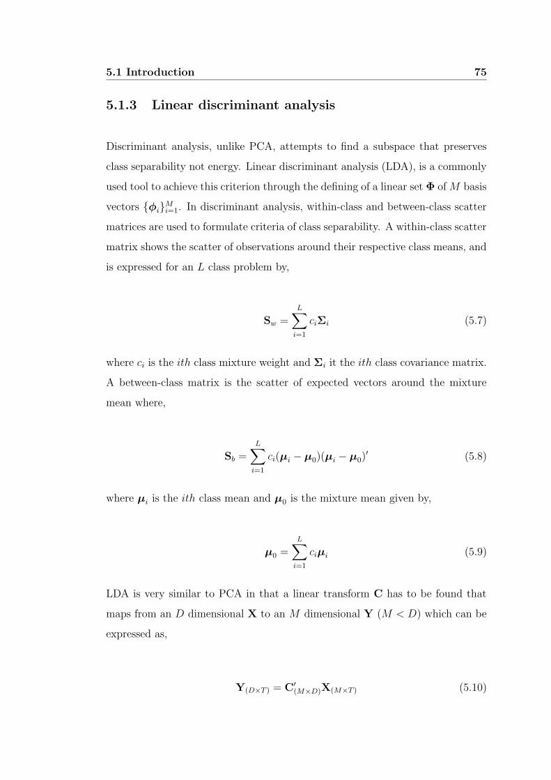
5.1 Introduction 75
5.1.3 Linear discriminant analysis
Discriminant analysis, unlike PCA, attempts to find a subspace that preserves
class separability not energy. Linear discriminant analysis (LDA), is a commonly
used tool to achieve this criterion through the defining of a linear set Φ of M basis
vectors φiMi=1. In discriminant analysis, within-class and between-class scatter
matrices are used to formulate criteria of class separability. A within-class scatter
matrix shows the scatter of observations around their respective class means, and
is expressed for an L class problem by,
Sw =L∑
i=1
ciΣi (5.7)
where ci is the ith class mixture weight and Σi it the ith class covariance matrix.
A between-class matrix is the scatter of expected vectors around the mixture
mean where,
Sb =L∑
i=1
ci(µi − µ0)(µi − µ0)′ (5.8)
where µi is the ith class mean and µ0 is the mixture mean given by,
µ0 =L∑
i=1
ciµi (5.9)
LDA is very similar to PCA in that a linear transform C has to be found that
maps from an D dimensional X to an M dimensional Y (M < D) which can be
expressed as,
Y(D×T ) = C′(M×D)X(M×T ) (5.10)
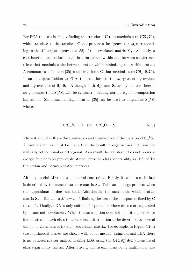
76 5.1 Introduction
For PCA the cost is simply finding the transform C that maximises tr(CΣYC′),
which translates to the transform C that preserves the eigenvectors φi correspond-
ing to the M largest eigenvalues [35] of the covariance matrix ΣY. Similarly, a
cost function can be formulated in terms of the within and between scatter ma-
trices that maximises the between scatter while minimising the within scatter.
A common cost function [35] is the transform C that maximises tr(CS−1w SbC
′).
In an analagous fashion to PCA, this translates to the M greatest eigenvalues
and eigenvectors of S−1w Sb. Although both S−1
w and Sb are symmetric there is
no guarantee that S−1w Sb will be symmetric making normal eigen-decompostion
impossible. Simultaneous diagonilsation [35] can be used to diagonilise S−1w Sb
where,
C′S−1w C = I and C′SbC = Λ (5.11)
where Λ and C = Φ are the eigenvalues and eigenvectors of the matrices of S−1w Sb.
A cautionary note must be made that the resulting eigenvectors in C are not
mutually orthonormal or orthogonal. As a result the transform does not preserve
energy, but does as previously stated, preserve class separability as defined by
the within and between scatter matrices.
Although useful LDA has a number of constraints. Firstly, it assumes each class
is described by the same covariance matrix Sb. This can be large problem when
this approximation does not hold. Additionally, the rank of the within scatter
matrix Sw is limited to M <= L−1 limiting the size of the subspace defined by C
to L− 1. Finally, LDA is only suitable for problems where classes are separated
by means not covariances. When this assumption does not hold it is possible to
find clusters in each class that force each distribution to be described by several
unimodal Gaussians of the same covariance matrix. For example, in Figure 5.2(a)
two multimodal classes are shown with equal means. Using normal LDA there
is no between scatter matrix, making LDA using the tr(CS−1w SbC
′) measure of
class separability useless. Alternatively, due to each class being multimodal, the
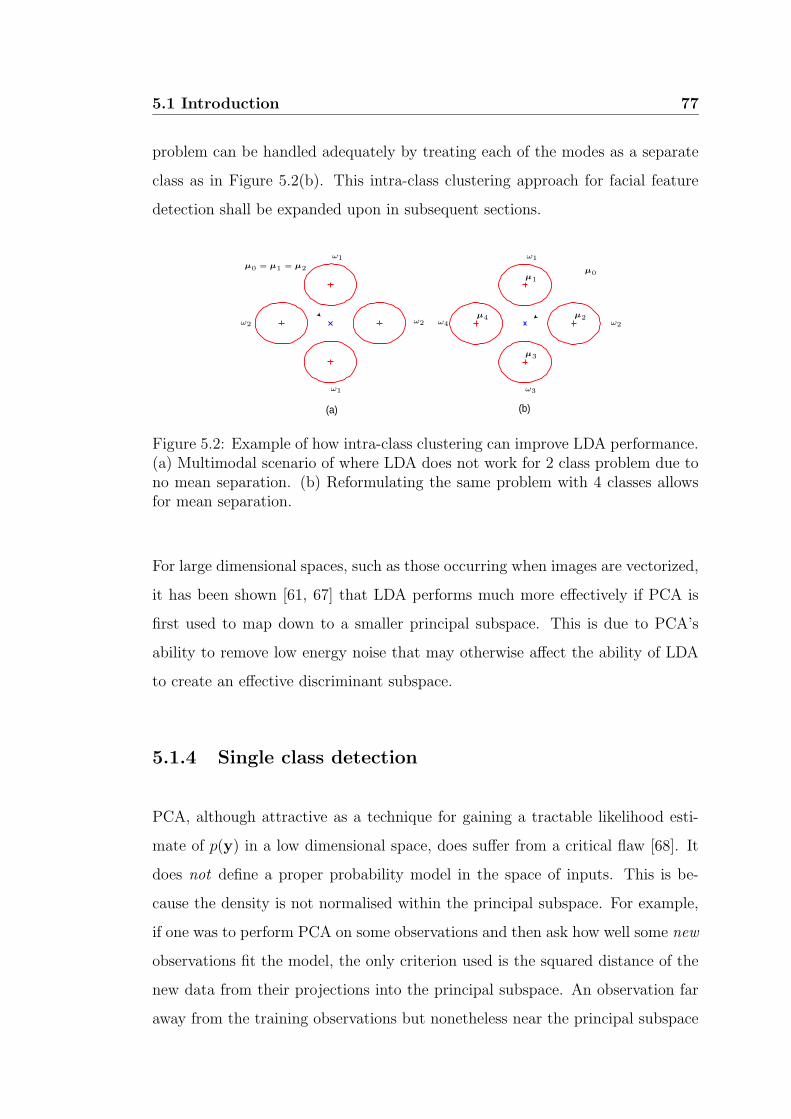
5.1 Introduction 77
problem can be handled adequately by treating each of the modes as a separate
class as in Figure 5.2(b). This intra-class clustering approach for facial feature
detection shall be expanded upon in subsequent sections.
(a) (b)
PSfrag replacements
ω1
ω1
ω1
ω2ω2ω2
ω3
ω4
µ0 = µ1 = µ2
µ1
µ2
µ3
µ4
µ0
Figure 5.2: Example of how intra-class clustering can improve LDA performance.(a) Multimodal scenario of where LDA does not work for 2 class problem due tono mean separation. (b) Reformulating the same problem with 4 classes allowsfor mean separation.
For large dimensional spaces, such as those occurring when images are vectorized,
it has been shown [61, 67] that LDA performs much more effectively if PCA is
first used to map down to a smaller principal subspace. This is due to PCA’s
ability to remove low energy noise that may otherwise affect the ability of LDA
to create an effective discriminant subspace.
5.1.4 Single class detection
PCA, although attractive as a technique for gaining a tractable likelihood esti-
mate of p(y) in a low dimensional space, does suffer from a critical flaw [68]. It
does not define a proper probability model in the space of inputs. This is be-
cause the density is not normalised within the principal subspace. For example,
if one was to perform PCA on some observations and then ask how well some new
observations fit the model, the only criterion used is the squared distance of the
new data from their projections into the principal subspace. An observation far
away from the training observations but nonetheless near the principal subspace
78 5.1 Introduction
will be assigned a high ‘pseudo-likelihood’ or low error. For detection purposes
this can have dire consequences if one needs to detect an object using a single
hypothesis test [35]. This is a common problem where the object class is well
defined but the background class is not. This scenario can best be expressed as,
l1(y)
ωbck
≶
ωobj
Th, l1(y) = log [p(y|λobj)] (5.12)
where l1(y) is a score that discriminates between the object and background class
with Th being the threshold for the decision. In this scenario an object, which is
drastically different in the true observation space, may be considered similar in the
principal subspace or, as it will be referred to in this section, the object space (OS).
This problem can be somewhat resolved by developing a likelihood function that
describes both object space and its complementary residual space (RS). Residual
space is referred to as the complementary subspace that is not spanned by the
object space. Usually, this subspace cannot be computed directly, but a simplistic
measure of its influence can be computed indirectly in terms of the reconstruction
error realised from mapping y into object space. Residual space representations
have proven exceptionally useful in single hypothesis face detection. The success
of residual space representations in a single hypothesis can be realised in terms
of energy. PCA naturally preserves the major modes of variance for an object
in object space. Due to the background class not being defined, any residual
variance can be assumed to stem from non-object variations. Using this logic,
objects with low reconstruction errors can be thought more likely to stem from an
object class rather than background class. Initial work by Turk and Pentland [38],
used just the residual space, as opposed to object space representation for face
detection, as it gave superior results.
A number of approaches have been devised to gain a model to incorporate object
and residual space representations [37, 38, 39, 68, 69, 71] into p(y|λ). Moghaddam
5.1 Introduction 79
and Pentland [39], provided a framework for generating an improved represen-
tation of p(y|λ). In their work they expressed the likelihood function p(y|λ) in
terms of two independent Gaussian densities describing the object and residual
spaces respectively.
p(y|λOS+RS) = p(y|λOS)p(y|λRS) (5.13)
where,
p(y|λOS) = N (0(M×1),Λ(M×M))|x, x = Φ′y (5.14)
p(y|λRS) = N (0([R−M ]×1), σ2I([R−M ]×[R−M ]))|x, x = Φ
′y (5.15)
such that Φ = φiMi=1 are the eigenvectors spanning the subspace corresponding
to the M largest eigenvalues λi, with Φ = φiRi=M+1 being the eigenvectors
spanning the residual subspace. The evaluation of Equation 5.14 is rudimentary
as it simply requires a mapping of y into the object subspace Φ. However,
the evaluation of Equation 5.15 is a little more difficult as one usually does not
have access to the residual subspace Φ to calculate x. Fortunately, one can take
advantage of the complementary nature of object space and the full observation
space such that,
tr(Y′Y) = tr(Λ) + σ2tr(I) (5.16)
so that,
σ2 =[tr(Y′Y) − tr(Λ)]
R−M(5.17)
80 5.1 Introduction
allowing one to rewrite Equation 5.15 as,
p(y|λRS) =exp(− ε2(y)
2σ2 )
(2πσ2)(R−M)/2, ε(y) = y′y − y′ΦΦ′y (5.18)
where ε(y) can be considered as the error in reconstructing y from x. This
equivalence is possible due to the assumption of p(y|λRS) being described by
a Gaussian homoscedastic distribution (i.e. covariance matrix is described by
an isotropic covariance σ2I). This simplistic isotropic representation of residual
space is effective, as the lack of training observations makes any other type of
representation error prone. The problem in this approach is to know the actual
rank of the covariance matrix ΣY describing object space. Empirically, object
space was found to have a rank of approximately R = 50 for the mouth and eye
sub-images experimented upon.
Moghaddam and Pentland [39] calculated their estimate of σ2 differently. They
assumed the first N eigenvalues calculated from the sample covariance matrix
were equivalent to the true eigenvalues for the true rank D covariance matrix
(i.e. if there was an unlimited number of training sub-images), assuming the
eigenspectrum was approximately described by a 1/x function, they were able to
predict the remaining unknown D − N eigenvalues through extrapolation such
that,
σ2 =1
R−N
R∑
i=N+1
λi (5.19)
where R = D. Cootes et al. [59] in a similar decomposition into object and
residual space used an ad-hoc parameter values of σ2 = 12λN+1. For facial feature
detection it was found empirically this last approach performed best.
Many previous papers [39, 69, 70] have shown that objects with complex vari-
ations such as the mouth or eyes do not obey a unimodal distribution in their
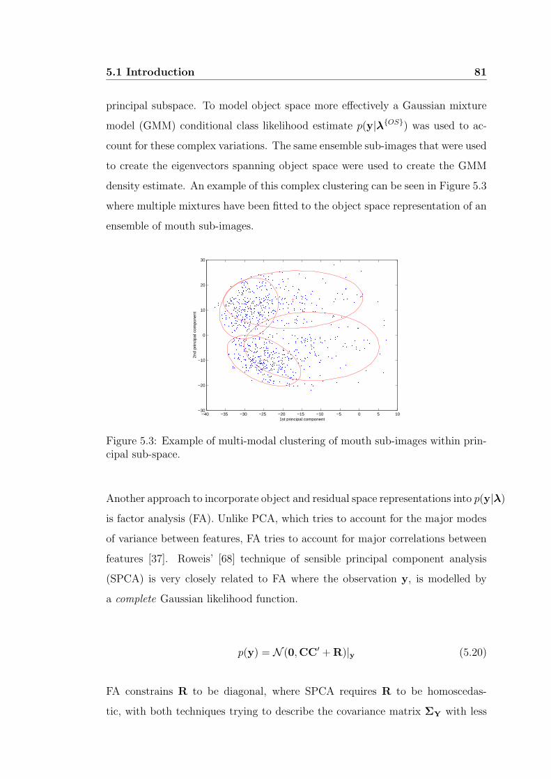
5.1 Introduction 81
principal subspace. To model object space more effectively a Gaussian mixture
model (GMM) conditional class likelihood estimate p(y|λOS) was used to ac-
count for these complex variations. The same ensemble sub-images that were used
to create the eigenvectors spanning object space were used to create the GMM
density estimate. An example of this complex clustering can be seen in Figure 5.3
where multiple mixtures have been fitted to the object space representation of an
ensemble of mouth sub-images.
−40 −35 −30 −25 −20 −15 −10 −5 0 5 10−30
−20
−10
0
10
20
30
1st principal component
2nd
prin
cipa
l com
pone
nt
Figure 5.3: Example of multi-modal clustering of mouth sub-images within prin-cipal sub-space.
Another approach to incorporate object and residual space representations into p(y|λ)
is factor analysis (FA). Unlike PCA, which tries to account for the major modes
of variance between features, FA tries to account for major correlations between
features [37]. Roweis’ [68] technique of sensible principal component analysis
(SPCA) is very closely related to FA where the observation y, is modelled by
a complete Gaussian likelihood function.
p(y) = N (0,CC′ + R)|y (5.20)
FA constrains R to be diagonal, where SPCA requires R to be homoscedas-
tic, with both techniques trying to describe the covariance matrix ΣY with less
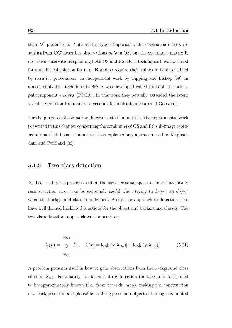
82 5.1 Introduction
than D2 parameters. Note in this type of approach, the covariance matrix re-
sulting from CC′ describes observations only in OS, but the covariance matrix R
describes observations spanning both OS and RS. Both techniques have no closed
form analytical solution for C or R and so require their values to be determined
by iterative procedures. In independent work by Tipping and Bishop [69] an
almost equivalent technique to SPCA was developed called probabilistic princi-
pal component analysis (PPCA). In this work they actually extended the latent
variable Gaussian framework to account for multiple mixtures of Gaussians.
For the purposes of comparing different detection metrics, the experimental work
presented in this chapter concerning the combining of OS and RS sub-image repre-
sentations shall be constrained to the complementary approach used by Moghad-
dam and Pentland [39].
5.1.5 Two class detection
As discussed in the previous section the use of residual space, or more specifically
reconstruction error, can be extremely useful when trying to detect an object
when the background class is undefined. A superior approach to detection is to
have well defined likelihood functions for the object and background classes. The
two class detection approach can be posed as,
l2(y) =
ωbck
≶
ωobj
Th, l2(y) = log[p(y|λobj)] − log[p(y|λbck)] (5.21)
A problem presents itself in how to gain observations from the background class
to train λbck. Fortunately, for facial feature detection the face area is assumed
to be approximately known (i.e. from the skin map), making the construction
of a background model plausible as the type of non-object sub-images is limited
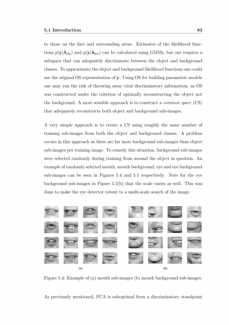
5.1 Introduction 83
to those on the face and surrounding areas. Estimates of the likelihood func-
tions p(y|λobj) and p(y|λbck) can be calculated using GMMs, but one requires a
subspace that can adequately discriminate between the object and background
classes. To approximate the object and background likelihood functions one could
use the original OS representation of y. Using OS for building parametric models
one may run the risk of throwing away vital discriminatory information, as OS
was constructed under the criterion of optimally reconstructing the object not
the background. A more sensible approach is to construct a common space (CS)
that adequately reconstructs both object and background sub-images.
A very simple approach is to create a CS using roughly the same number of
training sub-images from both the object and background classes. A problem
occurs in this approach as there are far more background sub-images than object
sub-images per training image. To remedy this situation, background sub-images
were selected randomly during training from around the object in question. An
example of randomly selected mouth, mouth background, eye and eye background
sub-images can be seen in Figures 5.4 and 5.5 respectively. Note for the eye
background sub-images in Figure 5.5(b) that the scale varies as well. This was
done to make the eye detector robust to a multi-scale search of the image.
(a) (b)
Figure 5.4: Example of (a) mouth sub-images (b) mouth background sub-images.
As previously mentioned, PCA is suboptimal from a discriminatory standpoint
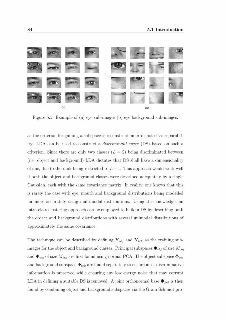
84 5.1 Introduction
(a) (b)
Figure 5.5: Example of (a) eye sub-images (b) eye background sub-images.
as the criterion for gaining a subspace is reconstruction error not class separabil-
ity. LDA can be used to construct a discriminant space (DS) based on such a
criterion. Since there are only two classes (L = 2) being discriminated between
(i.e. object and background) LDA dictates that DS shall have a dimensionality
of one, due to the rank being restricted to L− 1. This approach would work well
if both the object and background classes were described adequately by a single
Gaussian, each with the same covariance matrix. In reality, one knows that this
is rarely the case with eye, mouth and background distributions being modelled
far more accurately using multimodal distributions. Using this knowledge, an
intra-class clustering approach can be employed to build a DS by describing both
the object and background distributions with several unimodal distributions of
approximately the same covariance.
The technique can be described by defining Yobj and Ybck as the training sub-
images for the object and background classes. Principal subspaces Φobj of sizeMobj
and Φbck of size Mbck are first found using normal PCA. The object subspace Φobj
and background subspace Φbck are found separately to ensure most discriminative
information is preserved while ensuring any low energy noise that may corrupt
LDA in defining a suitable DS is removed. A joint orthonormal base Φjnt is then
found by combining object and background subspaces via the Gram-Schmidt pro-
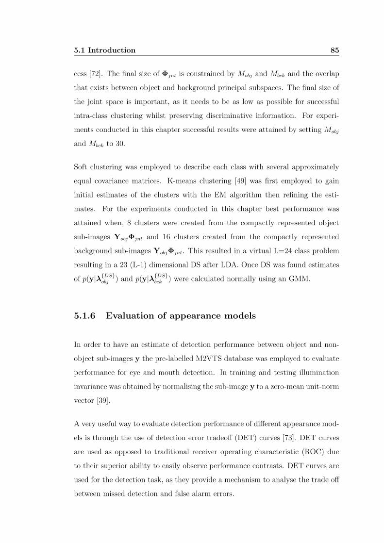
5.1 Introduction 85
cess [72]. The final size of Φjnt is constrained by Mobj and Mbck and the overlap
that exists between object and background principal subspaces. The final size of
the joint space is important, as it needs to be as low as possible for successful
intra-class clustering whilst preserving discriminative information. For experi-
ments conducted in this chapter successful results were attained by setting Mobj
and Mbck to 30.
Soft clustering was employed to describe each class with several approximately
equal covariance matrices. K-means clustering [49] was first employed to gain
initial estimates of the clusters with the EM algorithm then refining the esti-
mates. For the experiments conducted in this chapter best performance was
attained when, 8 clusters were created from the compactly represented object
sub-images YobjΦjnt and 16 clusters created from the compactly represented
background sub-images YobjΦjnt. This resulted in a virtual L=24 class problem
resulting in a 23 (L-1) dimensional DS after LDA. Once DS was found estimates
of p(y|λDSobj ) and p(y|λDS
bck ) were calculated normally using an GMM.
5.1.6 Evaluation of appearance models
In order to have an estimate of detection performance between object and non-
object sub-images y the pre-labelled M2VTS database was employed to evaluate
performance for eye and mouth detection. In training and testing illumination
invariance was obtained by normalising the sub-image y to a zero-mean unit-norm
vector [39].
A very useful way to evaluate detection performance of different appearance mod-
els is through the use of detection error tradeoff (DET) curves [73]. DET curves
are used as opposed to traditional receiver operating characteristic (ROC) due
to their superior ability to easily observe performance contrasts. DET curves are
used for the detection task, as they provide a mechanism to analyse the trade off
between missed detection and false alarm errors.

86 5.1 Introduction
Results are presented here for the following detection metrics,
OS-L1 Object space representation of y for the single hypothesis score l1(y)
where p(y|λOSobj ) is approximated by an 8 mixture diagonal GMM. OS is
an 30 dimensional space.
OS-L2 Object space representation of y for the two class hypothesis score l2(y)
where p(y|λOSobj ) is an 8 mixture diagonal GMM and p(y|λOS
bck ) is an 16
mixture diagonal GMM. OS is an 30 dimensional space.
RS-L1 Residual space representation of y for the single hypothesis score l1(y)
where p(y|λRSobj ) is parametrically by single mixture isotropic Gaussian.
The OS used to gain the RS metric was an 5 dimensional space.
OS+RS-L1 Complementary object and residual space representation of y for
the single hypothesis score l1(y) where p(y|λOS+RSobj ) = p(y|λOS
obj )p(y|λRSobj ).
The likelihood function p(y|λOSobj ) is parametrically described by an 8 mix-
ture diagonal GMM, with p(y|λRSobj ) being described by single mixture
isotropic Gaussian. OS is an 5 dimensional space.
CS-L2 Common space representation of y for the two class hypothesis score l2(y)
where p(y|λCSobj ) is an 8 mixture diagonal GMM and p(y|λCS
bck ) is an 16
mixture diagonal GMM. CS is an 30 dimensional space.
DS-L2 Discriminant space representation of y for the two class hypothesis score l2(y)
where p(y|λDSobj ) is an 8 mixture diagonal GMM and p(y|λDS
bck ) is an 16
mixture diagonal GMM. DS is an 23 dimensional space.
The same GMM topologies were found to be effective for both mouth and eye
detection. In all cases, classifiers were trained using images from shot 1 of the
M2VTS database with testing being performed on shots 2 and 3. To generate
DET curves for eye and mouth detection, 30 random background sub-images
were extracted for every object sub-image. In testing this resulted in over 5000
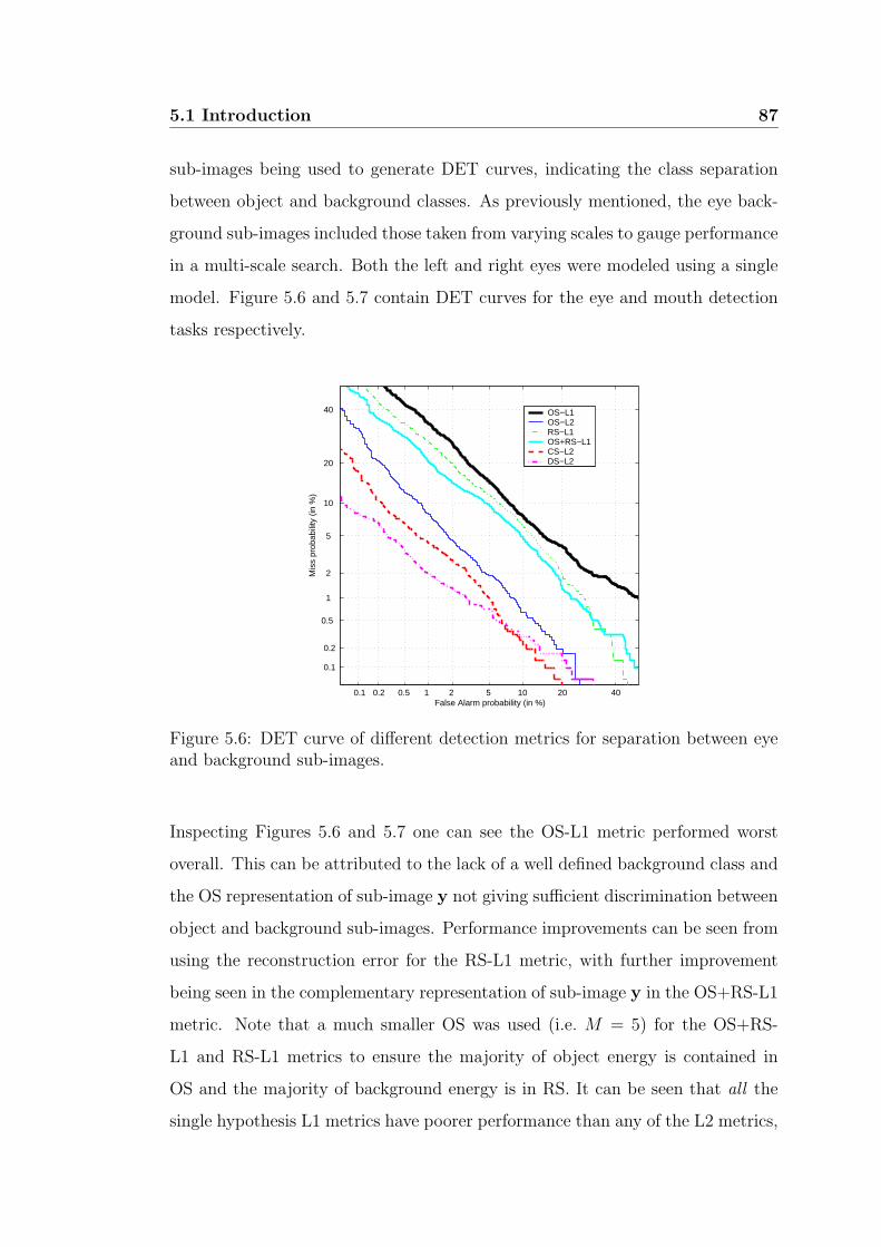
5.1 Introduction 87
sub-images being used to generate DET curves, indicating the class separation
between object and background classes. As previously mentioned, the eye back-
ground sub-images included those taken from varying scales to gauge performance
in a multi-scale search. Both the left and right eyes were modeled using a single
model. Figure 5.6 and 5.7 contain DET curves for the eye and mouth detection
tasks respectively.
0.1 0.2 0.5 1 2 5 10 20 40
0.1
0.2
0.5
1
2
5
10
20
40
False Alarm probability (in %)
Mis
s pr
obab
ility
(in
%)
OS−L1 OS−L2 RS−L1 OS+RS−L1CS−L2 DS−L2
Figure 5.6: DET curve of different detection metrics for separation between eyeand background sub-images.
Inspecting Figures 5.6 and 5.7 one can see the OS-L1 metric performed worst
overall. This can be attributed to the lack of a well defined background class and
the OS representation of sub-image y not giving sufficient discrimination between
object and background sub-images. Performance improvements can be seen from
using the reconstruction error for the RS-L1 metric, with further improvement
being seen in the complementary representation of sub-image y in the OS+RS-L1
metric. Note that a much smaller OS was used (i.e. M = 5) for the OS+RS-
L1 and RS-L1 metrics to ensure the majority of object energy is contained in
OS and the majority of background energy is in RS. It can be seen that all the
single hypothesis L1 metrics have poorer performance than any of the L2 metrics,
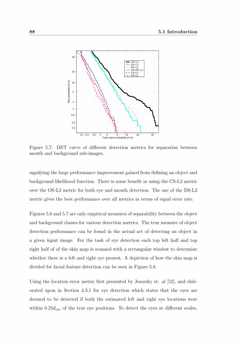
88 5.1 Introduction
0.1 0.2 0.5 1 2 5 10 20 40
0.1
0.2
0.5
1
2
5
10
20
40
False Alarm probability (in %)
Mis
s pr
obab
ility
(in
%)
OS−L1 OS−L2 RS−L1 OS+RS−L1CS−L2 DS−L2
Figure 5.7: DET curve of different detection metrics for separation betweenmouth and background sub-images.
signifying the large performance improvement gained from defining an object and
background likelihood function. There is some benefit in using the CS-L2 metric
over the OS-L2 metric for both eye and mouth detection. The use of the DS-L2
metric gives the best performance over all metrics in terms of equal error rate.
Figures 5.6 and 5.7 are only empirical measures of separability between the object
and background classes for various detection metrics. The true measure of object
detection performance can be found in the actual act of detecting an object in
a given input image. For the task of eye detection each top left half and top
right half of of the skin map is scanned with a rectangular window to determine
whether there is a left and right eye present. A depiction of how the skin map is
divided for facial feature detection can be seen in Figure 5.8.
Using the location error metric first presented by Jesorsky et. al [52], and elab-
orated upon in Section 4.3.1 for eye detection which states that the eyes are
deemed to be detected if both the estimated left and right eye locations were
within 0.25deye of the true eye positions. To detect the eyes at different scales,
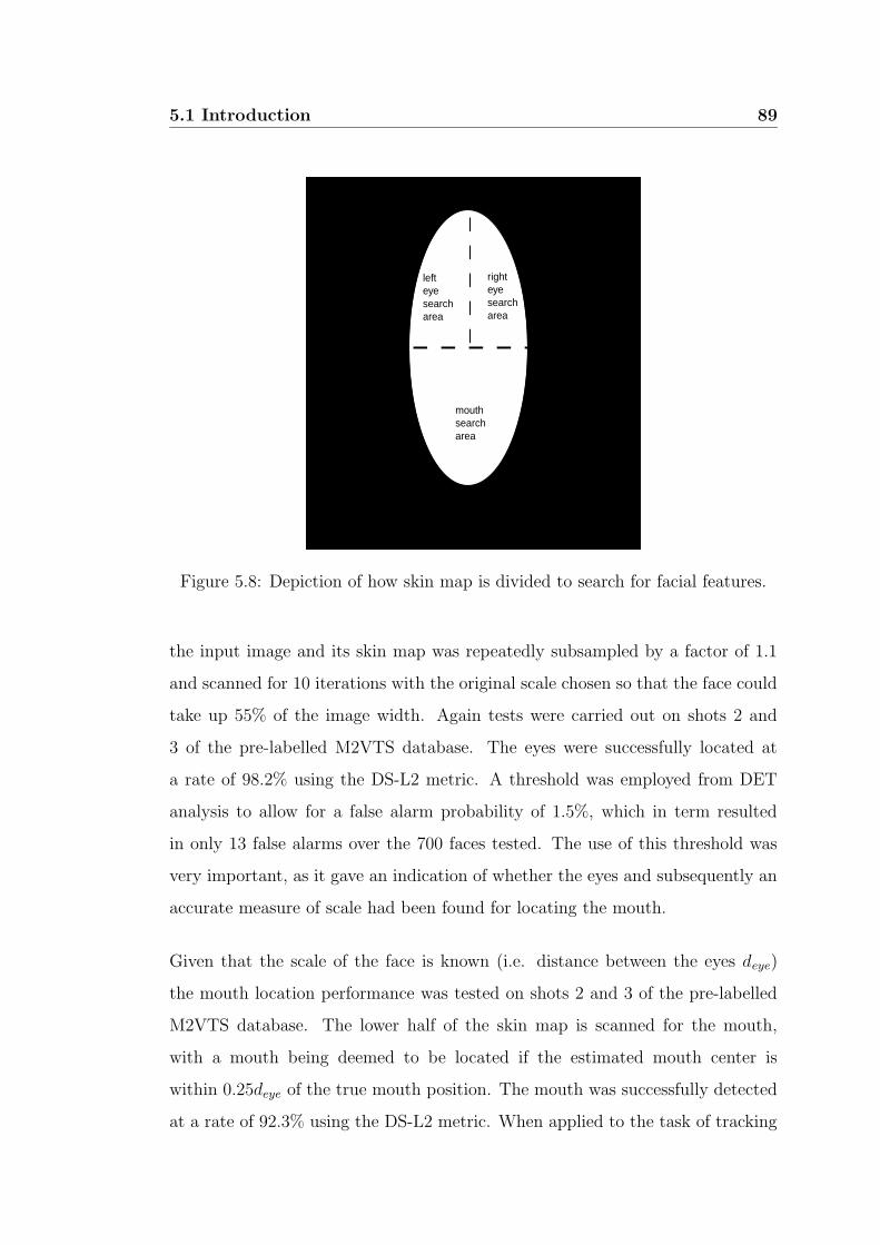
5.1 Introduction 89
right eye search area
left eye search area
mouth search area
Figure 5.8: Depiction of how skin map is divided to search for facial features.
the input image and its skin map was repeatedly subsampled by a factor of 1.1
and scanned for 10 iterations with the original scale chosen so that the face could
take up 55% of the image width. Again tests were carried out on shots 2 and
3 of the pre-labelled M2VTS database. The eyes were successfully located at
a rate of 98.2% using the DS-L2 metric. A threshold was employed from DET
analysis to allow for a false alarm probability of 1.5%, which in term resulted
in only 13 false alarms over the 700 faces tested. The use of this threshold was
very important, as it gave an indication of whether the eyes and subsequently an
accurate measure of scale had been found for locating the mouth.
Given that the scale of the face is known (i.e. distance between the eyes deye)
the mouth location performance was tested on shots 2 and 3 of the pre-labelled
M2VTS database. The lower half of the skin map is scanned for the mouth,
with a mouth being deemed to be located if the estimated mouth center is
within 0.25deye of the true mouth position. The mouth was successfully detected
at a rate of 92.3% using the DS-L2 metric. When applied to the task of tracking
90 5.2 Chapter Summary
in a continuous video sequence, this location rate starts approaching 100% due
to the smoothing of the mouth coordinates through time via a median filter.
5.2 Chapter Summary
Appearance based detection of the eyes and mouth is of real benefit in AVSP
applications. The appearance based paradigm allows for detection, not just loca-
tion, which is essential for effective AVSP applications. A number of techniques
have been evaluated for the task of appearance based eye and mouth detection.
All techniques differ primarily in their representation of the sub-image y be-
ing evaluated and how an appropriate likelihood score is generated. Techniques
based on single class detection (similarity measure based solely on the object)
have been shown to be inferior to those generated from two class detection (sim-
ilarity measure based on both the object and background classes). Similarly, the
need for gaining a compact representation of the sub-image y that is discrimina-
tory between the mouth and background is beneficial, as opposed to approaches
that generate a compact representation of the object or both classes based on
reconstruction error.
A technique for creating a compact discriminant space has been outlined using
knowledge of LDA’s criterion for class separation. In this approach an intra-
class clustering approach is employed to handle the typical case of when both the
object and background class distributions are multimodal. Using this approach
good results, suitable for use in AVSP, were achieved in practice for the tasks of
eye detection and mouth location/tracking.
Chapter 6
Feature Invariant Lip
Location/Tracking
6.1 Introduction
Feature invariant lip location/tracking pertains to the fitting of a labial contour
model to a mouth image. The feature invariant location/tracking paradigm, as
previously discussed in Chapter 4, tries to find structural components of the lips
that are invariant to changes in position, scale and shape. There has been a
plethora of work done in feature invariant lip location/tracking [4, 57, 58]. The
term lip location, rather than mouth location, is used here as these techniques
locate the outer, and sometimes inner, labial contour of the mouth from which
the mouth center is then deduced. An additional benefit of this type of approach
is that the resultant labial contour describing the mouth shape can be used as
an additional feature in an AVSP application. The task of feature invariant lip
location can be broken into two tasks namely,
1. the generation of a potential map f(x, y) signifying the likelihood of the lip
shape model’s boundary lying at the pixel coordinates (x, y), and
92 6.1 Introduction
2. the fitting of the lip shape model λg to the potential image f(x, y).
The first problem of generating the ‘potential image’/‘edge-map’ (ie. a binary
image describing the outline of an object) f(x, y) can be posed as,
f(x, y) =
1 TRGB(x, y)
0 else(6.1)
where T is some edge enhancement operator, and RGB(x, y) is the original colour
image. The second problem pertaining to the extraction of the labial contour
from the potential image f(x, y) has to be performed in a manner that has low
sensitivity to the initialisation of the estimated contour and any noisy artifacts
present in the potential image.
This chapter is broken down into two major parts. Firstly, Sections 6.2 to 6.5
discuss the generation of the potential map f(x, y) through image segmentation,
in particular chromatic segmentation. A soft clustering approach is employed to
automatically deduce the lip and background distributions from samples of pixels
taken from a subject’s mouth region of interest (ROI) using a maximum likelihood
criteria. Results are presented that can segment a subject’s lips from its back-
ground with no a priori knowledge except the use of the initial starting clusters
for the lip and background classes. The M2VTS [2] database is used to present
results for unsupervised mouth segmentation over a wide number of subjects. The
second part of this chapter (Sections 6.6 to 6.11) investigates the problem of how
to fit a parametric lip shape model λg to the potential image f(x, y), and what
parametric form λg should take on. Results are presented in terms of correctly
found mouth centers using the M2VTS database.
6.2 Lip Segmentation 93
6.2 Lip Segmentation
Segmentation is a common approach in computer vision to track the outline or
shape of an object. However, with such an approach the accuracy or usefulness of
the tracked object is directly related to how well the object has been segmented
from its background. Segmentation of the lips from its facial background is a
very difficult problem due to the low grayscale variation around the mouth [57].
Chromatic pixel based features have shown to be useful for segmenting a person’s
lips from the primarily skin background [57, 58, 62, 63]. Such techniques take
advantage of the premise that lips pixels are much redder than the paler skin
background pixels that they coexist with.
However, using colour as a feature has several problems. Firstly, the colour rep-
resentation of a person obtained by a camera is influenced by ambient light and
background. Secondly, different cameras produce significantly different colour
values, even for the same person under the same lighting conditions [54]. Finally,
the class models describing the chromatic distribution of pixels in both the mouth
and background classes can vary from person to person. All these effects can be
grouped together under the banner of a problem known in computer vision circles
as colour constancy. Colour constancy refers to the ability to identify a surface
as having the same colour under considerably different viewing conditions. The
colour constancy problem requires a classifier, using chrominance as a feature for
segmentation, to be as adaptive as possible. The term adaptive lip segmenta-
tion is used in this chapter to describe the task of segmenting the lips from the
surrounding skin background in an unsupervised manner such that an a priori
parametric description of either class is not required.
The problem of low grayscale distinction between the mouth and its background
has been previously addressed by a deformable template paradigm, as previously
discussed in Chapter 4. In this paradigm a priori knowledge of the mouth’s shape
and texture is incorporated into an adaptive high dimensional energy minimisa-
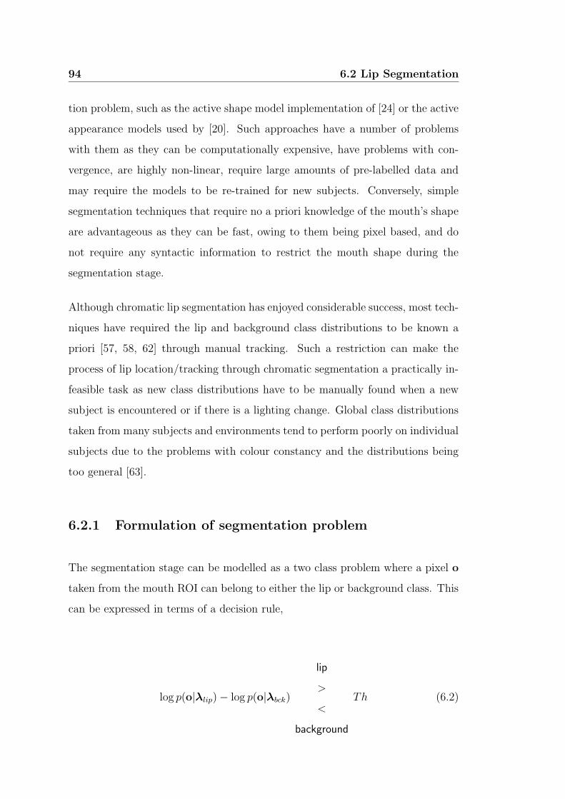
94 6.2 Lip Segmentation
tion problem, such as the active shape model implementation of [24] or the active
appearance models used by [20]. Such approaches have a number of problems
with them as they can be computationally expensive, have problems with con-
vergence, are highly non-linear, require large amounts of pre-labelled data and
may require the models to be re-trained for new subjects. Conversely, simple
segmentation techniques that require no a priori knowledge of the mouth’s shape
are advantageous as they can be fast, owing to them being pixel based, and do
not require any syntactic information to restrict the mouth shape during the
segmentation stage.
Although chromatic lip segmentation has enjoyed considerable success, most tech-
niques have required the lip and background class distributions to be known a
priori [57, 58, 62] through manual tracking. Such a restriction can make the
process of lip location/tracking through chromatic segmentation a practically in-
feasible task as new class distributions have to be manually found when a new
subject is encountered or if there is a lighting change. Global class distributions
taken from many subjects and environments tend to perform poorly on individual
subjects due to the problems with colour constancy and the distributions being
too general [63].
6.2.1 Formulation of segmentation problem
The segmentation stage can be modelled as a two class problem where a pixel o
taken from the mouth ROI can belong to either the lip or background class. This
can be expressed in terms of a decision rule,
log p(o|λlip) − log p(o|λbck)
lip
>
<
background
Th (6.2)
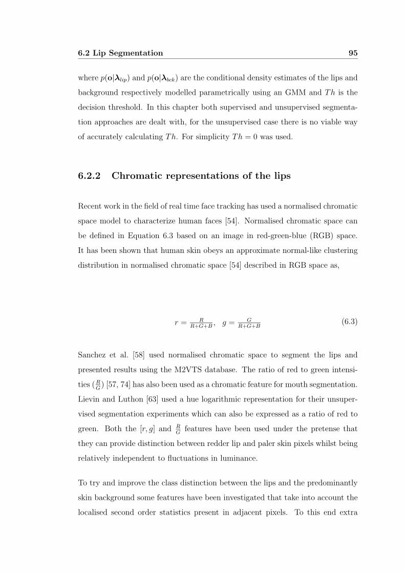
6.2 Lip Segmentation 95
where p(o|λlip) and p(o|λbck) are the conditional density estimates of the lips and
background respectively modelled parametrically using an GMM and Th is the
decision threshold. In this chapter both supervised and unsupervised segmenta-
tion approaches are dealt with, for the unsupervised case there is no viable way
of accurately calculating Th. For simplicity Th = 0 was used.
6.2.2 Chromatic representations of the lips
Recent work in the field of real time face tracking has used a normalised chromatic
space model to characterize human faces [54]. Normalised chromatic space can
be defined in Equation 6.3 based on an image in red-green-blue (RGB) space.
It has been shown that human skin obeys an approximate normal-like clustering
distribution in normalised chromatic space [54] described in RGB space as,
r = RR+G+B
, g = GR+G+B
(6.3)
Sanchez et al. [58] used normalised chromatic space to segment the lips and
presented results using the M2VTS database. The ratio of red to green intensi-
ties (RG) [57, 74] has also been used as a chromatic feature for mouth segmentation.
Lievin and Luthon [63] used a hue logarithmic representation for their unsuper-
vised segmentation experiments which can also be expressed as a ratio of red to
green. Both the [r, g] and RG
features have been used under the pretense that
they can provide distinction between redder lip and paler skin pixels whilst being
relatively independent to fluctuations in luminance.
To try and improve the class distinction between the lips and the predominantly
skin background some features have been investigated that take into account the
localised second order statistics present in adjacent pixels. To this end extra
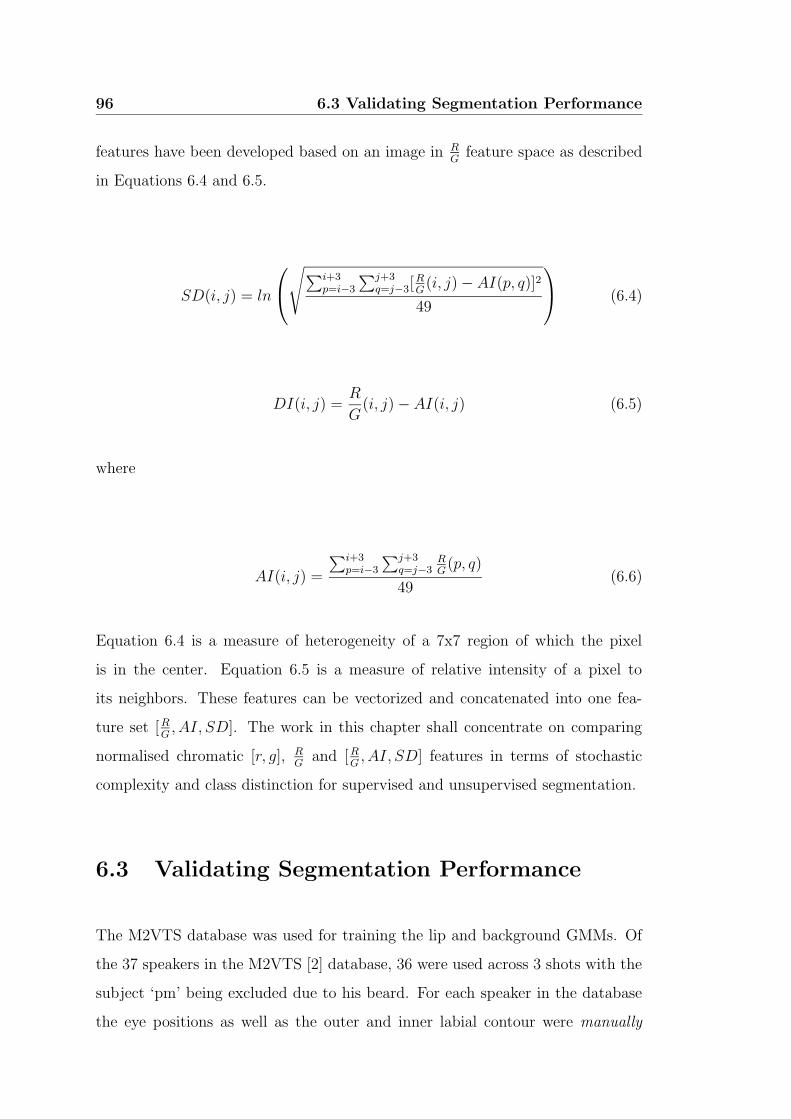
96 6.3 Validating Segmentation Performance
features have been developed based on an image in RG
feature space as described
in Equations 6.4 and 6.5.
SD(i, j) = ln
√∑i+3
p=i−3
∑j+3q=j−3[
RG(i, j) − AI(p, q)]2
49
(6.4)
DI(i, j) =R
G(i, j) − AI(i, j) (6.5)
where
AI(i, j) =
∑i+3p=i−3
∑j+3q=j−3
RG(p, q)
49(6.6)
Equation 6.4 is a measure of heterogeneity of a 7x7 region of which the pixel
is in the center. Equation 6.5 is a measure of relative intensity of a pixel to
its neighbors. These features can be vectorized and concatenated into one fea-
ture set [RG, AI, SD]. The work in this chapter shall concentrate on comparing
normalised chromatic [r, g], RG
and [RG, AI, SD] features in terms of stochastic
complexity and class distinction for supervised and unsupervised segmentation.
6.3 Validating Segmentation Performance
The M2VTS database was used for training the lip and background GMMs. Of
the 37 speakers in the M2VTS [2] database, 36 were used across 3 shots with the
subject ‘pm’ being excluded due to his beard. For each speaker in the database
the eye positions as well as the outer and inner labial contour were manually
6.4 Supervised Lip Segmentation 97
tracked from frames 1 to 100 at 10 frame intervals. This resulted in over 1000
pre-tracked frames with approximately 11 pre-tracked frames per subject per
shot. The mouth ROI chosen for segmentation was based on the subject’s eye
separation distance deye, with a (3deye)×(4deye) box centered at the mouth center.
The human trackers, who were asked to manually track the mouth and eyes of the
M2VTS subjects, reported much difficulty in labelling the outer labial contour.
This highlights a fundamental problem associated with mouth location/tracking
as the uncertainty between the skin and mouth regions also suggests why ap-
proaches based on edge finding often fail. Segmentation techniques that treat the
mouth much more like a texture have been more successful. This boundary un-
certainty can be reduced using post-processing that place temporal and syntactic
restrictions on the resultant shape so as to reduce errors from the segmentation
process [27, 57, 62].
The boundary uncertainty also makes it difficult to gain an accurate quantitative
measure of how effective a certain segmentation technique is. The rate of incor-
rectly labelled pixels (i.e. lip or background) in the mouth ROI was used so as
to gain a rough quantitative measure of how well the segmentation process has
gone. Unfortunately, this metric alone cannot be accurately used as poor error
rates can be received from the subject’s mouth being open or nose being seg-
mented along with the lips, even though the lips have been segmented accurately.
To remedy this situation the estimated mouth centers, deduced from the fitting
of a labial contour model to the potential image f(x, y) produced as a result of
segmentation, can be used as an additional indirect measure of performance.
6.4 Supervised Lip Segmentation
Before investigating how to adaptively segment the lips from subject to subject
one has to find which features and classifier topologies perform best given pre-
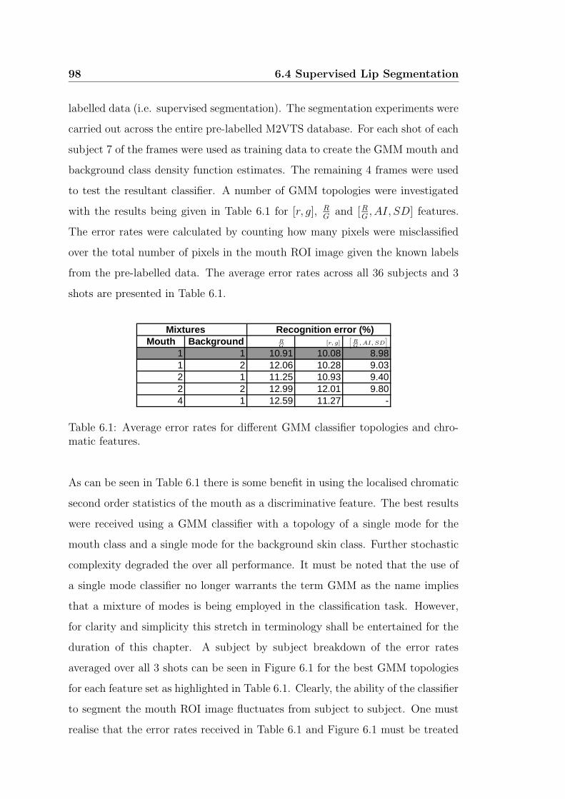
98 6.4 Supervised Lip Segmentation
labelled data (i.e. supervised segmentation). The segmentation experiments were
carried out across the entire pre-labelled M2VTS database. For each shot of each
subject 7 of the frames were used as training data to create the GMM mouth and
background class density function estimates. The remaining 4 frames were used
to test the resultant classifier. A number of GMM topologies were investigated
with the results being given in Table 6.1 for [r, g], RG
and [RG, AI, SD] features.
The error rates were calculated by counting how many pixels were misclassified
over the total number of pixels in the mouth ROI image given the known labels
from the pre-labelled data. The average error rates across all 36 subjects and 3
shots are presented in Table 6.1.
Mixtures Recognition error (%)Mouth Background
1 1 10.91 10.08 8.981 2 12.06 10.28 9.032 1 11.25 10.93 9.402 2 12.99 12.01 9.804 1 12.59 11.27 -
PSfrag replacements
RG
[RG
, AI, SD]
[r, g]
Table 6.1: Average error rates for different GMM classifier topologies and chro-matic features.
As can be seen in Table 6.1 there is some benefit in using the localised chromatic
second order statistics of the mouth as a discriminative feature. The best results
were received using a GMM classifier with a topology of a single mode for the
mouth class and a single mode for the background skin class. Further stochastic
complexity degraded the over all performance. It must be noted that the use of
a single mode classifier no longer warrants the term GMM as the name implies
that a mixture of modes is being employed in the classification task. However,
for clarity and simplicity this stretch in terminology shall be entertained for the
duration of this chapter. A subject by subject breakdown of the error rates
averaged over all 3 shots can be seen in Figure 6.1 for the best GMM topologies
for each feature set as highlighted in Table 6.1. Clearly, the ability of the classifier
to segment the mouth ROI image fluctuates from subject to subject. One must
realise that the error rates received in Table 6.1 and Figure 6.1 must be treated
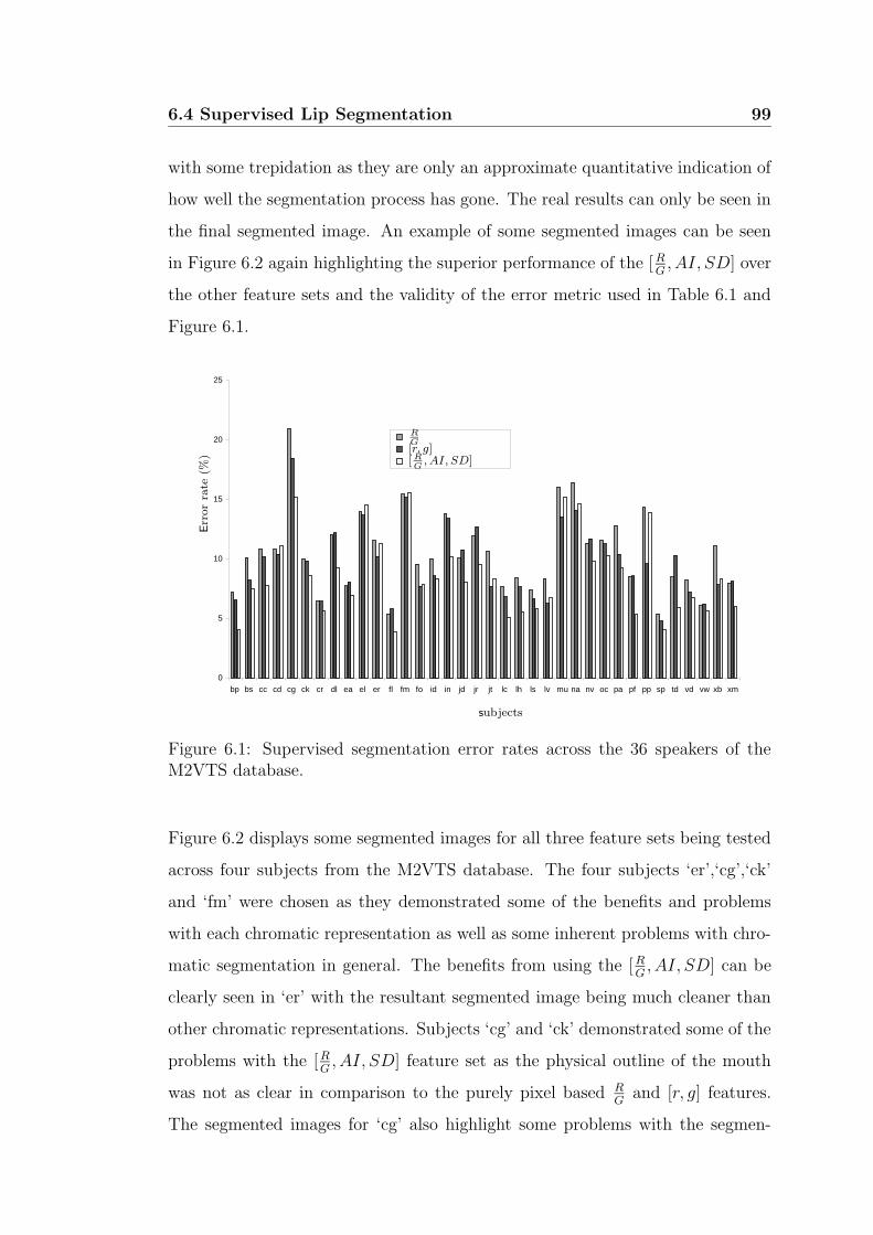
6.4 Supervised Lip Segmentation 99
with some trepidation as they are only an approximate quantitative indication of
how well the segmentation process has gone. The real results can only be seen in
the final segmented image. An example of some segmented images can be seen
in Figure 6.2 again highlighting the superior performance of the [RG, AI, SD] over
the other feature sets and the validity of the error metric used in Table 6.1 and
Figure 6.1.
0
5
10
15
20
25
bp bs cc cd cg ck cr dl ea el er fl fm fo id in jd jr jt lc lh ls lv mu na nv oc pa pf pp sp td vd vw xb xm
PSfrag replacements
Err
or
rate
(%)
subjects
RG[r, g][ RG
, AI, SD]
Figure 6.1: Supervised segmentation error rates across the 36 speakers of theM2VTS database.
Figure 6.2 displays some segmented images for all three feature sets being tested
across four subjects from the M2VTS database. The four subjects ‘er’,‘cg’,‘ck’
and ‘fm’ were chosen as they demonstrated some of the benefits and problems
with each chromatic representation as well as some inherent problems with chro-
matic segmentation in general. The benefits from using the [RG, AI, SD] can be
clearly seen in ‘er’ with the resultant segmented image being much cleaner than
other chromatic representations. Subjects ‘cg’ and ‘ck’ demonstrated some of the
problems with the [RG, AI, SD] feature set as the physical outline of the mouth
was not as clear in comparison to the purely pixel based RG
and [r, g] features.
The segmented images for ‘cg’ also highlight some problems with the segmen-
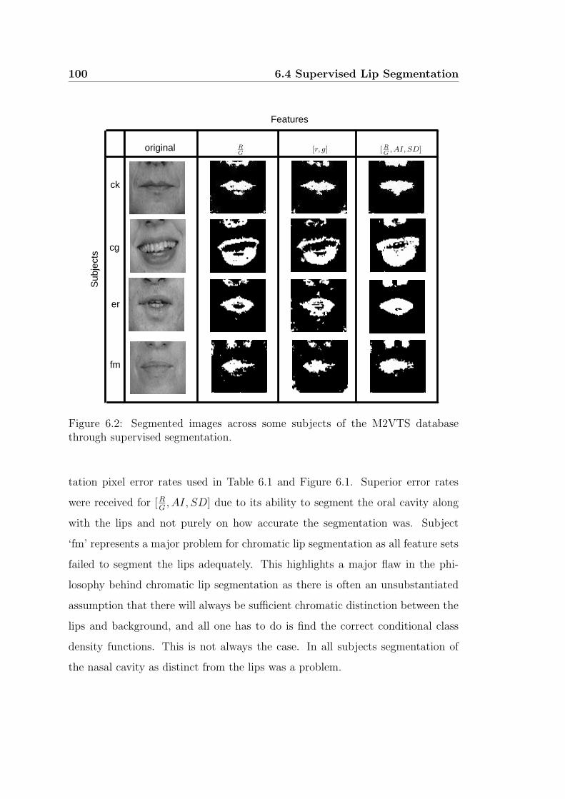
100 6.4 Supervised Lip Segmentation
er
cg
ck
fm
original
Features
Sub
ject
s
PSfrag replacements
RG
[r, g] [ RG
, AI, SD]
Figure 6.2: Segmented images across some subjects of the M2VTS databasethrough supervised segmentation.
tation pixel error rates used in Table 6.1 and Figure 6.1. Superior error rates
were received for [RG, AI, SD] due to its ability to segment the oral cavity along
with the lips and not purely on how accurate the segmentation was. Subject
‘fm’ represents a major problem for chromatic lip segmentation as all feature sets
failed to segment the lips adequately. This highlights a major flaw in the phi-
losophy behind chromatic lip segmentation as there is often an unsubstantiated
assumption that there will always be sufficient chromatic distinction between the
lips and background, and all one has to do is find the correct conditional class
density functions. This is not always the case. In all subjects segmentation of
the nasal cavity as distinct from the lips was a problem.
6.5 Unsupervised Lip Segmentation 101
6.5 Unsupervised Lip Segmentation
The problem of clustering has been well defined and investigated in pattern recog-
nition [35]. Clustering is defined by [35] as the classification of samples without
the aid of a training set. Such a clustering approach is ideal for chromatic mouth
segmentation due to problems with colour constancy and the need for subject by
subject adaptivity as reported by [63]. An important goal of finding clusters is
to decompose a complex distribution into several normal-like distributions. By
expressing a complex distribution through the summation of a several normal-
like distributions the problem of pattern recognition, especially classifier design,
becomes considerably easier. This is the main philosophy behind GMM classi-
fiers. The distinction between the terms class distributions and clusters can often
become ambiguous when one is dealing with clustering techniques. This is due to
the assumption that a cluster or groups of clusters found during the unsupervised
clustering process refers to a real world class (i.e. mouth or background).
The estimation of clusters can be a problem when real world classes overlap.
Unfortunately, this is often the case with chromatic representations of the mouth
and the background class distributions. Most unsupervised clustering algorithms
are either hard or soft clustering. Hard clustering refers to a clustering algorithm
that can only allow a given sample from a data set to belong to one particular
cluster. Conversely, soft clustering allows a given sample from a data set to
belong to multiple clusters. When the distinction between classes is poor, a hard
clustering approach requires samples to be assigned to specific classes even though
in reality there may be a large amount of uncertainty to which cluster the sample
really belongs. This can result in ill formed clusters which can drastically affect
the ability to segment the mouth successfully.
Maximum likelihood (ML) estimation is able to perform a soft clustering such
that there are no definite boundaries between classes. The EM algorithm [46]
was chosen to perform the clustering process due to its ability to cluster via
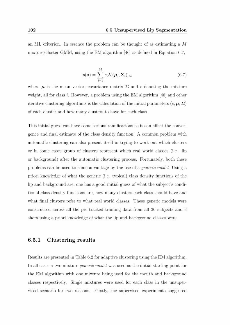
102 6.5 Unsupervised Lip Segmentation
an ML criterion. In essence the problem can be thought of as estimating a M
mixture/cluster GMM, using the EM algorithm [46] as defined in Equation 6.7,
p(o) =M∑
i=1
ciN (µi,Σi)|o, (6.7)
where µ is the mean vector, covariance matrix Σ and c denoting the mixture
weight, all for class i. However, a problem using the EM algorithm [46] and other
iterative clustering algorithms is the calculation of the initial parameters (c,µ,Σ)
of each cluster and how many clusters to have for each class.
This initial guess can have some serious ramifications as it can affect the conver-
gence and final estimate of the class density function. A common problem with
automatic clustering can also present itself in trying to work out which clusters
or in some cases group of clusters represent which real world classes (i.e. lip
or background) after the automatic clustering process. Fortunately, both these
problems can be used to some advantage by the use of a generic model. Using a
priori knowledge of what the generic (i.e. typical) class density functions of the
lip and background are, one has a good initial guess of what the subject’s condi-
tional class density functions are, how many clusters each class should have and
what final clusters refer to what real world classes. These generic models were
constructed across all the pre-tracked training data from all 36 subjects and 3
shots using a priori knowledge of what the lip and background classes were.
6.5.1 Clustering results
Results are presented in Table 6.2 for adaptive clustering using the EM algorithm.
In all cases a two mixture generic model was used as the initial starting point for
the EM algorithm with one mixture being used for the mouth and background
classes respectively. Single mixtures were used for each class in the unsuper-
vised scenario for two reasons. Firstly, the supervised experiments suggested
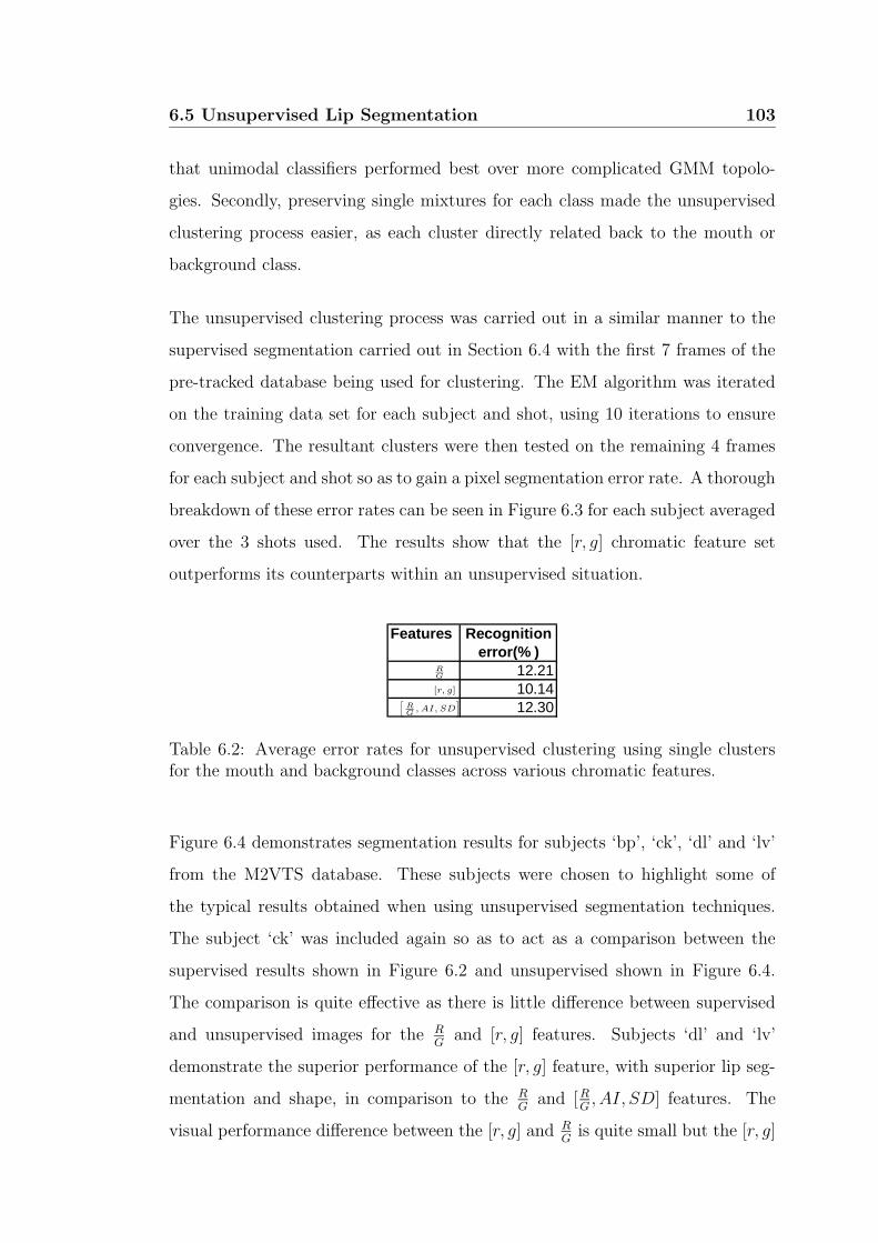
6.5 Unsupervised Lip Segmentation 103
that unimodal classifiers performed best over more complicated GMM topolo-
gies. Secondly, preserving single mixtures for each class made the unsupervised
clustering process easier, as each cluster directly related back to the mouth or
background class.
The unsupervised clustering process was carried out in a similar manner to the
supervised segmentation carried out in Section 6.4 with the first 7 frames of the
pre-tracked database being used for clustering. The EM algorithm was iterated
on the training data set for each subject and shot, using 10 iterations to ensure
convergence. The resultant clusters were then tested on the remaining 4 frames
for each subject and shot so as to gain a pixel segmentation error rate. A thorough
breakdown of these error rates can be seen in Figure 6.3 for each subject averaged
over the 3 shots used. The results show that the [r, g] chromatic feature set
outperforms its counterparts within an unsupervised situation.
Features Recognitionerror(% )
12.2110.1412.30
PSfrag replacements
RG
[RG
, AI, SD]
[r, g]
Table 6.2: Average error rates for unsupervised clustering using single clustersfor the mouth and background classes across various chromatic features.
Figure 6.4 demonstrates segmentation results for subjects ‘bp’, ‘ck’, ‘dl’ and ‘lv’
from the M2VTS database. These subjects were chosen to highlight some of
the typical results obtained when using unsupervised segmentation techniques.
The subject ‘ck’ was included again so as to act as a comparison between the
supervised results shown in Figure 6.2 and unsupervised shown in Figure 6.4.
The comparison is quite effective as there is little difference between supervised
and unsupervised images for the RG
and [r, g] features. Subjects ‘dl’ and ‘lv’
demonstrate the superior performance of the [r, g] feature, with superior lip seg-
mentation and shape, in comparison to the RG
and [RG, AI, SD] features. The
visual performance difference between the [r, g] and RG
is quite small but the [r, g]

104 6.6 Lip Contour Fitting
0
5
10
15
20
25
bp bs cc cd cg ck cr dl ea el er fl fm fo id in jd jr jt lc lh ls lv mu na nv oc pa pf pp sp td vd vw xb xm
PSfrag replacements
Err
or
rate
(%)
subjects
RG[r, g][ RG
, AI, SD]
Figure 6.3: Unsupervised segmentation error rates across the 36 speakers of theM2VTS database.
tends to perform slightly better with less noisy pixels around the mouth. In all
cases the [RG, AI, SD] segmentation was poor resulting in lots of noisy pixels and
poor shape extraction.
6.6 Lip Contour Fitting
When an image taken from the mouth ROI is pre-processed to gain a poten-
tial image f(x, y), the contour around the labial outline can contain unwanted
visual artifacts from noise and/or contain broken lines. Using an edge opera-
tor T () alone, however good, will not separate the outer labial contour from other
structures in the image. Given a binary image produced from the lip segmenta-
tion process, the effect of spurious and noisy pixels can be alleviated somewhat
through morphological operations. The potential image f(x, y) (i.e. edge map)
can then be created by applying a standard edge kernel to the binary image as
demonstrated in Figure 6.5 (c).
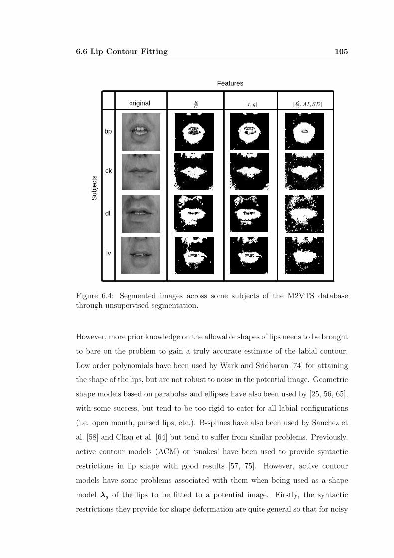
6.6 Lip Contour Fitting 105
ck
original
Features
Sub
ject
s
bp
dl
lvPSfrag replacements
RG
[r, g] [ RG
, AI, SD]
Figure 6.4: Segmented images across some subjects of the M2VTS databasethrough unsupervised segmentation.
However, more prior knowledge on the allowable shapes of lips needs to be brought
to bare on the problem to gain a truly accurate estimate of the labial contour.
Low order polynomials have been used by Wark and Sridharan [74] for attaining
the shape of the lips, but are not robust to noise in the potential image. Geometric
shape models based on parabolas and ellipses have also been used by [25, 56, 65],
with some success, but tend to be too rigid to cater for all labial configurations
(i.e. open mouth, pursed lips, etc.). B-splines have also been used by Sanchez et
al. [58] and Chan et al. [64] but tend to suffer from similar problems. Previously,
active contour models (ACM) or ‘snakes’ have been used to provide syntactic
restrictions in lip shape with good results [57, 75]. However, active contour
models have some problems associated with them when being used as a shape
model λg of the lips to be fitted to a potential image. Firstly, the syntactic
restrictions they provide for shape deformation are quite general so that for noisy
106 6.7 Point Distribution Models and Potential Images
(a) Original Mouth ROI (b) Binary Mouth ROI (c) Potential Image
Figure 6.5: Demonstration of how potential image is created.
potential images the resultant fitted contour may itself be noisy. Secondly, the
potential force fields derived from the potential image, which tell the contour in
which direction to move, have problems associated with the initialisation of the
estimated contour when noise (ie. unwanted visual artifacts or broken lines) is
present.
6.7 Point Distribution Models and Potential Im-
ages
Point distribution models (PDM) have proved to be very good at providing a
model for the deformation of lip contours and in turn provide an accurate way of
locating/tracking a speaker’s lips [24]. PDMs have the advantage of providing a
priori knowledge about typical deformation of lips from a training set of labelled
lips.
The lip contour x can be described by n points
x = (x, y, x, y, ....., xn−, yn−) (6.8)
This contour can be approximated parametrically as λg = (xc,b), where xc
denotes the labial contour’s center and b denotes the labial contour shape found
using principal component analysis (PCA) [24] by,

6.8 Edge Maps and Potential Force Fields 107
x ≈ x + Φb (6.9)
where x is the mean of the training feature vectors, Φ the matrix of the first
few column eigenvectors of the covariance matrix which correspond to the largest
eigenvalues and b a vector containing the weights for each eigenvector. The
vector b can be used as a compact and decorrelated approximate representation
of the original contour vector x in which the main modes of variation have been
preserved.
Point distribution models when used for lip shape location/tracking have been
predominantly implemented within a multidimensional energy minimisation frame-
work [24] that actually differs from the original approach given by Cootes et
al. [59]. Cootes suggested that potential images could be used to calculate sug-
gested movement for each model point such as those used with active contour
models [76]. Adjustments to the position of each point can then be derived from
the potential force field generated from the potential image. Convergence can be
achieved in fewer iterations with the model constrained to vary within valid lip
shapes as dictated by the PDM.
6.8 Edge Maps and Potential Force Fields
As previously mentioned the potential image f(x, y) is a binary edge map derived
from the colour imageRGB(x, y). A potential force field v(x, y) = (u(x, y), v(x, y))
is used to indicate in which direction one must travel to be positioned at the ob-
ject’s edge, where u(x, y) is the x-component and v(x, y) the y-component of
the field respectively. This potential force field is extremely useful for the shape
model fitting process as it gives a method for updating the shape model λg, based
on the rational that as many points as possible in the shape model should be as
108 6.8 Edge Maps and Potential Force Fields
close as possible to an edge. The potential force field v(x, y) is static [77], that
is it does not change as the shape model λg moves or deforms. This is a highly
desirable characteristic as the static nature of the force field ensures a linear,
quickly converging result. Deformable template approaches such as active shape
models [24, 59] and active appearance models [20, 60] can be interpreted as hav-
ing a dynamic force field which changes as the shape model changes, with the
resultant solution being highly non-linear and whose convergence is not assured.
The simplest way to form a force field from a potential image is the gradient of
the potential image v(x, y) = ∇f(x, y) [77]. However, this simplistic field has a
number of problems. Even though the ∇f(x, y) has vectors pointing towards the
edges, the magnitudes are only in the immediate vicinity of the edges. Secondly,
in homogenous regions of f(x, y), ∇f(x, y) is nearly zero. These two problems
make the fitting of a shape model problematic as the capture range around the
edge will be very small, making the whole shape model fitting procedure very
sensitive to how the shape model is initialised. A more robust potential force
field would extend the gradient map farther away from the edges and into ho-
mogenous regions. An additional problem arises due to ∇f(x, y) having vectors
which are normal to the edges at the edges. When a boundary concavity is en-
countered, ∇f(x, y) will have forces pointing in opposite directions within the
concavity. This has the unwanted effect of pointing a shape model to the surface
of the concavity, but not within the concavity [77].
In the next section a new class of potential forces is presented, based on gradient
vector flow (GVF) fields [77], that can evade some of the problems caused by
noisy potential images and traditional potential force fields. Gradient vector flow
(GVF) fields [77] are both insensitive to initialisation and have an ability to move
into concave boundary regions. These fields are used in conjunction with point
distribution models (PDMs) which provide a way to vary a contour based on pre-
trained syntactic information about allowable labial contour deformations. Using
both GVF fields and PDMs a technique has been developed that can reliably

6.9 Gradient Vector Flow 109
converge to the correct lip contour outline whilst maintaining a valid lip shape
under adverse conditions.
6.9 Gradient Vector Flow
The generation of a suitable potential force field v (x, y) from a potential im-
age f(x, y) can be error-prone. First, the initial contour must, in general, be
close to the boundary or else it is likely to converge to a wrong result. Second,
most potential force fields have problems progressing into boundary concavities
which can sometimes restrict a contour from being fitted accurately to a potential
image.
Recently, a new class of potential forces has been proposed that overcomes these
problems. These fields, called gradient vector flow (GVF) fields, are dense vector
fields derived from images by minimizing a certain energy functional in variational
framework [77]. When used with active contour models they have been shown
to be insensitive to initialization and have an ability to move into boundary con-
cavities. A gradient vector flow field can be defined as v(x, y) = (u(x, y), v(x, y))
that minimises the energy functional
E =
∫ ∫
µ(u2x + u2
y + v2x + v2
y) + |∇f |2|v−∇f |dxdy (6.10)
Where µ is a regularization parameter governing the tradeoff between the first
term and the second term in the integrand. This produces the desired effect of
keeping v nearly equal to the gradient of the edge map when it is large, but forcing
the field to be slowly-varying in homogenous regions as can be demonstrated in
Figure 6.6.
To make the process of fitting a contour via the potential force field v as linear
as possible it is convenient to normalise the magnitude of the fields such that the
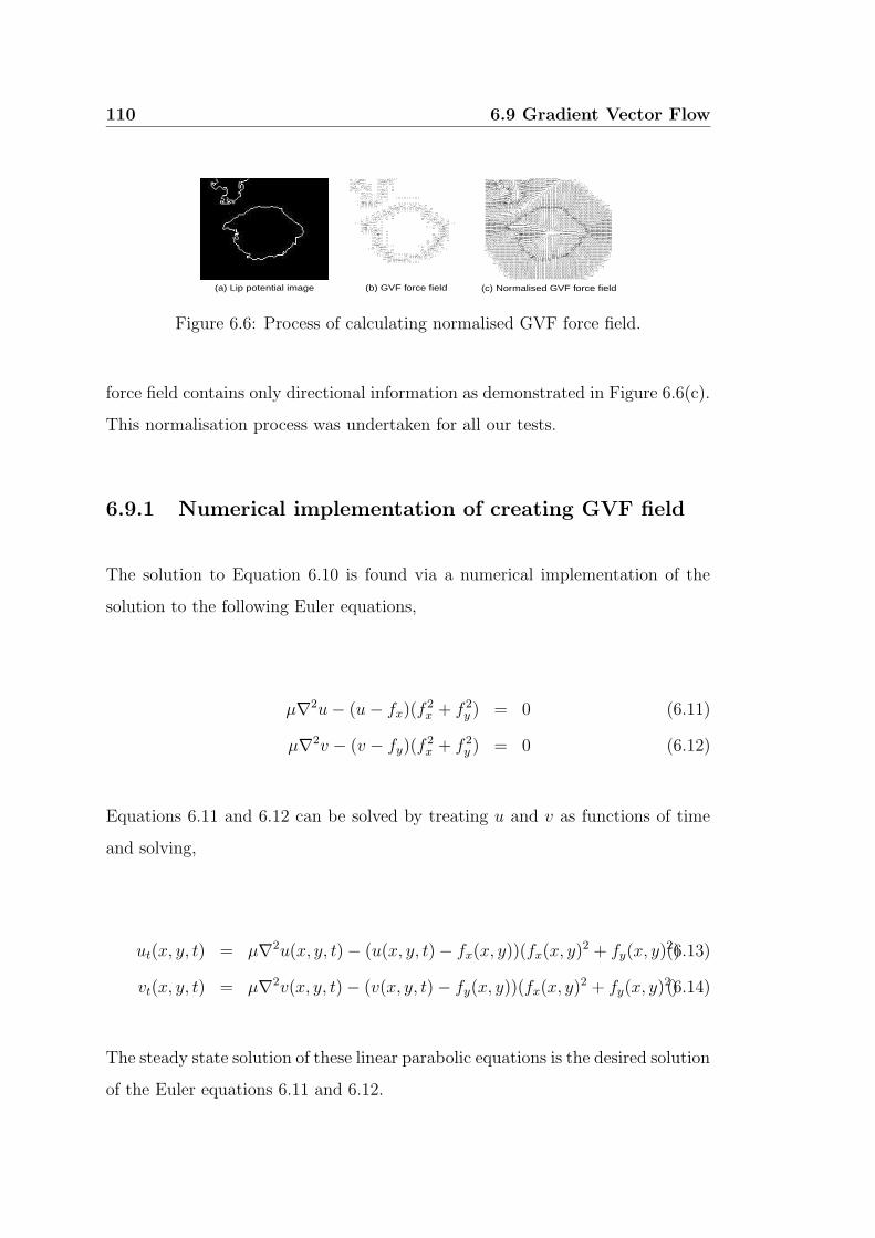
110 6.9 Gradient Vector Flow
(a) Lip potential image (b) GVF force field (c) Normalised GVF force field
Figure 6.6: Process of calculating normalised GVF force field.
force field contains only directional information as demonstrated in Figure 6.6(c).
This normalisation process was undertaken for all our tests.
6.9.1 Numerical implementation of creating GVF field
The solution to Equation 6.10 is found via a numerical implementation of the
solution to the following Euler equations,
µ∇2u− (u− fx)(f2x + f 2
y ) = 0 (6.11)
µ∇2v − (v − fy)(f2x + f 2
y ) = 0 (6.12)
Equations 6.11 and 6.12 can be solved by treating u and v as functions of time
and solving,
ut(x, y, t) = µ∇2u(x, y, t) − (u(x, y, t) − fx(x, y))(fx(x, y)2 + fy(x, y)
2)(6.13)
vt(x, y, t) = µ∇2v(x, y, t) − (v(x, y, t) − fy(x, y))(fx(x, y)2 + fy(x, y)
2)(6.14)
The steady state solution of these linear parabolic equations is the desired solution
of the Euler equations 6.11 and 6.12.

6.10 Calculating Movement for each Model Point 111
6.10 Calculating Movement for each Model Point
The method used for calculating adjustments to shape parameters λg = (xc,b)
based on the GVF field and PDM are very similar to the technique used by
Cootes in [59]. Given an initial estimate of the positions of a set of model points
which one is attempting to fit to a mouth image, and the GVF potential force
field v(x) which points to the proposed outer labial contour, one needs to estimate
a set of adjustments which will move each point toward a better position while
maintaining a valid lip shape. These adjustments can be calculated for each
model point and can be denoted as
dx= (dx, dy, dx, dy, ....., dxn−, dyn−) (6.15)
Where n denotes the number of points representing the contour. Before deforming
the PDM itself one has to first find the approximate center of the lips (xc, yc),
xc= (xc, yc) (6.16)
The need for calculating xc is due to the PDM of the lips being trained in such a
way that the center of the labial contour is at the origin. This was done to ensure
the PDM modelled only the allowable lip shape variation and not translational
variation. As an initial estimate of the lip shape the mean lip shape x of the PDM
was used as per Equation 6.9 with center xc being the position at the center of
the image.
The approach for finding the approximate center of the labial contour is as
follows:-
1. Calculate adjustment vector dx from the
GVF force field v(x+ xc);
112 6.10 Calculating Movement for each Model Point
2. Calculate center adjustment vector
dxc= (dxc, dyc)
where dxc = 1n
∑ni=0 dxi and dyc = 1
n
∑ni=0 dyi;
3. Update xc by new center adjustment vector such that x(t+1)c = x
(t)c + sdxc
where s is step size;
4. Repeat steps 1-3 for n iterations;
In testing a a step size s of one pixel was chosen with the above steps iterated 20
times to be assured of convergence. Once the initial shape estimate is positioned
correctly one can then make adjustments to each model point within the PDM
framework so as to give an optimal fit to the potential image.
The aim is to adjust the shape parameters so as to move the points from their
current locations x and be as close to x+dx as can be arranged whilst still sat-
isfying the shape constraints of the PDM. In [59] it was shown that the optimal
way to calculate adjustments to the shape parameters db of an PDM described
by the weights b in a least squares sense is
db = Φ′dx (6.17)
Using the result obtained in Equation 6.17 one can deform the PDM contour via
the following steps
1. Calculate adjustment vector dx from the
GVF force field v(x+ xc);
2. Calculate db as per Equation 6.17;
3. Update b(t+1) = b(t) + sdb;
4. Get new estimate of x ≈ x + Pb;
6.11 Performance of Lip Location Algorithm 113
5. Repeat steps 1-4 for n iterations;
Again in testing a step size s of one pixel was chosen with the above steps iterated
40 times to be assured of convergence.
6.11 Performance of Lip Location Algorithm
The fusion of PDM based contour deformation and an GVF field gives excellent
tracking performance in a number of trying conditions. This is particularly true
when the labial contour outline in the potential image is obstructed by noise.
Typically there are two types of noise present in segmented mouth ROI images
that cannot be treated effectively through conventional means:-
1. Binary image of lips with unwanted artifacts attached to the binary lip
cluster as seen in Figure 6.7(a).
2. Binary image of lips with missing lip pixels in the binary lip cluster as seen
in Figure 6.8(a).
Using an GVF force field in conjunction with an PDM of the lips, a contour model
can be fitted that gives an excellent estimation of the labial contour circumvent-
ing the noisy artifact present in the potential images shown in Figures 6.7(a)
and 6.8(a). The final results of which can be seen in Figures 6.7(d) and 6.8(d).
The lip location algorithm was run over shots 2 and 3 of the pre-labelled M2VTS
database, so as to get a direct measure of comparison against appearance based
mouth location. Unsupervised segmentation was performed to generate the po-
tential image f(x, y) for each subject. Using the mouth location measure in
Section 4.3.1 (i.e. emouth < 0.25) the entire tracking process obtained a correct
mouth location rate of 82.3%. This rate however, does not reflect the subject
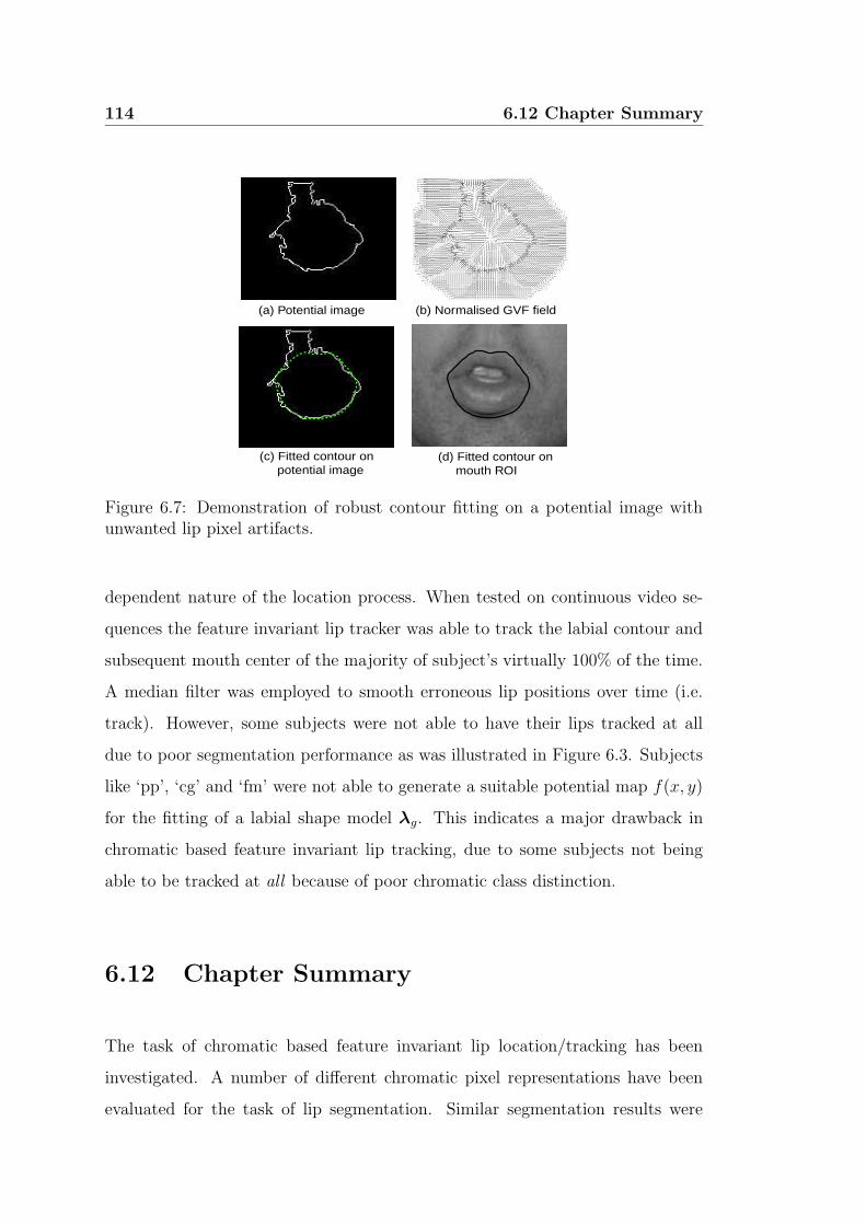
114 6.12 Chapter Summary
(a) Potential image (b) Normalised GVF field
(c) Fitted contour on potential image
(d) Fitted contour on mouth ROI
Figure 6.7: Demonstration of robust contour fitting on a potential image withunwanted lip pixel artifacts.
dependent nature of the location process. When tested on continuous video se-
quences the feature invariant lip tracker was able to track the labial contour and
subsequent mouth center of the majority of subject’s virtually 100% of the time.
A median filter was employed to smooth erroneous lip positions over time (i.e.
track). However, some subjects were not able to have their lips tracked at all
due to poor segmentation performance as was illustrated in Figure 6.3. Subjects
like ‘pp’, ‘cg’ and ‘fm’ were not able to generate a suitable potential map f(x, y)
for the fitting of a labial shape model λg. This indicates a major drawback in
chromatic based feature invariant lip tracking, due to some subjects not being
able to be tracked at all because of poor chromatic class distinction.
6.12 Chapter Summary
The task of chromatic based feature invariant lip location/tracking has been
investigated. A number of different chromatic pixel representations have been
evaluated for the task of lip segmentation. Similar segmentation results were
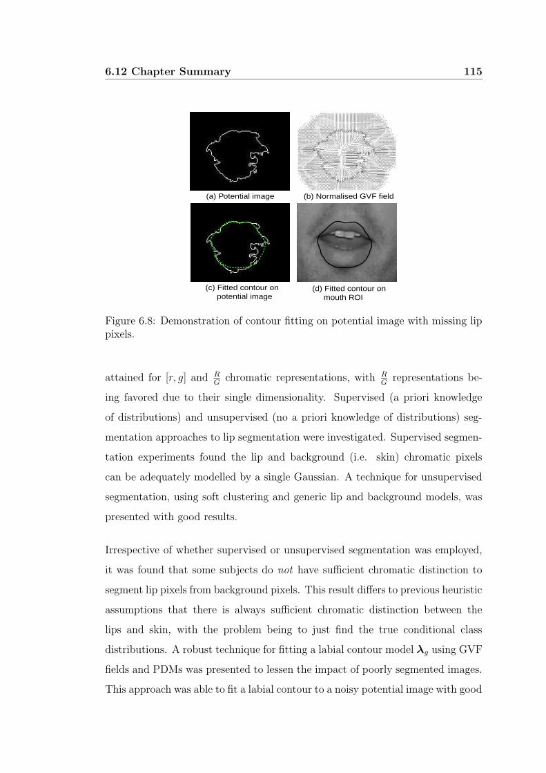
6.12 Chapter Summary 115
(b) Normalised GVF field(a) Potential image
(c) Fitted contour on potential image
(d) Fitted contour on mouth ROI
Figure 6.8: Demonstration of contour fitting on potential image with missing lippixels.
attained for [r, g] and RG
chromatic representations, with RG
representations be-
ing favored due to their single dimensionality. Supervised (a priori knowledge
of distributions) and unsupervised (no a priori knowledge of distributions) seg-
mentation approaches to lip segmentation were investigated. Supervised segmen-
tation experiments found the lip and background (i.e. skin) chromatic pixels
can be adequately modelled by a single Gaussian. A technique for unsupervised
segmentation, using soft clustering and generic lip and background models, was
presented with good results.
Irrespective of whether supervised or unsupervised segmentation was employed,
it was found that some subjects do not have sufficient chromatic distinction to
segment lip pixels from background pixels. This result differs to previous heuristic
assumptions that there is always sufficient chromatic distinction between the
lips and skin, with the problem being to just find the true conditional class
distributions. A robust technique for fitting a labial contour model λg using GVF
fields and PDMs was presented to lessen the impact of poorly segmented images.
This approach was able to fit a labial contour to a noisy potential image with good

116 6.12 Chapter Summary
results. Unfortunately, for some subjects the potential images were too noisy, due
to poor segmentation, for adequate mouth location/tracking. Feature invariant
lip tracking, although useful, was deemed to susceptible to subject variation for
effective use in an AVSP application and is not used in the rest of this thesis.
Chapter 7
Feature Extraction
7.1 Introduction
In pattern recognition [35, 37], from a theoretical perspective, the distinction
between feature extraction and classification is blurred. An ideal feature extractor
would yield measurements that make the job of a classifier trivial. Similarly, an
ideal classifier would not require the help of a sophisticated feature extractor.
The distinction between feature extraction and classification manifests itself for
practical rather than theoretical reasons.
Feature extraction seeks to find representations of an observation that provide dis-
crimination between objects of different categories whilst providing invariance to
irrelevant transforms on observations who are in the same class. Ideally, if one
had an infinite amount of training observations describing all classes wanting to
be discriminated between; one could gain a model p(o|ωi) of all possible manifes-
tations of observation o in a class ωi removing the need for feature extraction.
This approach is infeasible on two accounts. Firstly, due to practical constraints
one may never obtain an infinite amount of training observations. Secondly, and
most importantly, the domain in which the observation o is represented may
118 7.2 Acoustic Speech Features
not provide sufficient class distinction between classes or invariance to irrelevant
transformations. The task of feature extraction is to find a domain for repre-
senting an observation o that contains suitable class distinction and irrelevant
transform invariance whilst being of a compact enough form to train a classifier
from a finite number of observations.
AVSP requires the extraction and analysis of both acoustic and visual features for
processing. Acoustic analysis has been well studied for many decades [6, 8, 78].
Researchers have developed a number of ways to parameterize speech waveforms.
For example, the use of filter bank outputs and cepstral coefficients [45, 48, 79]
has proven very effective for speech and speaker recognition. The question arises
of how to effectively represent the visual signal (ie. mouth shape, area and move-
ment). The answer to this question is still unclear and is the subject of consider-
able research.
7.2 Acoustic Speech Features
Acoustic speech processing is a more mature field in comparison to its visual coun-
terpart. Considerable insight, over the past couple of decades, has been gained
into what features perform best for specific audio speech applications (i.e. speech
recognition, enhancement, coding and speaker identification/verification) [45, 79].
Acoustic speech is a naturally varying continuous signal whose statistics change
with time. A problem results into how to break it up into observation feature
vectors suitable for processing. Fortunately, speech varies slow enough to as-
sume its statistics are quasi-stationary over segments up to 100 milliseconds in
duration [80].
To circumvent problems with windowing, particularly discontinuities arising from
Gibb’s phenomenon [81], a hamming window is employed to segment the speech
signal. For speech and speaker recognition applications a window size of 25ms
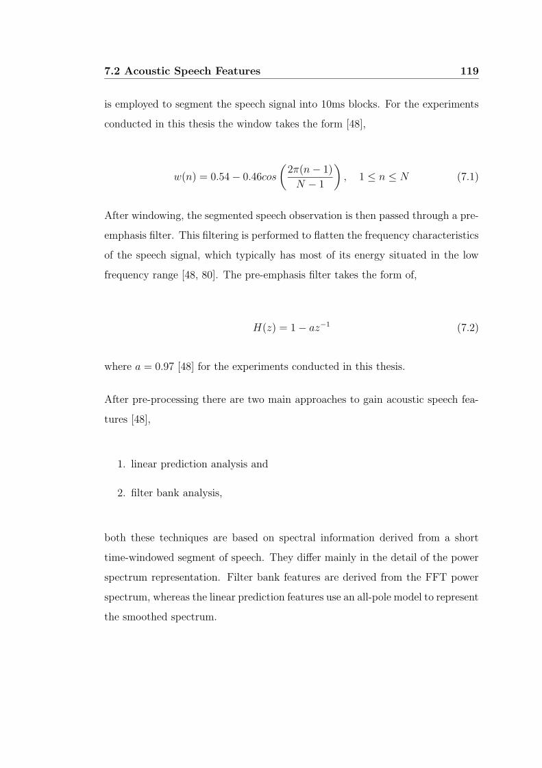
7.2 Acoustic Speech Features 119
is employed to segment the speech signal into 10ms blocks. For the experiments
conducted in this thesis the window takes the form [48],
w(n) = 0.54 − 0.46cos
(2π(n− 1)
N − 1
)
, 1 ≤ n ≤ N (7.1)
After windowing, the segmented speech observation is then passed through a pre-
emphasis filter. This filtering is performed to flatten the frequency characteristics
of the speech signal, which typically has most of its energy situated in the low
frequency range [48, 80]. The pre-emphasis filter takes the form of,
H(z) = 1 − az−1 (7.2)
where a = 0.97 [48] for the experiments conducted in this thesis.
After pre-processing there are two main approaches to gain acoustic speech fea-
tures [48],
1. linear prediction analysis and
2. filter bank analysis,
both these techniques are based on spectral information derived from a short
time-windowed segment of speech. They differ mainly in the detail of the power
spectrum representation. Filter bank features are derived from the FFT power
spectrum, whereas the linear prediction features use an all-pole model to represent
the smoothed spectrum.
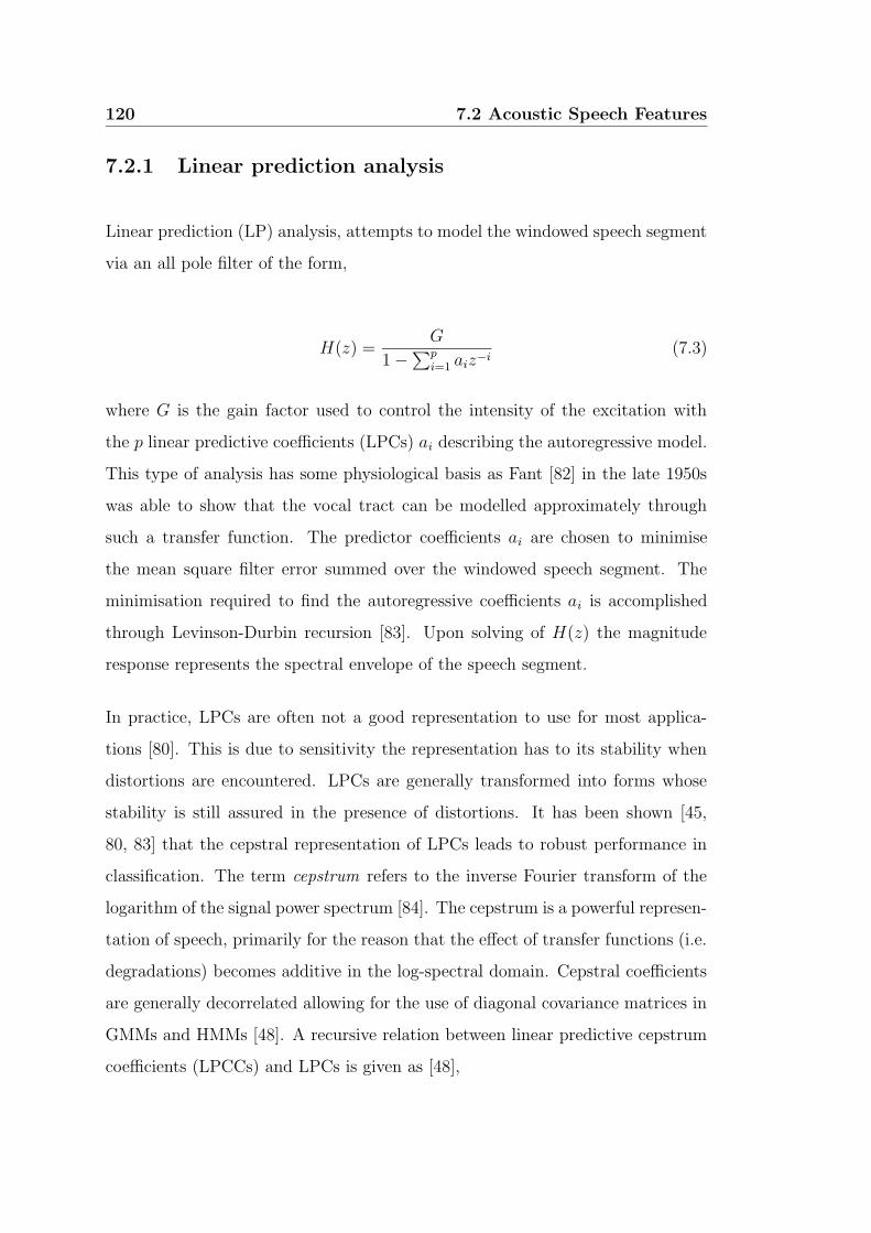
120 7.2 Acoustic Speech Features
7.2.1 Linear prediction analysis
Linear prediction (LP) analysis, attempts to model the windowed speech segment
via an all pole filter of the form,
H(z) =G
1 −∑p
i=1 aiz−i(7.3)
where G is the gain factor used to control the intensity of the excitation with
the p linear predictive coefficients (LPCs) ai describing the autoregressive model.
This type of analysis has some physiological basis as Fant [82] in the late 1950s
was able to show that the vocal tract can be modelled approximately through
such a transfer function. The predictor coefficients ai are chosen to minimise
the mean square filter error summed over the windowed speech segment. The
minimisation required to find the autoregressive coefficients ai is accomplished
through Levinson-Durbin recursion [83]. Upon solving of H(z) the magnitude
response represents the spectral envelope of the speech segment.
In practice, LPCs are often not a good representation to use for most applica-
tions [80]. This is due to sensitivity the representation has to its stability when
distortions are encountered. LPCs are generally transformed into forms whose
stability is still assured in the presence of distortions. It has been shown [45,
80, 83] that the cepstral representation of LPCs leads to robust performance in
classification. The term cepstrum refers to the inverse Fourier transform of the
logarithm of the signal power spectrum [84]. The cepstrum is a powerful represen-
tation of speech, primarily for the reason that the effect of transfer functions (i.e.
degradations) becomes additive in the log-spectral domain. Cepstral coefficients
are generally decorrelated allowing for the use of diagonal covariance matrices in
GMMs and HMMs [48]. A recursive relation between linear predictive cepstrum
coefficients (LPCCs) and LPCs is given as [48],
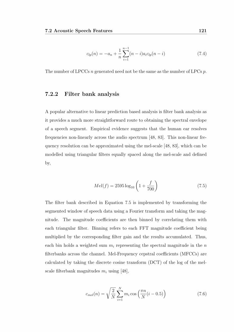
7.2 Acoustic Speech Features 121
clp(n) = −an +1
n
n−1∑
i=1
(n− i)aiclp(n− i) (7.4)
The number of LPCCs n generated need not be the same as the number of LPCs p.
7.2.2 Filter bank analysis
A popular alternative to linear prediction based analysis is filter bank analysis as
it provides a much more straightforward route to obtaining the spectral envelope
of a speech segment. Empirical evidence suggests that the human ear resolves
frequencies non-linearly across the audio spectrum [48, 83]. This non-linear fre-
quency resolution can be approximated using the mel-scale [48, 83], which can be
modelled using triangular filters equally spaced along the mel-scale and defined
by,
Mel(f) = 2595 log10
(
1 +f
700
)
(7.5)
The filter bank described in Equation 7.5 is implemented by transforming the
segmented window of speech data using a Fourier transform and taking the mag-
nitude. The magnitude coefficients are then binned by correlating them with
each triangular filter. Binning refers to each FFT magnitude coefficient being
multiplied by the corresponding filter gain and the results accumulated. Thus,
each bin holds a weighted sum mi representing the spectral magnitude in the n
filterbanks across the channel. Mel-Frequency cepstral coefficients (MFCCs) are
calculated by taking the discrete cosine transform (DCT) of the log of the mel-
scale filterbank magnitudes mi using [48],
cmel(n) =
√
2
N
N∑
i=1
mi cos(πn
N(i− 0.5)
)
(7.6)

122 7.2 Acoustic Speech Features
where N is the number of filterbank channels. Filterbank amplitudes mi are
highly correlated, the use of an DCT transform is employed to try and remove
some of this correlation. A cepstral representation was used due to its robust be-
havior in the presence of various sources of degradation. In all experiments in this
thesis MFCCs were used as our acoustic features through the HTK package [48].
Although much work is still to be done [85] in the field of acoustic feature extrac-
tion for speech processing standard techniques shall be drawn on for the duration
of this thesis. It has been shown in previous work that filter bank based MFCCs
perform extremely well for the tasks of speech recognition [79] and speaker recog-
nition [45] in comparison to linear prediction based representations.
7.2.3 Improving robustness to acoustic train/test
mismatches
As will become apparent through much of this thesis, train/test mismatches can
drastically affect the performance of a classifier whether it be in the acoustic
of visual modality. If one can provide some sort of invariance to a train/test
mismatch in the feature representation of an input signal, then the entire system
will reap the benefits of the invariance. Commonly train/test mismatches can in
the acoustic speech domain be attributed to changes in the channel conditions
and noise [83]. A number of approaches have been devised to lessen the effects
of these type of train/test mismatches.
Cepstral weighting
Cepstral weighting attempts to compensate for the sensitivity of the low-order
cepstral coefficients to overall spectral slope and the sensitivity of the high-order
cepstral coefficients to noise [84]. Liftering is usually the name given to this type
of weighting. This is performed for all experiments conducted in this thesis by
applying the following formula to the cepstrum [48],
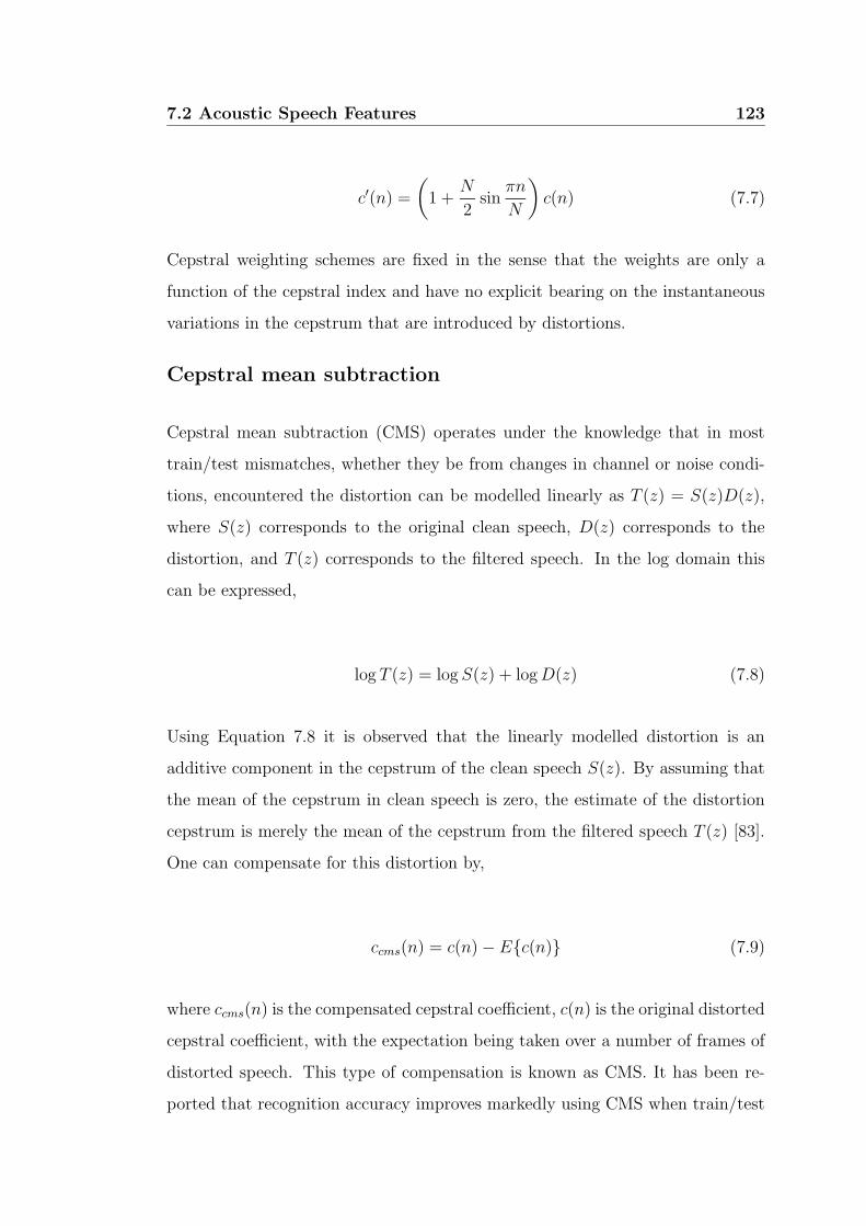
7.2 Acoustic Speech Features 123
c′(n) =
(
1 +N
2sin
πn
N
)
c(n) (7.7)
Cepstral weighting schemes are fixed in the sense that the weights are only a
function of the cepstral index and have no explicit bearing on the instantaneous
variations in the cepstrum that are introduced by distortions.
Cepstral mean subtraction
Cepstral mean subtraction (CMS) operates under the knowledge that in most
train/test mismatches, whether they be from changes in channel or noise condi-
tions, encountered the distortion can be modelled linearly as T (z) = S(z)D(z),
where S(z) corresponds to the original clean speech, D(z) corresponds to the
distortion, and T (z) corresponds to the filtered speech. In the log domain this
can be expressed,
log T (z) = log S(z) + logD(z) (7.8)
Using Equation 7.8 it is observed that the linearly modelled distortion is an
additive component in the cepstrum of the clean speech S(z). By assuming that
the mean of the cepstrum in clean speech is zero, the estimate of the distortion
cepstrum is merely the mean of the cepstrum from the filtered speech T (z) [83].
One can compensate for this distortion by,
ccms(n) = c(n) − Ec(n) (7.9)
where ccms(n) is the compensated cepstral coefficient, c(n) is the original distorted
cepstral coefficient, with the expectation being taken over a number of frames of
distorted speech. This type of compensation is known as CMS. It has been re-
ported that recognition accuracy improves markedly using CMS when train/test
124 7.3 Visual Speech Features
mismatches are encountered [48, 83]. However, some loss in recognition accuracy
is experienced when CMS is employed when there is no train/test mismatch.
This is due to the implicit assumption in CMS that the long-term cepstral mean
is zero, an assumption that may not always hold [83]. CMS is particularly useful
in improving recognition performance in the presence of acoustic train/test mis-
matches and is used in all acoustic cepstral speech experiments conducted in this
thesis unless otherwise specified.
Other robust cepstral techniques
The relative spectral (RASTA) technique [86] takes advantage of the fact that the
rate of change of nonlinguistic components in speech often lies outside the typical
rate of change of the vocal-tract shape. Therefore, it suppresses the spectral
components that change more slowly or quickly than the typical rate of change
of speech. The use of RASTA processing has been shown to improve speech
recognition performance in the presence of mismatches [86].
7.3 Visual Speech Features
It is largely agreed upon that the majority of visual speech information stems
from a subject’s mouth [12]. The field of AVSP is still in a state of relative
infancy, during the period of its short existence a majority of the work performed
has been towards the goal of finding the best mouth representation for the tasks
of audio-visual speech and speaker recognition. Usually, these representations are
based on the techniques used to initially locate and track the mouth, as described
in-depth in Chapter 4, due to their ability to parametrically describe the mouth
in a compact enough form for use in statistical classification.
The mouth can be represented in several domains, however they can be cate-
gorised broadly into two representations for AVSP which are [30, 57],
7.3 Visual Speech Features 125
1. area representations, and
2. contour representations.
Area based representations are concerned with transforming the whole input
mouth intensity image into a meaningful feature vector. Contour based rep-
resentations are concerned with parametrically atomizing the mouth, based on
a priori knowledge of the components of the mouth (i.e. outer and inner labial
contour, tongue, teeth, etc.). For both representations it is assumed that the
mouth has been located and suitably normalised for face scale.
7.3.1 Area based representations
The most common technique used to gain a holistic compact representation of
a mouth is through the use of principal component analysis (PCA), described
previously in Section 5.1.2, on the mouth ROI intensity image. Bregler and
Konig [87] in his eigenlips technique was one of the first to apply PCA as an
compact area representation of the mouth; PCA has been used as a visual feature
for audio visual speech recognition in separate subsequent research [57, 88, 89].
PCA is a useful tool for gaining a compact representation of the mouth, but uses
the suboptimal criterion of reconstruction error as its criterion for generating a
subspace.
Linear discriminant analysis (LDA), as previously described in Section 5.1.3,
generates a subspace based on a measure of class discrimination. LDA rep-
resentations have become extremely useful in AV speech [24, 28, 90, 91] and
speaker [26, 27] recognition applications. Potamianos et al. [28] was able to im-
prove audio-visual speech recognition performance further through the use of a
maximum likelihood linear transform (MLLT) which maximises the observations
in the LDA feature space, under the assumption of a diagonal covariance. This
type of transform is of benefit due to classifiers in most speech applications (i.e.
126 7.3 Visual Speech Features
GMMs and HMMs) using diagonal covariance matrices. Independent compo-
nent analysis (ICA) has also been used as a form of visual feature extraction
for automated speech reading [89]. The goal of ICA [92] is to perform nonlinear
monotonic transformations such that the transformed representation is statisti-
cally independent, not just uncorrelated. However, results received using such a
transform were not significantly better than traditional PCA representations [89]
for the task of speech reading. All feature extraction approaches mentioned thus
far are data driven, that is they require training observations of mouth ROI im-
ages to create their compact representation of the mouth. Data driven approaches
can have drawbacks in that they are very sensitive to the training observation
ensemble used to create the mouth subspace.
Non-data driven transforms have been previously used such as the discrete wavelet
transform (DWT) [30, 93] and the discrete cosine transform (DCT) [25, 28] di-
rectly or as pre-processing stage for visual feature extraction. Both DCT and
DWT mouth representations generally require higher dimensional feature vectors
than PCA to reach optimal performance, which is a serious consideration when
the number of training observations are finite. A paper by Matthews et al. [20]
used a non-linear transform called multiscale spatial analysis (MSA) to gain a
representation of the mouth. MSA uses a nonlinear scale-space decomposition
algorithm called a sieve which is a mathematical morphology serial filter struc-
ture that progressively removes features from an image by increasing the scale.
These non-data driven approaches have the benefit of not being dependent on a
training ensemble, but bring minimal a priori knowledge about the mouth to the
problem of visual speech and speaker recognition.
There has been some argument put forward by Gray et al. [89] for a localised
representation of the mouth, as opposed to the non-local approaches previously
mentioned (i.e. each image in the basis set has non-zero energy distributed about
the whole image). In this approach localised kernels are convolved across an 2-D
mouth image to try and extract spatially localised visual speech information from
7.3 Visual Speech Features 127
the mouth. A variety of kernels were employed based on data driven techniques
such as PCA (eigenpatches) and ICA, as well as simple Gaussian kernels. Al-
though showing some promise, the dimensionality of the localised representation
was too great to be of any real use in a suitably trained and complex statistical
classifier (eg. HMM).
7.3.2 Contour based representations
For contour based techniques, one has the same problem in locating components
of the mouth as in Chapter 4 and 6, as they are the manifestation of the same
problem simply used for a different purpose. Contour information describing the
mouth is usually associated with finding the outer labial contour of the mouth.
Other approaches have attempted to extract the inner labial contour, tongue
and teeth [4, 66, 94], but have received mixed results due to the difficulty and
lack of class distinction associated with the task. Previous work [95, 96] has
coloured a speaker’s lips with blue ink prior to labial contour location. Due to
the colouring, the outer and inner labial contour can easily be located. However,
such an approach is not useful in practical applications.
Techniques for locating and fitting the outer labial contour of a speaker have pre-
viously been discussed in Chapter 6. With reference to visual feature extraction,
contour representations are concerned with how best to describe the labial con-
tour to get maximum classification performance in an AVSP application. Chiou
and Hwang [57] used distances taken radially around the center of the lip con-
tour with good results. Chen et al. [6, 25] used lip width and the upper and
lower lip height as a visual feature. Sanchez et al. [58] and Chan et al. [64] both
used parametric representation of the B-spline describing the labial contour as
a visual feature. Although useful, these representations do not give much detail
about the labial contour. Techniques that employed point distribution models
(PDMs) [18, 20, 66, 97] received good performance as this approach used the
128 7.3 Visual Speech Features
weights describing the contour within a restricted eigen-contour space. The tech-
nique was able to convey far more detail about the labial outline than previous
approaches. Gurbuz et al. [98] employed an affine-invariant fourier descriptors
to describe the outer labial contour. This representation was able to provide
invariance to affine invariant transforms on the contour, which reportedly gave
an increase in robustness. All techniques are however, totally dependent on their
ability to first locate the outer labial contour.
7.3.3 Area vs. contour features
Area representations have a certain appeal over contour representations of the
mouth. It has been reported by Chiou et al. [57] that the variation of the gray
levels around human lips is small, making the atomization of the mouth into
basic components a difficult task. Chapter 6 demonstrated that colour can be
used to improve this distinction, however this assumption does not always hold as
some subjects report very poor chromatic class distinction between the lips and
skin. The mouth at the best of times does not have strict boundaries of demar-
cation between its respective components (eg. inner and outer labial contours,
tongue, teeth). Area features do not suffer from such problems as all information
pertaining to the mouth is contained holistically within the mouth ROI image
representation.
Contour representations of the mouth have certain benefits over area based rep-
resentations. The main benefit can be found in the invariance provided from
contour representations. Area features tend to suffer from irrelevant variations
pertaining to visual speech. Variances due to lighting and subject appearance
(identity for speech and pronunciation for speaker recognition) can radically af-
fect classification performance. The accuracy of physically extracting the outer
labial contour of some subjects is difficult, with convergence to a satisfactory lip
shape not always assured. Area features rely on simple transforms based on the
7.3 Visual Speech Features 129
mouth ROI image making them far more stable in robust conditions over their
contour counterparts.
There has been some research performed by [18, 20, 57, 66] indicating there is
some benefit in using a joint area and contour based representation. This type
of approach works under the premise that there is benefit in fusing the invariant
properties of contour representations with the holistic properties of area repre-
sentations. In this approach the contour and area representation is concatenated
into a single feature vector. These approaches, although useful, are again totally
dependent on their ability to first locate the outer labial contour. Additionally,
work by [30] has shown that in some cases the combination of contour and area
features can degrade visual speech recognition performance.
In a recent paper by Potamianos et al. [30] a review was conducted between
area and contour features for the tasks of speechreading on a large audio visual
database. In this paper it was shown that area representations obtained superior
performance. Area based representations of the mouth were shown to be robust
to noise and compression artifacts and are the mouth representation of choice in
current AVSP work. Recent work at IBM [24, 28, 91] has seen the completion of
the most comprehensive continuous audio-visual speech recognition experiments
conducted to date. In this work, experiments were carried out over 290 subjects
with over 2.5 hours of speech, in all experiments area features were employed
enjoying good and stable results. Within this thesis, due to the need for robust
and stable visual features in AVSP, and due to the holistic nature of the repre-
sentation, area features were used for all AVSP experiments conducted for the
tasks of speech and speaker recognition.
130 7.4 Delta Features
7.4 Delta Features
An important aspect of feature selection is taking into account the structure,
assumptions and limitations of the classifier being used to make the final decision.
As mentioned in Chapter 3, the classifier of choice for speech recognition, and text
dependent speaker recognition is the hidden Markov model (HMM). HMMs are
extremely useful for speech processing as they can naturally model the temporal
fluctuations of speech in a manner that is invariant to the actual length of the
utterance. However, HMMs do have some inherent limitations which are in direct
conflict to the true nature of speech. The assumptions specifically affecting speech
and speaker recognition are [37, 99, 100],
Piece-wise stationarity: assumes that speech is produced by piece-wise sta-
tionary process with instantaneous transitions between stationary states.
Independence assumption: probability of a speech feature given a model state
depends only on the speech feature vector and the state. No dependency
of observations, other than through the state sequence, is assumed.
Speech production is not a piece-wise stationary process, but a continuous one,
where changes are mostly smoothly time varying. Constraints of articulation
are such that any one frame of speech is highly correlated with previous and
following frames. The performance of HMM based speech and text dependent
speaker recognition systems can be greatly enhanced by adding time derivatives
to the basic static features [48]. Initial work by Bregler and Konig [87] noted
the importance of delta features in visual speech recognition, as they were able
to improve recognition performance in all cases. Delta features are computed in
this thesis using the following regression formula [48],
dt =Θ∑
θ=1
θ(ot+θ − ot−θ)
2∑Θ
θ=1 θ2
(7.10)
7.5 Evaluation of Speech Features 131
where ot is a static speech feature at time index t, a value of Θ = 3 received good
performance experimentally in both acoustic and visual speech modalities. The
final speech vector o∆t used in classification is simply the concatenation of the
static and dynamic features such that,
o∆t = ot,dt (7.11)
Since Equation 7.10 relies on past and future speech features, some modifications
are needed at the beginning and end of a speech sequence. In experiments con-
ducted within this thesis the behavior is to replicate the first or last vector as
needed to fill the regression window in Equation 7.10.
7.5 Evaluation of Speech Features
The actual evaluation of visual speech features is not an easy task as an inherent
problem with extracting speech features is in getting an accurate measure of how
well a given speech feature works when compared against another. Luettin [66]
proposed that an accurate measure of the quality of visual features is indicative
of how well it performs in the task it is being used for, which in this case is visual
speech and text dependent speaker recognition. As previously mentioned, only
area features shall be investigated in this thesis due to their robustness and ability
to holistically represent the mouth. Data-driven feature extraction approaches
were investigated solely in this evaluation due to their natural ability to bring a
priori knowledge of the mouth to the representation. The tasks of speech and
speaker recognition were tested with the following visual features,
PCA: in which PCA was used to create a twenty dimensional subspace ΦPCA
preserving the 20 highest linear modes of mouth variation. This feature
extraction approach was employed for both speech and speaker recognition.
132 7.5 Evaluation of Speech Features
SLDA: in which LDA was used to create a twenty dimensional subspace ΦSLDA
for the speaker recognition task using a priori knowledge of the subject
classes to generate the 20 most discriminant basis vectors.
MRPCA: in which the mean removed mouth sub-image y∗ is calculated from
a given temporal mouth sub-image sequence Y = y1, . . . ,yT such that,
y∗t = yt − y (7.12)
where,
y =1
T
T∑
t=1
yt (7.13)
This approach is very similar to cepstral mean substraction [48] used on
acoustic cepstral features to improve recognition performance by provid-
ing some invariance to unwanted variations. In the visual scenario this
unwanted variation usually stems from subject appearance. Mean-removal
PCA (MRPCA) uses these newly adjusted y∗ mouth sub-images to create a
new twenty dimensional subspace ΦMRPCA preserving the 20 highest modes
of mean removed mouth variation. This approach was first proposed by
Potamianos et al. [30] for improved visual speech recognition performance.
WLDA: in which LDA was used to create a nine dimensional subspace ΦWLDA
for the speech recognition task using a priori knowledge of the word classes
to generate the 9 most discriminant basis vectors. Mean removal, similar
to the approach used for MRPCA, was first employed to remove unwanted
subject variances from the WLDA feature extraction process.
A compact representation of the mouth sub-image y can be obtained by the linear
transform,
o = Φ′y (7.14)
7.5 Evaluation of Speech Features 133
such that o is the compactly represented visual speech observation feature vector.
Illumination invariance was obtained by normalising the vectorised mouth inten-
sity sub-image y to a zero-mean unit-norm vector [39]. For the generation of the
LDA subspaces, PCA was first employed to preserve the first 50 linear modes of
variation, in order to remove any low energy noise that may corrupt classification
performance. For all subspaces, shots one to three of the M2VTS database were
used as training mouth observations, with shot four being used for testing in the
speech and speaker recognition tasks.
7.5.1 Training of hidden Markov models
Hidden Markov models (HMMs) were used to model the video utterances using
HTK ver 2.2. [48]. The first three shots of the M2VTS database were used to train
the visual HMMs with shot four being used for testing. The database consisted
of 36 subjects (male and female) speaking four repetitions (shots) of ten French
digits from zero to nine. In the task of speech recognition the word error rate
(WER) was used as a measure of performance for the ten digits being recognised
in the M2VTS database.
Speaker recognition encapsulates two tasks, namely speaker identification and
verification. Speaker error rate (SER) was used to gauge the effectiveness of
visual features for speaker identification. The SER metric was deemed useful
enough for gauging the effectiveness of visual features in speaker recognition as
good performance in the speaker identification task generally translates well for
the verification task. Due to the relatively small size of the M2VTS database and
the requirement for separate speaker dependent digit HMMs, all speaker depen-
dent HMM digit models were trained by initialising training with the previously
found speaker independent or background digit model. This approach prevented
variances in each model becoming too small and allows each model to converge
to sensible values for the task of text dependent speaker recognition.
134 7.5 Evaluation of Speech Features
7.5.2 Speech recognition performance
Table 7.1 shows the WER for the task of digit recognition on the M2VTS database.
Raw PCA features have the worse WER performance out of all the visual fea-
tures evaluated. There is little difference between the MRPCA and WLDA area
representation of the mouth in terms of WER at the normal video sample rate
of 40ms, with WLDA visual features performing slightly better. Acoustic MFCC
features were also evaluated in Table 7.1 for comparison with its visual coun-
terparts. The train and test sets of each feature type were evaluated in terms
of WER. The difference between train and test WERs is very important as this
gives an indication of how undertrained a specific speech recognition classifier is
using a certain type of feature [23]. The train WER is also very important as it
gives a rough estimate of the lower Bayes error for that feature representation,
with the test WER giving an estimate of the upper Bayes error. Both train and
test errors are essential to properly evaluate a feature set.
There are very large differences between train and test WERs for all visual feature
sets in comparison to the differences seen in the acoustic MFCC feature set.
Additionally, the test WERs for all visual features are quite large, which is in
stark contrast to the acoustic MFCCs which received negligible error. This may
indicate the inherent variability of the chosen visual features is higher than those
found in conventional acoustic features, or that the visual features do not provide
enough distinction between word classes using a standard HMM classifier. Similar
results were received by Cox et al. [23] pertaining to the undertrained nature of
standard HMM based visual speech recognition classifiers.
Initially, one may assume the undertrained nature of the visual HMM classifiers
may be attributed to the acoustic modality having four times as many training
observations as the visual modality. This is due to the acoustic speech signal
being sampled at a 10m intervals, with the visual speech signal being sampled at
a coarser 40ms interval. To partially remedy this situation, the visual features
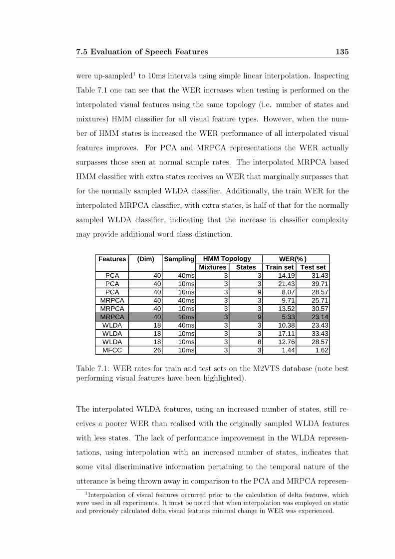
7.5 Evaluation of Speech Features 135
were up-sampled1 to 10ms intervals using simple linear interpolation. Inspecting
Table 7.1 one can see that the WER increases when testing is performed on the
interpolated visual features using the same topology (i.e. number of states and
mixtures) HMM classifier for all visual feature types. However, when the num-
ber of HMM states is increased the WER performance of all interpolated visual
features improves. For PCA and MRPCA representations the WER actually
surpasses those seen at normal sample rates. The interpolated MRPCA based
HMM classifier with extra states receives an WER that marginally surpasses that
for the normally sampled WLDA classifier. Additionally, the train WER for the
interpolated MRPCA classifier, with extra states, is half of that for the normally
sampled WLDA classifier, indicating that the increase in classifier complexity
may provide additional word class distinction.
Features (Dim) Sampling HMM Topology WER(% )Mixtures States Train set Test set
PCA 40 40ms 3 3 14.19 31.43PCA 40 10ms 3 3 21.43 39.71PCA 40 10ms 3 9 8.07 28.57
MRPCA 40 40ms 3 3 9.71 25.71MRPCA 40 10ms 3 3 13.52 30.57MRPCA 40 10ms 3 9 5.33 23.14WLDA 18 40ms 3 3 10.38 23.43WLDA 18 10ms 3 3 17.11 33.43WLDA 18 10ms 3 8 12.76 28.57MFCC 26 10ms 3 3 1.44 1.62
Table 7.1: WER rates for train and test sets on the M2VTS database (note bestperforming visual features have been highlighted).
The interpolated WLDA features, using an increased number of states, still re-
ceives a poorer WER than realised with the originally sampled WLDA features
with less states. The lack of performance improvement in the WLDA represen-
tations, using interpolation with an increased number of states, indicates that
some vital discriminative information pertaining to the temporal nature of the
utterance is being thrown away in comparison to the PCA and MRPCA represen-
1Interpolation of visual features occurred prior to the calculation of delta features, whichwere used in all experiments. It must be noted that when interpolation was employed on staticand previously calculated delta visual features minimal change in WER was experienced.
136 7.5 Evaluation of Speech Features
tations. This could be attributed to the majority of discriminatory information
between words being contained in the temporal nature of the pronunciation not
the static appearance. A major drawback in WLDA feature extraction seems to
stem from its inability to form a discriminative subspace based on the dynamic,
not just static, nature of the signal. Potamianos et al. [101] devised an approach
to circumvent this limitation by incorporating contextual information about adja-
cent frames into the construction of a discriminative subspace. Although showing
some improvement, this approach fails to address some of the fundamental prob-
lems associated with using a standard HMM classifier for speech reading.
The performance improvement from the interpolation of PCA and MRPCA fea-
tures along with the increase in HMM states for their respective HMM classifiers
can be considered to be counter intuitive, as no extra information is being added
to the interpolated visual features apart from the delta features which are de-
pendent on the sample rate of the signal. The benefit of interpolating visual
features can be understood from work done by Deng [99] concerning standard
HMM based speech recognition. Deng has argued that the use of many states
in a standard HMM can approximate continuously varying, non-stationary, pat-
terns in a piecewise constant fashion. Further, it was found in previous acoustic
speech recognition work [100, 102, 103], that as many as ten states are needed to
model strongly dynamic speech segments in order to achieve a reasonable recog-
nition performance. Similar results were found by Matthews et al. [20] for visual
speech recognition where as many as nine states were required, after visual feature
interpolation, to achieve reasonable WERs.
It has been postulated by Deng [99] that employing extra states in a standard
HMM to better model the non-stationary dynamic nature of a signal in a piece-
wise manner has obvious shortcomings. This is due to the many free and largely
independent parameters needing to be found by the addition of extra states which
requires a large amount of training observations for reliable classification. The
problems concerning the lack of training observations can be partially combated
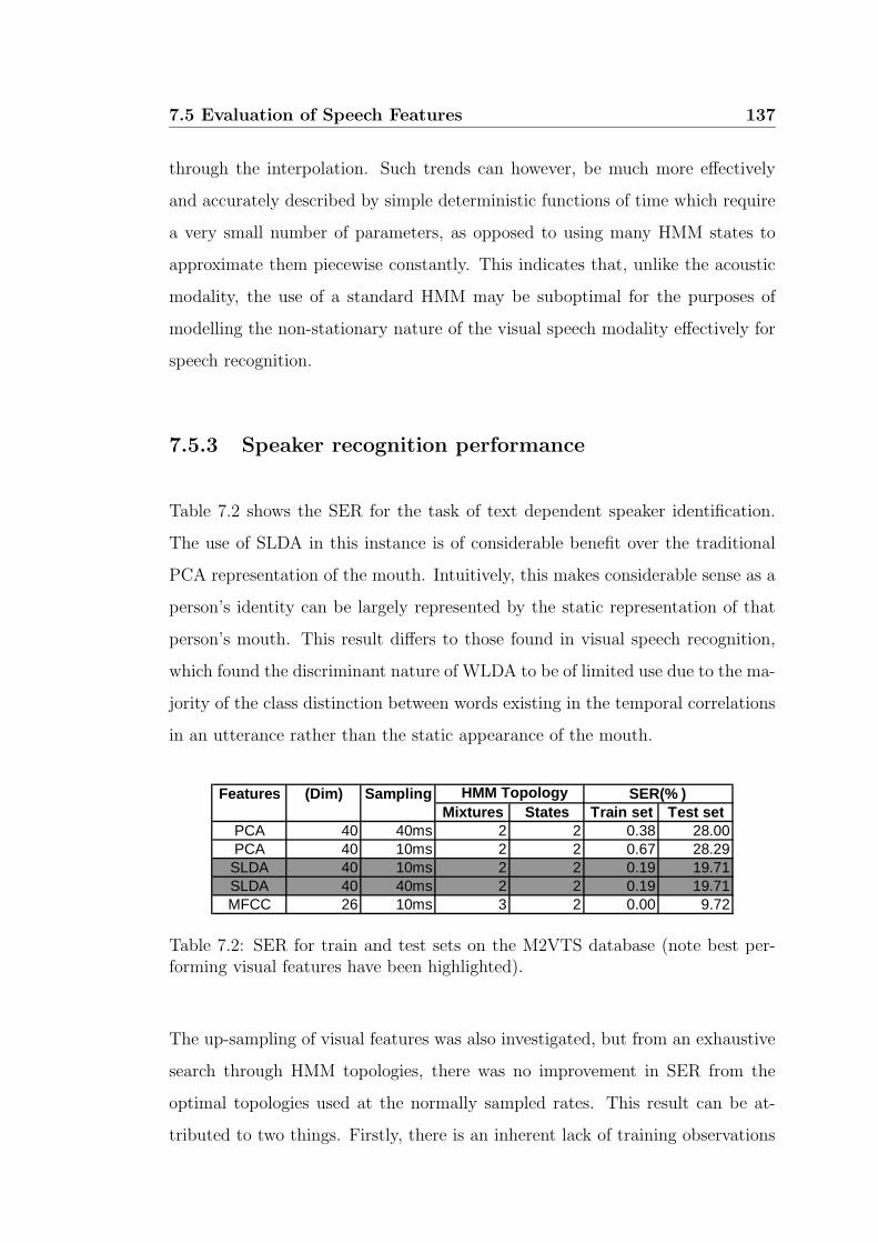
7.5 Evaluation of Speech Features 137
through the interpolation. Such trends can however, be much more effectively
and accurately described by simple deterministic functions of time which require
a very small number of parameters, as opposed to using many HMM states to
approximate them piecewise constantly. This indicates that, unlike the acoustic
modality, the use of a standard HMM may be suboptimal for the purposes of
modelling the non-stationary nature of the visual speech modality effectively for
speech recognition.
7.5.3 Speaker recognition performance
Table 7.2 shows the SER for the task of text dependent speaker identification.
The use of SLDA in this instance is of considerable benefit over the traditional
PCA representation of the mouth. Intuitively, this makes considerable sense as a
person’s identity can be largely represented by the static representation of that
person’s mouth. This result differs to those found in visual speech recognition,
which found the discriminant nature of WLDA to be of limited use due to the ma-
jority of the class distinction between words existing in the temporal correlations
in an utterance rather than the static appearance of the mouth.
Features (Dim) Sampling SER(% )Mixtures States Train set Test set
PCA 40 40ms 2 2 0.38 28.00PCA 40 10ms 2 2 0.67 28.29
SLDA 40 10ms 2 2 0.19 19.71SLDA 40 40ms 2 2 0.19 19.71MFCC 26 10ms 3 2 0.00 9.72
HMM Topology
Table 7.2: SER for train and test sets on the M2VTS database (note best per-forming visual features have been highlighted).
The up-sampling of visual features was also investigated, but from an exhaustive
search through HMM topologies, there was no improvement in SER from the
optimal topologies used at the normally sampled rates. This result can be at-
tributed to two things. Firstly, there is an inherent lack of training observations
138 7.6 Chapter Summary
for generating a subject dependent digit HMM, making the generation of suit-
ably complex HMMs difficult. Secondly, the piece-wise temporal approximation
made by a standard HMM suffices for the task of visual speaker recognition due
to its natural ability to discriminate based on static features, as indicated by the
superior performance of SLDA over PCA features. Interestingly, the performance
of the acoustic and visual classifiers are relatively close, with both classifiers be-
ing marginally undertrained. This result was to be expected due to the lack of
training data associated with each subject and digit.
7.6 Chapter Summary
In this chapter feature extraction techniques for the acoustic and visual speech
modalities, pertaining to the tasks of speech and speaker recognition, were eval-
uated. For the well established field of acoustic speech and speaker recognition,
cepstral features based on mel-scale filter bank energy values were reported to
achieve good results, specifically MFCCs. Steps to gain invariance to train/test
mismatches at a feature level were also entertained with liftering and CMS being
employed for added robustness in noise. In the visual speech modality a number
of mouth representations are available with most techniques being classified as
contour, area or a combination of both. Contour features, although offering some
invariance to lighting and speaker variabilities, were deemed to unstable and un-
reliable for use in an AVSP application. Conversely, area features are quite stable
with their representations are robust to noise and compression artifacts.
For speechreading it was shown that MRPCA mouth features, at an interpolated
sample rate, give superior WERs over all those evaluated. Although, WLDA
features, based on a static discriminant space, perform almost as well, and do not
require interpolation and have a much smaller dimensionality. For both feature
sets the benefit of mean subtraction was shown, with the improved performance
being linked to unwanted subject variabilities being removed. An interesting point

7.6 Chapter Summary 139
was also raised about the validity of using a standard HMM for speech recognition
in the visual modality, as the quasi stationary assumption made for the acoustic
modality does not seem to hold as well in the visual modality. Visual speaker
recognition achieved excellent results using the SLDA mouth feature. This can
be attributed to the more static nature of the speaker recognition task, which
is easily accommodated by the LDA feature extraction procedure and standard
HMM topology.

Chapter 8
Independent Classifier
Combination Theory
8.1 Introduction
The optimal combination of classifiers from independent observation domains has
a myriad of benefits in practical pattern recognition problems, especially AVSP.
Combining the outputs of several classifiers before making the classification deci-
sion, has led to improved performance in many applications [5, 36, 104]. However,
great care has to be taken when combining the outputs of classifiers due to the risk
of catastrophic fusion. Catastrophic fusion occurs when the performance of an
ensemble of combined classifiers is worse than any of the classifiers individually.
Throughout this chapter the terms context and train/test mismatch will be used
extensively. Context is defined [105] as the collection of situations or parameters
that meet the assumptions of the models. The term context is used to describe
the concept that a classifier’s knowledge (ie. ability to make confident decisions)
is restricted by the context it has been trained under. When a change in context
is encountered in testing that differs from what has been seen in training this

142 8.1 Introduction
uncertainty should be represented in the confidence score. This idea is very im-
portant, as effective classifier combination is heavily dependent on the individual
classifiers providing scores representative of how confident one is that the correct
decision has been made. For example, a classifier may be trained using an obser-
vation train set from a clean context (ie. no noise), this same classifier is used
to classify observations using a test set from a noisy context. If the conditional
class density functions found to optimally classify the train set do not generalise
well to the noisy test set then the confidence scores received will be erroneous as
the decisions have been based on the wrong knowledge context.
The importance of context and ability to generalise in the creation of a truly
intelligent classifier can best be expressed in a paragraph by Dreyfus and Dreyfus
pertaining to the current shortcomings in classifiers compared to truly intelligent
entities [106],
The problem here is that the designer has determined, by means of the
architecture of the net (classifier), that certain possible generalisations
will never be found. All this is well and good for toy problems in which
there is no question of what constitutes a reasonable generalisation,
but in real-world situations a large part of human intelligence consists
in generalising in ways that are appropriate to a context. If the de-
signer restricts the net (classifier) to a predefined class of appropriate
responses, the net (classifier) will not have the common sense that
would enable it to adapt to other contexts, as a truly human intelli-
gence would.
At the time of writing1 (1988), the field of pattern recognition was in a stage
of relative infancy, such that a classifier was referred to as a net. Placing the
philosophical ramifications to artificial intelligence of such a statement to one
1Dreyfus and Dreyfus’s paper [106] provided an excellent critique on the two branchingparadigms of artificial intelligence (AI) and made comment on the newly emerging field neuralnetworks with respect to AI.
8.1 Introduction 143
side, the statement paraphrases current problems with modern classifiers and
classifier theory beautifully. For a classifier to be truly useful in the real world, as
opposed to a toy problem, a classifier needs to be able to allow for the possibility
that it may not be able to make a decision when presented with a new context
based on its current knowledge. As will soon be discussed, most classifiers do
not allow for such a possibility resulting in confidence errors and poor classifier
combination performance.
The difference in context between the train and test sets is referred to as a
train/test mismatch. The measure of train/test mismatch is not the physical
difference between the train and test observations sets but a measure of how gen-
eralised the knowledge gained from the train set is, with reference to the unknown
test set. This measure of generalised knowledge is then integrated with the exist-
ing classifier, formed from the train set context, so as to gain a true confidence in
the decision made by the classifier when being used on the test set. This process
is known as classifier exaptation. This differs to classifier adaptation as no class
specific knowledge of the test set is required to adjust the confidence scores. In-
stead the knowledge from the known train set is exploited in the unknown test set
based on a priori information (i.e. measure of generalised knowledge) of where the
decisions are applicable. Through this measure, effective classifier combination
performance can be realised as one has a true estimate of confidence in the deci-
sions made by each classifier. Using this understanding, a number of combination
strategies can be undertaken to dampen the effects of train/test mismatches and
gain superior classification performance for practical applications; such as those
found in many AVSP applications.
This chapter is divided into a number of sections where in Section 8.4, the
train/test mismatch framework is proposed. A theoretical basis for confidence
error is presented in Section 8.5, with the steps required to calculate and remove
this mismatch error explained. A number of combination functions are then de-
fined in Section 8.6 for use, based on how much quantitative knowledge there is

144 8.2 Bounds for Independent Classifier Combination
about the error. In Section 8.7 added insight is given to the apparent paradox
formed when deciding to adapt or exapt a classifier. Finally 8.8 describes a special
case of adaption found in acoustic cepstral features.
8.2 Bounds for Independent Classifier Combi-
nation
According to Bayesian theory [5], given an observation o with R representa-
tions [o1, . . . ,oR] stemming from R observation domains, and N classes, op-
timal classification should assign the label i∗ as,
i∗ = argN
maxn=1
Pr(ωn|o1, . . . ,oR) (8.1)
Using Bayes theorem one can rewrite the probability Pr(ωi|o1, . . . ,oR) as,
Pr(ωi|o1, . . . ,oR) =
P (ωi)p(o1, . . . ,oR|ωi)
p(o1, . . . ,oR)(8.2)
where P (ωi) is the a priori probability for class ωi, and p(o1, . . . ,oR|ωi) and
p(o1, . . . ,oR) are the class dependent and class independent joint likelihood
functions respectively. Since the denominator in Equation 8.2 is class indepen-
dent, one can concentrate on the numerator. Under the assumption of indepen-
dence between observation domains,
p(o1, . . . ,oR|ωi) =R∏
r=1
p(or|ωi) (8.3)
where p(or|ωi) is the class dependent likelihood function for the rth observation
domain. Using this equivalence one can rewrite the decision rule in Equation 8.1
as,
8.2 Bounds for Independent Classifier Combination 145
i∗ = argN
maxn=1
P (ωn)R∏
r=1
p(or|ωn) (8.4)
or placing in terms of confidence scores,
i∗ = argN
maxn=1
ζ∗pr(ωi|o) (8.5)
where ζ∗pr(ωi|o) is calculated in terms of a posteriori probabilities Pr(ωi|or) and
priors P (ωi) using the product rule Fpr(),
ζ∗pr(ωi|o) = Fpr(Pr(ωi|or),∀r) = P (ωi)
−(R−1)
R∏
r=1
Pr(ωi|or) (8.6)
It must be emphasised that ζ∗pr(ωi|o) is a confidence score (not necessarily be-
tween zero and one), not a probability, but is equivalent to the true probabil-
ity Pr(ωi|o1, . . . ,oR) in terms of the class decision boundaries it realises. For
independent classifiers ζ∗pr(ωi|o) gives an upper bound in classifier combination
performance.
Equation 8.6 holds true if one has access to the true a posteriori probabilities
from all R independent observation domains. In practice however, one can rarely
apply this rule due to the differing decision boundaries realised from the mismatch
between train and test sets. This mismatch results in a confidence error,
P r(ωi|or) = Pr(ωi|o
r) + εi(or) (8.7)
In practice one can only ever apply the product rule Fpr() to the a posteriori prob-
ability estimates P r(ωi|o), resulting in the confidence score estimate ζpr(ωi|o). In
the presence of large confidence errors the estimated confidence score ζpr(ωi|o)
may realise different decision boundaries to the optimal ζ∗pr(ωi|o) resulting in
146 8.3 Exaptation vs. Adaptation
suboptimal classifier combination performance.
The task of effective classifier combination is to judiciously choose combination
strategies F () so as to dampen the effects of confidence errors and give a confi-
dence score ζ(ωi|o) that approximates the optimal decision boundaries realised
by ζ∗pr(ωi|o). If due care is not taken to choose an appropriate combination
function F () an effect known as catastrophic fusion may occur causing the classi-
fication performance of ζ(ωi|o) to fall below ζ∗cf (ωi|o), where ζ∗cf is the confidence
score from the single observation domain with best classification performance in
the test context. The confidence scores ζ∗cf (ωi|o) and ζ∗pr(ωi|o) define upper and
lower bounds of classification error rate for classifier combination. An effective
combination strategy F () must lie between these two bounds.
8.3 Exaptation vs. Adaptation
In recent work in evolution theory [107], the term exaptation has been used to
explain the amazing way life on earth has evolved through natural selection. The
term exaptation can be defined as the characteristics that arise in one context be-
fore being exploited in another [107]. The concept of exaptation can be extended
to classifier combination theory. When using classifiers in practical scenarios, it is
common to adapt them to new contexts (eg. noisy conditions, different speaker,
different lighting, etc.). Unfortunately, in many scenarios one may have no knowl-
edge concerning the class specific change in context, making suitable adaptation
impossible. Fortunately, the knowledge gained from a well defined context (i.e.
train observation set) can often be used, with some success, on an previously
unseen context (i.e. test observation set) to make a decision. When applied to a
classifier, one can refer to this process as classifier exaptation.
Classifier exaptation is the task of defining a critical region of where the knowledge
gained from the train set is significant without intimate knowledge of the test
8.4 Modelling Train/Test Mismatches 147
set. This is referred to as classifier exaptation, as the knowledge gained from
one context (i.e. the train set) is being exploited in another context (i.e. the
test set), without any class specific knowledge from the test set. The main
purpose of exaptation, with reference to classifier combination, is the dampening
of confidence errors caused by the mismatch between train and test sets. Classifier
exaptation, unlike adaptation, does not in practice violate causality (i.e. access
to the test set before testing). This makes classifier exaptation a viable way to
treat the real world problem of making a decision in a previously unseen context.
8.4 Modelling Train/Test Mismatches
The idea of a train/test mismatch can be formally described if one analyses
the problem of determining an a posteriori probability in terms of sets. The
observation o exists in the set Sall such that o ∈ Sall. At any given time, one only
has at their disposal observations existing in the subset Strn ⊂ Sall or Stst ⊂ Sall,
representing training and testing observations respectively. When one has to gain
an a posterior probability estimate P r(ωi|o) of observation o ∈ Ststi, one has
to make a decision based on knowledge gained from observations lying in Strni
even though o may not. A depiction of this situation is shown in the Venn
diagram in Figure 8.1(b) where Sall, Strn and Stst are subsets. Within a Bayesian
framework, one has to allow for the possibility that o 6∈ Strn even though o ∈ Stst.
Using Bayes [35] rule, when different train/test conditions are encountered, one
would ideally use likelihoods p(o|Ststi) derived from our knowledge of the test
set to gain an a posteriori probability,
Pr(Ststi|o) =P (ωi)p(o|Ststi)
∑Nn=1 P (ωn)p(o|Ststn)
(8.8)
However, due to causality the classifier’s knowledge is always restricted to the
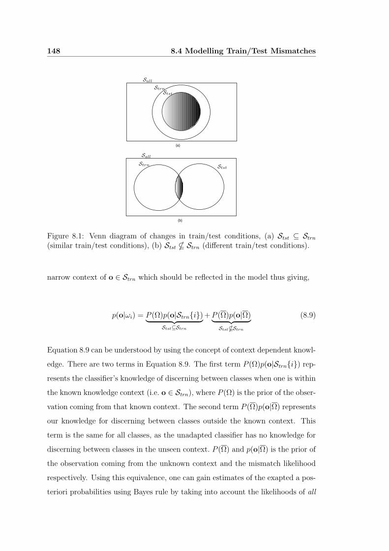
148 8.4 Modelling Train/Test Mismatches
(a)
(b)
PSfrag replacements
Strn
Strn
Stst
Stst
Sall
Sall
Figure 8.1: Venn diagram of changes in train/test conditions, (a) Stst ⊆ Strn
(similar train/test conditions), (b) Stst * Strn (different train/test conditions).
narrow context of o ∈ Strn which should be reflected in the model thus giving,
p(o|ωi) = P (Ω)p(o|Strni)︸ ︷︷ ︸
Stst⊆Strn
+P (Ω)p(o|Ω)︸ ︷︷ ︸
Stst*Strn
(8.9)
Equation 8.9 can be understood by using the concept of context dependent knowl-
edge. There are two terms in Equation 8.9. The first term P (Ω)p(o|Strni) rep-
resents the classifier’s knowledge of discerning between classes when one is within
the known knowledge context (i.e. o ∈ Strn), where P (Ω) is the prior of the obser-
vation coming from that known context. The second term P (Ω)p(o|Ω) represents
our knowledge for discerning between classes outside the known context. This
term is the same for all classes, as the unadapted classifier has no knowledge for
discerning between classes in the unseen context. P (Ω) and p(o|Ω) is the prior of
the observation coming from the unknown context and the mismatch likelihood
respectively. Using this equivalence, one can gain estimates of the exapted a pos-
teriori probabilities using Bayes rule by taking into account the likelihoods of all
8.5 Form of Mismatch Likelihood and Priors 149
classes simultaneously,
Pr(ωi|o) =P (ωi)
[P (Ω)p(o|Strni) + P (Ω)p(o|Ω)
]
∑Nn=1 P (ωn)
[P (Ω)p(o|Strnn) + P (Ω)p(o|Ω)
] (8.10)
under similar train/test conditions one can make the assumption,
P (Ω)p(o|Strnn) P (Ω)p(o|Ω) 1 ≤ n ≤ N (8.11)
which leads to the commonly used estimate,
P r(ωi|o) =P (ωi)p(o|Strni)
∑Nn=1 P (ωn)p(o|Strnn)
.= Pr(Strni|o) (8.12)
Unfortunately, in practice it is infeasible to gain a model of P (Ω) and p(o|Ω),
as one requires intimate knowledge of Strn and Stst a priori. However, one can
see that if Equation 8.12 is applied when Equation 8.11 does not hold (ie. in
the case of external noise or an under trained classifier) the resultant a posteriori
probabilities will be ill-scaled, due to the mismatch class being ignored. This
results in a confidence error εi(o) as first mentioned in Equation 8.7.
Nothing can be done about this error εi(o) when dealing with a single modality
with respect to classification error. However, by suitably scaling P r(ωi|o) one
can convert the mismatch error into Bayesian error, which is intrinsically part
of Pr(ωi|o), allowing for the optimal use of the product rule.
8.5 Form of Mismatch Likelihood and Priors
It is very difficult to parametrically gain a model for p(o|Ω) and its prior P (Ω)
as they are intrinsically dependent on the decision boundaries, formed as a con-
sequence of the interaction of Pr(Strni|o) and Pr(Ststi|o) for all i. However,
150 8.5 Form of Mismatch Likelihood and Priors
in the event of having a priori knowledge of Strn and Stst, one can define the a
posteriori probability of a mismatch as,
Pr(Ω|o) = 1 −N∑
n=1
Pr(Sbthn|o) (8.13)
where,
Pr(Sbthi|o) = Pr(Strni ∩ Ststi|o)
= Pr(Strni|o)Pr(Ststi|Strni,o)(8.14)
Using our knowledge of conditional probability [108] for two sets A and B,
If A ⊂ B then Pr(B|A) = 1
If B ⊂ A then Pr(B|A) = Pr(B)/Pr(A)
If A and B are disjoint then Pr(B|A) = 0
(8.15)
one can define,
Pr(Ststi|Strni,o) =
1, If ηΩ(o) > 1
ηΩ(o), otherwise(8.16)
where,
ηΩ(o) =Pr(Ststi|o)
Pr(Strni|o)(8.17)
Applying this to Equation 8.10, using a posteriori probabilities instead of likeli-
hoods, one can define,
Pr(ωi|o) =[1 − Pr(Ω|o)
]Pr(Strni|o) + P (ωi)Pr(Ω|o) (8.18)
8.5 Form of Mismatch Likelihood and Priors 151
Using Equation 8.10 one can then calculate the mismatch likelihood p(o|Ω), where
the prior P (Ω) = 1 − P (Ω) can be interpreted as the proportion of o 6∈ Sbthi,
for all i.
8.5.1 Synthetic example
In this section a simple synthetic example is proposed to show the benefit of the
train/test mismatch framework to classifier combination theory. In this exam-
ple there are R independent observation domains of dimensionality D = 2. A
dimensionality of two was chosen so as to allow for graphical visualisation and
cater for non-linear decision boundaries. For simplicity each domain r has two
classes ω1 and ω2 described by Gaussian likelihood functions with equal priors.
Again for simplicity and the ability for seeing the effects of varying R, the likeli-
hood functions have the same parametric form for all domains. Each conditional
class density function can be parametrically described by,
p(or|ωi) = N(µi,Σi)|or (8.19)
where r is the observation domain, ωi is the class, µi is the class mean, and Σi
is the class covariance matrix. In each observation domain the observation train
sets Strn1 and Strn2 are described by the parameters,
µ1 = [−2.5, 2.5]T ,µ2 = [2.5,−2.5]T
Σ1 =
2 0
0 1
,Σ2 =
1.5 −0.5
−0.5 1.5
A train/test mismatch was introduced in this example, through the shifting of
model means, so that the observation test sets Stst1 and Stst2 are described
by the parameters,
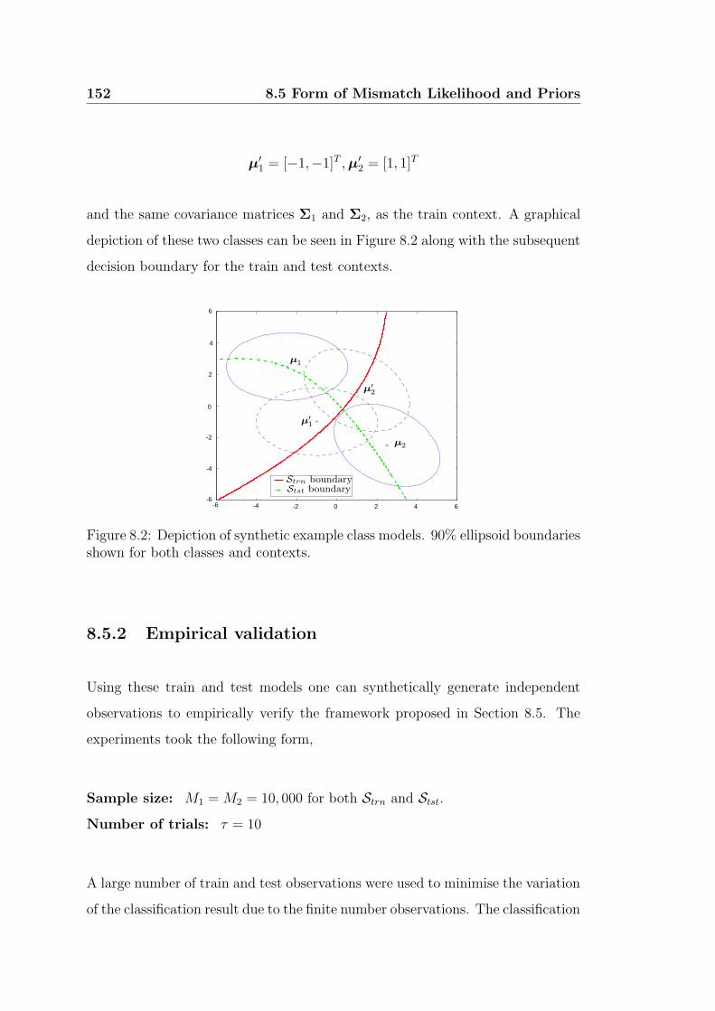
152 8.5 Form of Mismatch Likelihood and Priors
µ′1 = [−1,−1]T ,µ′
2 = [1, 1]T
and the same covariance matrices Σ1 and Σ2, as the train context. A graphical
depiction of these two classes can be seen in Figure 8.2 along with the subsequent
decision boundary for the train and test contexts.
-2-4-6-6
0 2 4 6
-4
-2
0
2
4
6
PSfrag replacements
o1
o2
oslice
µ1
µ2
µ′1
µ′2
Strn boundaryStst boundary
Figure 8.2: Depiction of synthetic example class models. 90% ellipsoid boundariesshown for both classes and contexts.
8.5.2 Empirical validation
Using these train and test models one can synthetically generate independent
observations to empirically verify the framework proposed in Section 8.5. The
experiments took the following form,
Sample size: M1 = M2 = 10, 000 for both Strn and Stst.
Number of trials: τ = 10
A large number of train and test observations were used to minimise the variation
of the classification result due to the finite number observations. The classification
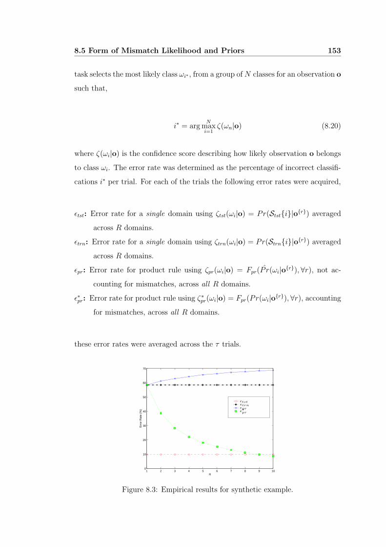
8.5 Form of Mismatch Likelihood and Priors 153
task selects the most likely class ωi∗ , from a group ofN classes for an observation o
such that,
i∗ = argN
maxi=1
ζ(ωn|o) (8.20)
where ζ(ωi|o) is the confidence score describing how likely observation o belongs
to class ωi. The error rate was determined as the percentage of incorrect classifi-
cations i∗ per trial. For each of the trials the following error rates were acquired,
εtst: Error rate for a single domain using ζtst(ωi|o) = Pr(Ststi|or) averaged
across R domains.
εtrn: Error rate for a single domain using ζtrn(ωi|o) = Pr(Strni|or) averaged
across R domains.
εpr: Error rate for product rule using ζpr(ωi|o) = Fpr(P r(ωi|or),∀r), not ac-
counting for mismatches, across all R domains.
ε∗pr: Error rate for product rule using ζ∗pr(ωi|o) = Fpr(Pr(ωi|or),∀r), accounting
for mismatches, across all R domains.
these error rates were averaged across the τ trials.
1 2 3 4 5 6 7 8 9 100
10
20
30
40
50
60
70
R
Err
or R
ate
(%)
PSfrag replacements
εprε∗pr
εtrn
εtst
Figure 8.3: Empirical results for synthetic example.
154 8.5 Form of Mismatch Likelihood and Priors
The results for these different error rates can be seen in Figure 8.3. One can
see the parametric forms of p(o|Strni) and p(o|Ststi) were chosen specifically
to cause catastrophic fusion using the product rule. Catastrophic fusion occurs
when the performance of an ensemble of combined classifiers is worse than any of
those classifiers individually. In Figure 8.3 it can be seen that as R increases, the
error rate of εpr increases from the average train set error εtrn for a single domain.
However, taking the mismatch into account the error rate of ε∗pr decreases as R
increases. It is interesting to note that the performance of ε∗pr, given enough
independent observation domains, surpasses that of εtst for matched conditions.
It must be emphasised that the classification error for Pr(ωi|o) and P r(ωi|o)
are exactly the same, as predicted in Section 8.5 for equal priors, and shown
empirically for εpr and ε∗pr at R = 1. The mismatch error is not removed with
respect to classification error, but now manifests itself as Bayesian error, which
the product rule can optimally handle. This explains why, given a sufficiently
large R, ε∗pr can actually fall below εtst as classifier theory [35, 109] dictates,
due to the errors being independent the average error shall approach zero as R
approaches infinity.
The scenario for unequal priors can also be investigated by changing the priors of
the two classes to P (ω1) = 0.7 and P (ω2) = 0.3 making the number of observation
samples for each class N1 = 14, 000 and N2 = 6, 000 respectively. The empirical
results were obtained using τ = 10 trials for this new experiment with the results
being seen in Figure 8.4. In this scenario, one can see the classification
error for Pr(ωi|o) and P r(ωi|o) are not the same, as predicted in Section 8.5 for
unequal priors, as the class priors tend to dominate when the train/test mismatch
becomes large. Again, as predicted in classifier theory, the average error for ε∗pr,
due to the errors being independent, shall tend to zero as R approaches infinity.
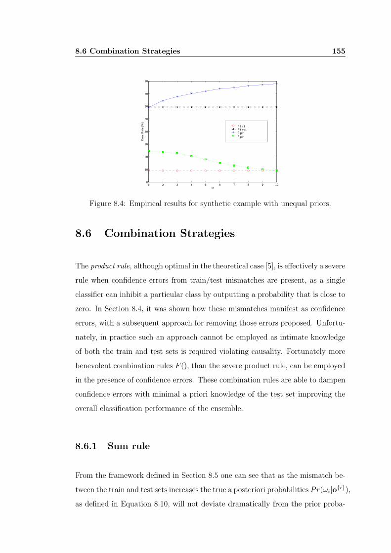
8.6 Combination Strategies 155
1 2 3 4 5 6 7 8 9 100
10
20
30
40
50
60
70
80
R
Err
or R
ate
(%)
PSfrag replacements
εprε∗pr
εtrn
εtst
Figure 8.4: Empirical results for synthetic example with unequal priors.
8.6 Combination Strategies
The product rule, although optimal in the theoretical case [5], is effectively a severe
rule when confidence errors from train/test mismatches are present, as a single
classifier can inhibit a particular class by outputting a probability that is close to
zero. In Section 8.4, it was shown how these mismatches manifest as confidence
errors, with a subsequent approach for removing those errors proposed. Unfortu-
nately, in practice such an approach cannot be employed as intimate knowledge
of both the train and test sets is required violating causality. Fortunately more
benevolent combination rules F (), than the severe product rule, can be employed
in the presence of confidence errors. These combination rules are able to dampen
confidence errors with minimal a priori knowledge of the test set improving the
overall classification performance of the ensemble.
8.6.1 Sum rule
From the framework defined in Section 8.5 one can see that as the mismatch be-
tween the train and test sets increases the true a posteriori probabilities Pr(ωi|or),
as defined in Equation 8.10, will not deviate dramatically from the prior proba-
156 8.6 Combination Strategies
bilities, due to the mismatch likelihood function p(o|Ω) becoming common to all
classes such that,
Pr(ωi|or) = P (ωi)(1 + δir) (8.21)
where δir satisfies δir 1. Kittler [5] called this a strong assumption, however
using the framework of train/test mismatches previously defined in Equation 8.10
it becomes natural due to the inclusion of the mismatch class Ω. Substituting
Equation 8.21 into the original product rule,
P (ωi)−(R−1)
R∏
r=1
Pr(ωi|or) = P (ωi)
R∏
r=1
(1 + δir) (8.22)
If Equation 8.22 is expanded and any terms of second and higher order neglected,
P (ωi)∏R
r=1(1 + δir) ≈ P (ωi) + P (ωi)∑R
r=1 δir
≈ P (ωi) + P (ωi)[−R +∑R
r=1(1 + δir)]
≈ (1 −R)P (ωi) + P (ωi)∑R
r=1(1 + δir)
(8.23)
Substituting Equations 8.23 and 8.21 into 8.6 the sum rule can approximate the
optimal product rule,
Fpr(Pr(ωi|or),∀r) ≈ Fsr(Pr(ωi|o
a),∀r)
≈ (1 −R)P (ωi) +∑R
r=1 Pr(ωi|or)
where, Fsr(Pr(ωi|or),∀r)
.= (1 −R)P (ωi) +
∑Rr=1 Pr(ωi|o
r)
(8.24)
The benefit of this approximation comes to fruition in the practical case when
the estimated a posteriori probabilities P r(ωi|or) are used. Substituting the
confidence errors P r(ωi|or) = Pr(ωi|o
r) + εi(or) defined in Equation 8.7
into the product rule,
8.6 Combination Strategies 157
Fpr(P r(ωi|or),∀r) = P (ωi)
−(R−1)
R∏
r=1
[Pr(ωi|or) + εi(o
r)] (8.25)
From Equations 8.7 and 8.18 the confidence error εi(or) can be defined as,
εi(or) = [P r(ωi|o
r) − P (ωi)]Pr(Ω|o) (8.26)
Inspecting Equation 8.26 one can make the assumption that in the presence of a
train/test mismatch εi(or) Pr(ωi|o
r). Secondly, as the mismatch likelihood
function p(o|Ω) becomes common to all classes, as defined in Equation 8.10, an
assumption that Pr(ωi|or) 6= 0 can be made. Based on these two assumptions
the product term of Equation 8.25 can be rearranged as,
R∏
r=1
[Pr(ωi|or) + εi(o
r)] =
[R∏
r=1
Pr(ωi|or)
]R∏
r=1
[
1 +εi(o
r)
Pr(ωi|or)
]
(8.27)
which can be linearized [5] as
R∏
r=1
[Pr(ωi|or) + εi(o
r)] =
[R∏
r=1
Pr(ωi|or)
][
1 +R∑
r=1
εi(or)
Pr(ωi|or)
]
(8.28)
Comparing Equations 8.6 and 8.28 it is apparent that each term in the error free
product rule is affected by error factor,
1 +R∑
r=1
εi(or)
Pr(ωi|or)(8.29)
Similarly for the sum rule with confidence errors,
Fsr(P r(ωi|or),∀r) = (1 −R)P (ωi)
R∑
r=1
[Pr(ωi|o
r) + εi(or)
](8.30)

158 8.6 Combination Strategies
one can rearrange the sum term in Equation 8.30 as,
R∑
r=1
[Pr(ωi|or) + εi(o
r)] =
[R∑
r=1
Pr(ωi|or)
][
1 +
∑Rr=1 εi(o
r)∑R
r=1 Pr(ωi|or
]
(8.31)
Comparing Equations 8.24 and 8.31 it is apparent that each term in the error
free sum rule is affected by error factor,
1 +
∑Rr=1 εi(o
r)∑R
r=1 Pr(ωi|or(8.32)
By comparing error factors in Equations 8.29 and 8.32 for the product and sum
rules respectively, the sensitivity of the product rule to error is far more dramatic
than the sum rule. Kittler [5] pointed out, that since the a posteriori class proba-
bilities are less than unity, each error in Equation 8.29 is amplified by 1Pr(ωi|or)
.
Conversely for the sum rule, each error in Equation 8.32 is scaled by the sum of
the a posteriori probabilities. For the most probable class, this sum is likely to
be greater than one which will result in the dampening of errors.
8.6.2 Other combination strategies
The product and sum rules constitute the basic schemes for classifier combination.
From these two rules, many commonly used classifier combination strategies can
be developed [5] noting that,
R∏
r=1
Pr(ωi|or) ≤
R
minr=1
Pr(ωi|or) ≤
1
R
∑
r=1
Pr(ωi|or) ≤
Rmaxr=1
Pr(ωi|or)
(8.33)
Equation 8.33 suggests that the product and sum rules can be approximated by
the min and max rules as defined by the lower and upper bounds respectively.
8.6 Combination Strategies 159
Additionally, the hardening of the a posteriori probabilities Pr(ωi|or) to pro-
duce binary valued functions ∆ir as
∆ir =
1 if Pr(ωi|or) = maxN
n=1 Pr(ωn|or)
0 otherwise(8.34)
results in combining decision outcomes rather than combining a posteriori prob-
abilities. This type of hardening is especially useful when the confidence scores
from a classifier are not representative of the true a posteriori probabilities, but
the order of scores is representative of the order of the true a posteriori probabil-
ities.
Max Rule: approximating the sum rule with the max operator as per Equa-
tion 8.33 one can obtain,
ζmxr(ωi|o) = (1 −R)P (ωi) +RR
maxr=1
Pr(ωi|or) (8.35)
Min Rule: approximating the product rule with the min operator as per Equa-
tion 8.33 one can obtain,
ζmnr(ωi|o) = P (ωi)−(R−1)
R
minr=1
Pr(ωi|or) (8.36)
Median Rule: Under the assumption of equal priors the sum rule can be viewed
as computing the mean of a posteriori probabilities across R observation
domains. If any of the classifiers outputs an a posteriori probability for
some class which is an outlier, it will affect the average. A well known
approach to combat such occurrences is to take the median rather than
mean, leading to,
ζmdr(ωi|o) = medRr=1Pr(ωi|o
r) (8.37)
Majority Vote Rule: Using the sum rule, assuming equal priors and by hard-
ening the a posteriori probabilities according to Equation 8.34 one can for-
mulate,
160 8.6 Combination Strategies
ζmvr(ωi|o) =R∑
r=1
∆ir (8.38)
The rules expressed in Equations 8.35 to 8.38, in a similar manner to the sum
rule, try to approximate the confidence score of the error free product rule. The
choice of rule is heavily dependent on the nature of the task, type of classifier
and the mismatch being dealt with. For most of the experimental work in this
thesis the rules in Equations 8.35 to 8.38 will not be used. This is partly due to
the clear theoretical mathematical relationship the sum rule has to the error free
product rule as opposed to the heuristically sound approximations outlined here
in Equations 8.35 to 8.38. Additionally, the parametric classifiers used through-
out the experimental work in this thesis are able to give accurate approximations
to p(o|Strni) making many of the approximations made in this section unnec-
essary.
8.6.3 Weighted product rule
The empirical benefit of the weighted product rule, in dampening confidence er-
rors, has been well documented [20, 24] in practical AVSP applications. Although
empirically justified there has been minimal work done to understand the under-
lying theory behind such a combination strategy. In this section the weighted
product rule is derived theoretically from within the framework of train/test mis-
matches.
When one has to make a decision between two classes ωi and ωj based on the
combination of R classifiers from R independent observation domains, given
that Stst ⊆ Strn such that P r(ωi|or) ≈ Pr(ωi|o
r), the following optimal deci-

8.6 Combination Strategies 161
sion rule is obtained,
Fpr(P r(ωi|or),∀r)
ωj
≶
ωi
Fpr(P r(ωj|or),∀r) where i 6= j (8.39)
However if a train/test mismatch occurs such that Stst * Strn using Equa-
tions 8.10 the following decision rule eventuates in terms of priors and likelihoods,
P (ωi)R∏
r=1
pir + dr
ωj
≶
ωi
P (ωj)R∏
r=1
pjr + dr where i 6= j (8.40)
to simplify notation pir = p(or|Strni) and dr = P (Ωr)−1P (Ωr
)p(or|Ω).
Using the identity,
pir + dr
pjr + dr
=
(pir
pjr
)βr
(8.41)
where,
βr =log(pir + dr) − log(pjr + dr)
log(pir) − log(pjr)(8.42)
results in the new decision rule,
P (ωi)R∏
r=1
(pir)βr
ωj
≶
ωi
P (ωj)R∏
r=1
(pjr)βr where i 6= j (8.43)
The decision rule in Equation 8.43 can be rewritten purely in terms of the es-
timated a posteriori probability P r(ωi|or), prior P (ωi), and an exponential
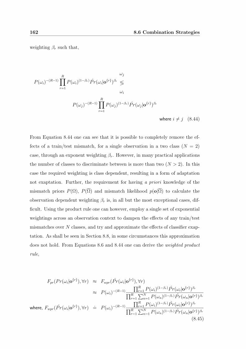
162 8.6 Combination Strategies
weighting βr such that,
P (ωi)−(R−1)
R∏
r=1
P (ωi)(1−βr)P r(ωi|o
r)βr
ωj
≶
ωi
P (ωj)−(R−1)
R∏
r=1
P (ωj)(1−βr)P r(ωj|o
r)βr
where i 6= j (8.44)
From Equation 8.44 one can see that it is possible to completely remove the ef-
fects of a train/test mismatch, for a single observation in a two class (N = 2)
case, through an exponent weighting βr. However, in many practical applications
the number of classes to discriminate between is more than two (N > 2). In this
case the required weighting is class dependent, resulting in a form of adaptation
not exaptation. Further, the requirement for having a priori knowledge of the
mismatch priors P (Ω), P (Ω) and mismatch likelihood p(o|Ω) to calculate the
observation dependent weighting βr is, in all but the most exceptional cases, dif-
ficult. Using the product rule one can however, employ a single set of exponential
weightings across an observation context to dampen the effects of any train/test
mismatches over N classes, and try and approximate the effects of classifier exap-
tation. As shall be seen in Section 8.8, in some circumstances this approximation
does not hold. From Equations 8.6 and 8.44 one can derive the weighted product
rule,
Fpr(Pr(ωi|or),∀r) ≈ Fwpr(P r(ωi|o
r),∀r)
≈ P (ωi)−(R−1)
∏Rr=1 P (ωi)
(1−βr)P r(ωi|or)βr
∏Rr=1
∑Nn=1 P (ωn)(1−βr)P r(ωn|or)βr
where, Fwpr(P r(ωi|or),∀r)
.= P (ωi)
−(R−1)
∏Rr=1 P (ωi)
(1−βr)P r(ωi|or)βr
∏Rr=1
∑Nn=1 P (ωn)(1−βr)P r(ωn|or)βr
(8.45)
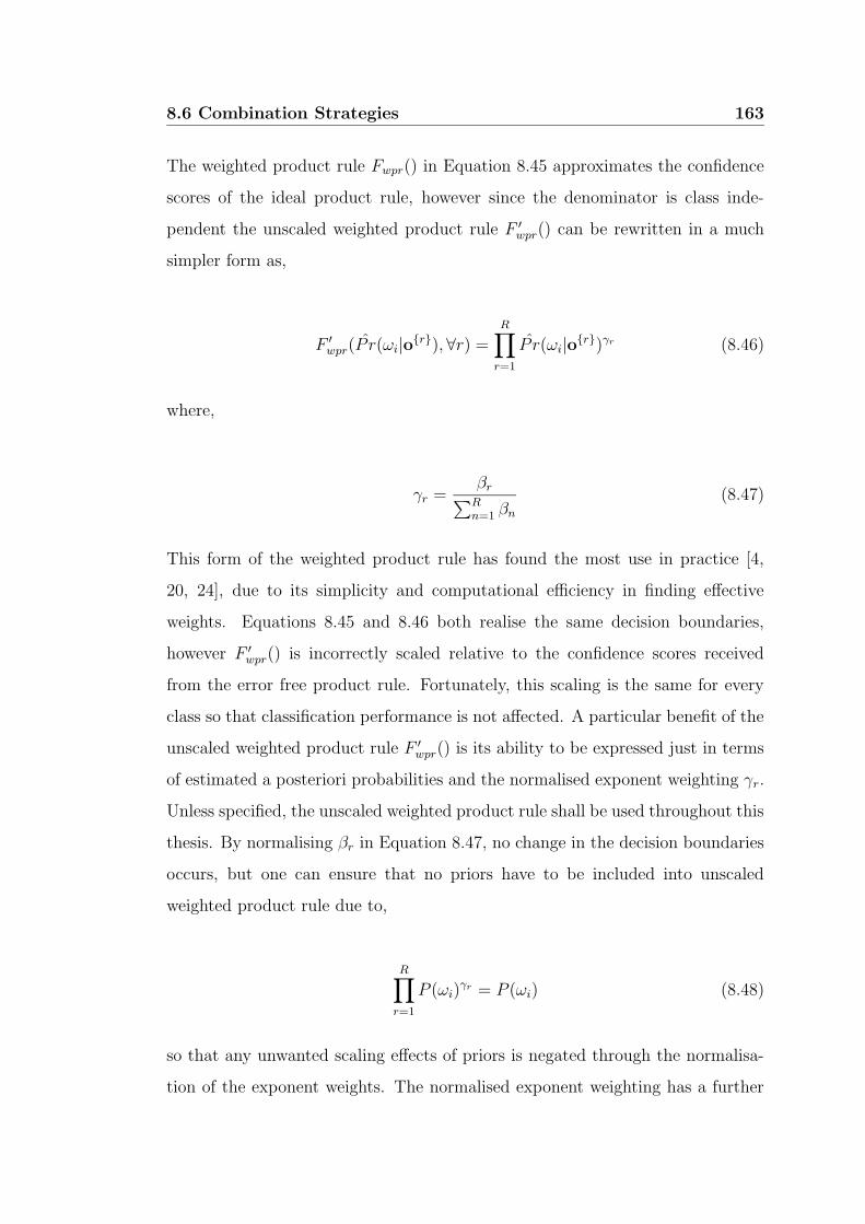
8.6 Combination Strategies 163
The weighted product rule Fwpr() in Equation 8.45 approximates the confidence
scores of the ideal product rule, however since the denominator is class inde-
pendent the unscaled weighted product rule F ′wpr() can be rewritten in a much
simpler form as,
F ′wpr(P r(ωi|o
r),∀r) =R∏
r=1
P r(ωi|or)γr (8.46)
where,
γr =βr
∑Rn=1 βn
(8.47)
This form of the weighted product rule has found the most use in practice [4,
20, 24], due to its simplicity and computational efficiency in finding effective
weights. Equations 8.45 and 8.46 both realise the same decision boundaries,
however F ′wpr() is incorrectly scaled relative to the confidence scores received
from the error free product rule. Fortunately, this scaling is the same for every
class so that classification performance is not affected. A particular benefit of the
unscaled weighted product rule F ′wpr() is its ability to be expressed just in terms
of estimated a posteriori probabilities and the normalised exponent weighting γr.
Unless specified, the unscaled weighted product rule shall be used throughout this
thesis. By normalising βr in Equation 8.47, no change in the decision boundaries
occurs, but one can ensure that no priors have to be included into unscaled
weighted product rule due to,
R∏
r=1
P (ωi)γr = P (ωi) (8.48)
so that any unwanted scaling effects of priors is negated through the normalisa-
tion of the exponent weights. The normalised exponent weighting has a further
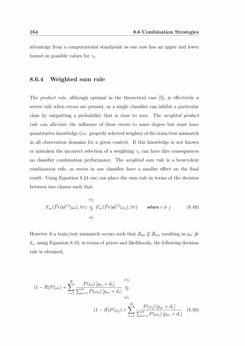
164 8.6 Combination Strategies
advantage from a computational standpoint as one now has an upper and lower
bound on possible values for γr.
8.6.4 Weighted sum rule
The product rule, although optimal in the theoretical case [5], is effectively a
severe rule when errors are present, as a single classifier can inhibit a particular
class by outputting a probability that is close to zero. The weighted product
rule can alleviate the influence of these errors to some degree but must have
quantitative knowledge (i.e. properly selected weights) of the train/test mismatch
in all observation domains for a given context. If this knowledge is not known
or mistaken the incorrect selection of a weighting γr can have dire consequences
on classifier combination performance. The weighted sum rule is a benevolent
combination rule, as errors in one classifier have a smaller effect on the final
result. Using Equation 8.24 one can place the sum rule in terms of the decision
between two classes such that,
Fsr(P r(or|ωi),∀r)
ωj
≶
ωi
Fsr(P r(or|ωj),∀r) where i 6= j (8.49)
However if a train/test mismatch occurs such that Stst * Strn resulting in pir 6
dr, using Equation 8.10, in terms of priors and likelihoods, the following decision
rule is obtained,
(1 −R)P (ωi) +R∑
r=1
P (ωi) [pir + dr]∑N
n=1 P (ωn) [pnr + dr]
ωj
≶
ωi
(1 −R)P (ωj) +R∑
r=1
P (ωj) [pjr + dr]∑N
n=1 P (ωn) [pnr + dr](8.50)
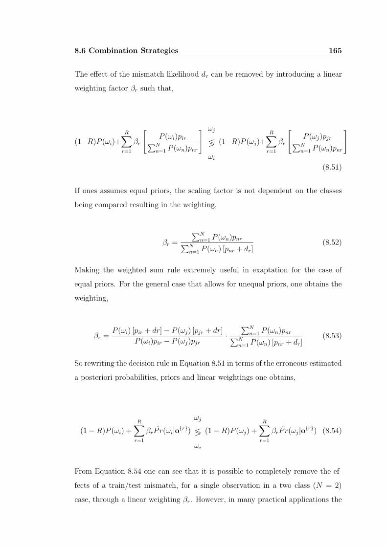
8.6 Combination Strategies 165
The effect of the mismatch likelihood dr can be removed by introducing a linear
weighting factor βr such that,
(1−R)P (ωi)+R∑
r=1
βr
[
P (ωi)pir∑N
n=1 P (ωn)pnr
] ωj
≶
ωi
(1−R)P (ωj)+R∑
r=1
βr
[
P (ωj)pjr∑N
n=1 P (ωn)pnr
]
(8.51)
If ones assumes equal priors, the scaling factor is not dependent on the classes
being compared resulting in the weighting,
βr =
∑Nn=1 P (ωn)pnr
∑Nn=1 P (ωn) [pnr + dr]
(8.52)
Making the weighted sum rule extremely useful in exaptation for the case of
equal priors. For the general case that allows for unequal priors, one obtains the
weighting,
βr =P (ωi) [pir + dr] − P (ωj) [pjr + dr]
P (ωi)pir − P (ωj)pjr
·
∑Nn=1 P (ωn)pnr
∑Nn=1 P (ωn) [pnr + dr]
(8.53)
So rewriting the decision rule in Equation 8.51 in terms of the erroneous estimated
a posteriori probabilities, priors and linear weightings one obtains,
(1 −R)P (ωi) +R∑
r=1
βrP r(ωi|or)
ωj
≶
ωi
(1 −R)P (ωj) +R∑
r=1
βrP r(ωj|or) (8.54)
From Equation 8.54 one can see that it is possible to completely remove the ef-
fects of a train/test mismatch, for a single observation in a two class (N = 2)
case, through a linear weighting βr. However, in many practical applications the
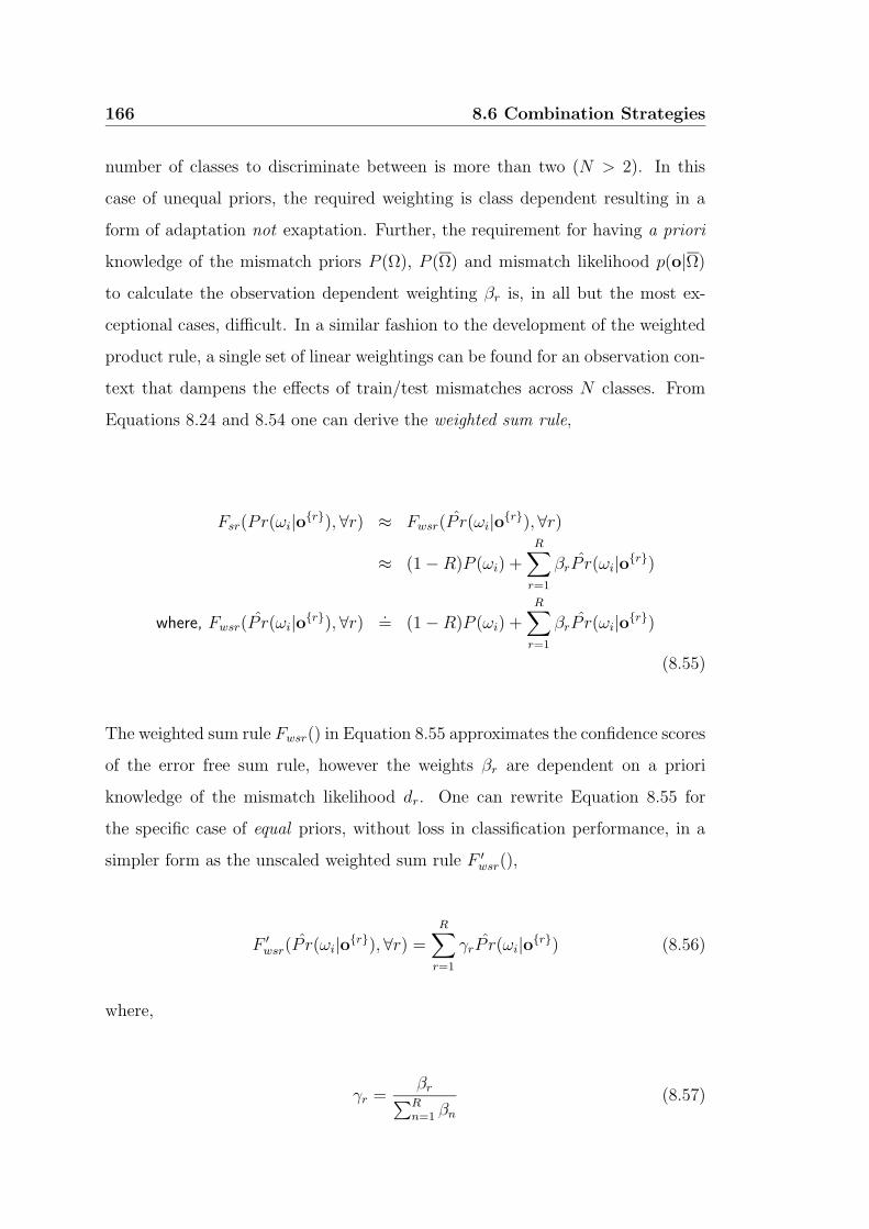
166 8.6 Combination Strategies
number of classes to discriminate between is more than two (N > 2). In this
case of unequal priors, the required weighting is class dependent resulting in a
form of adaptation not exaptation. Further, the requirement for having a priori
knowledge of the mismatch priors P (Ω), P (Ω) and mismatch likelihood p(o|Ω)
to calculate the observation dependent weighting βr is, in all but the most ex-
ceptional cases, difficult. In a similar fashion to the development of the weighted
product rule, a single set of linear weightings can be found for an observation con-
text that dampens the effects of train/test mismatches across N classes. From
Equations 8.24 and 8.54 one can derive the weighted sum rule,
Fsr(Pr(ωi|or),∀r) ≈ Fwsr(P r(ωi|o
r),∀r)
≈ (1 −R)P (ωi) +R∑
r=1
βrP r(ωi|or)
where, Fwsr(P r(ωi|or),∀r)
.= (1 −R)P (ωi) +
R∑
r=1
βrP r(ωi|or)
(8.55)
The weighted sum rule Fwsr() in Equation 8.55 approximates the confidence scores
of the error free sum rule, however the weights βr are dependent on a priori
knowledge of the mismatch likelihood dr. One can rewrite Equation 8.55 for
the specific case of equal priors, without loss in classification performance, in a
simpler form as the unscaled weighted sum rule F ′wsr(),
F ′wsr(P r(ωi|o
r),∀r) =R∑
r=1
γrP r(ωi|or) (8.56)
where,
γr =βr
∑Rn=1 βn
(8.57)

8.6 Combination Strategies 167
By normalising βr in Equation 8.57 no change in the decision boundaries occurs,
but one has an upper and lower bound between one and zero for values of γr.
8.6.5 An elucidative example
In this section, a synthetic example is proposed to show how the various com-
bination strategies perform in the presence of various train/test mismatches. A
synthetic example is used in this section to elucidate the characteristics of the
combination strategies and how they compare to the theoretical upper and lower
error bounds previously defined for independent classifier combination. A sce-
nario of R = 2 independent observation domains was chosen for this example, as
practical applications such as AVSP deal with this problem regularly (i.e. com-
bining the audio and video speech modalities). Additionally, the R = 2 scenario
makes the exhaustive search for weights in the weighted sum and product rules
computationally tractable. A multi-class example (N = 5) is used in this section
where the parametric form of p(o|Strn) and p(o|Ω) is known and is the same for
both observation domains, such that,
p(o|Strni) = N (µi, σ2)|o (8.58)
p(o|Ω) = N (0, σ2Ω)|o (8.59)
where the class means are defined in terms of the class index i,
µi = 2i−N − 1 (8.60)
with a class variance of σ2 = 0.25. The mismatch mean is µΩ = 0 with mis-
match variance of σ2Ω
= 4. A graphical depiction of the train set density func-
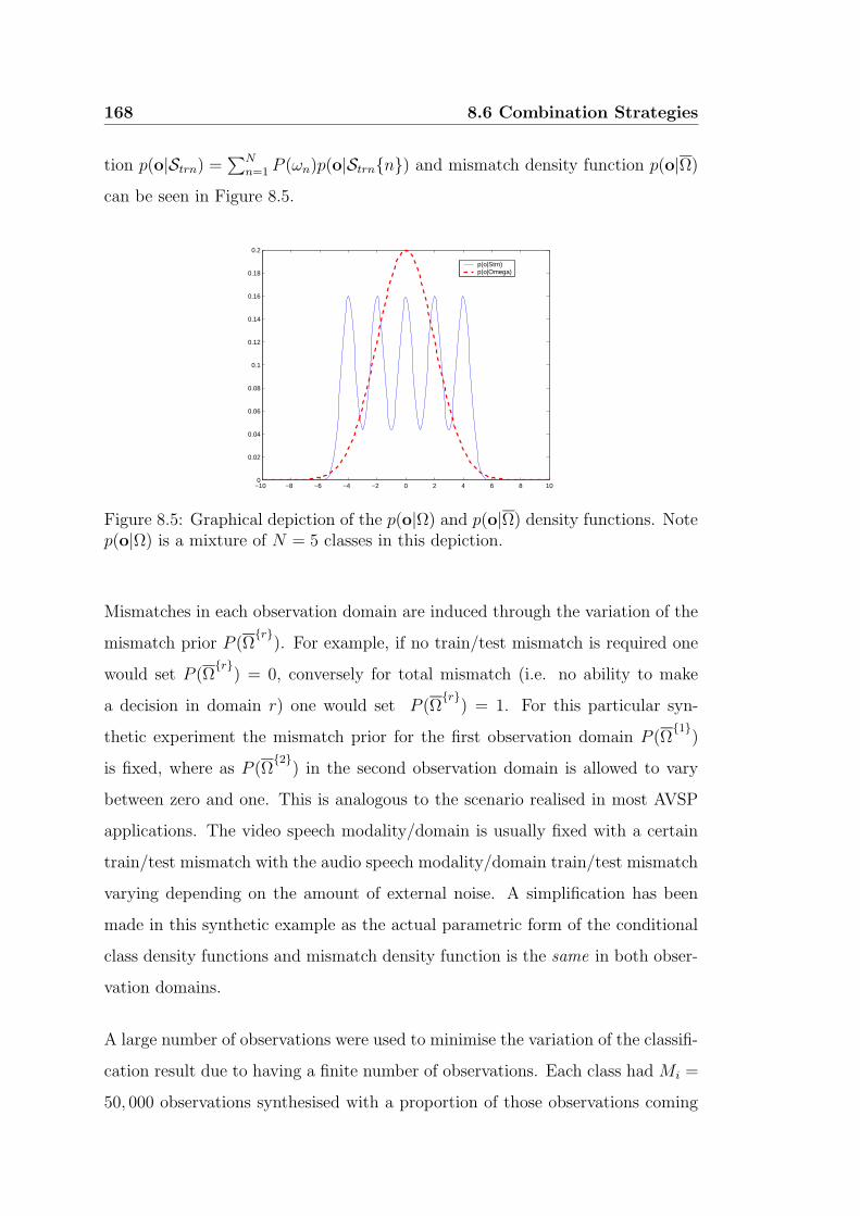
168 8.6 Combination Strategies
tion p(o|Strn) =∑N
n=1 P (ωn)p(o|Strnn) and mismatch density function p(o|Ω)
can be seen in Figure 8.5.
−10 −8 −6 −4 −2 0 2 4 6 8 100
0.02
0.04
0.06
0.08
0.1
0.12
0.14
0.16
0.18
0.2
p(o|Strn)p(o|Omega)
PSfrag replacements
εpr
ε∗pr
εtrn
εtst
Figure 8.5: Graphical depiction of the p(o|Ω) and p(o|Ω) density functions. Notep(o|Ω) is a mixture of N = 5 classes in this depiction.
Mismatches in each observation domain are induced through the variation of the
mismatch prior P (Ωr
). For example, if no train/test mismatch is required one
would set P (Ωr
) = 0, conversely for total mismatch (i.e. no ability to make
a decision in domain r) one would set P (Ωr
) = 1. For this particular syn-
thetic experiment the mismatch prior for the first observation domain P (Ω1
)
is fixed, where as P (Ω2
) in the second observation domain is allowed to vary
between zero and one. This is analogous to the scenario realised in most AVSP
applications. The video speech modality/domain is usually fixed with a certain
train/test mismatch with the audio speech modality/domain train/test mismatch
varying depending on the amount of external noise. A simplification has been
made in this synthetic example as the actual parametric form of the conditional
class density functions and mismatch density function is the same in both obser-
vation domains.
A large number of observations were used to minimise the variation of the classifi-
cation result due to having a finite number of observations. Each class had Mi =
50, 000 observations synthesised with a proportion of those observations coming

8.6 Combination Strategies 169
from the models p(o|Strni) and p(o|Ω) based on the prior P (Ω). In a similar
manner to the synthetic example in Section 8.5.2, for each trial the following error
rates were acquired,
ε1: for the r = 1 observation domain using ζ1(ωi|o) = P r(ωi|o1).
ε2: for the r = 2 observation domain using ζ2(ωi|o) = P r(ωi|o2).
ε∗pr: for error free product rule using ζ∗pr(ωi|o) = Fpr(Pr(ωi|or),∀r).
εpr: for product rule using ζpr(ωi|o) = Fpr(P r(ωi|or),∀r).
εsr: for sum rule using ζsr(ωi|o) = Fsr(P r(ωi|or),∀r).
εwpr: for the weighted product rule using ζwpr(ωi|o) = F ′wpr(P r(ωi|o
r),∀r).
εwsr: for the weighted sum rule using ζwsr(ωi|o) = F ′wsr(P r(ωi|o
r),∀r).
these error rates were averaged across τ = 10 trials. The weightings for the
weighted sum and product rules were found through an exhaustive search of
values between zero and one.
The results for this experiment can be seen in Figure 8.6, with P (Ω1
) = 0.5
being fixed for the first observation domain and P (Ω2
) being varied between
zero and one for the second observation domain. One can clearly see that the
theoretical error free product rule ε∗pr outperforms all other combination strategies
being tested, adding empirical evidence to its use as a lower bound in error for
classification combination performance. The unweighted product rule had very
poor performance εpr in the presence of a train/test mismatch with error rates
above the catastrophic fusion upper bound ε∗cf , defined as ε∗cf = min(ε1, ε2), for all
values of the mismatch prior P (Ω2
), highlighting the severe nature of the rule
when confidence errors are present. As expected, the sum rule εsr fared somewhat
better with error rates below the catastrophic fusion boundary for middle values
of P (Ω2
).
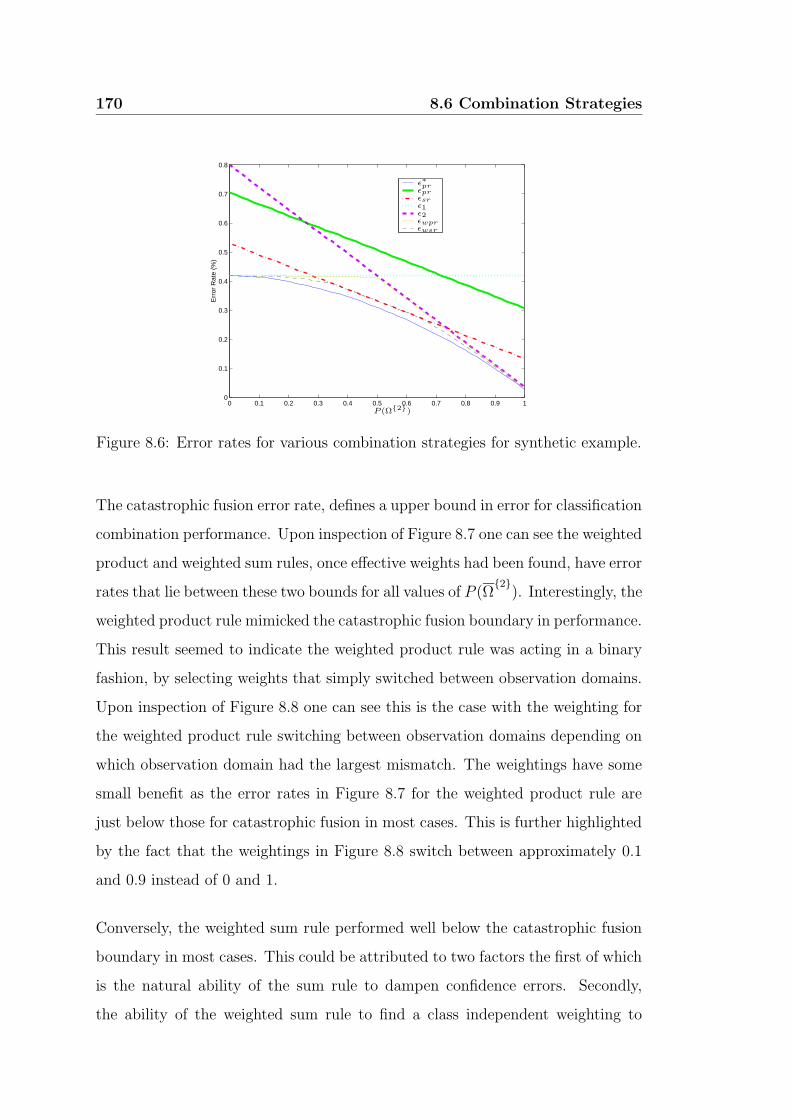
170 8.6 Combination Strategies
0 0.1 0.2 0.3 0.4 0.5 0.6 0.7 0.8 0.9 10
0.1
0.2
0.3
0.4
0.5
0.6
0.7
0.8
Err
or R
ate
(%)
PSfrag replacements
ε∗pr
εsrε1ε2
P (Ω2)
εpr
εwprεwsr
Figure 8.6: Error rates for various combination strategies for synthetic example.
The catastrophic fusion error rate, defines a upper bound in error for classification
combination performance. Upon inspection of Figure 8.7 one can see the weighted
product and weighted sum rules, once effective weights had been found, have error
rates that lie between these two bounds for all values of P (Ω2
). Interestingly, the
weighted product rule mimicked the catastrophic fusion boundary in performance.
This result seemed to indicate the weighted product rule was acting in a binary
fashion, by selecting weights that simply switched between observation domains.
Upon inspection of Figure 8.8 one can see this is the case with the weighting for
the weighted product rule switching between observation domains depending on
which observation domain had the largest mismatch. The weightings have some
small benefit as the error rates in Figure 8.7 for the weighted product rule are
just below those for catastrophic fusion in most cases. This is further highlighted
by the fact that the weightings in Figure 8.8 switch between approximately 0.1
and 0.9 instead of 0 and 1.
Conversely, the weighted sum rule performed well below the catastrophic fusion
boundary in most cases. This could be attributed to two factors the first of which
is the natural ability of the sum rule to dampen confidence errors. Secondly,
the ability of the weighted sum rule to find a class independent weighting to
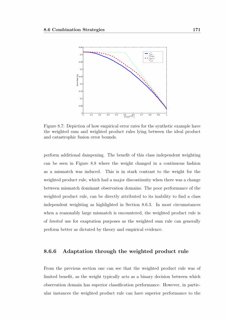
8.6 Combination Strategies 171
0 0.1 0.2 0.3 0.4 0.5 0.6 0.7 0.8 0.9 10
0.05
0.1
0.15
0.2
0.25
0.3
0.35
0.4
0.45
Err
or R
ate
(%)
PSfrag replacements
ε∗pr
P (Ω2)
ε∗cf
εwprεwsr
Figure 8.7: Depiction of how empirical error rates for the synthetic example havethe weighted sum and weighted product rules lying between the ideal productand catastrophic fusion error bounds.
perform additional dampening. The benefit of this class independent weighting
can be seen in Figure 8.8 where the weight changed in a continuous fashion
as a mismatch was induced. This is in stark contrast to the weight for the
weighted product rule, which had a major discontinuity when there was a change
between mismatch dominant observation domains. The poor performance of the
weighted product rule, can be directly attributed to its inability to find a class
independent weighting as highlighted in Section 8.6.3. In most circumstances
when a reasonably large mismatch is encountered, the weighted product rule is
of limited use for exaptation purposes as the weighted sum rule can generally
perform better as dictated by theory and empirical evidence.
8.6.6 Adaptation through the weighted product rule
From the previous section one can see that the weighted product rule was of
limited benefit, as the weight typically acts as a binary decision between which
observation domain has superior classification performance. However, in partic-
ular instances the weighted product rule can have superior performance to the
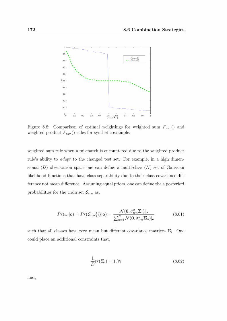
172 8.6 Combination Strategies
0 0.1 0.2 0.3 0.4 0.5 0.6 0.7 0.8 0.9 10
0.1
0.2
0.3
0.4
0.5
0.6
0.7
0.8
0.9
1
PSfrag replacements
Fwpr()Fwsr()
P (Ω2)
γ1
Figure 8.8: Comparison of optimal weightings for weighted sum Fwsr() andweighted product Fwpr() rules for synthetic example.
weighted sum rule when a mismatch is encountered due to the weighted product
rule’s ability to adapt to the changed test set. For example, in a high dimen-
sional (D) observation space one can define a multi-class (N) set of Gaussian
likelihood functions that have class separability due to their class covariance dif-
ference not mean difference. Assuming equal priors, one can define the a posteriori
probabilities for the train set Strn as,
P r(ωi|o).= Pr(Strni|o) =
N (0, σ2trnΣi)|o
∑Nn=1 N (0, σ2
trnΣn)|o(8.61)
such that all classes have zero mean but different covariance matrices Σi. One
could place an additional constraints that,
1
Dtr(Σi) = 1,∀i (8.62)
and,
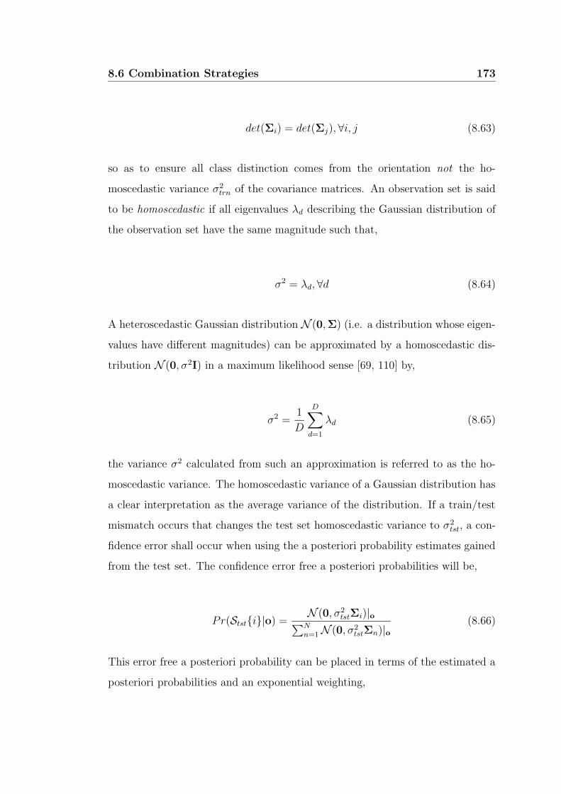
8.6 Combination Strategies 173
det(Σi) = det(Σj),∀i, j (8.63)
so as to ensure all class distinction comes from the orientation not the ho-
moscedastic variance σ2trn of the covariance matrices. An observation set is said
to be homoscedastic if all eigenvalues λd describing the Gaussian distribution of
the observation set have the same magnitude such that,
σ2 = λd,∀d (8.64)
A heteroscedastic Gaussian distribution N (0,Σ) (i.e. a distribution whose eigen-
values have different magnitudes) can be approximated by a homoscedastic dis-
tribution N (0, σ2I) in a maximum likelihood sense [69, 110] by,
σ2 =1
D
D∑
d=1
λd (8.65)
the variance σ2 calculated from such an approximation is referred to as the ho-
moscedastic variance. The homoscedastic variance of a Gaussian distribution has
a clear interpretation as the average variance of the distribution. If a train/test
mismatch occurs that changes the test set homoscedastic variance to σ2tst, a con-
fidence error shall occur when using the a posteriori probability estimates gained
from the test set. The confidence error free a posteriori probabilities will be,
Pr(Ststi|o) =N (0, σ2
tstΣi)|o∑N
n=1 N (0, σ2tstΣn)|o
(8.66)
This error free a posteriori probability can be placed in terms of the estimated a
posteriori probabilities and an exponential weighting,
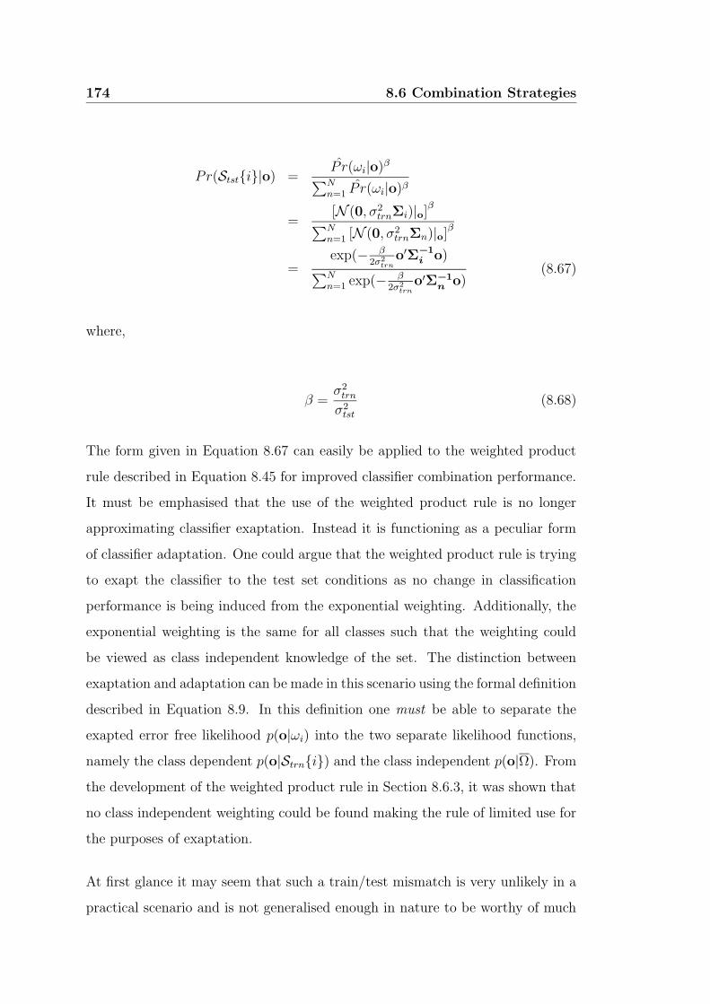
174 8.6 Combination Strategies
Pr(Ststi|o) =P r(ωi|o)β
∑Nn=1 P r(ωi|o)β
=[N (0, σ2
trnΣi)|o]β
∑Nn=1 [N (0, σ2
trnΣn)|o]β
=exp(− β
2σ2trn
o′Σ−1i o)
∑Nn=1 exp(− β
2σ2trn
o′Σ−1n
o)(8.67)
where,
β =σ2
trn
σ2tst
(8.68)
The form given in Equation 8.67 can easily be applied to the weighted product
rule described in Equation 8.45 for improved classifier combination performance.
It must be emphasised that the use of the weighted product rule is no longer
approximating classifier exaptation. Instead it is functioning as a peculiar form
of classifier adaptation. One could argue that the weighted product rule is trying
to exapt the classifier to the test set conditions as no change in classification
performance is being induced from the exponential weighting. Additionally, the
exponential weighting is the same for all classes such that the weighting could
be viewed as class independent knowledge of the set. The distinction between
exaptation and adaptation can be made in this scenario using the formal definition
described in Equation 8.9. In this definition one must be able to separate the
exapted error free likelihood p(o|ωi) into the two separate likelihood functions,
namely the class dependent p(o|Strni) and the class independent p(o|Ω). From
the development of the weighted product rule in Section 8.6.3, it was shown that
no class independent weighting could be found making the rule of limited use for
the purposes of exaptation.
At first glance it may seem that such a train/test mismatch is very unlikely in a
practical scenario and is not generalised enough in nature to be worthy of much
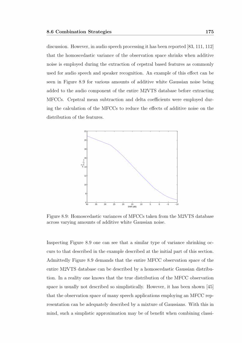
8.6 Combination Strategies 175
discussion. However, in audio speech processing it has been reported [83, 111, 112]
that the homoscedastic variance of the observation space shrinks when additive
noise is employed during the extraction of cepstral based features as commonly
used for audio speech and speaker recognition. An example of this effect can be
seen in Figure 8.9 for various amounts of additive white Gaussian noise being
added to the audio component of the entire M2VTS database before extracting
MFCCs. Cepstral mean subtraction and delta coefficients were employed dur-
ing the calculation of the MFCCs to reduce the effects of additive noise on the
distribution of the features.
−10−505101520253035406
8
10
12
14
16
18
20
22
SNR (dB)
PSfrag replacements
σ2 m
fcc
Figure 8.9: Homoscedastic variances of MFCCs taken from the M2VTS databaseacross varying amounts of additive white Gaussian noise.
Inspecting Figure 8.9 one can see that a similar type of variance shrinking oc-
curs to that described in the example described at the initial part of this section.
Admittedly Figure 8.9 demands that the entire MFCC observation space of the
entire M2VTS database can be described by a homoscedastic Gaussian distribu-
tion. In a reality one knows that the true distribution of the MFCC observation
space is usually not described so simplistically. However, it has been shown [45]
that the observation space of many speech applications employing an MFCC rep-
resentation can be adequately described by a mixture of Gaussians. With this in
mind, such a simplistic approximation may be of benefit when combining classi-
176 8.7 Exaptation or Adaptation, a Paradox?
fier outputs in speech applications. An additional argument will be made in the
next chapter in relation to an actual speech application.
8.7 Exaptation or Adaptation, a Paradox?
From Section 8.5 one can see that it is possible to gain a measure of Pr(Ω|o) and
perform exaptation on a classifier, allowing for the optimal use of the product
rule. However, the theoretical framework presented in Section 8.5 for calculat-
ing Pr(Ω|o) requires intimate knowledge of both the train and test observation
sets. At first glance this type of approach may seem paradoxical. If one has in-
timate knowledge of the test observation set, why not adapt the decision bound-
aries to optimally classify observations for this new context? It can be conceded
that this is a valid point, in most scenarios one should adapt their classifier to
match the decision boundaries realised by the test observation set as this type of
adaptation should equal, if not outperform, any type of classifier exaptation.
In practice however, this is a moot point as one rarely has access to the full test
set. If one did, ideally the test set would then become the train set resulting
in no train/test mismatch and the removal of any subsequent confidence errors.
This is a fundamental problem with classifier adaptation as it requires a violation
of causality (i.e. access to the test set before testing). However, armed with
the knowledge of how confidence errors manifest one can attempt to dampen
their effects through classifier exaptation with no or at least limited quantitative
knowledge of the test set whilst not violating causality. For example, in the ex-
treme case where one has qualitative knowledge that a train/test mismatch has
occurred (i.e. observation is outside critical region of knowledge), but no quan-
titative knowledge on the mismatch, one would employ the unweighted sum rule
or an approximation to it (i.e. median, max or majority rule) due to its natural
ability to dampen the resultant confidence errors. If one had some distance mea-
sure of how far the observation is from the critical region of knowledge, one could
8.8 Defining a Critical Region of Knowledge 177
calculate a weighting for use in the weighted sum rule to provided an additional
avenue for confidence error dampening.
8.8 Defining a Critical Region of Knowledge
Some problems in pattern recognition require the recognition of a single class of
objects among two or more classes when the statistical properties of the other
class or classes is unknown [35, 113]. One often sees this type of problem in person
verification tasks where the likelihood functions of the claimants are known, but
the imposter likelihood functions are not. A similar problem can be found in the
exaptation of a classifier to a train/test mismatch. In this problem one knows the
statistical properties of p(o|Ω) but the form of p(o|Ω) is unknown. The statistical
theory of significance testing is appropriate for dealing with such problems.
On the basis of the likelihood function and other a priori information, one defines
a critical region corresponding to an unlikely event. More specifically, one decides
on some basis that certain values of measurement are unlikely and identifies the
corresponding region in the measurement space. The integral of the likelihood
function over the critical region is the probability of the unlikely event and is
referred to as the significance level of the test. For example, one could define the
critical region so that the unlikely event has probability 0.05; in this case the test
is being carried out at the 5 percent significance level. A typical significance test
can be written in the form,
log p(o|Ω) ≤ Ts (8.69)
where Ts is a significance threshold specifying the significance. This type of
significance testing is a common method for defining such a critical region. This
form of significance test works extremely well when changes from train to test
178 8.8 Defining a Critical Region of Knowledge
conditions cause the distributions of to be centered at different positions called
a translational mismatch. Equation 8.69 is usually a good way of defining a
critical region of significance. This threshold Ts can be thought of as a maximum
distance a given observation can be from the center of the distribution to be still
considered significant.
However, in many applications this type of approach will not work if the train and
test sets are still centered at the same position, but some other type of mismatch
has occurred such as a scale mismatch, where the homoscedastic variance of the
test set has changed from the train set. In real world applications mismatches
are not limited to just translational or scale mismatches, but can take on any
form. However, for purposes of analysis it is often simpler to assume they can be
approximated by some affine transform. Usually this transform is a combination
of translation, scale and rotation, but in some circumstances one type of transform
(i.e. scale) dominates.
Scale mismatch is of particular interest for AVSP, as previously discussed in
Section 8.6.6, as an approximation can be made between this scaling and the
effect white noise has on acoustic speech features. In this scenario, even though
a mismatch has occurred, there is no easy way to define a maximum distance
threshold as no translational shift has occurred. If shrinkage has occurred the
average log-likelihood scores of the test observation set, will on average, be smaller
than that of the train observation set, essentially making Equation 8.69 useless.
In Section 8.6.6 such an example was given where the homoscedastic variance
of the conditional class density functions shrink, but are all still centered at the
same mean. A graphical interpretation of these two types of mismatches can be
seen in Figure 8.10.
When a scale mismatch is encountered, one can actually use the homoscedas-
tic variance estimate as a way to calculate a suitable exponential weighting for
classifier adaptation and to also define a critical region of knowledge past which
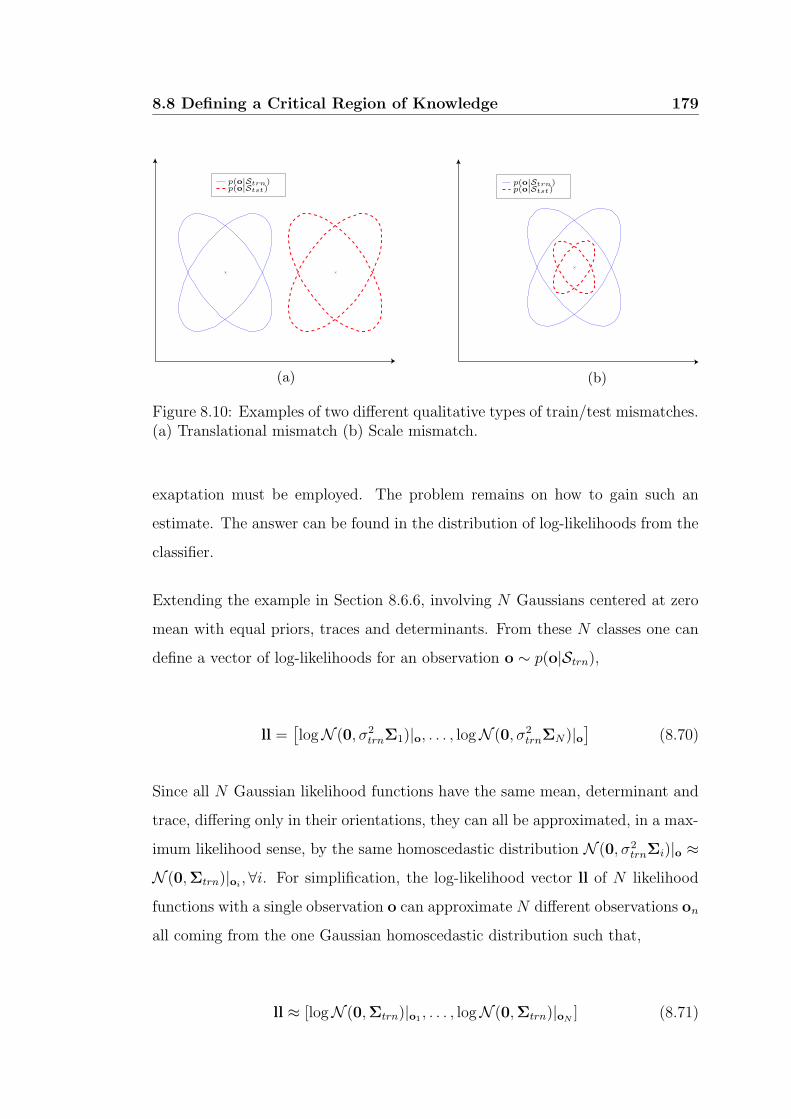
8.8 Defining a Critical Region of Knowledge 179
PSfrag replacements
(a)
(b)(a)
p(o|Strn)p(o|Strn)p(o|Stst)p(o|Stst)
Figure 8.10: Examples of two different qualitative types of train/test mismatches.(a) Translational mismatch (b) Scale mismatch.
exaptation must be employed. The problem remains on how to gain such an
estimate. The answer can be found in the distribution of log-likelihoods from the
classifier.
Extending the example in Section 8.6.6, involving N Gaussians centered at zero
mean with equal priors, traces and determinants. From these N classes one can
define a vector of log-likelihoods for an observation o ∼ p(o|Strn),
ll =[logN (0, σ2
trnΣ1)|o, . . . , logN (0, σ2trnΣN)|o
](8.70)
Since all N Gaussian likelihood functions have the same mean, determinant and
trace, differing only in their orientations, they can all be approximated, in a max-
imum likelihood sense, by the same homoscedastic distribution N (0, σ2trnΣi)|o ≈
N (0,Σtrn)|oi,∀i. For simplification, the log-likelihood vector ll of N likelihood
functions with a single observation o can approximate N different observations on
all coming from the one Gaussian homoscedastic distribution such that,
ll ≈ [logN (0,Σtrn)|o1 , . . . , logN (0,Σtrn)|oN] (8.71)

180 8.8 Defining a Critical Region of Knowledge
According to [35] a set of N observations Otst = [o1, . . . ,oN ]′ of zero mean, drawn
from N (0|Σtrn)|o can be evaluated by a Gaussian distribution,
N (0,Σtrn)|Otst=
1
(2π)D/2|Σtrn|1/2exp(−
1
2d) (8.72)
where Σtrn is the covariance matrix that is thought to describe the covariance
matrix of the N×D matrix of test set observations Otst, which is really described
by Σtst = 1NO′
tstOtst. The N dimensional vector d is described by,
d = diagO′tstΣ
−1trnOtst (8.73)
It can be shown in [35] and formally proven in Appendix A.1 that,
V ard = 2tr[(ΣtstΣ
−1trn)2
](8.74)
Using Equation 8.74 one can see that if there is no train/test mismatch then,
V ard = 2D (8.75)
However, when there is a train/test mismatch then d shall have the following
variance,
V ard = 2Dσ4
tst
σ4trn
(8.76)
Now extending this to the use of log-likelihoods where,
8.9 Chapter Summary 181
ll = ln
[1
(2π)D/2|Σtrn|1/2exp(−
1
2d)
]
= ln
[1
(2π)D/2|Σtrn|1/2
]
−1
2d (8.77)
using Equation 8.76 and 8.77 gives the log-likelihood variance of,
V arll =D
2
σ4tst
σ4trn
(8.78)
From Equation 8.78 it can be seen that the variance of log-likelihood scores
from N Gaussian or approximately Gaussian distributions can be very useful
when a scale mismatch is encountered. In Chapter 9 the importance of this
result to AVSP shall be demonstrated. Admittedly, the accuracy of this vari-
ance measure is highly dependent in practice on the size of N and how well the
homoscedastic approximation holds for the practical problem in question. In
Chapter 9, a practical problem shall be broached demonstrating how a measure
such as log-likelihood variance can be used for classifier adaptation and can also
be used to define a critical region for purposes of classifier exaptation when a
scale mismatch is assumed.
8.9 Chapter Summary
This chapter has presented work concerning the development of a theoretical
framework for independent classifier combination. The product rule, in theory,
was shown to be the optimal combination function for classifiers generated from
independent observation domains. The concept of train/test mismatch was intro-
duced as the root of classifier confidence errors in practice, which subsequently
affect optimal classifier combination performance. Typically classifier adaptation
(i.e. matching the train and test sets) can be employed to remove these confidence

182 8.9 Chapter Summary
errors but is often unviable in practice due to its violation of causality (i.e. has
access to the test set before testing). A novel technique for dampening confidence
errors was developed termed classifier exaptation.
Classifier exaptation differs to adaptation as it takes the characteristics of a clas-
sifier learnt from one context (train set) and exploits them in a new context (test
set), as opposed to matching the test conditions directly. Exaptation is superior
to adaptation in some respects as it does not require class specific knowledge of
the mismatch. This is of particular importance as approximations to classifier
exaptation can be made in practice that do not violate casuality. Different mani-
festations of these approximations were developed based on their knowledge of the
mismatch, such as the sum, median, majority vote, weighted sum and weighted
product rules. Synthetic examples were presented that highlighted the strengths
and weaknesses of such rules in the presence of different mismatches.
A special case for the weighted product rule was also presented, where a specific
type of adaptation as opposed to exaptation occurs. In this special case a scale
mismatch is assumed between the train and test sets, from the classifier log-
likelihoods it was shown that the weighted product rule can alleviate the effects
of such a mismatch. In Chapter 9 the ramifications of this development will be
expanded upon.
Chapter 9
Integration Strategies for
Audio-visual Speech Processing
9.1 Introduction
The effective integration of the acoustic and visual speech modalities in speech
processing is an inherently multidisciplinary field. Audio-visual speech processing
(AVSP) draws on fields as abstract as classifier combination theory in pattern
recognition to the practical study of audio-visual linguistics. Fundamental aspects
of AVSP are analysed in this chapter for the specific tasks of speech recognition
and text dependent speaker recognition, but most aspects can be applied to all
fields of AVSP and pattern recognition in general.
In this chapter an in depth analysis is undertaken into effective strategies for inte-
grating the audio-visual modalities with respect to two major questions. Firstly,
at what level should integration occur (ie. early (EI), middle (MI) or late integra-
tion (LI))? Secondly, given a level of integration how should this integration be
implemented? The work is based around the well known hidden Markov model
(HMM) classifier framework for modelling speech. Using the HMM framework it
184 9.2 Integration Background and Scope
can be shown, in some situations, that MI and LI are equivalent. Based on the
assumption that poor performance in most AVSP applications can be attributed
to train/test mismatches. It is proposed that the main impetus of such inte-
gration is to dampen these independent errors rather than trying to model any
bimodal speech dependencies. To this end an LI strategy is recommended based
on theoretical and empirical evidence using the weighted product rule for the
narrow context case and a hybrid between the weighted product and sum rules
for the broad context case.
This chapter is broken into a number of sections. In Section 9.3 an in depth look
is taken at the hidden Markov model (HMM) classifiers being used for the recog-
nition task. Differences in HMM topology and training strategies are described
for the different integration levels as well an equivalence that exists between MI
and LI in some circumstances. Combination strategies for the LI strategy, based
on work presented in Chapter 8 are also discussed, with the weighted product
and sum rules being evaluated. Finally, in Section 9.4 results and discussion are
presented.
9.2 Integration Background and Scope
The usefulness of the visual modality in human speech, as discussed in Chap-
ter 2, is now well understood [6, 7, 12, 114] and plays a very important role
in both speech perception and production as demonstrated by the McGurk ef-
fect [7]. However, the effective integration of the acoustic and visual modalities
of speech has still remained an open question in audio-visual speech recognition
and text dependent speaker recognition. Two questions are posed in this chap-
ter. The first, is at what level should the acoustic and visual speech modalities be
integrated? The second, given a level of integration, how best can one combine
those modalities taking into account the practical limitations of the classifiers
being used for the recognition task. Unfortunately, these two questions cannot
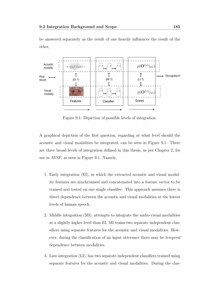
9.2 Integration Background and Scope 185
be answered separately as the result of one heavily influences the result of the
other.
Classifier
(MI ?)
Features
(EI ?)
Scores
(LI ?)Recognition?
Acoustic modality
Visual modality
Real World
PSfrag replacements
p(Oa|ωi)
p(Ov|ωi)
Figure 9.1: Depiction of possible levels of integration.
A graphical depiction of the first question, regarding at what level should the
acoustic and visual modalities be integrated, can be seen in Figure 9.1. There
are three broad levels of integration defined in this thesis, as per Chapter 2, for
use in AVSP, as seen in Figure 9.1. Namely,
1. Early integration (EI), in which the extracted acoustic and visual modal-
ity features are synchronised and concatenated into a feature vector to be
trained and tested on one single classifier. This approach assumes there is
direct dependence between the acoustic and visual modalities at the lowest
levels of human speech.
2. Middle integration (MI), attempts to integrate the audio-visual modalities
at a slightly higher level than EI. MI trains two separate independent clas-
sifiers using separate features for the acoustic and visual modalities. How-
ever, during the classification of an input utterance there may be temporal
dependence between modalities.
3. Late integration (LI), has two separate independent classifiers trained using
separate features for the acoustic and visual modalities. During the clas-
186 9.2 Integration Background and Scope
sification process there is no interaction between the modalities with only
the final classifier likelihood scores being combined.
The second question, of how best to integrate given a pre-defined level of inte-
gration, delves into practical dilemmas associated with the combination of clas-
sifiers and how different combination strategies have to be undertaken depend-
ing on the train/test mismatches occurring in either modality. Hidden Markov
model (HMM) classifiers are used for our experimental work due to their ability
to stochastically model the temporal fluctuations present in both modalities of
speech. HMMs are also able to naturally incorporate the three levels of integra-
tion EI, MI and LI.
In order to find answers to the two questions concerning audio-visual integra-
tion for a practical AVSP system one has to gain measures of performance for
two broad operational cases, taking into account the concepts of context and
train/test mismatch,
Case I: the narrow context case. This case occurs when optimal recognition per-
formance needs to be achieved on a given test set when there is no train/test
mismatch or when there is quantitative knowledge of the train/test mis-
match (i.e. classifier adaptation). This case can be thought of as the upper
limit of performance for an AVSP application as it is rare to have a priori
knowledge about the test set during recognition.
Case II: the broad context case. A specific condition of this case is that the clas-
sifier has only limited knowledge of the train/test mismatch (ie. classifier
exaptation, where there is no quantitative a priori knowledge that noise or
some other parameter in the test set has been changed except in the nature
of the scores received from the classifiers). This case can be thought of as
the lower limit of performance for an AVSP application as it gives an indi-
cation of how generalised the knowledge attained by the AVSP application
is. A natural evaluation tool for the effectiveness of a system for this case is
9.2 Integration Background and Scope 187
the ability of the AVSP application to have some benefit in combining the
audio and video speech modalities rather than relying on just one of the
modalities. This broad context case is normally evaluated across different
train/test mismatches (eg. audio noise).
Both these cases are equally important for proper evaluation of an AVSP sys-
tem. Case I is important in an application when one wants optimal performance
and benefit of an AVSP application under certain known conditions. Case II is
important in the much more common case, where operating conditions of the test
set are varied or unknown but the user still wants a high degree of recognition
performance from the system. The strict definition of some benefit in Case II
can be interpreted as the ability to out perform the catastrophic fusion boundary
for all configurable contexts lying within the broad context being evaluated (ie.
set values of audio noise or other configurable parameter in the train/test set).
In this chapter, it will be shown that in a practical scenario, when train/test
mismatches do occur in each modality, LI is superior to the MI and EI strategies.
This superior performance can be attributed to two characteristics of LI. The first
can be described in terms of classifier flexibility. Using the Viterbi algorithm [8],
it can be shown that MI’s multistream asynchronous HMMs (MAHMM) and LI’s
combined product rule HMMs are equivalent. MAHMMs naturally allow for more
flexibility as asynchronous modality state transitions are allowed where as in fully
trained EI HMMs or in MI’s multistream synchronous HMMs (MSHMM) such
transitions are not allowed. The second characteristic of benefit in the LI strategy
can be found in the assumption of train/test mismatches occurring in both audio
and video classifiers. Based on the assumption that poor performance in most
AVSP applications can be attributed to train/test mismatches it is also proposed
that the main impetus of such integration is to dampen these independent errors
rather than trying to model any bimodal speech dependencies. For the LI strategy
two different combination functions are investigated, namely the weighted prod-
uct [23] and weighted sum rules. The weighted product rule is shown to give best
188 9.3 Hidden Markov Models, Training and Integration Strategies
performance for Case I under a clean context. A hybrid approach between the
weighted product and weighted sum rules is shown to give best results for Case
II when being tested across a number of broad audio noise contexts. It must be
emphasised that the work in this chapter concerning classifier combination theory
with respect to the concept of train/test mismatches is not restricted to AVSP
and can be applied to general pattern recognition problems where independent
classifiers need to be combined.
9.3 Hidden Markov Models, Training and Inte-
gration Strategies
Hidden Markov models (HMMs) were used to model audio-visual utterances us-
ing HTK ver 2.2 [48]. The M2VTS database was employed for all experiments.
The first three shots of the M2VTS database were used to train the audio-visual
HMMs with shot four being used for testing. HMMs are excellent for mod-
elling bimodal speech as they provide a natural way to stochastically capture
the temporal fluctuations of speech in each modality and are able to naturally
incorporate the three levels of integration (ie. EI, MI and LI) mentioned earlier
into their topology. MFCC acoustic features were used to represent the audio
speech modality. WLDA with mean removal and SLDA visual features were used
to represent the visual speech modality for the tasks of speech and speaker recog-
nition respectively. LDA based visual features were chosen due to their good
recognition performance, small dimensionality and their ability to be effectively
modelled using a similar HMM topology to the audio speech modality. All HMMs
were trained with delta features using the Baum Welch algorithm via HTK [48].
Speaker recognition encapsulates two tasks namely, identification and verification.
Two models were acquired for each digit: the speaker dependent model p(O|λi),
and the background model p(O|λbck). The latter, which is common to all sub-
9.3 Hidden Markov Models, Training and Integration Strategies 189
jects, captures the variability of the uttered sound. Due to the relatively small
size of the M2VTS database and the requirement for separate speaker dependent
digit HMMs all speaker dependent HMM digit models were trained by initialis-
ing training with the previously found speaker independent or background digit
model. This approach prevented variances in each model becoming too small and
allows each model to converge to sensible values for the task of speaker recogni-
tion.
Training for the EI strategy involved the synchronisation of the acoustic and
visual features. It was noted for WLDA features that superior performance was
obtained if the WLDA visual features were interpolated to have the same sample
rate as the acoustic features after the calculation of delta features, not before.
Both acoustic and visual features were concatenated into one feature vector, which
was used to train a single joint audio-visual HMM. Via an exhaustive search an 3
state, 2 mixture HMM topology was found to give best results for the speech
recognition task for both modalities. The speaker recognition task received best
results using an 2 state, 2 mixture HMM topology for both modalities. For the
MI and LI strategies, two separate independent acoustic and visual HMMs were
trained. Again via an exhaustive search, an 3 state, 3 mixture topology was
selected for the independently trained acoustic and visual HMMs used in the
speech recognition task. The speaker recognition task obtained best results using
an 2 state, 2 mixture HMM topology for both modalities.
The EI, MI and LI integration strategies when applied to HMM classifiers can be
implemented in terms of a normal, or more correctly, single stream HMM1 [8].
Considering the general case when one wishes to classify an utterance O given
by,
O = o1, . . . ,oT (9.1)
1Unless otherwise specified, as in the case of some multistream HMMs, all HMMs trainedand used in this paper are left to right.
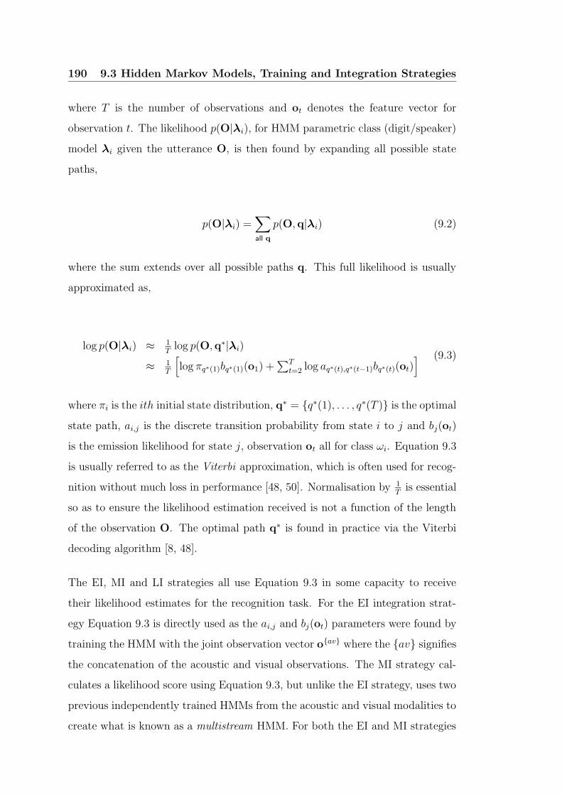
190 9.3 Hidden Markov Models, Training and Integration Strategies
where T is the number of observations and ot denotes the feature vector for
observation t. The likelihood p(O|λi), for HMM parametric class (digit/speaker)
model λi given the utterance O, is then found by expanding all possible state
paths,
p(O|λi) =∑
all q
p(O,q|λi) (9.2)
where the sum extends over all possible paths q. This full likelihood is usually
approximated as,
log p(O|λi) ≈ 1T
log p(O,q∗|λi)
≈ 1T
[
log πq∗(1)bq∗(1)(o1) +∑T
t=2 log aq∗(t),q∗(t−1)bq∗(t)(ot)] (9.3)
where πi is the ith initial state distribution, q∗ = q∗(1), . . . , q∗(T ) is the optimal
state path, ai,j is the discrete transition probability from state i to j and bj(ot)
is the emission likelihood for state j, observation ot all for class ωi. Equation 9.3
is usually referred to as the Viterbi approximation, which is often used for recog-
nition without much loss in performance [48, 50]. Normalisation by 1T
is essential
so as to ensure the likelihood estimation received is not a function of the length
of the observation O. The optimal path q∗ is found in practice via the Viterbi
decoding algorithm [8, 48].
The EI, MI and LI strategies all use Equation 9.3 in some capacity to receive
their likelihood estimates for the recognition task. For the EI integration strat-
egy Equation 9.3 is directly used as the ai,j and bj(ot) parameters were found by
training the HMM with the joint observation vector oav where the av signifies
the concatenation of the acoustic and visual observations. The MI strategy cal-
culates a likelihood score using Equation 9.3, but unlike the EI strategy, uses two
previous independently trained HMMs from the acoustic and visual modalities to
create what is known as a multistream HMM. For both the EI and MI strategies
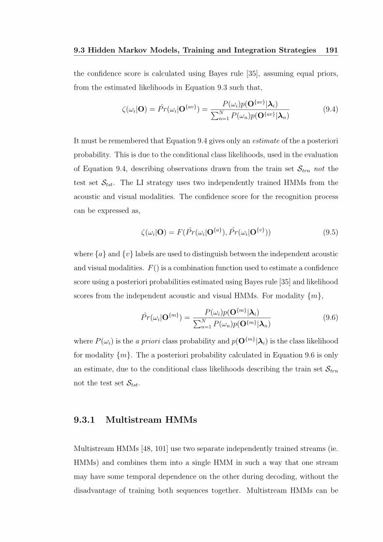
9.3 Hidden Markov Models, Training and Integration Strategies 191
the confidence score is calculated using Bayes rule [35], assuming equal priors,
from the estimated likelihoods in Equation 9.3 such that,
ζ(ωi|O) = P r(ωi|Oav) =
P (ωi)p(Oav|λi)
∑Nn=1 P (ωn)p(Oav|λn)
(9.4)
It must be remembered that Equation 9.4 gives only an estimate of the a posteriori
probability. This is due to the conditional class likelihoods, used in the evaluation
of Equation 9.4, describing observations drawn from the train set Strn not the
test set Stst. The LI strategy uses two independently trained HMMs from the
acoustic and visual modalities. The confidence score for the recognition process
can be expressed as,
ζ(ωi|O) = F (P r(ωi|Oa), P r(ωi|O
v)) (9.5)
where a and v labels are used to distinguish between the independent acoustic
and visual modalities. F () is a combination function used to estimate a confidence
score using a posteriori probabilities estimated using Bayes rule [35] and likelihood
scores from the independent acoustic and visual HMMs. For modality m,
P r(ωi|Om) =
P (ωi)p(Om|λi)
∑Nn=1 P (ωn)p(Om|λn)
(9.6)
where P (ωi) is the a priori class probability and p(Om|λi) is the class likelihood
for modality m. The a posteriori probability calculated in Equation 9.6 is only
an estimate, due to the conditional class likelihoods describing the train set Strn
not the test set Stst.
9.3.1 Multistream HMMs
Multistream HMMs [48, 101] use two separate independently trained streams (ie.
HMMs) and combines them into a single HMM in such a way that one stream
may have some temporal dependence on the other during decoding, without the
disadvantage of training both sequences together. Multistream HMMs can be
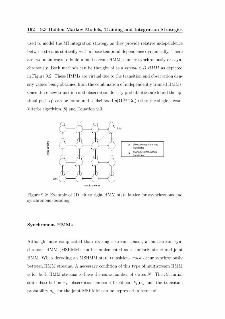
192 9.3 Hidden Markov Models, Training and Integration Strategies
used to model the MI integration strategy as they provide relative independence
between streams statically with a loose temporal dependence dynamically. There
are two main ways to build a multistream HMM, namely synchronously or asyn-
chronously. Both methods can be thought of as a virtual 2-D HMM as depicted
in Figure 9.2. These HMMs are virtual due to the transition and observation den-
sity values being obtained from the combination of independently trained HMMs.
Once these new transition and observation density probabilities are found the op-
timal path q∗ can be found and a likelihood p(Oav|λi) using the single stream
Viterbi algorithm [8] and Equation 9.3.
start
finish
(audio stream)
(vid
eo s
tream
)
allowable asynchronous transitions
allowable synchronous transitions
Figure 9.2: Example of 2D left to right HMM state lattice for asynchronous andsynchronous decoding.
Synchronous HMMs
Although more complicated than its single stream cousin, a multistream syn-
chronous HMM (MSHMM) can be implemented as a similarly structured joint
HMM. When decoding an MSHMM state transitions must occur synchronously
between HMM streams. A necessary condition of this type of multistream HMM
is for both HMM streams to have the same number of states N . The ith initial
state distribution πi, observation emission likelihood bj(ot) and the transition
probability ai,j for the joint MSHMM can be expressed in terms of,
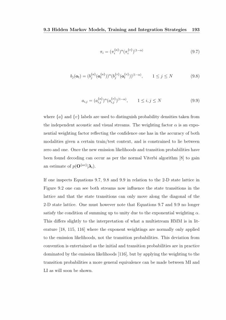
9.3 Hidden Markov Models, Training and Integration Strategies 193
πi = (πai )α(π
vi )(1−α) (9.7)
bj(ot) = (baj (o
at ))α(b
vj (o
vt ))(1−α), 1 ≤ j ≤ N (9.8)
ai,j = (aai,j )α(a
vi,j )(1−α), 1 ≤ i, j ≤ N (9.9)
where a and v labels are used to distinguish probability densities taken from
the independent acoustic and visual streams. The weighting factor α is an expo-
nential weighting factor reflecting the confidence one has in the accuracy of both
modalities given a certain train/test context, and is constrained to lie between
zero and one. Once the new emission likelihoods and transition probabilities have
been found decoding can occur as per the normal Viterbi algorithm [8] to gain
an estimate of p(Oav|λi).
If one inspects Equations 9.7, 9.8 and 9.9 in relation to the 2-D state lattice in
Figure 9.2 one can see both streams now influence the state transitions in the
lattice and that the state transitions can only move along the diagonal of the
2-D state lattice. One must however note that Equations 9.7 and 9.9 no longer
satisfy the condition of summing up to unity due to the exponential weighting α.
This differs slightly to the interpretation of what a multistream HMM is in lit-
erature [18, 115, 116] where the exponent weightings are normally only applied
to the emission likelihoods, not the transition probabilities. This deviation from
convention is entertained as the initial and transition probabilities are in practice
dominated by the emission likelihoods [116], but by applying the weighting to the
transition probabilities a more general equivalence can be made between MI and
LI as will soon be shown.
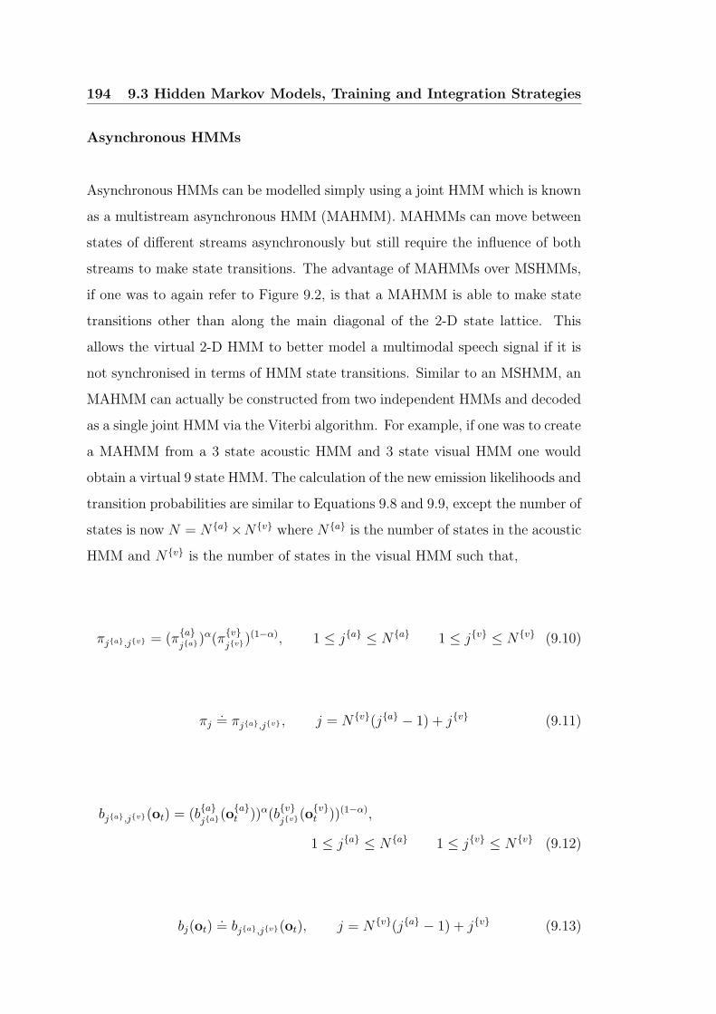
194 9.3 Hidden Markov Models, Training and Integration Strategies
Asynchronous HMMs
Asynchronous HMMs can be modelled simply using a joint HMM which is known
as a multistream asynchronous HMM (MAHMM). MAHMMs can move between
states of different streams asynchronously but still require the influence of both
streams to make state transitions. The advantage of MAHMMs over MSHMMs,
if one was to again refer to Figure 9.2, is that a MAHMM is able to make state
transitions other than along the main diagonal of the 2-D state lattice. This
allows the virtual 2-D HMM to better model a multimodal speech signal if it is
not synchronised in terms of HMM state transitions. Similar to an MSHMM, an
MAHMM can actually be constructed from two independent HMMs and decoded
as a single joint HMM via the Viterbi algorithm. For example, if one was to create
a MAHMM from a 3 state acoustic HMM and 3 state visual HMM one would
obtain a virtual 9 state HMM. The calculation of the new emission likelihoods and
transition probabilities are similar to Equations 9.8 and 9.9, except the number of
states is now N = N a×Nv where N a is the number of states in the acoustic
HMM and N v is the number of states in the visual HMM such that,
πja,jv = (πa
ja)α(π
v
jv)(1−α), 1 ≤ ja ≤ Na 1 ≤ jv ≤ Nv (9.10)
πj.= πja,jv , j = N v(ja − 1) + jv (9.11)
bja,jv(ot) = (ba
ja(oat ))α(b
v
jv(ovt ))(1−α),
1 ≤ ja ≤ Na 1 ≤ jv ≤ Nv (9.12)
bj(ot).= bja,jv(ot), j = N v(ja − 1) + jv (9.13)
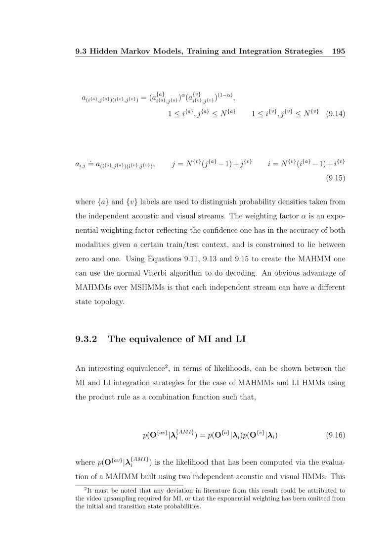
9.3 Hidden Markov Models, Training and Integration Strategies 195
a(ia,ja)(iv,jv) = (aa
ia,ja)α(a
v
iv,jv)(1−α),
1 ≤ ia, ja ≤ Na 1 ≤ iv, jv ≤ Nv (9.14)
ai,j.= a(ia,ja)(iv,jv), j = N v(ja−1)+ jv i = N v(ia−1)+ iv
(9.15)
where a and v labels are used to distinguish probability densities taken from
the independent acoustic and visual streams. The weighting factor α is an expo-
nential weighting factor reflecting the confidence one has in the accuracy of both
modalities given a certain train/test context, and is constrained to lie between
zero and one. Using Equations 9.11, 9.13 and 9.15 to create the MAHMM one
can use the normal Viterbi algorithm to do decoding. An obvious advantage of
MAHMMs over MSHMMs is that each independent stream can have a different
state topology.
9.3.2 The equivalence of MI and LI
An interesting equivalence2, in terms of likelihoods, can be shown between the
MI and LI integration strategies for the case of MAHMMs and LI HMMs using
the product rule as a combination function such that,
p(Oav|λAMIi ) = p(Oa|λi)p(O
v|λi) (9.16)
where p(Oav|λAMIi ) is the likelihood that has been computed via the evalua-
tion of a MAHMM built using two independent acoustic and visual HMMs. This
2It must be noted that any deviation in literature from this result could be attributed tothe video upsampling required for MI, or that the exponential weighting has been omitted fromthe initial and transition state probabilities.
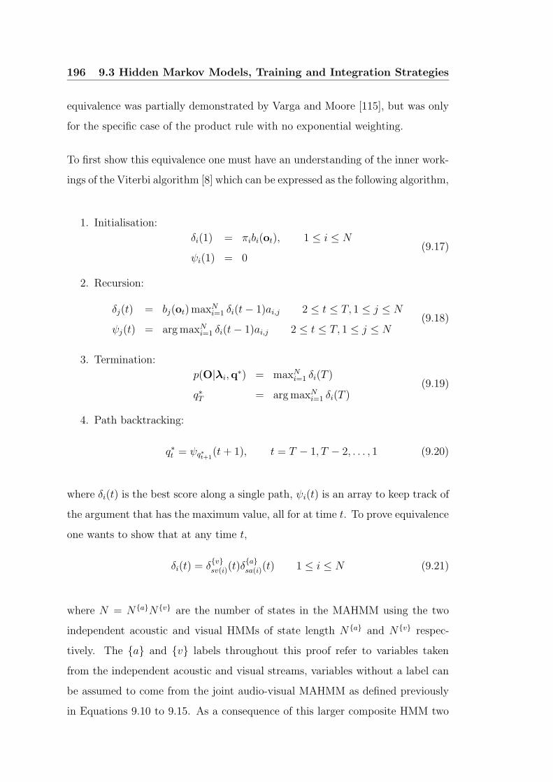
196 9.3 Hidden Markov Models, Training and Integration Strategies
equivalence was partially demonstrated by Varga and Moore [115], but was only
for the specific case of the product rule with no exponential weighting.
To first show this equivalence one must have an understanding of the inner work-
ings of the Viterbi algorithm [8] which can be expressed as the following algorithm,
1. Initialisation:
δi(1) = πibi(ot), 1 ≤ i ≤ N
ψi(1) = 0(9.17)
2. Recursion:
δj(t) = bj(ot) maxNi=1 δi(t− 1)ai,j 2 ≤ t ≤ T, 1 ≤ j ≤ N
ψj(t) = arg maxNi=1 δi(t− 1)ai,j 2 ≤ t ≤ T, 1 ≤ j ≤ N
(9.18)
3. Termination:
p(O|λi,q∗) = maxN
i=1 δi(T )
q∗T = arg maxNi=1 δi(T )
(9.19)
4. Path backtracking:
q∗t = ψq∗t+1(t+ 1), t = T − 1, T − 2, . . . , 1 (9.20)
where δi(t) is the best score along a single path, ψi(t) is an array to keep track of
the argument that has the maximum value, all for at time t. To prove equivalence
one wants to show that at any time t,
δi(t) = δvsv(i)(t)δ
asa(i)(t) 1 ≤ i ≤ N (9.21)
where N = N aNv are the number of states in the MAHMM using the two
independent acoustic and visual HMMs of state length N a and Nv respec-
tively. The a and v labels throughout this proof refer to variables taken
from the independent acoustic and visual streams, variables without a label can
be assumed to come from the joint audio-visual MAHMM as defined previously
in Equations 9.10 to 9.15. As a consequence of this larger composite HMM two

9.3 Hidden Markov Models, Training and Integration Strategies 197
look up tables ja = sa(jav) and jv = sv(ja) must be defined so as to
provide a mapping between the MAHMM and the two independent HMMs they
were created from such that,
sa(j) = ja, j = N v(ja − 1) + jv, 1 ≤ ja ≤ Na, 1 ≤ jv ≤ Nv
(9.22)
sv(j) = jv, j = N v(ja − 1) + jv, 1 ≤ ja ≤ Na, 1 ≤ jv ≤ Nv
(9.23)
The equivalence proposed in Equation 9.21 is enough to satisfy Equation 9.16
as the value δi(t), due to the nature of the Viterbi algorithm, gives the final
likelihood p(O|λi,q∗) and optimal state sequence q∗. Using Equation 9.18 from
the Viterbi algorithm one has at any time t for an MAHMM,
δj(t) = bj(ot)N
maxi=1
δi(t− 1)ai,j (9.24)
it is also known at least at t = 2 that
δi(t− 1) = δasa(i)(t− 1)δ
vsv(i)(t− 1) (9.25)
using the identity
maxx,y O(x, y) = maxx,y Ox(x) ·Oy(y)
= maxxOx(x) · maxy Oy(y)(9.26)
it can be deduced by induction for Equation 9.21 to hold for all t, equivalence
has to be demonstrated in terms of the individual acoustic and visual HMMs, as
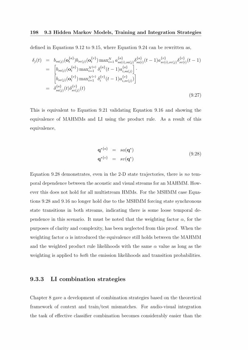
198 9.3 Hidden Markov Models, Training and Integration Strategies
defined in Equations 9.12 to 9.15, where Equation 9.24 can be rewritten as,
δj(t) = bsa(j)(oat )bsv(j)(o
vt ) maxN
i=1 aasa(i),sa(j)δ
asa(i)(t− 1)a
vsv(i),sv(j)δ
vsv(i)(t− 1)
=[
bsa(j)(oat ) maxNa
i=1 δai (t− 1)a
ai,sa(j)
]
·[
bsv(j)(ovt ) maxNv
i=1 δvi (t− 1)a
vi,sv(j))
]
= δasa(j)(t)δ
vsv(j)(t)
(9.27)
This is equivalent to Equation 9.21 validating Equation 9.16 and showing the
equivalence of MAHMMs and LI using the product rule. As a result of this
equivalence,
q∗a = sa(q∗)
q∗v = sv(q∗)(9.28)
Equation 9.28 demonstrates, even in the 2-D state trajectories, there is no tem-
poral dependence between the acoustic and visual streams for an MAHMM. How-
ever this does not hold for all multistream HMMs. For the MSHMM case Equa-
tions 9.28 and 9.16 no longer hold due to the MSHMM forcing state synchronous
state transitions in both streams, indicating there is some loose temporal de-
pendence in this scenario. It must be noted that the weighting factor α, for the
purposes of clarity and complexity, has been neglected from this proof. When the
weighting factor α is introduced the equivalence still holds between the MAHMM
and the weighted product rule likelihoods with the same α value as long as the
weighting is applied to both the emission likelihoods and transition probabilities.
9.3.3 LI combination strategies
Chapter 8 gave a development of combination strategies based on the theoretical
framework of context and train/test mismatches. For audio-visual integration
the task of effective classifier combination becomes considerably easier than the
9.3 Hidden Markov Models, Training and Integration Strategies 199
generalised task, as only two independent domains/modalitites are being dealt
with. The optimal combination scheme, assuming independence between the
acoustic and visual modalities, is the product rule,
Fpr(Pr(ωi|Oa), P r(ωi)|O
v).= Pr(ωi|O
a)Pr(ωi)|Ov)P (ωi)
−1 (9.29)
where Pr(ωi|om) are the error free a posteriori class probabilities for modal-
ity m = a or v and P (ωi) are the a priori class probabilities. In practice one
has only access to a posteriori probability estimates P r(ωi|O) = Pr(ωi|O)+εi(O)
not the true a posteriori probabilities. The confidence error εi(O) stems from
practical train/test mismatches making the combination function Fpr() in Equa-
tion 9.29, suboptimal in most practical scenarios.
These confidence errors can be dampened to some extent and improved recogni-
tion performance enjoyed through the judicious choice of combination strategies.
Two combination strategies were developed in Chapter 8 to provide such dampen-
ing, namely the weighted product and weighted sum rules. The weighted product
rule derived from the generalised form in Equation 8.6 can be defined, in terms of
estimated conditional class a posteriori probabilities stemming from the acoustic
and visual modalities, to approximate the ideal error free product rule, in terms
of the decision boundaries it realises,
Fwpr(P r(ωi|Oa), P r(ωi|O
v)) = P r(ωi|Oa)αP r(ωi|O
v)(1−α) (9.30)
Similarly, the weighted sum rule derived from the generalised form in Equa-
tion 8.24 can be defined to approximate the ideal error free product rule, in
terms of the decision boundaries it realises,
Fwsr(P r(ωi|Oa), P r(ωi|O
v)) = αPr(ωi|Oa) + (1 − α)P r(ωi|O
v) (9.31)

200 9.3 Hidden Markov Models, Training and Integration Strategies
The weighting factor α, which is constrained to lie between zero and one, is
used for both Equations 9.29 and 9.31 as an avenue for dampening the effects of
train/test mismatches.
9.3.4 Calculating a suitable α
The weighting factor α is used in both MI and LI HMM integration strategies
to provide dampening to confidence errors introduced as a result of train/test
mismatches. In Section 9.3.2 it was shown that an equivalence exists between
MI’s MAHMM and LI’s weighted product rule using two independent HMMs.
This equivalence can be used to simplify the calculation of a suitable α as one
only has to deal with the LI strategy. Admittedly MSHMMs do not have a direct
equivalence to LI, but have been shown [26] empirically, to perform well with an
optimal weighting factor α found using LI’s weighted product rule. For LI the
weighted product and weighted sum rules were investigated to derive a suitable
weighting in the presence of audio-visual train/test mismatches. The formulation
of the α weighting factor is given by,
α =βa
βa + βv
(9.32)
where the βa and βv values are used to dampen confidence error in the acoustic
and visual classifiers respectively. The βa and βv values may act in an exaptive
or adaptive capacity depending on the type of mismatch. Both βa and βv values
lie between zero and one, with a β value of one signifying there is no train/test
mismatch in that modality.
Irrespective of what capacity the α factor is acting in (i.e. adaptation or exapta-
tion) an optimal weighting factor α∗ can be found through an exhaustive search
of values between zero and one. An example of the exhaustive search process can
be seen for both the weighted product and weighted sum rules in Figure 9.3 over
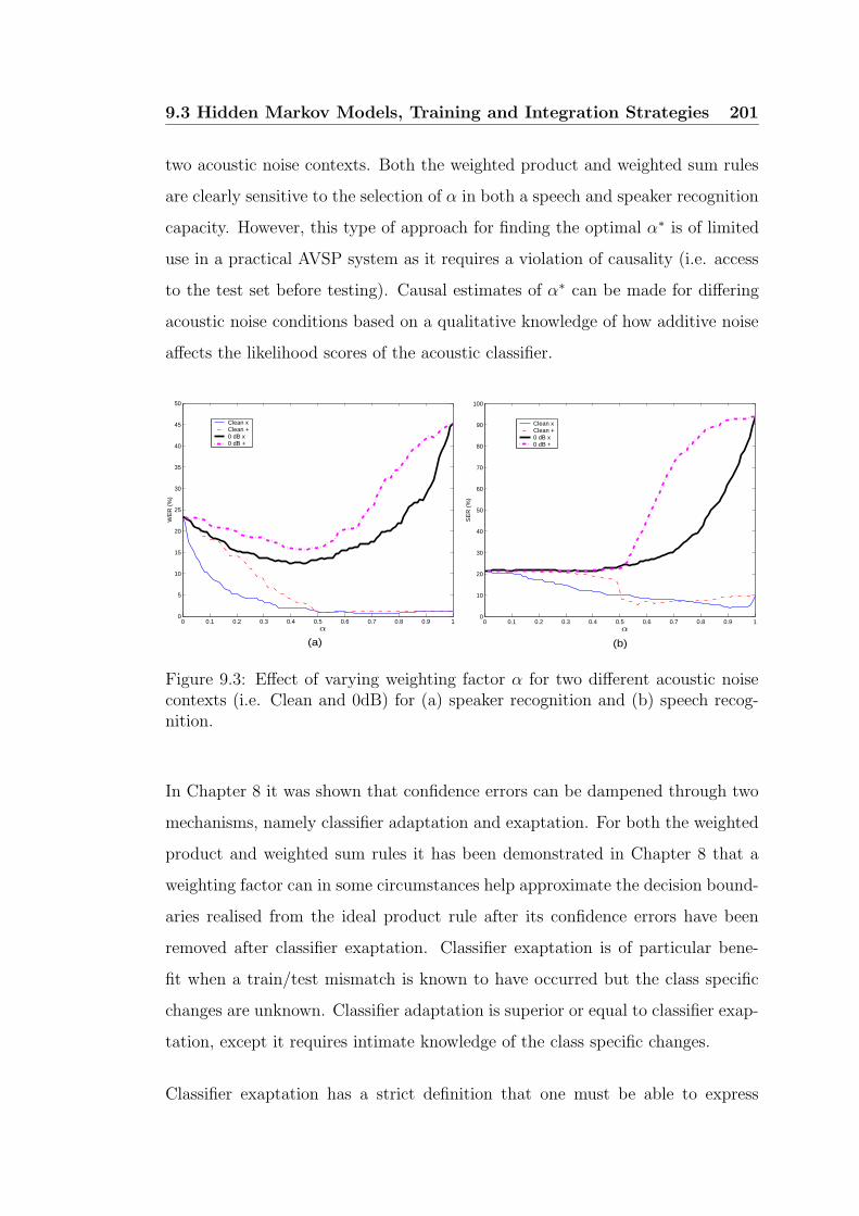
9.3 Hidden Markov Models, Training and Integration Strategies 201
two acoustic noise contexts. Both the weighted product and weighted sum rules
are clearly sensitive to the selection of α in both a speech and speaker recognition
capacity. However, this type of approach for finding the optimal α∗ is of limited
use in a practical AVSP system as it requires a violation of causality (i.e. access
to the test set before testing). Causal estimates of α∗ can be made for differing
acoustic noise conditions based on a qualitative knowledge of how additive noise
affects the likelihood scores of the acoustic classifier.
0 0.1 0.2 0.3 0.4 0.5 0.6 0.7 0.8 0.9 10
10
20
30
40
50
60
70
80
90
100
SE
R (
%)
Clean xClean +0 dB x 0 dB +
(a) (b)
0 0.1 0.2 0.3 0.4 0.5 0.6 0.7 0.8 0.9 10
5
10
15
20
25
30
35
40
45
50
WE
R (
%)
Clean xClean +0 dB x 0 dB +
PSfrag replacementsα α
Figure 9.3: Effect of varying weighting factor α for two different acoustic noisecontexts (i.e. Clean and 0dB) for (a) speaker recognition and (b) speech recog-nition.
In Chapter 8 it was shown that confidence errors can be dampened through two
mechanisms, namely classifier adaptation and exaptation. For both the weighted
product and weighted sum rules it has been demonstrated in Chapter 8 that a
weighting factor can in some circumstances help approximate the decision bound-
aries realised from the ideal product rule after its confidence errors have been
removed after classifier exaptation. Classifier exaptation is of particular bene-
fit when a train/test mismatch is known to have occurred but the class specific
changes are unknown. Classifier adaptation is superior or equal to classifier exap-
tation, except it requires intimate knowledge of the class specific changes.
Classifier exaptation has a strict definition that one must be able to express
202 9.3 Hidden Markov Models, Training and Integration Strategies
the true class likelihood p(O|ωi) as the summation of two components, namely
P (Ω)p(O|λi) and P (Ω)p(O|Ω). The first term P (Ω)p(O|λi) represents the clas-
sifier’s ability to make a decision within the known knowledge context (i.e. O ∈
Strn). The second term P (Ω)p(O|Ω) is common to all classes and represents the
classifier’s ability not to make a decision outside the known knowledge context
(i.e. O /∈ Strn). P (Ω) and P (Ω) are the priors for an observation utterance O
coming from the known and unknown context respectively.
In reality one can never have access to the true form of P (Ω)p(O|Ω) as this re-
quires a violation of causality. However, steps can be taken to dampen their effect
that do not violate causality, by defining a critical region outside of which the
effects of the mismatch likelihood p(O|Ω) become detrimental to optimal classi-
fier combination using the error free product rule3. The weighted sum rule has
been shown to be an invaluable tool in such an instance as it, in the presence
of a suitably large mismatch, approximates the optimal error free product rule.
Additionally the linear weighting factor α used in the weighted sum rule, when
equal priors are being used, has been shown empirically in Chapter 8 to provide a
mechanism for further dampening that closely approximates the decision bound-
aries realised using the error free product rule in the presence of most mismatches.
In practice it is difficult to find an optimal linear weighting factor α∗ that does
not violate causality, in causal practical situations α∗ = 0.5 is commonly used.
The weighted product rule on the other hand, has been shown theoretically and
empirically not to approximate well the decision boundaries realised by the ideal
product rule after exaptation. This is due partly to the severe nature of the prod-
uct rule in the presence of confidence errors and the inability of the weighting
factor to adequately approximate the effects of the mismatch likelihood p(O|Ω)
during exaptation. In Chapter 8 it was shown however, that for some types of
mismatch, specifically a scale mismatch, the exponential weighting factor used
in the weighted product rule acts in an adaptive not exaptive capacity. This
3The error free ideal product rule refers to the decision rules realised after exapting, notadapting, a classifier to changes in the train and test sets
9.3 Hidden Markov Models, Training and Integration Strategies 203
characteristic can find benefit in the acoustic speech modality where it has been
shown that the cepstral speech feature distribution shrinks [83] in the presence of
acoustic additive noise, whilst still partially maintaining its position and orienta-
tion. In the presence of such additive noise the weighting factor βa can adapt to
this isotropic shrinkage,
βa =σ2
trn
σ2tst
(9.33)
where σ2trn and σ2
tst are the isotropic variances of the train Strn and test Stst sets
respectively. It must be emphasised that Equation 9.33 makes the assumption
that all train/test mismatches in the acoustic modality stem solely from changes
in acoustic noise.
For most AVSP applications additive acoustic noise is the most common form
of varying train/test mismatch, making the acoustic modality’s βa dampening
value of greater significance than the visual modality’s βv dampening value, which
is normally fixed and typically acts in an exaptive not adaptive capacity. Look-
ing at Equations 9.32 and 9.33, it can be seen if the varying form of train/test
mismatch stems from acoustic noise, then the optimal weighting factor α∗ will
be proportional to βa. Dupont and Luettin [18] reported such a relationship, but
the link between cepstral shrinkage and the weighting factor α was never made.
This proportionality can be equated to Equation 9.33 as,
βa =α∗
trn
α∗tst
(9.34)
where α∗trn and α∗
tst are the optimal weighting factors for the train set and test
set conditions respectively.
Unfortunately, the ability to find the homoscedastic variance σ2tst of the test set
requires a violation of causality. From Equation 8.78 in Chapter 8 one can make
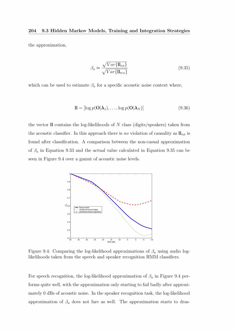
204 9.3 Hidden Markov Models, Training and Integration Strategies
the approximation,
βa ≈
√
V arlltst√
V arlltrn(9.35)
which can be used to estimate βa for a specific acoustic noise context where,
ll = [log p(O|λ1), . . . , log p(O|λN)] (9.36)
the vector ll contains the log-likelihoods of N class (digits/speakers) taken from
the acoustic classifier. In this approach there is no violation of causality as lltst is
found after classification. A comparison between the non-casual approximation
of βa in Equation 9.33 and the actual value calculated in Equation 9.35 can be
seen in Figure 9.4 over a gamut of acoustic noise levels.
−10−505101520253035400.2
0.3
0.4
0.5
0.6
0.7
0.8
0.9
1
SNR (dB)
Noise based Likelihood based (digit) Likelihood based (speaker)
PSfrag replacements
βa
Figure 9.4: Comparing the log-likelihood approximations of βa using audio log-likelihoods taken from the speech and speaker recognition HMM classifiers.
For speech recognition, the log-likelihood approximation of βa in Figure 9.4 per-
forms quite well, with the approximation only starting to fail badly after approxi-
mately 0 dBs of acoustic noise. In the speaker recognition task, the log-likelihood
approximation of βa does not fare as well. The approximation starts to dras-

9.3 Hidden Markov Models, Training and Integration Strategies 205
tically fail after only 10 dBs of acoustic noise. The poorer performance of the
acoustic speaker recognition classifier can be attributed to it being marginally
undertrained, as stated in Chapter 7, in comparison to the relatively well trained
acoustic speech recognition classifier.
It must be remembered, from Chapter 7, that the visual modality’s classifier for
both speech and speaker recognition are undertrained. If there was no train/test
mismatch in the video modality then βv = 1 could be assumed, however in the
presence of a train/test mismatch this assumption does not hold. An empirical
value for βv can be found by assuming in clean acoustic conditions that βa = 1
provided the classifier is not undertrained. Given an optimal weighting α∗cln found
under clean acoustic conditions one can then find βv as,
βv =1 − α∗
cln
α∗cln
(9.37)
For the speech and speaker recognition tasks empirically it was found βv = 0.57
and βv = 0.10 respectively. Using this estimate of βv one can gauge the effective-
ness of modelling weighting factor α∗ based on the cepstral shrinking nature of
acoustic speech in additive noise. Figure 9.5 contains (a) speech recognition and
(b) speaker recognition performance rates for calculating α∗ by an,
exhaustive search technique: where α is varied between zero and one, with
an exhaustive search conducted to find the best weighting α∗ in terms of
recognition performance.
noise based technique: where the homoscedastic variance σ2MFCC(NOISE) of
the acoustic MFCC features with deltas is used to approximate α∗. Equa-
tions 9.32 and 9.33 are used to calculate α∗, where σ2trn = σ2
MFCC(40dB)
and σ2tst = σ2
MFCC(NOISE). The notation of σ2MFCC(NOISE) refers to the
homoscedastic variance of MFCC features with a certain amount of additive
acoustic noise.
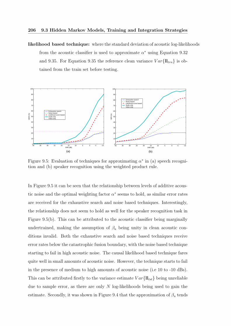
206 9.3 Hidden Markov Models, Training and Integration Strategies
likelihood based technique: where the standard deviation of acoustic log-likelihoods
from the acoustic classifier is used to approximate α∗ using Equation 9.32
and 9.35. For Equation 9.35 the reference clean variance V arlltrn is ob-
tained from the train set before testing.
10505101520253035400
10
20
30
40
50
60
70
80
90
100
SNR (dB)
SE
R (
%)
Exhaustive search Noise based Likelihood score basedAudio only Video only
(a) (b)
- - - -10505101520253035400
10
20
30
40
50
60
70
80
90
100
SNR (dB)
WE
R (
%)
Exhaustive search Noise based Likelihood score basedAudio only Video only
- -PSfrag replacements
α
Figure 9.5: Evaluation of techniques for approximating α∗ in (a) speech recogni-tion and (b) speaker recognition using the weighted product rule.
In Figure 9.5 it can be seen that the relationship between levels of additive acous-
tic noise and the optimal weighting factor α∗ seems to hold, as similar error rates
are received for the exhaustive search and noise based techniques. Interestingly,
the relationship does not seem to hold as well for the speaker recognition task in
Figure 9.5(b). This can be attributed to the acoustic classifier being marginally
undertrained, making the assumption of βa being unity in clean acoustic con-
ditions invalid. Both the exhaustive search and noise based techniques receive
error rates below the catastrophic fusion boundary, with the noise based technique
starting to fail in high acoustic noise. The causal likelihood based technique fares
quite well in small amounts of acoustic noise. However, the technique starts to fail
in the presence of medium to high amounts of acoustic noise (i.e 10 to -10 dBs).
This can be attributed firstly to the variance estimate V arlltst being unreliable
due to sample error, as there are only N log-likelihoods being used to gain the
estimate. Secondly, it was shown in Figure 9.4 that the approximation of βa tends
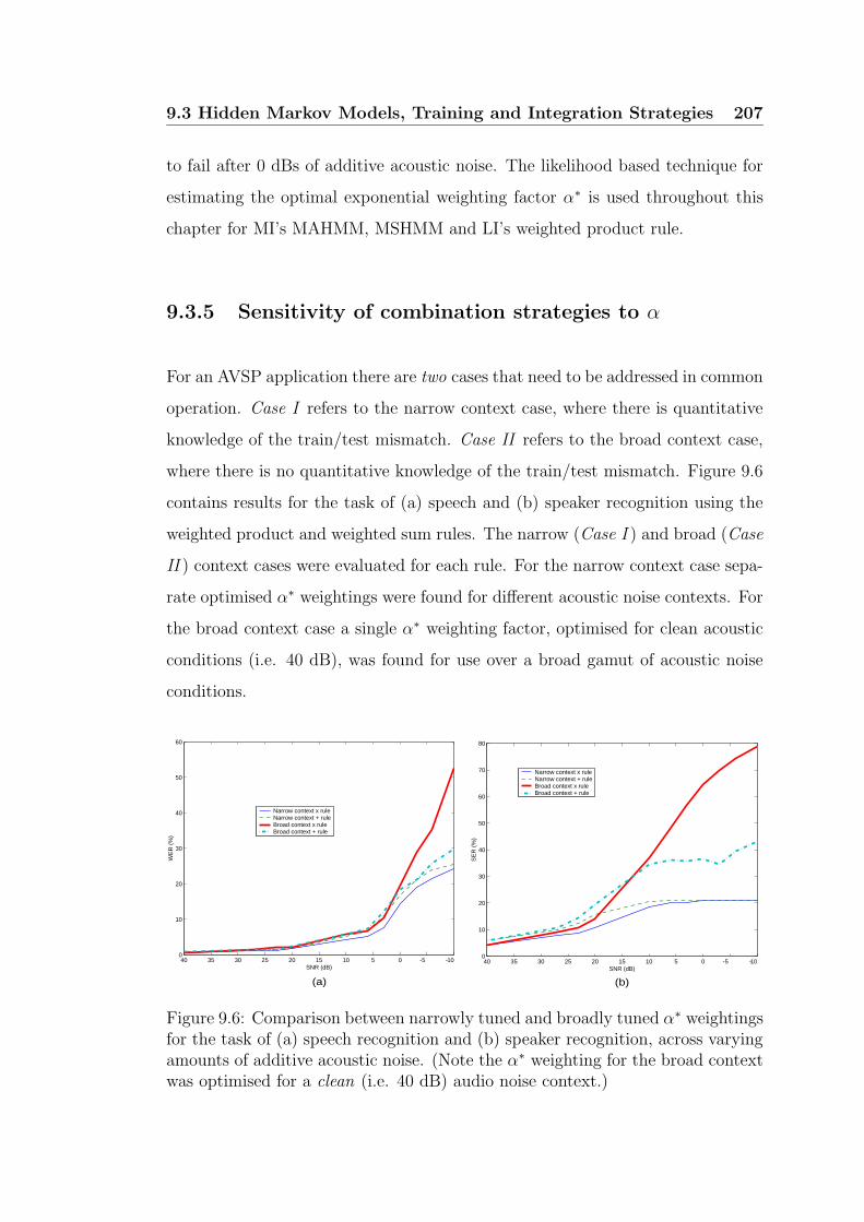
9.3 Hidden Markov Models, Training and Integration Strategies 207
to fail after 0 dBs of additive acoustic noise. The likelihood based technique for
estimating the optimal exponential weighting factor α∗ is used throughout this
chapter for MI’s MAHMM, MSHMM and LI’s weighted product rule.
9.3.5 Sensitivity of combination strategies to α
For an AVSP application there are two cases that need to be addressed in common
operation. Case I refers to the narrow context case, where there is quantitative
knowledge of the train/test mismatch. Case II refers to the broad context case,
where there is no quantitative knowledge of the train/test mismatch. Figure 9.6
contains results for the task of (a) speech and (b) speaker recognition using the
weighted product and weighted sum rules. The narrow (Case I ) and broad (Case
II ) context cases were evaluated for each rule. For the narrow context case sepa-
rate optimised α∗ weightings were found for different acoustic noise contexts. For
the broad context case a single α∗ weighting factor, optimised for clean acoustic
conditions (i.e. 40 dB), was found for use over a broad gamut of acoustic noise
conditions.
10505101520253035400
10
20
30
40
50
60
70
80
SNR (dB)
SE
R (
%)
Narrow context x ruleNarrow context + ruleBroad context x rule Broad context + rule
10505101520253035400
10
20
30
40
50
60
SNR (dB)
WE
R (
%)
Narrow context x ruleNarrow context + ruleBroad context x rule Broad context + rule
(a) (b)
- - - -
Figure 9.6: Comparison between narrowly tuned and broadly tuned α∗ weightingsfor the task of (a) speech recognition and (b) speaker recognition, across varyingamounts of additive acoustic noise. (Note the α∗ weighting for the broad contextwas optimised for a clean (i.e. 40 dB) audio noise context.)
208 9.3 Hidden Markov Models, Training and Integration Strategies
In Figure 9.6 it can be seen that the weighted product rule performs best for the
narrow context case for both the speech and speaker recognition tasks, with the
weighted sum rule also achieving good performance. Conversely, for the broad
context case, where α∗ was optimised only for clean acoustic conditions, the
weighted product rule performs badly while the weighted sum rule is considerably
less sensitive to finding the optimal weighting.
9.3.6 A hybrid between product and sum rules
Kittler [5] hypothesised that a non-linear combination rule may in fact give supe-
rior performance over the product or sum rules. In experimental work [26, 117],
a hybrid combination scheme has been devised for LI in AVSP using both the
weighted sum and weighted product rules based on a theoretical, empirical and
heuristic understanding of where they work effectively. The hybrid combination
strategy is defined as,
Fhyb(P r(ωi|Oa), P r(ωi|O
v)) =
Fwsr(P r(ωi|Oa), P r(ωi|O
v)),√
V arll < Th
Fwpr(P r(ωi|Oa), P r(ωi|O
v)),√
V arll ≥ Th(9.38)
The scheme uses the standard deviation of the of N acoustic log-likelihoods ob-
tained from a given acoustic utterance Oa to dictate when the weighted sum
or weighted product rule should be used. The decision rule in Equation 9.38 is
based purely on the acoustic log likelihoods. The threshold Th, along with the
optimised weighting factors for the weighted product rule α∗wpr and weighted sum
rule α∗wsr used in Equation 9.38 were determined empirically to optimise perfor-
mance across all acoustic noise levels. For the speech recognition task it was
empirically found Th = 3 and α∗wsr = 0.5. For the speaker recognition task it
was empirically found Th = 9 and α∗wsr = 0.5. For the weighted product rule the
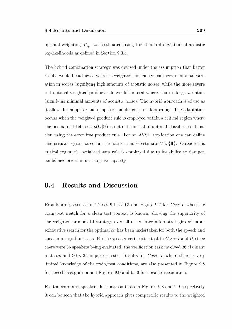
9.4 Results and Discussion 209
optimal weighting α∗wpr was estimated using the standard deviation of acoustic
log-likelihoods as defined in Section 9.3.4.
The hybrid combination strategy was devised under the assumption that better
results would be achieved with the weighted sum rule when there is minimal vari-
ation in scores (signifying high amounts of acoustic noise), while the more severe
but optimal weighted product rule would be used where there is large variation
(signifying minimal amounts of acoustic noise). The hybrid approach is of use as
it allows for adaptive and exaptive confidence error dampening. The adaptation
occurs when the weighted product rule is employed within a critical region where
the mismatch likelihood p(O|Ω) is not detrimental to optimal classifier combina-
tion using the error free product rule. For an AVSP application one can define
this critical region based on the acoustic noise estimate V arll. Outside this
critical region the weighted sum rule is employed due to its ability to dampen
confidence errors in an exaptive capacity.
9.4 Results and Discussion
Results are presented in Tables 9.1 to 9.3 and Figure 9.7 for Case I, when the
train/test match for a clean test context is known, showing the superiority of
the weighted product LI strategy over all other integration strategies when an
exhaustive search for the optimal α∗ has been undertaken for both the speech and
speaker recognition tasks. For the speaker verification task in Cases I and II, since
there were 36 speakers being evaluated, the verification task involved 36 claimant
matches and 36 × 35 impostor tests. Results for Case II, where there is very
limited knowledge of the train/test conditions, are also presented in Figure 9.8
for speech recognition and Figures 9.9 and 9.10 for speaker recognition.
For the word and speaker identification tasks in Figures 9.8 and 9.9 respectively
it can be seen that the hybrid approach gives comparable results to the weighted

210 9.4 Results and Discussion
product rule in low noise whilst receiving good results in high noise. For the
subject verification task however, the weighted sum rule received best results in
terms of equal error rate (EER) falling just below those received for the weighted
product rule in clean conditions and giving results closest to that of video only
in high noise. It must be noted that the hybrid rule used in the verification task
had its threshold for switching between product and sum rules optimised for the
identification not verification task.
Results in Table 9.1 to 9.3 for Case I showed that MI’s MSHMMs perform better
than EI’s HMMs in both the speech and speaker recognition tasks. Even though
both techniques enforce state transitions between modalities synchronously (ie.
allowing movement only along the 2-D state lattice diagonally) the MSHMMs
superior performance can be attributed to two characteristics. Firstly, since the
acoustic and visual modalities have been trained separately for MSHMMs the
resultant classifiers are much less likely to be undertrained to the same degree
as an EI HMM due to independence being assumed between modalities. Sec-
ondly, the EI implementation employed had no ability to dampen errors unlike
MSHMMs which used an weighting factor α∗ in a similar manner to its MAHMM
cousin. For Case I results it must be noted that optimal weighting factors were
found for all integration strategies through an exhaustive search. Case II results
were found using the causal likelihood based approximation of α∗ based on the
standard deviation of log-likelihood scores received from the acoustic modality’s
classifier for the weighted product rule and a static α∗ = 0.5 for the weighted
sum rule.
9.4.1 Case I
Results for Case I demonstrate the benefit of treating the acoustic and visual
modalities independently, as done in LI, in terms of classifier complexity and
its ability to dampen errors occurring in both modalities. Although receiving
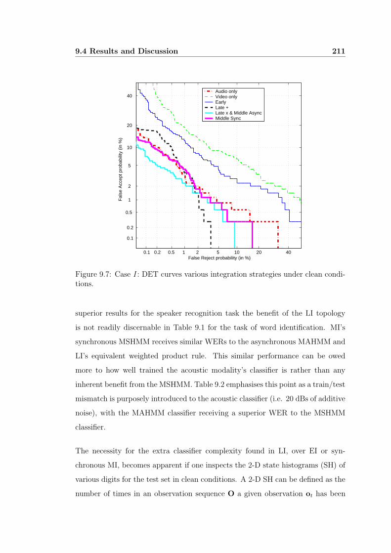
9.4 Results and Discussion 211
0.1 0.2 0.5 1 2 5 10 20 40
0.1
0.2
0.5
1
2
5
10
20
40
False Reject probability (in %)
Fal
se A
ccep
t pro
babi
lity
(in %
)
Audio only Video only Early Late + Late x & Middle AsyncMiddle Sync
Figure 9.7: Case I : DET curves various integration strategies under clean condi-tions.
superior results for the speaker recognition task the benefit of the LI topology
is not readily discernable in Table 9.1 for the task of word identification. MI’s
synchronous MSHMM receives similar WERs to the asynchronous MAHMM and
LI’s equivalent weighted product rule. This similar performance can be owed
more to how well trained the acoustic modality’s classifier is rather than any
inherent benefit from the MSHMM. Table 9.2 emphasises this point as a train/test
mismatch is purposely introduced to the acoustic classifier (i.e. 20 dBs of additive
noise), with the MAHMM classifier receiving a superior WER to the MSHMM
classifier.
The necessity for the extra classifier complexity found in LI, over EI or syn-
chronous MI, becomes apparent if one inspects the 2-D state histograms (SH) of
various digits for the test set in clean conditions. A 2-D SH can be defined as the
number of times in an observation sequence O a given observation ot has been
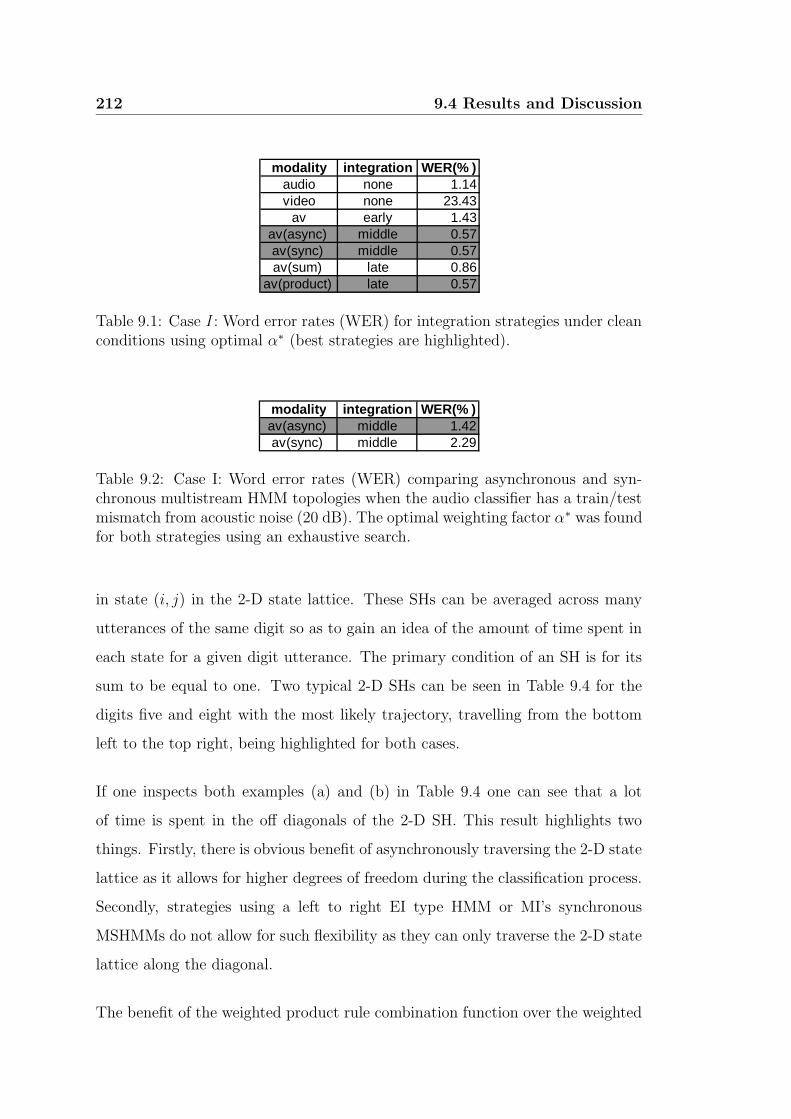
212 9.4 Results and Discussion
modality integration WER(% )audio none 1.14video none 23.43
av early 1.43av(async) middle 0.57av(sync) middle 0.57av(sum) late 0.86
av(product) late 0.57
Table 9.1: Case I : Word error rates (WER) for integration strategies under cleanconditions using optimal α∗ (best strategies are highlighted).
modality integration WER(% )av(async) middle 1.42av(sync) middle 2.29
Table 9.2: Case I: Word error rates (WER) comparing asynchronous and syn-chronous multistream HMM topologies when the audio classifier has a train/testmismatch from acoustic noise (20 dB). The optimal weighting factor α∗ was foundfor both strategies using an exhaustive search.
in state (i, j) in the 2-D state lattice. These SHs can be averaged across many
utterances of the same digit so as to gain an idea of the amount of time spent in
each state for a given digit utterance. The primary condition of an SH is for its
sum to be equal to one. Two typical 2-D SHs can be seen in Table 9.4 for the
digits five and eight with the most likely trajectory, travelling from the bottom
left to the top right, being highlighted for both cases.
If one inspects both examples (a) and (b) in Table 9.4 one can see that a lot
of time is spent in the off diagonals of the 2-D SH. This result highlights two
things. Firstly, there is obvious benefit of asynchronously traversing the 2-D state
lattice as it allows for higher degrees of freedom during the classification process.
Secondly, strategies using a left to right EI type HMM or MI’s synchronous
MSHMMs do not allow for such flexibility as they can only traverse the 2-D state
lattice along the diagonal.
The benefit of the weighted product rule combination function over the weighted
9.4 Results and Discussion 213
modality integration EER(% ) SER(% )audio none 2.00 9.71video none 7.14 21.14
av(sum) late 1.41 8.28av(product) late 1.14 4.57
av early 4.56 13.42av(async) middle 1.14 4.57av(sync) middle 2.28 8.00
Table 9.3: Case I: Equal error rates (EER) and speaker error rates (SER) forintegration strategies under clean conditions using optimal α∗ (best strategiesare highlighted for verification and identification).
Audio States1 2 3 Finish
Video 3 0.0117 0.0864 0.2325States 2 0.1624 0.1238 0.035
1 0.2897 0.0409 0.0175Start
Audio States1 2 3 Finish
Video 3 0.0125 0.0815 0.1486States 2 0.0882 0.1457 0.0853
1 0.187 0.1908 0.0604Start
(a) (b)
Table 9.4: 2-D state histograms taken from M2VTS verification set for digits (a)FIVE and (b) EIGHT.
sum rule can be understood in terms of how both rules dampen the independent
confidence errors in both modalities. The weighted product rule, has been shown
to operate in an adaptive capacity in the presence of acoustic noise. However
for Case I the acoustic conditions can be assumed to be clean. In this instance
the optimal weighting α∗ in the weighted product and weighted sum rules are
can be assumed to be acting in an exaptive capacity. The optimal weighting
factor α∗ for a given train/test mismatch can be thought of as approximating
the effects of confidence errors in an exaptive manner. This causes the weighted
product rule to act in an unstable manner as different weightings are required
for each class. The sum rule on the other hand is able to remove confidence
errors in an exaptive manner using a class independent weighting, providing equal
priors are assumed. The class dependency manifests most noticeably for LI’s
weighted product rule in the performance improvement received for the speaker
identification and verification tasks in comparison to other integration strategies.
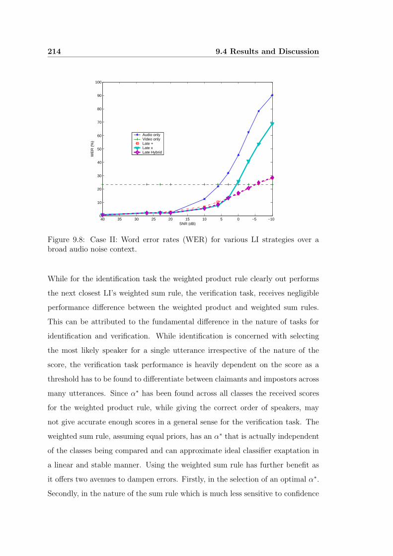
214 9.4 Results and Discussion
−10−505101520253035400
10
20
30
40
50
60
70
80
90
100
SNR (dB)
WE
R (
%)
Audio only Video only Late + Late x Late Hybrid
Figure 9.8: Case II: Word error rates (WER) for various LI strategies over abroad audio noise context.
While for the identification task the weighted product rule clearly out performs
the next closest LI’s weighted sum rule, the verification task, receives negligible
performance difference between the weighted product and weighted sum rules.
This can be attributed to the fundamental difference in the nature of tasks for
identification and verification. While identification is concerned with selecting
the most likely speaker for a single utterance irrespective of the nature of the
score, the verification task performance is heavily dependent on the score as a
threshold has to be found to differentiate between claimants and impostors across
many utterances. Since α∗ has been found across all classes the received scores
for the weighted product rule, while giving the correct order of speakers, may
not give accurate enough scores in a general sense for the verification task. The
weighted sum rule, assuming equal priors, has an α∗ that is actually independent
of the classes being compared and can approximate ideal classifier exaptation in
a linear and stable manner. Using the weighted sum rule has further benefit as
it offers two avenues to dampen errors. Firstly, in the selection of an optimal α∗.
Secondly, in the nature of the sum rule which is much less sensitive to confidence
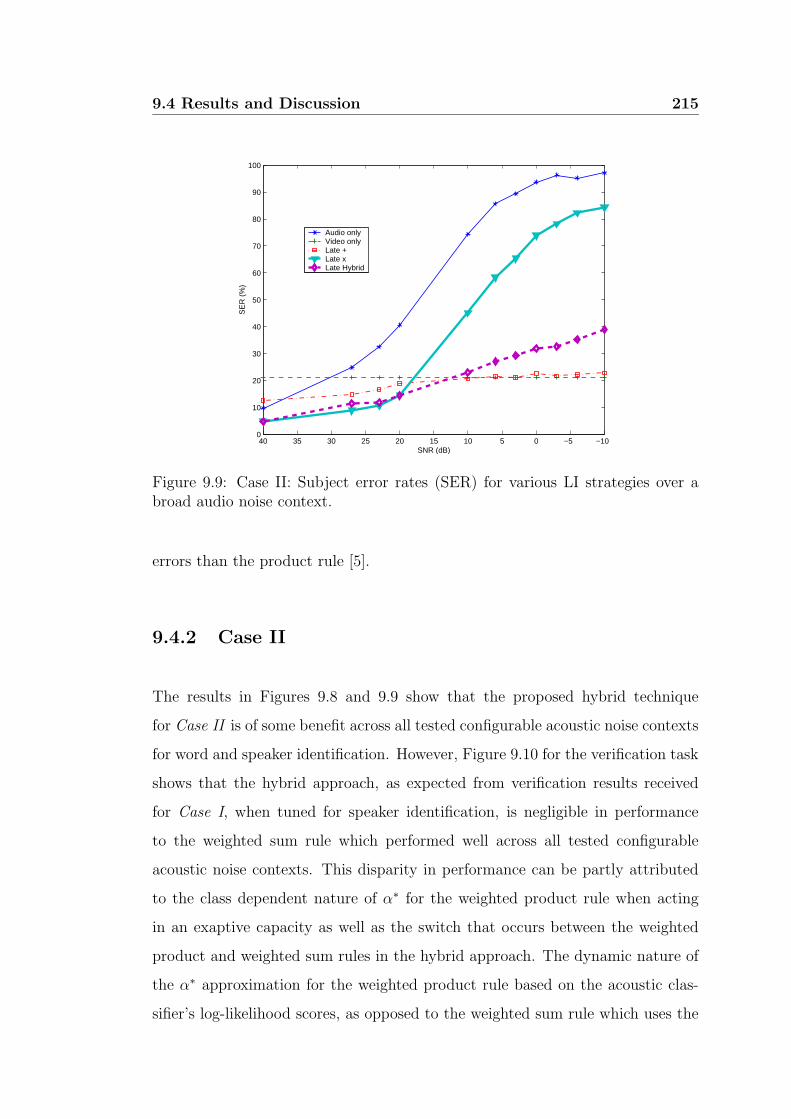
9.4 Results and Discussion 215
−10−505101520253035400
10
20
30
40
50
60
70
80
90
100
SNR (dB)
SE
R (
%)
Audio only Video only Late + Late x Late Hybrid
Figure 9.9: Case II: Subject error rates (SER) for various LI strategies over abroad audio noise context.
errors than the product rule [5].
9.4.2 Case II
The results in Figures 9.8 and 9.9 show that the proposed hybrid technique
for Case II is of some benefit across all tested configurable acoustic noise contexts
for word and speaker identification. However, Figure 9.10 for the verification task
shows that the hybrid approach, as expected from verification results received
for Case I, when tuned for speaker identification, is negligible in performance
to the weighted sum rule which performed well across all tested configurable
acoustic noise contexts. This disparity in performance can be partly attributed
to the class dependent nature of α∗ for the weighted product rule when acting
in an exaptive capacity as well as the switch that occurs between the weighted
product and weighted sum rules in the hybrid approach. The dynamic nature of
the α∗ approximation for the weighted product rule based on the acoustic clas-
sifier’s log-likelihood scores, as opposed to the weighted sum rule which uses the
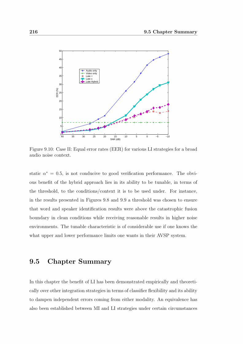
216 9.5 Chapter Summary
−10−505101520253035400
5
10
15
20
25
30
35
40
45
50
SNR (dB)
EE
R (
%)
Audio only Video only Late + Late x Late Hybrid
Figure 9.10: Case II: Equal error rates (EER) for various LI strategies for a broadaudio noise context.
static α∗ = 0.5, is not conducive to good verification performance. The obvi-
ous benefit of the hybrid approach lies in its ability to be tunable, in terms of
the threshold, to the conditions/context it is to be used under. For instance,
in the results presented in Figures 9.8 and 9.9 a threshold was chosen to ensure
that word and speaker identification results were above the catastrophic fusion
boundary in clean conditions while receiving reasonable results in higher noise
environments. The tunable characteristic is of considerable use if one knows the
what upper and lower performance limits one wants in their AVSP system.
9.5 Chapter Summary
In this chapter the benefit of LI has been demonstrated empirically and theoreti-
cally over other integration strategies in terms of classifier flexibility and its ability
to dampen independent errors coming from either modality. An equivalence has
also been established between MI and LI strategies under certain circumstances
9.5 Chapter Summary 217
in terms of a HMM classifier framework. The weighted product rule has been
shown to perform best for Case I mode of AVSP operation. The benefits of a
hybrid combination scheme have been highlighted for addressing Case II mode
of AVSP operation. Finally, a framework has been devised for dealing with the
natural train/test mismatches that occur when classifiers are used practically via
the concept of context based knowledge.
The link between cepstral shrinkage and the weighted product rule has also been
established. The benefit of gaining a measure of this shrinkage, in a causal man-
ner, from acoustic log-likelihood scores has been demonstrated. This approach
has shown to be of benefit in minimum to medium amounts of additive acous-
tic noise. Finally, a framework of classifier adaptation and exaptation has been
implemented into a practical AVSP system. The success of the hybrid combina-
tion illustrate the benefits of both the adaptation and exaptation paradigms to
addressing confidence errors stemming from train/test mismatches.


Chapter 10
Conclusions and Future Work
This chapter contains a summary of the work presented in each chapter. Addi-
tionally, conclusions and possible avenues for future work are identified.
10.1 Conclusions
In this thesis approaches in AVSP were reviewed and developed pertinent to
the tasks of speech and speaker recognition. The work conducted was primarily
focussed on addressing two points of interest in AVSP.
1. Gaining of an appropriate representation of the visual speech modality.
2. The effective integration of the acoustic and visual speech modalities in the
presence of a variety of degradations.
Work has been performed to try and address these still largely unsolved prob-
lems in AVSP. Overall the integration of the acoustic and visual modalities gave
improved and robust performance over either modality individually.
220 10.1 Conclusions
The conclusions drawn from each chapter are:
Chapter 2 gives an overview of current work in AVSP. This chapter sets up
the framework and scope of the research contained in this thesis. Specifi-
cally, insights are gained into the mechanics of speech, phonetics and the
complementary nature of speech as highlighted through the McGurk effect.
Chapter 3 delved into classifier theory identifying practical limitations asso-
ciated with the design and implementation of classifiers. Non-parametric,
discriminant and parametric classifiers were evaluated with parametric clas-
sifiers being chosen for primary usage throughout the thesis due to their
robustness and rigorous mathematical development. GMM and HMM clas-
sifier theory was intimately developed.
Chapter 4 formed a framework for the front-end of the AVSP system, con-
cerned primarily with the detection and normalisation of facial features.
The scope of the facial feature detection problem was constrained for sce-
narios common to AVSP (i.e. single subject, frontal pose, minimal head
rotation, etc.). Within this framework the benefit of finding a skin map,
through chromatic segmentation, is demonstrated as a useful technique for
constraining the search space for facial features.
Chapter 5 saw the evaluation of the appearance based object detection paradigm.
This approach gained excellent results for the tasks of eye and mouth de-
tection using a novel two class (object and background) detection model
derived in discriminant space. This discriminant space was constructed
through intra-class clustering and linear discriminant analysis (LDA).
Chapter 6 was the focus of lip location/tracking through the feature invariant
object detection paradigm. This approach used a chromatic segmentation
approach, to first successfully separate lip pixels from their primarily skin
background. This approach worked off the general premise that lip pixels
are generally redder than the paler skin pixels they coexist with. A novel
10.1 Conclusions 221
approach for fitting the labial contour, to the segmented lip image, was also
presented using gradient vector flow (GVF) fields and point distribution
models (PDM). This technique was able to fit labial shape models to many
poorly segmented lip images with good results. Chromatic distinction be-
tween the lips and skin proved to be a major stumbling block, with some
subjects having very poor chromatic distinction. This result goes against
the heuristic assumption that the lips and skin can be successfully sepa-
rated based purely on their chromaticity. As a result lip location/tracking,
based on chromatic segmentation, was not used in subsequent AVSP visual
feature extraction.
Chapter 7 was concerned with the extraction of features useful to the acoustic
and visual speech modalities for speech and speaker recognition. Tradi-
tional Mel-Frequency cepstral coefficients (MFCCs) were found to be of use
in acoustic speech and speaker recognition. In the visual modality area fea-
tures, based purely on the pixel based representation of the mouth, proved
superior to contour features, in terms of generation and robustness to noise.
A number of area features were evaluated for the tasks of speech reading
and visual speaker recognition with data driven, discriminant transforms
performing well. Mean subtraction on visual area features, for the task of
speech reading, removed unwanted variations stemming from changes in a
subject’s appearance. Additionally, there was some indication, for the task
of speech reading, that standard HMMs do not model the dynamic nature
of the visual speech modality effectively.
Chapter 8 presented a theoretical framework for effectively combining indepen-
dent classifiers. Working from the premise that classifier confidence er-
rors stem from train/test mismatches, two mechanisms can be employed
to dampen the effects of these errors namely, adaptation and exaptation.
Under matched conditions the product rule is known to be optimal for inde-
pendent classifier combination. Using the concepts of classifier adaptation
and exaptation, a number of combination strategies are developed that can
222 10.2 Future Work
dampen the effects of confidence errors without violating causality. A ben-
eficial link between acoustic feature cepstral shrinkage in the presence of
acoustic noise and the weighted product is also established.
Chapter 9 evaluates a number of integration strategies using an HMM classi-
fier. In this work it is shown that late integration (LI) strategy outperforms
middle integration (MI) and early integration (EI) for the tasks of isolated
word speech and speaker recognition. An equivalence between LI’s weighted
product rule and MI’s multistream asynchronous HMM for the case of
Viterbi decoding is shown. The superiority of LI is postulated to stem
from its ability to dampen the indepenent errors in either modality rather
than model any dependencies existing between modalities. Two broad op-
erational cases were defined for use in AVSP namely, narrow context (Case
I ) which assumes matched train/test conditions and broad context (Case
II ) in which the train/test conditions may vary. For Case I the weighted
product rule proved superior for speech and speaker recognition. In Case II
a novel hybrid approach based on the adaptive combination of the weighted
product and weighted sum rules performed best in both speech and speaker
recognition.
10.2 Future Work
A number of avenues for future work have been identified during the completion
of this thesis. These are summarised below:
(i) In Chapter 5 a novel technique using a discriminant representation of the
object and background was presented based on the appearance based ob-
ject detection paradigm. This approach used the highly effective GMM
classifier in the detection procedure. Discriminant classifiers like artificial
neural networks (ANNs) or support vector machines (SVMs) may give im-

10.2 Future Work 223
proved performance, due to their natural affinity for such static well defined
problems.
(ii) The generation of the discriminant space in Chapter 5 uses intra-class clus-
tering based on knowledge of how LDA derives a discriminant space. Fur-
ther improvement could be attained if the clustering is performed in a man-
ner that ensures each cluster has the same between-scatter matrix.
(iii) Chapter 6 highlighted some of the short comings of lip location/tracking
through chrominance for some speakers. Although not a satisfactory solu-
tion to the mouth location/tracking problem by itself, colour in many cir-
cumstances can act as an additional feature for improving location/tracking
performance. A future approach could be to somehow fuse the appearance
based and feature invariant object detection paradigms for improved facial
feature detection performance.
(iv) Additional research is required into alternate classifier designs for modelling
the temporal nature of visual speech. As indicated in Chapter 7, there is
some indication that the quasi-stationary assumptions made in standard
HMM theory may not model the visual speech modality satisfactorily.
(v) Superior visual feature extraction approaches are required for improved
visual speech and speaker recognition performance. Unlike the acoustic
modality, classifiers from Chapter 7 in the visual modality are still largely
undertrained. This indicates that current visual speech representations
are not capturing information pertinent to speech recognition and speaker
recognition and are still affected by unwanted variations.
(vi) The insights gained in independent classifier combination theory in Chap-
ter 8 could to be applied to other applications in pattern recognition where
there is a requirement for the combination of classifier confidence scores
from independent observation domains.
(vii) The novel concept of classifier exaptation, developed in Chapter 8, could

224 10.2 Future Work
readily be applied to secondary or post-classification. In this approach the
likelihood scores from a primary classifier are used to train a secondary
classifier, via a validation set, to try and gain a measure of train/test mis-
match. Using the framework of classifier exaptation, the likelihood from
such a secondary classifier could naturally be incorporated as a mismatch
likelihood p(o|Ω) for improved classifier combination performance.
(viii) The use of 2-D state histograms, presented in Chapter 9, could be used as a
possible avenue for further recognition performance in an AVSP application.
(ix) The development of a soft transition between the weighted product and
weighted sum rules could be investigated, for the hybrid combination scheme
presented in Chapter 9, rather than the hard transition implementation cur-
rently in use.
(x) The effects of visual degradations, not just acoustic, requires more study to
ensure the creation of robust AVSP systems.
Bibliography
[1] L. Rabiner and B. Juang, Fundamentals of Speech Recognition. Englewood
Cliffs, NJ: Prentice Hall, Inc., 1993.
[2] S. Pigeon, “The M2VTS database,” (Laboratoire de Telecommunications et
Teledection, Place du Levant, 2-B-1348 Louvain-La-Neuve, Belgium), 1996.
[3] P. Jourlin, J. Luettin, D. Genoud, and H. Wassner, “Acoustic-labial speaker
verification,” Pattern Recognition Letters, 1997.
[4] T. Wark, Multi-modal Speech Processing for Automatic Speaker Recogni-
tion. PhD thesis, Electrical and Electronic Systems Engineering, Queens-
land Univeristy of Technology, October 2000.
[5] J. Kittler, M. Hatef, R. Duin, and J. Matas, “On combining classifiers,”
IEEE Transacations on Pattern Analysis and Machine Intelligence, vol. 20,
pp. 226–239, March 1998.
[6] T. Chen and R. Rao, “Audio-visual integration in multimodal communica-
tion,” Proceedings of the IEEE, vol. 86, pp. 837–852, May 1998.
[7] H. McGurk and J. MacDonald, “Hearing lips and seeing voices,” Nature,
pp. 746–748, December 1976.
[8] L. R. Rabiner, “A tutorial on hidden markov models and selected applica-
tions in speech recognition,” Proceedings of the IEEE, vol. 77, pp. 257–286,
February 1989.
226 BIBLIOGRAPHY
[9] A. J. Goldschen, Continuous automatic speech recognition by lipreading.
PhD thesis, George Washington University, Washington DC, September
1993.
[10] B. Dodd and R. Campbell, eds., Hearing by Eye: The Psychology of
Lipreading. London, England: Lawrence Erlbaum Associates Ltd., 1987.
[11] D. Burnham and B. Dodd, “The McGurk effect in infants across differ-
ent languages,” in Speechreading by Humans and Machines (D. Stork and
M. Hennecke, eds.), pp. 103–114, Springer-Verlag, 1996.
[12] F. Lavagetto, “Converting speech into lip movements: A multimedia tele-
phone for hard hearing people,” IEEE Transactions on Rehabilitation En-
gineering, vol. 3, pp. 90–102, March 1995.
[13] B. Dodd, “The acquisition of lipreading skills by normally hearing chil-
dren,” in Hearing by Eye: The Psychology of Lipreading (B. Dodd and
R. Campbell, eds.), pp. 163–175, Lawrence Erlbaum Associates Ltd., 1987.
[14] A. E. Mills, “The development of phonology in blind children,” in Hearing
by Eye: The Psychology of Lipreading (B. Dodd and R. Campbell, eds.),
pp. 145–161, Lawrence Erlbaum Associates Ltd., 1987.
[15] H. W. Frowein, G. F. Smoorenburg, L. Pyters, and D. Schinkel, “Improved
speech recognition through videotelephony: Experiments with the hard
of hearing,” IEEE Journal of Selected Areas in Communications, vol. 9,
pp. 611–616, May 1991.
[16] W. Sumby and I. Pollak, “Visual contributions to speech intelligibility in
noise,” Journal of the Acoustic Society of America, vol. 26, pp. 212–215,
March 1954.
[17] C. C. Chibelushi, F. Deravi, and J. S. D. Mason, “A review of speech-based
bimodal recognition,” IEEE Transactions on Multimedia, vol. 4, pp. 23–37,
March 2000.
BIBLIOGRAPHY 227
[18] S. Dupont and J. Luettin, “Audio-visual speech modeling for continuous
speech recognition,” IEEE Transactions on Multimedia, vol. 2, pp. 141–
151, September 2000.
[19] A. Adjoudani and C. Benoit, “Audio-visual speech recognition compared
across two architectures,” in Eurospeech’95, (Madrid Spain), pp. 1563–1566,
September 1995.
[20] I. Matthews, T. Cootes, S. Cox, R. Harvey, and J. A. Bangham, “Lipread-
ing using shape, shading and scale,” in Auditory-Visual Speech Processing,
(Sydney, Australia), pp. 73–78, 1998.
[21] C. C. Chibelushi, J. S. Mason, and F. Deravi, “Integration of acoustic and
visual speech for speaker recognition,” in Eurospeech’93, (Berlin), pp. 157–
160, September 1993.
[22] M. McGrath and Q. Summerfield, “Intermodal timing relations and audio-
visual speech recognition,” Journal of the Acoustical Society of America,
vol. 77, pp. 678–685, February 1985.
[23] S. Cox, I. Matthews, and J. A. Bangham, “Combining noise compensation
with visual Information in speech recognition,” in Auditory-Visual Speech
Processing, (Rhodes), 1997.
[24] J. Luettin, G. Potamianos, and C. Neti, “Asynchronous stream modeling
for large vocabulary audio-visual speech recognition,” in International Con-
ference on Acoustics, Speech and Signal Processing, vol. 1, (Salt Lake City),
pp. 169 –172, May 2001.
[25] T. Chen, “Audiovisual speech processing,” IEEE Signal Processing Maga-
zine, vol. 18, pp. 9–21, January 2001.
[26] S. Lucey, T. Chen, S. Sridharan, and V. Chandran, “Integration strate-
gies for audio-visual speech processing: Applied to text dependent speaker
identification/verification,” IEEE Transactions on Multimedia, 2002. sub-
mitted.
228 BIBLIOGRAPHY
[27] T. Wark, Multi-modal speech processing for automatic speaker recognition.
PhD thesis, Electrical and Electronic Systems Engineering, Queensland
Univeristy of Technology, October 2000.
[28] G. Potamianos, J. Luettin, and C. Neti, “Hierarchical discriminant features
for audio-visual LVCSR,” in International Conference on Acoustics, Speech
and Signal Processing, vol. 1, pp. 165–168, 2001.
[29] J. Luettin, N. A. Thacker, and S. W. Beet, “Speaker identification by
lipreading,” in International Conference on Spoken Language Processing,
vol. 1, pp. 62–65, 1996.
[30] G. Potamianos, H. P. Graf, and E. Cosatto, “An image transform approach
for HMM based automatic lipreading,” in International Conference on Im-
age Processing, vol. 3, pp. 173–177, 1998.
[31] K. Otani and T. Hasegawa, “The image input microphone: A new nona-
coustic speech communication system by media conversion from oral mo-
tion images to speech,” IEEE Journal on Selected Areas in Communication,
vol. 13, pp. 42–48, January 1995.
[32] L. Girin, G. Feng, and J. Schwartz, “Noisy speech enhancement with fil-
ters estimated from the speaker’s lips,” in Eurospeech’95, (Madrid, Spain),
pp. 1559–1562, 1995.
[33] E. Foucher, L. Girin, and G. Feng, “Audio-visual speech coder: Using vector
quantization to exploit the audio/video correlation,” in Auditory-Visual
Speech Processing, 1998.
[34] L. Girin, L. Varin, G. Feng, and J. Schwartz, “Audiovisual speech enhance-
ment: New advances using multi-layer perceptrons,” in IEEE Second Work-
shop on Multimedia Signal Processing (P. Wong, A. Alwan, A. Ortega,
C. Kuo, and C. Nikian, eds.), pp. 77–82, December 1998.
[35] K. Fukunaga, Introduction to Statistical Pattern Recognition. 24-28 Oval
Road, London NW1 7DX: Academic Press Inc., 2nd ed., 1990.
BIBLIOGRAPHY 229
[36] J. Ghosh and K. Tumer, “Structural adaption and generalization in super-
vised feedforward networks,” Journal of Artificial Neural Networks, vol. 1,
no. 4, pp. 431–458, 1994.
[37] R. O. Duda, P. E. Hart, and D. G. Stork, Pattern Classification. New York,
NY, USA: John Wiley and Sons, Inc., 2nd ed., 2001.
[38] M. Turk and A. Pentland, “Eigenfaces for recognition,” Journal of Cognitive
Neuroscience, vol. 3, no. 1, 1991.
[39] B. Moghaddam and A. Pentland, “Probabilistic visual learning for object
representation,” IEEE Transactions on Pattern Analysis and Machine In-
telligence, vol. 19, pp. 696–710, July 1997.
[40] W. S. Sarle, “Measurement theory: Frequently asked questions,” in Dissem-
inations of the International Statistical Applications Institute, pp. 61–66,
Wichita: AGP Press, 4th ed., 1996.
[41] H. Rowley, S. Baluja, and T. Kanade, “Neural network-based face detec-
tion,” in Conference on Computer Vision and Pattern Recognition, pp. 203–
208, 1996.
[42] H. Rowely, S. Bajula, and T. Kanade, “Neural network-based face detec-
tion,” IEEE Transactions on Pattern Analysis and Machine Intelligence,
vol. 20, pp. 23–38, January 1998.
[43] C. J. C. Burges, “A tutorial on support vector machines for pattern recog-
nition,” Data Mining and Knowledge Discovery, vol. 2, no. 2, pp. 121–167,
1998.
[44] S. G. Y. Li, J. Sherrah, and H. Liddell, “Multi-view face detection using
support vector machines and eigenspace modelling,” in Fourth International
Conference on Knowledge-Based Intelligent Engineering Systems and Allied
Technologies, (Brighton, UK), pp. 241–244, August 2001.
230 BIBLIOGRAPHY
[45] D. A. Reynolds, “Experimental evaluation of features for robust speaker
identification,” IEEE Transactions on Speech and Audio Processing, vol. 2,
pp. 539–643, October 1994.
[46] A. Dempster, N. Laird, and D. Rubin, “Maximum likelihood from incom-
plete data via the EM algorithm,” Royal Statistical Society, vol. 39, pp. 1–
38, 1977.
[47] E. Kreyszig, Advanced engineering mathematics. John Wiley and Sons,
Inc., 7th ed., 1993.
[48] S. Young, D. Kershaw, J. Odell, D. Ollason, V. Valtchev, and P. Woodland,
The HTK Book (for HTK version 2.2). Entropic Ltd., 1999.
[49] A. Gersho and R. Gray, Vector Quantization and Signal Compression. 3300
AH Dordrecht, THE NETHERLANDS: Kluwer Academic Publishers, 1992.
[50] H. Bourlard and N. Morgan, “Hybrid HMM/ANN systems for speech recog-
nition: Overview and new research directions,” in Summer School on Neural
Networks, pp. 389–417, 1997.
[51] M. Yang, D. J. Kriegman, and N. Ahuja, “Detecting faces in images: A sur-
vey,” IEEE Transacations on Pattern Analysis and Machine Intelligence,
vol. 24, pp. 1–25, January 2002.
[52] O. Jesorsky, K. Kirchberg, and R. Frischholz, “Robust face detection using
the hausdorff distance,” in Third International Conference on Audio and
Video based Biometric Person Authentication, (Halmstad, Sweden), pp. 90–
95, June 2001.
[53] M. F. Augusteijn and T. L. Skujca, “Identification of human faces through
texture-based feature recognition and neural network technology,” in IEEE
Conference on Neural Networks, pp. 392–398, 1993.
[54] J. Yang and A. Waibel, “A real-time face tracker,” in Third IEEE on Appli-
cations of Computer Vision, (Sarasota, Florida, USA), pp. 142–147, 1996.
BIBLIOGRAPHY 231
[55] M. H. Yang and N. Ahuja, “Detecting human faces in color images,” in
International Conference on Image Processing, vol. 1, pp. 127–130, 1998.
[56] A. Yuille, P. W. Hallinan, and D. S. Cohen, “Feature extraction from faces
using deformable templates,” International Journal of Computer Vision,
vol. 8, no. 2, pp. 99–111, 1992.
[57] G. Chiou and J. Hwang, “Lipreading from color video,” IEEE Transactions
on Image Processing, vol. 6, pp. 1192–1195, August 1997.
[58] M. U. Ramos Sanchez, J. Matas, and J. Kittler, “Statistical chromatic-
ity models for lip tracking with B-splines,” in International Conference on
Audio and Video based Biometric Person Authentication, (Crans Montana,
Switzerland), pp. 69–76, 1997.
[59] T. F. Cootes, A. Hill, C. J. Taylor, and J. Haslam, “Use of active shape
models for locating structures in medical images,” Image and Vision Com-
puting, vol. 12, pp. 355–365, July/August 1994.
[60] T. F. Cootes, G. J. Edwards, and C. J. Taylor, “Active appearance models,”
in European Conference on Computer Vision, vol. 2, pp. 484–498, 1998.
[61] M. Yang, N. Abuja, and D. Kriegman, “Mixtures of linear subspaces for
face detection,” in Fourth IEEE International Conference on Automatic
Face and Gesture Recognition, pp. 70–76, 2000.
[62] Y. Tian, T. Kanade, and J.Cohn, “Robust lip tracking by combining shape
color and motion,” in Asian Conference on Computer Vision, pp. 1040–
1045, 2000.
[63] M. Lievin and F. Luthon, “Unsupervised lip segmentation under natural
conditions,” in International Conference on Acoustics, Speech and Signal
Processing, (Phoenix, Arizona), pp. 3065–3068, March 1999.
232 BIBLIOGRAPHY
[64] M. T. Chan, Y. Zhang, and T. S. Huang, “Real-time lip tracking and bi-
modal continuous speech recognition,” in IEEE Second Workshop on Mul-
timedia Signal Processing, pp. 65–70, 1998.
[65] R. Rao and R. M. Mersereau, “Lip modeling for visual speech recognition,”
in Twenty-Eighth Asilomar Conference on Signals, Systems and Computers,
vol. 1, pp. 587–590, 1994.
[66] J. Luettin, N. A. Thacker, and S. W. Beet, “Speechreading using shape and
intensity information,” in International Conference on Spoken Language
Processing, vol. 1, pp. 58–61, 1996.
[67] P. N. Belhumeur, J. P. Hespanha, and D. J. Kriegman, “Eigenfaces vs.
fisherfaces: Recognition using class specific linear projection,” IEEE Tran-
scations on Pattern Analysis and Machine Intelligence, vol. 19, pp. 711–720,
July 1997.
[68] S. Roweis, “EM algorithms for PCA and SPCA,” in Neural Information
Processing Systems (NIPS’97), vol. 10, pp. 626–632, 1997.
[69] M. E. Tipping and C. M. Bishop, “Probabilistic principal component analy-
sis,” Tech. Rep. NCRG/97/010, Neural Computing Research Group, Aston
University, September 1997.
[70] B. Chalmond and S. C. Girard, “Nonlinear modeling of scattered multi-
variate data and its application to shape change,” IEEE Transactions on
Pattern Analysis and Machine Intelligence, vol. 21, pp. 422–432, May 1999.
[71] D. J. Bartholomew, Latent Variable Models and Factor Analysis. London:
Griffin and Co. Ltd., 1987.
[72] H. Anton and C. Rorres, Elementary Linear Algebra. New York: John
Wiley and Sons, Inc., 7th ed., 1994.
[73] A. Martin, G. Doddington, T. Kamm, M. Ordowski, and P. Przybocki,
BIBLIOGRAPHY 233
“The DET curve in assessment of detection task performance,” in Eu-
rospeech’97, vol. 4, pp. 1895–1898, 1997.
[74] T. Wark and S. Sridharan, “An approach to statistical lip modelling for
speaker identification via chromatic feature extraction,” in International
Conference on Pattern Recognition, vol. 1, pp. 123–125, 1998.
[75] P. Delmas, P. Y. Coulon, and V. Fristot, “Automatic snakes for robust lip
boundaries extraction,” in International Conference on Acoustics, Speech
and Signal Processing, vol. 6, pp. 3069–3072, 1999.
[76] M. Kass, A. Witkins, and D. Terzopoulos, “Snakes: Active contour models,”
International Journal of Computer Vision, vol. 1, no. 4, pp. 321–331, 1987.
[77] C. Xu and J. L. Prince, “Snakes, shapes and gradient vector flow,” IEEE
Transactions on Image Processing, vol. 7, pp. 359–369, March 1998.
[78] P. E. Papamichalis, Practical Approaches to Speech Coding. Englewood
Cliffs, New Jersey: Prentice Hall Inc., 1987.
[79] S. Davis and P. Mermelstein, “Comparison of parametric representations
for monosyllabic word recognition in continuously spoken sentences,” IEEE
Transactions on Acoustics, Speech and Signal Processing, vol. 28, pp. 357–
366, August 1980.
[80] B. Gold and N. Morgan, Speech and audio signal processing: Processing
and perception of speech and music. New York: John Wiley and Sons, Inc.,
2000.
[81] E. C. Ifeachor and B. W. Jervis, Digital Signal Processing: A Practical
Approach. Wokingham, England: Addison-Wesley Publishers Company
Inc., 1993.
[82] G. Fant, Acoustic Theory of Speech Production. Gravenhage, Netherlands:
Mouton and Co., 1960.
234 BIBLIOGRAPHY
[83] R. J. Mammone, X. Zhang, and R. P. Ramachandran, “Robust speaker
recognition: A feature-based approach,” IEEE Signal Processing Magazine,
vol. 13, pp. 58–70, September 1996.
[84] L. Rabiner and B. Juang, Digital Processing of Speech Signals. Englewood
Cliffs, NY: Prentice-Hall, 1993.
[85] P. Corr, D. Stewart, P. Hanna, J. Ming, and F. J.Smith, “Discrete cheby-
shev transform: A natural modification of the DCT,” in International Con-
ference on Pattern Recognition, vol. 3, (Barcelona, Spain), pp. 1142 –1145,
2000.
[86] H. Hermansky and N. Morgan, “RASTA processing of speech,” IEEE Tran-
scations on Speech and Audio Processing, vol. 2, pp. 578–589, October 1994.
[87] C. Bregler and Y. Konig, “Eigenlips for robust speech recognition,” in In-
ternational Conference on Accoustics, Speech and Signal Processing, (Ade-
laide, Australia), 1994.
[88] D. Shah and S. Marshall, “Processing of audio and visual speech for
telecommunication systems,” Journal of Electronic Imaging, vol. 8, pp. 263–
269, July 1999.
[89] M. S. Gray, J. R. Movellan, and T. J. Sejnowski, “A comparison of local
versus global image decompositions for visual speechreading,” in 4th Joint
Symposium on Neural Computation, pp. 92–98, 1997.
[90] U. Meier, R. Stiefelhagen, J. Yang, and A. Waibel, “Towards unrestricted
lip reading,” in International Conference on Multimodal Interfaces, (Hong
Kong), 1999.
[91] H. Glotin, D. Vergyr, C. Neti, G. Potamianos, and J. Luettin, “Weight-
ing schemes for audio-visual fusion in speech recognition,” in International
Conference on Acoustics, Speech and Signal Processing, vol. 1, pp. 173–176,
2001.
BIBLIOGRAPHY 235
[92] A. Hyvarinen and E. Oja, “Independent component analysis: Algorithms
and applications,” Neural Networks, vol. 13, no. 4-5, pp. 411–430, 2000.
[93] G. Potamianos, E. Cosatto, H. P. Graf, and D. B. Roe, “Speaker indepen-
dent audio-visual database for bimodal ASR,” in European Tutorial and
Research Workshop on Audio-Visual Speech Processing, (Rhodes, Greece),
pp. 65–68, September 1997.
[94] S. Horbelt, “Automatic lipreading on the basis of image sequences to sup-
port speech recognition,” Master’s thesis, Univeristy Erlangen-Nuremberg,
April 1995.
[95] M. Heckmann, F. Berthommier, and K. Kroschel, “A hybrid ANN/HMM
audio-visual speech recognition system,” in International Conference on
Auditory-Visual Speech Processing, pp. 189–194, 2001.
[96] M. Heckmann, F. Berthommier, C. Savariaux, and K. Kroscel, “Label-
ing audio-visual speech corpora and training an ANN/HMM audio-visual
speech recognition system,” in International Conference on Spoken Lan-
guage Processing, (Beijing, China), 2000.
[97] S. Lucey, S. Sridharan, and V. Chandran, “Robust Lip Tracking using
Active Shape Models and Gradient Vector Flow,” Australian Journal of
Intelligent Information Processing Systems, vol. 6, no. 3, pp. 175–179, 2000.
[98] S. Gurbuz, Z. Tufekci, E. Patterson, and J. N. Gowdy, “Application of
affine-invariant fourier descriptors to lipreading for audio-visual speech
recognition,” in International Conference on Acoustics, Speech and Signal
Processing, vol. 1, pp. 177–180, 2001.
[99] L. Deng, “A generalized hidden Markov model with state-conditioned trend
functions of time for the speech signal,” Signal Processing, vol. 27, pp. 65–
78, 1992.
[100] L. Deng, P. Kenny, M. Lennig, V. Gupta, F. Seitz, and P. Mermelstein,
“Phonemic hidden Markov models with continuous mixture output densi-
236 BIBLIOGRAPHY
ties for large vocabulary word recognition,” IEEE Transactions on Acoustic,
Speech and Signal Processing, vol. 39, pp. 1677–1681, July 1991.
[101] G. Potamianos and H. P. Graf, “Linear discriminant analysis for
speechreading,” in IEEE Second Workshop on Multimedia Signal Process-
ing, pp. 221–226, 1998.
[102] L. Deng, P. Kenny, M. Lennig, and P. Mermelstein, “Modeling acoustic
transitions in speech by state-interpolation hidden Markov models,” IEEE
Transactions on Acoustic, Speech and Signal Processing, vol. 42, pp. 265–
271, February 1992.
[103] L. Deng, M. Aksmanovic, X. Sun, and C. F. J. Wu, “Speech recognition
using hidden Markov models with polynomial regression functions as non-
stationary states,” IEEE Transcations on Speech and Audio Processing,
vol. 2, pp. 507–520, October 1994.
[104] T. G. Dietterich, First International Workshop on Multiple Classifier Sys-
tems, Lecture Notes in Computer Science, ch. Ensemble methods in machine
learning, pp. 1–15. New York: Springer, Verlag, 2000.
[105] J. R. Movellan and P. Mineiro, “Modularity and catastrophic fusion: A
bayesian approach with applications to audio-visual speech recognition,”
Tech. Rep. 97.01, Departement of Cognitive Science, USCD, San Diego,
CA, 1997.
[106] H. L. Dreyfus and S. E. Dreyfus, “Making a mind versus modelling the
brain: Artificial intelligence back at a branch-point,” in The Philosophy
of Artificial Intelligence (M. A. Boden, ed.), ch. 13, pp. 309–333, Oxford
University Press Inc., 1990.
[107] I. Tattersall, “How we came to be HUMAN,” Scientific American, vol. 285,
pp. 42–49, December 2001.
[108] A. Papoulis, Probability, Random Variables, and Stochastic Processes. Sin-
gapore: McGraw-Hill, Inc., 3rd ed., 1991.
[109] K. Tumer and J. Ghosh, “Classifier combining: Analytical results and impli-
cations,” in AAAI 96 - Workshop in Induction of Multiple Learning Models,
pp. 126–132, 1996.
[110] M. E. Tipping and C. M. Bishop, “Mixtures of probabilistic principal com-
ponent analysers,” Tech. Rep. NCRG/97/010, Neural Computing Research
Group, Aston University, July 1997.
[111] J. Pelecanos and S. Sridharan, “Feature warping for robust speaker verifi-
cation,” in 2001: A Speaker Odyssey, The Speaker Recognition Workshop,
no. 1038, (Crete, Greece), June 2001.
[112] O. Viikki and K. Laurila, “Cepstral domain segmental feature vector nor-
malization for noise robust speech recognition,” Speech Communication,
vol. 25, pp. 133–147, 1998.
[113] C. W. Therrien, Decision estimation and classification: An introduction to
pattern recognition and related topics. John Wiley and Sons Inc., 1989.
[114] D. G. Stork and M. E. Hennecke, eds., Speechreading by Humans and Ma-
chines, vol. 150 of NATO ASI Series F: Computer and Systems Sciences.
Berlin: Springer-Verlag, June 1996.
[115] A. P. Varga and R. K. Moore, “Hidden markov model decomposition of
speech and noise,” in International Conference on Acoustics, Speech and
Signal Processing, vol. 2, pp. 845–848, 1990.
[116] G. Potamianos and H. P. Graf, “Discriminative training of HMM stream
exponents for audio-visual speech recognition,” in International Conference
on Acoustic, Speech and Signal Processing, vol. 6, pp. 3733–3736, 1998.
[117] S. Lucey, S. Sridharan, and V. Chandran, “An investigation of HMM clas-
sifier combination strategies for improved audio-visual speech recognition,”
in Eurospeech‘01, pp. 1185–1188, September 2001.

238 BIBLIOGRAPHY
Appendix A
Gaussian Identities in
Unmatched Conditions
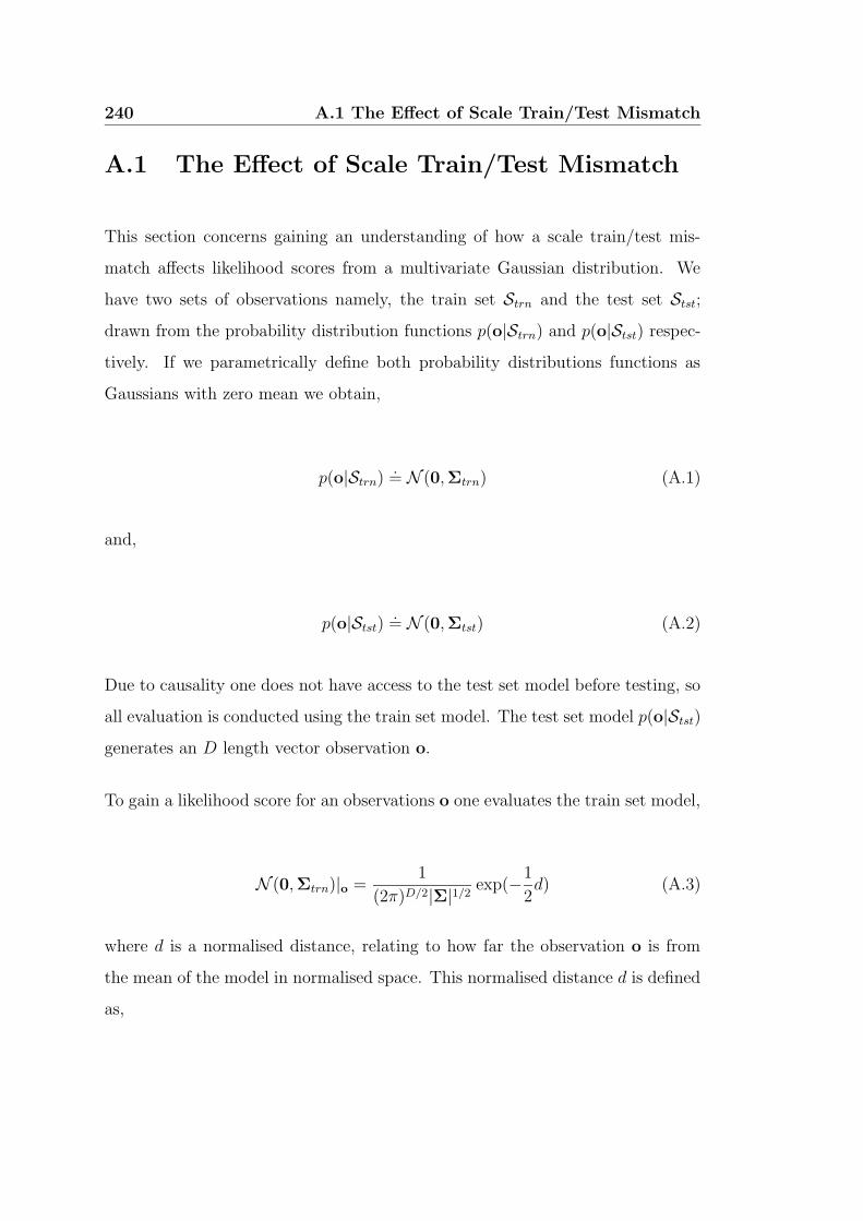
240 A.1 The Effect of Scale Train/Test Mismatch
A.1 The Effect of Scale Train/Test Mismatch
This section concerns gaining an understanding of how a scale train/test mis-
match affects likelihood scores from a multivariate Gaussian distribution. We
have two sets of observations namely, the train set Strn and the test set Stst;
drawn from the probability distribution functions p(o|Strn) and p(o|Stst) respec-
tively. If we parametrically define both probability distributions functions as
Gaussians with zero mean we obtain,
p(o|Strn).= N (0,Σtrn) (A.1)
and,
p(o|Stst).= N (0,Σtst) (A.2)
Due to causality one does not have access to the test set model before testing, so
all evaluation is conducted using the train set model. The test set model p(o|Stst)
generates an D length vector observation o.
To gain a likelihood score for an observations o one evaluates the train set model,
N (0,Σtrn)|o =1
(2π)D/2|Σ|1/2exp(−
1
2d) (A.3)
where d is a normalised distance, relating to how far the observation o is from
the mean of the model in normalised space. This normalised distance d is defined
as,

A.1 The Effect of Scale Train/Test Mismatch 241
d = o′Σ−1trno
= z′z
=D∑
i=1
z2i (A.4)
where z = C′o and C is the whitening transformation [35] derived from the train
covariance matrix Σtrn. The vector z is theD dimensional vector z = [z1, . . . , zD]′.
From [35] one can equate,
Ez′z = tr [E(zz′]
= tr(ΣtstΣ
−1trn
)(A.5)
This section is specifically dealing with scale mismatches between the train and
test sets stemming only from differences in the isotropic variance σ2 such that,
Σtrn = σ2Σtst (A.6)
Of particular interest is the effect changes in σ2 have on the normalised distance d.
One can gain the expectation of normalised distance d in Equation A.7 using
Equations A.4, A.5 and A.6,
Ed =D∑
i=1
Ez2i
= tr(ΣtstΣ−1trn)
= σ2D (A.7)
The variance of the normalised distance d is,
V ard = Ed2 − E2d (A.8)
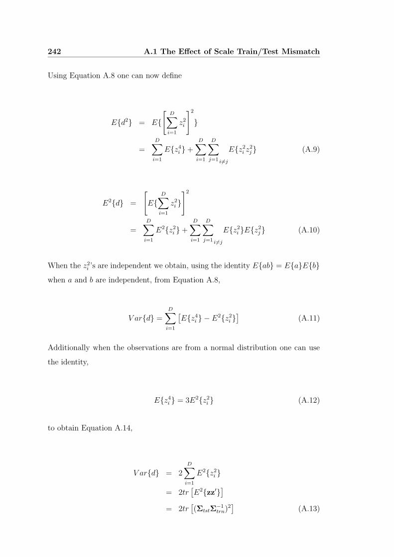
242 A.1 The Effect of Scale Train/Test Mismatch
Using Equation A.8 one can now define
Ed2 = E
[D∑
i=1
z2i
]2
=D∑
i=1
Ez4i +
D∑
i=1
D∑
j=1 i6=j
Ez2i z
2j (A.9)
E2d =
[
ED∑
i=1
z2i
]2
=D∑
i=1
E2z2i +
D∑
i=1
D∑
j=1 i6=j
Ez2i Ez
2j (A.10)
When the z2i ’s are independent we obtain, using the identity Eab = EaEb
when a and b are independent, from Equation A.8,
V ard =D∑
i=1
[Ez4
i − E2z2i
](A.11)
Additionally when the observations are from a normal distribution one can use
the identity,
Ez4i = 3E2z2
i (A.12)
to obtain Equation A.14,
V ard = 2D∑
i=1
E2z2i
= 2tr[E2zz′
]
= 2tr[(ΣtstΣ
−1trn)2
](A.13)

A.1 The Effect of Scale Train/Test Mismatch 243
Again constraining the train/test mismatch to the isotropic scaling found in Equa-
tion A.6, one can substitute Equation A.7,
V ard = 2Dσ4 (A.14)
Equations A.7 and A.14 demonstrate that an isotropic scale mismatch only affects
the statistics of the normalised distance d by a scaling factor.