Audio-Visual Grouplet: Temporal Audio-Visual Interactionsfor General Video Concept Classification

Wei Jiang Alexander C. LouiCorporate Research and Engineering, Eastman Kodak Company, Rochester, NY

{wei.jiang, alexander.loui}@kodak.com

ABSTRACTWe investigate general concept classification in unconstrainedvideos by joint audio-visual analysis. A novel representation,the Audio-Visual Grouplet (AVG), is extracted by studyingthe statistical temporal audio-visual interactions. An AVGis defined as a set of audio and visual codewords that aregrouped together according to their strong temporal corre-lations in videos. The AVGs carry unique audio-visual cuesto represent the video content, based on which an audio-visual dictionary can be constructed for concept classifica-tion. By using the entire AVGs as building elements, theaudio-visual dictionary is much more robust than traditionalvocabularies that use discrete audio or visual codewords.Specifically, we conduct coarse-level foreground/backgroundseparation in both audio and visual channels, and discoverfour types of AVGs by exploring mixed-and-matched tem-poral audio-visual correlations among the following factors:visual foreground, visual background, audio foreground, andaudio background. All of these types of AVGs provide dis-criminative audio-visual patterns for classifying various se-mantic concepts. We extensively evaluate our method overthe large-scale Columbia Consumer Video set. Experimentsdemonstrate that the AVG-based dictionaries can achieveconsistent and significant performance improvements com-pared with other state-of-the-art approaches.

Categories and Subject DescriptorsH.3.1 [Information Storage and Retrieval]: ContentAnalysis and Indexing; H.4.m [Information Systems Ap-plications]: Miscellaneous; H.3.m [Information Storageand Retrieval]: Miscellaneous

General TermsAlgorithms, Experimentation

KeywordsAudio-visual grouplet, video concept classification, temporalaudio-visual interaction, foreground/background separation

∗Area chair: Cees G.M. Snoek

Permission to make digital or hard copies of all or part of this work forpersonal or classroom use is granted without fee provided that copies arenot made or distributed for profit or commercial advantage and that copiesbear this notice and the full citation on the first page. To copy otherwise, torepublish, to post on servers or to redistribute to lists, requires prior specificpermission and/or a fee.MM’11, November 28–December 1, 2011, Scottsdale, Arizona, USA.Copyright 2011 ACM 978-1-4503-0616-4/11/11 ...$10.00.

1. INTRODUCTIONThis paper investigates the problem of automatic classifi-

cation of semantic concepts in generic, unconstrained videos,by joint analysis of audio and visual content. These conceptsinclude general categories, such as scene (e.g., beach), event(e.g., birthday, graduation), location (e.g., playground) andobject (e.g., dog, bird). Generic videos are captured in anunrestricted manner, like those videos taken by consumerson YouTube. This is a difficult problem due to the diversevideo content as well as the challenging conditions such asuneven lighting, clutter, occlusions, and complicated mo-tions of both objects and camera.

Large efforts have been devoted to classify general con-cepts in generic videos, such as TRECVID high-level featureextraction [32] and Columbia Consumer Video (CCV) con-cept classification [18]. Most previous works classify videosin the same way they classify images, using mainly visualinformation. Specifically, visual features are extracted fromeither 2D keyframes or 3D local volumes, and these featuresare treated as individual static descriptors to train conceptclassifiers. Among these methods, the ones using the Bag-of-Words (BoW) representation over 2D or 3D local descriptors(e.g., SIFT [23] or HOG [8]) are considered state-of-the-art,due to the effectiveness of BoW features in classifying ob-jects [13], events [32], and human actions [21].

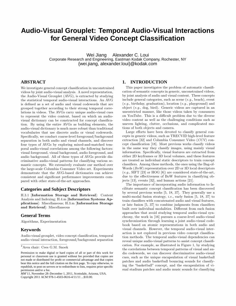
The importance of incorporating audio information to fa-cilitate semantic concept classification has been discoveredby several previous works [5, 18, 37]. They generally use amulti-modal fusion strategy, i.e., early fusion [5, 18, 37] totrain classifiers with concatenated audio and visual features,or late fusion [5, 37] to combine judgments from classifiersbuilt over individual modalities. Different from such fusionapproaches that avoid studying temporal audio-visual syn-chrony, the work in [16] pursues a coarse-level audio-visualsynchronization through learning a joint audio-visual code-book based on atomic representations in both audio andvisual channels. However, the temporal audio-visual inter-action is not explored in previous video concept classifica-tion methods. The temporal audio-visual dependencies canreveal unique audio-visual patterns to assist concept classifi-cation. For example, as illustrated in Figure 1, by studyingthe correlations between temporal patterns of visual and au-dio codewords, we can discover discriminative audio-visualcues, such as the unique encapsulation of visual basketballpatches and audio basketball bouncing sounds for classify-ing the “basketball” concept, and the encapsulation of vi-sual stadium patches and audio music sounds for classifying

. . .

Temporal Patterns of Codeword Occurrences

. . .

. . .

: A Video of “Basketball”2Vtime

. . .

Image Sequence

Audio Spectrogram

. . . 1 1( , )visualPattern V w

1 1( , )audioPattern V w

2 2( , )visualPattern V w

2 2( , )audioPattern V w

1visualw 2

visualw . . .Visual Vocabulary:

1audiow . . .Audio Vocabulary: 2

audiow

Image Sequence

: A Video of “Non-music Performance”1Vtime

. . .

Audio Spectrogram

Figure 1: Discovery of audio-visual patterns through temporal audio-visual interactions. wvisuali and waudio

j are

discrete codewords in visual and audio vocabularies, respectively. By analyzing the correlations between the temporal

histograms of audio and visual codewords, we can discover salient audio-visual cues to represent videos from different

concepts. For example, the highly correlated visual basketball patches and audio basketball bouncing sounds provide

a unique pattern to classify “basketball” videos. The highly correlated visual stadium patches and audio background

music are helpful to classify “non-music performance” videos. In comparison, discrete audio and visual codewords are

less discriminative than such audio-visual cues.

the “non-music performance” concept 1. To the best of ourknowledge, such audio-visual cues have not been studied be-fore in previous literatures.From another perspective, beyond the traditional BoW

representation, structured visual features have been recentlyfound to be effective in many computer vision tasks. Inaddition to the local feature appearance, spatial relationsamong the local patches are incorporated to increase the ro-bustness of the visual representation. The rationale behindthis is that individual local visual patterns tend to be sen-sitive to variations such as changes of illumination, views,scales, and occlusions. In comparison, a set of co-occurrentlocal patterns can be less ambiguous. Along this direction,pairwise spatial constraints among local interest points havebeen used to enhance image registration [12]; various typesof spatial contextual information have been used for objectdetection [10] and action classification [24]; and a groupletrepresentation has been developed to capture discriminativevisual features and their spatial configurations for detectingthe human-object-interaction scenes in images [39].Motivated by the importance of incorporating audio in-

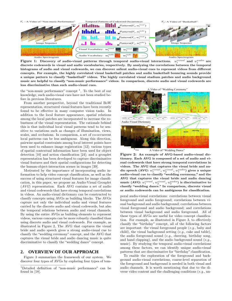
formation to help video concept classification, as well as thesuccess of using structured visual features for image classifi-cation, in this paper, we propose an Audio-Visual Grouplet(AVG) representation. Each AVG contains a set of audioand visual codewords that have strong temporal correlationsin videos. An audio-visual dictionary can be constructed toclassify concepts using AVGs as building blocks. The AVGscapture not only the individual audio and visual featurescarried by the discrete audio and visual codewords, but alsothe temporal relations between audio and visual channels.By using the entire AVGs as building elements to representvideos, various concepts can be more robustly classified thanusing discrete audio and visual codewords. For example, asillustrated in Figure 2, The AVG that captures the visualbride and audio speech gives a strong audio-visual cue toclassify the “wedding ceremony” concept, and the AVG thatcaptures the visual bride and audio dancing music is quitediscriminative to classify the “wedding dance” concept.

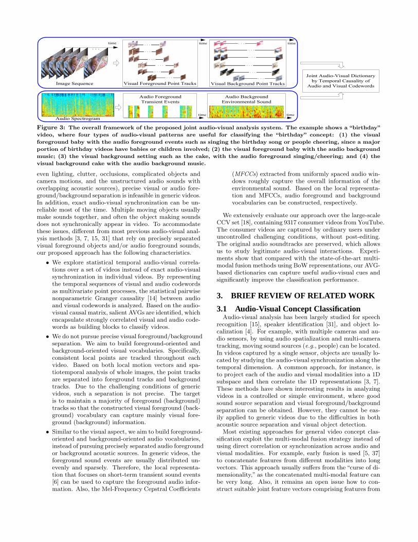
2. OVERVIEW OF OUR APPROACHFigure 3 summarizes the framework of our system. We

discover four types of AVGs by exploring four types of tem-

1Detailed definition of “non-music performance” can befound in [18].

A Video of “Wedding Dance”

time

. . .A Video of “Wedding Ceremony”

time

. . .

Audio-Visual DictionaryAVG 1

visualw 2visualw 1

audiow AVG 3visualw 4

visualw 1audiow AVG 1

visualw 2visualw 2

audiow AVG 5visualw 3

audiow

speechcheering

musiccheering

Figure 2: An example of AVG-based audio-visual dic-

tionary. Each AVG is composed of a set of audio and vi-

sual codewords that have strong temporal correlations in

videos. The AVG that captures the visual bride and au-

dio speech (AVG: wvisual1 , wvisual

2 , waudio1 ) gives a unique

audio-visual cue to classify “wedding ceremony,” and the

AVG that captures the visual bride and audio dancing

music (AVG: wvisual1 , wvisual

2 , waudio2 ) is discriminative to

classify “wedding dance.” In comparison, discrete visual

or audio codewords can be ambiguous for classification.

poral audio-visual correlations: correlations between visualforeground and audio foreground; correlations between vi-sual background and audio background; correlations betweenvisual foreground and audio background; and correlationsbetween visual background and audio foreground. All ofthese types of AVGs are useful for video concept classifica-tion. For example, as illustrated in Figure 3, to effectivelyclassify the “birthday” concept, all of the following factorsare important: the visual foreground people (e.g., baby andchild), the visual background setting (e.g., cake and table),the audio foreground sound (e.g., cheering, birthday song,and hand clapping), and the audio background sound (e.g.,music). By studying the temporal audio-visual correlationsamong these factors, we can identify unique audio-visualpatterns that are discriminative for “birthday”classification.

To enable the exploration of the foreground and back-ground audio-visual correlations, coarse-level separation ofthe foreground and background is needed in both visual andaudio channels. It is worth mentioning that due to the di-verse video content and the challenging conditions (e.g., un-

Joint Audio-Visual Dictionaryby Temporal Causality of

Audio and Visual Codewords

Audio Spectrogram

Audio ForegroundTransient Events

Audio BackgroundEnvironmental Sound

time time

. . .

. . .

. . .

. . .

. . .

Visual Foreground Point Tracks

time

Visual Background Point Tracks

. . .

. . .

. . .

. . .

. . .

. . .

time

Image Sequence

. . .time

. . .

Figure 3: The overall framework of the proposed joint audio-visual analysis system. The example shows a “birthday”

video, where four types of audio-visual patterns are useful for classifying the “birthday” concept: (1) the visual

foreground baby with the audio foreground events such as singing the birthday song or people cheering, since a major

portion of birthday videos have babies or children involved; (2) the visual foreground baby with the audio background

music; (3) the visual background setting such as the cake, with the audio foreground singing/cheering; and (4) the

visual background cake with the audio background music.

even lighting, clutter, occlusions, complicated objects andcamera motions, and the unstructured audio sounds withoverlapping acoustic sources), precise visual or audio fore-ground/background separation is infeasible in generic videos.In addition, exact audio-visual synchronization can be un-reliable most of the time. Multiple moving objects usuallymake sounds together, and often the object making soundsdoes not synchronically appear in video. To accommodatethese issues, different from most previous audio-visual anal-ysis methods [3, 7, 15, 31] that rely on precisely separatedvisual foreground objects and/or audio foreground sounds,our proposed approach has the following characteristics.

• We explore statistical temporal audio-visual correla-tions over a set of videos instead of exact audio-visualsynchronization in individual videos. By representingthe temporal sequences of visual and audio codewordsas multivariate point processes, the statistical pairwisenonparametric Granger causality [14] between audioand visual codewords is analyzed. Based on the audio-visual causal matrix, salient AVGs are identified, whichencapsulate strongly correlated visual and audio code-words as building blocks to classify videos.

• We do not pursue precise visual foreground/backgroundseparation. We aim to build foreground-oriented andbackground-oriented visual vocabularies. Specifically,consistent local points are tracked throughout eachvideo. Based on both local motion vectors and spa-tiotemporal analysis of whole images, the point tracksare separated into foreground tracks and backgroundtracks. Due to the challenging conditions of genericvideos, such a separation is not precise. The targetis to maintain a majority of foreground (background)tracks so that the constructed visual foreground (back-ground) vocabulary can capture mainly visual fore-ground (background) information.

• Similar to the visual aspect, we aim to build foreground-oriented and background-oriented audio vocabularies,instead of pursuing precisely separated audio foregroundor background acoustic sources. In generic videos, theforeground sound events are usually distributed un-evenly and sparsely. Therefore, the local representa-tion that focuses on short-term transient sound events[6] can be used to capture the foreground audio infor-mation. Also, the Mel-Frequency Cepstral Coefficients

(MFCCs) extracted from uniformly spaced audio win-dows roughly capture the overall information of theenvironmental sound. Based on the local representa-tion and MFCCs, audio foreground and backgroundvocabularies can be constructed, respectively.

We extensively evaluate our approach over the large-scaleCCV set [18], containing 9317 consumer videos from YouTube.The consumer videos are captured by ordinary users underuncontrolled challenging conditions, without post-editing.The original audio soundtracks are preserved, which allowsus to study legitimate audio-visual interactions. Experi-ments show that compared with the state-of-the-art multi-modal fusion methods using BoW representations, our AVG-based dictionaries can capture useful audio-visual cues andsignificantly improve the classification performance.

3. BRIEF REVIEW OF RELATED WORK

3.1 Audio-Visual Concept ClassificationAudio-visual analysis has been largely studied for speech

recognition [15], speaker identification [31], and object lo-calization [4]. For example, with multiple cameras and au-dio sensors, by using audio spatialization and multi-cameratracking, moving sound sources (e.g., people) can be located.In videos captured by a single sensor, objects are usually lo-cated by studying the audio-visual synchronization along thetemporal dimension. A common approach, for instance, isto project each of the audio and visual modalities into a 1Dsubspace and then correlate the 1D representations [3, 7].These methods have shown interesting results in analyzingvideos in a controlled or simple environment, where goodsound source separation and visual foreground/backgroundseparation can be obtained. However, they cannot be eas-ily applied to generic videos due to the difficulties in bothacoustic source separation and visual object detection.

Most existing approaches for general video concept clas-sification exploit the multi-modal fusion strategy instead ofusing direct correlation or synchronization across audio andvisual modalities. For example, early fusion is used [5, 37]to concatenate features from different modalities into longvectors. This approach usually suffers from the “curse of di-mensionality,” as the concatenated multi-modal feature canbe very long. Also, it remains an open issue how to con-struct suitable joint feature vectors comprising features from

different modalities with different time scales and differentdistance metrics. In late fusion, individual classifiers arebuilt for each modality separately, and their judgments arecombined to make the final decision. Several combinationstrategies have been used, such as majority voting, linearcombination, super-kernel nonlinear fusion [37], or SVM-based meta-classification combination [22]. However, classi-fier combination remains a basic machine learning problem.The best strategies depend on particular tasks.Recently, an Audio-Visual Atom (AVA) representation has

been developed in [16]. Visual regions are tracked withinshort-term video slices to generate visual atoms, and audioenergy onsets are located to generate audio atoms. Regionalvisual features extracted from visual atoms and spectrogramfeatures extracted from audio atoms are concatenated toform the AVA representation. An audio-visual codebook isconstructed based on the AVAs for concept classification.The audio-visual synchrony is found through learning theaudio-visual codebook. However, the temporal audio-visualinteraction remains unstudied. As illustrated in Figure 1,the temporal audio-visual dependencies can reveal uniqueaudio-visual patterns to assist concept classification.

3.2 Visual Foreground/Background SeparationOne of the most commonly used techniques for separat-

ing foreground moving objects and the static backgroundis background subtraction, where foreground objects are de-tected as the difference between the current frame and a ref-erence image of the static background [11]. Various thresh-old adaptation methods [1] and adaptive background models[33] have been developed. However, these approaches requirea relatively static camera, small illumination change, simpleand stable background scene, and relatively slow object mo-tion. When applied to generic videos for general conceptclassification, the performance is not satisfactory.Motion-based segmentation methods have also been used

to separate moving foreground and static background invideos [20]. The dense optical flow is usually computed tocapture pixel-level motions. Due to the sensitivity to largecamera/object motion and the computation intensity, suchmethods cannot be easily applied to generic videos either.

3.3 Audio Source SeparationReal-world audio signals are combinations of a number

of independent sound sources, such as various instrumen-tal sounds, human voices, natural sounds, etc. Ideally, onewould like to recover each source signal. However, this taskis very challenging in generic videos, because only a singleaudio channel is available, and realistic soundtracks haveunrestricted content from an unknown number of unstruc-tured, overlapping acoustic sources.Early Blind Audio Source Separation (BASS) methods

separate audio sources that are recorded with multiple mi-crophones [28]. Later on, several approaches have been de-veloped to separate single-channel audio, such as the fac-torial HMM methods [30] and the spectral decompositionmethods [35]. Recently, the visual information has been in-corporated to assist BASS [36], where the audio-video syn-chrony is used as side information. However, soundtracksstudied by these methods are mostly mixtures of humanvoices or instrumental sounds with very limited backgroundnoise. When applied to generic videos, existing BASS meth-ods cannot perform satisfactorily.

4. VISUAL PROCESSWe conduct SIFT point tracking within each video, based

on which foreground-oriented and background-oriented tem-poral visual patterns are generated. The following detailsthe processing stages.

4.1 Excluding Bad Video SegmentsVideo shot boundary detection and bad video segment

elimination are general preprocessing steps for video analy-sis. Each raw video is segmented into several parts accordingto the detected shot boundaries with a single shot in eachpart. Next, segments with very large camera motion are ex-cluded from analysis. It is worth mentioning that in our case,these steps can actually be skipped, because we process con-sumer videos that have a single long shot per video, and theSIFT point tracking can automatically exclude bad segmentsby generating few tracks over such segments. However, westill recommend these preprocessing steps to accommodatea large variety of generic videos.

4.2 SIFT-based Point TrackingWe use Lowe’s 128-dim SIFT descriptor with the DoG in-

terest point detector [23]. SIFT features are first extractedfrom a set of uniformly sampled image frames with a sam-pling rate of 6 fps (frames per second) 2. Then for adjacentimage frames, pairs of matching SIFT features are foundbased on the Euclidean distance of their feature vectors,by also using Lowe’s method to discard ambiguous matches[23]. After that, along the temporal dimension, the match-ing pairs are connected into a set of SIFT point tracks, wheredifferent point tracks can start from different image framesand last variable lengths. This 6 fps sampling rate is empir-ically determined by considering both the computation costand the ability of SIFT matching. In general, increasingthe sampling rate will decrease the chance of missing pointtracks, with the price of increased computation.

Each SIFT point track is represented by a 136-dim featurevector. This feature vector is composed by a 128-dim SIFTvector concatenated with an 8-dim motion vector. The SIFTvector is the averaged SIFT features of all SIFT points inthe track. The motion vector is the averaged Histogram ofOriented Motion (HOM) along the track. That is, for eachadjacent matching pair in the track, we compute the speedand direction of the local motion vector. By quantizing the2D motion space into 8 bins (corresponding to 8 directions),an 8-dim HOM feature is computed where the value overeach bin is the averaged speed of the motion vectors fromthe track moving along this direction.

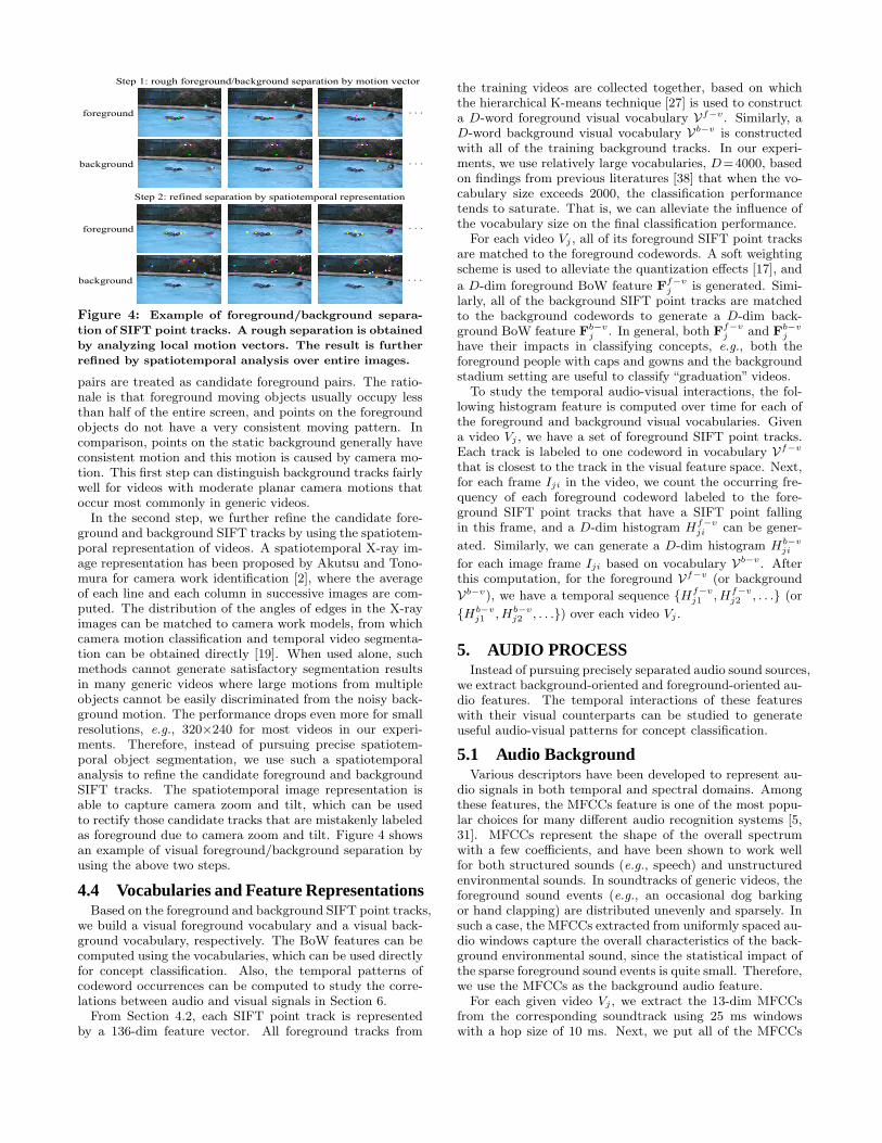
4.3 Foreground/Background SeparationOnce the set of SIFT point tracks are obtained, we sep-

arate them as foreground or background with the followingtwo steps, as illustrated in Figure 4. First, for two adjacentframes Ii and Ii+1, we roughly separate their matching SIFTpairs into candidate foreground and background pairs basedon the motion vectors. Specifically, we group these matchingpairs by hierarchical clustering, where the grouping criterionis that pairs within a cluster have roughly the same movingdirection and speed. Those SIFT pairs in the biggest clus-ter are treated as candidate background pairs, and all other

2In our experiment, the typical frame rate of videos is 30fps. Typically we sample 1 frame from every 5 frames.

Step 1: rough foreground/background separation by motion vector

. . .

. . .

foreground

background

Step 2: refined separation by spatiotemporal representation

. . .

. . .

foreground

background

Figure 4: Example of foreground/background separa-

tion of SIFT point tracks. A rough separation is obtained

by analyzing local motion vectors. The result is further

refined by spatiotemporal analysis over entire images.

pairs are treated as candidate foreground pairs. The ratio-nale is that foreground moving objects usually occupy lessthan half of the entire screen, and points on the foregroundobjects do not have a very consistent moving pattern. Incomparison, points on the static background generally haveconsistent motion and this motion is caused by camera mo-tion. This first step can distinguish background tracks fairlywell for videos with moderate planar camera motions thatoccur most commonly in generic videos.In the second step, we further refine the candidate fore-

ground and background SIFT tracks by using the spatiotem-poral representation of videos. A spatiotemporal X-ray im-age representation has been proposed by Akutsu and Tono-mura for camera work identification [2], where the averageof each line and each column in successive images are com-puted. The distribution of the angles of edges in the X-rayimages can be matched to camera work models, from whichcamera motion classification and temporal video segmenta-tion can be obtained directly [19]. When used alone, suchmethods cannot generate satisfactory segmentation resultsin many generic videos where large motions from multipleobjects cannot be easily discriminated from the noisy back-ground motion. The performance drops even more for smallresolutions, e.g., 320×240 for most videos in our experi-ments. Therefore, instead of pursuing precise spatiotem-poral object segmentation, we use such a spatiotemporalanalysis to refine the candidate foreground and backgroundSIFT tracks. The spatiotemporal image representation isable to capture camera zoom and tilt, which can be usedto rectify those candidate tracks that are mistakenly labeledas foreground due to camera zoom and tilt. Figure 4 showsan example of visual foreground/background separation byusing the above two steps.

4.4 Vocabularies and Feature RepresentationsBased on the foreground and background SIFT point tracks,

we build a visual foreground vocabulary and a visual back-ground vocabulary, respectively. The BoW features can becomputed using the vocabularies, which can be used directlyfor concept classification. Also, the temporal patterns ofcodeword occurrences can be computed to study the corre-lations between audio and visual signals in Section 6.From Section 4.2, each SIFT point track is represented

by a 136-dim feature vector. All foreground tracks from

the training videos are collected together, based on whichthe hierarchical K-means technique [27] is used to constructa D-word foreground visual vocabulary Vf−v. Similarly, aD-word background visual vocabulary Vb−v is constructedwith all of the training background tracks. In our experi-ments, we use relatively large vocabularies, D=4000, basedon findings from previous literatures [38] that when the vo-cabulary size exceeds 2000, the classification performancetends to saturate. That is, we can alleviate the influence ofthe vocabulary size on the final classification performance.

For each video Vj , all of its foreground SIFT point tracksare matched to the foreground codewords. A soft weightingscheme is used to alleviate the quantization effects [17], and

a D-dim foreground BoW feature Ff−vj is generated. Simi-

larly, all of the background SIFT point tracks are matchedto the background codewords to generate a D-dim back-ground BoW feature Fb−v

j . In general, both Ff−vj and Fb−v

j

have their impacts in classifying concepts, e.g., both theforeground people with caps and gowns and the backgroundstadium setting are useful to classify “graduation” videos.

To study the temporal audio-visual interactions, the fol-lowing histogram feature is computed over time for each ofthe foreground and background visual vocabularies. Givena video Vj , we have a set of foreground SIFT point tracks.Each track is labeled to one codeword in vocabulary Vf−v

that is closest to the track in the visual feature space. Next,for each frame Iji in the video, we count the occurring fre-quency of each foreground codeword labeled to the fore-ground SIFT point tracks that have a SIFT point fallingin this frame, and a D-dim histogram Hf−v

ji can be gener-

ated. Similarly, we can generate a D-dim histogram Hb−vji

for each image frame Iji based on vocabulary Vb−v. Afterthis computation, for the foreground Vf−v (or background

Vb−v), we have a temporal sequence {Hf−vj1 , Hf−v

j2 , . . .} (or

{Hb−vj1 , Hb−v

j2 , . . .}) over each video Vj .

5. AUDIO PROCESSInstead of pursuing precisely separated audio sound sources,

we extract background-oriented and foreground-oriented au-dio features. The temporal interactions of these featureswith their visual counterparts can be studied to generateuseful audio-visual patterns for concept classification.

5.1 Audio BackgroundVarious descriptors have been developed to represent au-

dio signals in both temporal and spectral domains. Amongthese features, the MFCCs feature is one of the most popu-lar choices for many different audio recognition systems [5,31]. MFCCs represent the shape of the overall spectrumwith a few coefficients, and have been shown to work wellfor both structured sounds (e.g., speech) and unstructuredenvironmental sounds. In soundtracks of generic videos, theforeground sound events (e.g., an occasional dog barkingor hand clapping) are distributed unevenly and sparsely. Insuch a case, the MFCCs extracted from uniformly spaced au-dio windows capture the overall characteristics of the back-ground environmental sound, since the statistical impact ofthe sparse foreground sound events is quite small. Therefore,we use the MFCCs as the background audio feature.

For each given video Vj , we extract the 13-dim MFCCsfrom the corresponding soundtrack using 25 ms windowswith a hop size of 10 ms. Next, we put all of the MFCCs

from all training videos together, on top of which the hierar-chical K-means technique [27] is used to construct a D-wordbackground audio vocabulary Vb−a. Similar to visual-basedprocessing, we compute two different histogram-like featuresbased on Vb−a. First, we generate a BoW feature Fb−a

j foreach video Vj by matching the MFCCs in the video to code-words in the vocabulary and conducting soft weighting. ThisBoW feature can be used directly for classifying concepts.Second, to study the audio-visual correlation, a temporalaudio histogram sequence {Hb−a

j1 , Hb−aj2 , . . .} is generated for

each video Vj as follows. Each MFCC vector is labeled toone codeword in the audio background vocabulary Vb−a thatis closest to the MFCC vector. Next, for each sampled imageframe Iji in the video, we take a 200 ms window centeredon this frame. Then we count the occurring frequency ofthe codewords labeled to the MFCCs that fall into this win-dow, and a D-dim histogram Hb−a

ji can be generated. This

Hb−aji can be considered as temporally synchronized with the

visual-based histograms Hf−vji or Hb−v

ji .

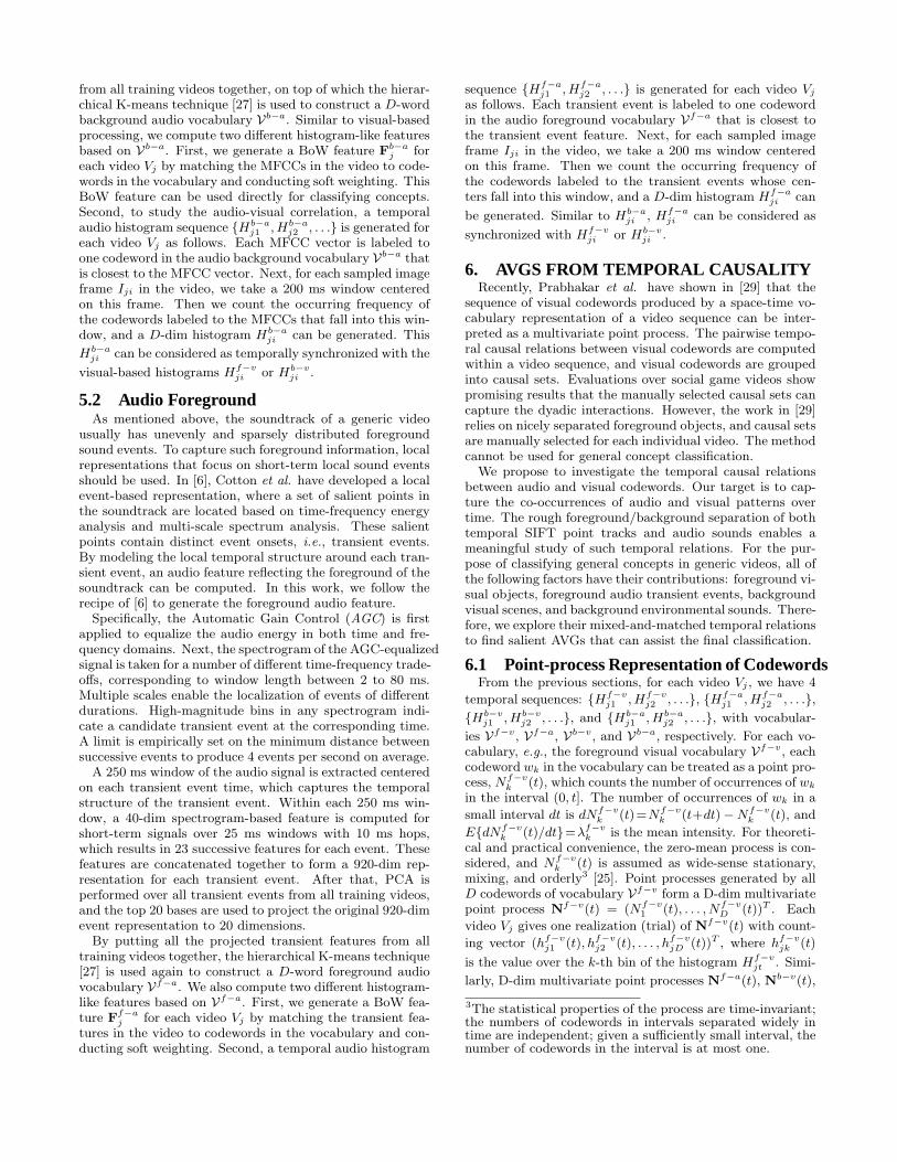
5.2 Audio ForegroundAs mentioned above, the soundtrack of a generic video

usually has unevenly and sparsely distributed foregroundsound events. To capture such foreground information, localrepresentations that focus on short-term local sound eventsshould be used. In [6], Cotton et al. have developed a localevent-based representation, where a set of salient points inthe soundtrack are located based on time-frequency energyanalysis and multi-scale spectrum analysis. These salientpoints contain distinct event onsets, i.e., transient events.By modeling the local temporal structure around each tran-sient event, an audio feature reflecting the foreground of thesoundtrack can be computed. In this work, we follow therecipe of [6] to generate the foreground audio feature.Specifically, the Automatic Gain Control (AGC) is first

applied to equalize the audio energy in both time and fre-quency domains. Next, the spectrogram of the AGC-equalizedsignal is taken for a number of different time-frequency trade-offs, corresponding to window length between 2 to 80 ms.Multiple scales enable the localization of events of differentdurations. High-magnitude bins in any spectrogram indi-cate a candidate transient event at the corresponding time.A limit is empirically set on the minimum distance betweensuccessive events to produce 4 events per second on average.A 250 ms window of the audio signal is extracted centered

on each transient event time, which captures the temporalstructure of the transient event. Within each 250 ms win-dow, a 40-dim spectrogram-based feature is computed forshort-term signals over 25 ms windows with 10 ms hops,which results in 23 successive features for each event. Thesefeatures are concatenated together to form a 920-dim rep-resentation for each transient event. After that, PCA isperformed over all transient events from all training videos,and the top 20 bases are used to project the original 920-dimevent representation to 20 dimensions.By putting all the projected transient features from all

training videos together, the hierarchical K-means technique[27] is used again to construct a D-word foreground audiovocabulary Vf−a. We also compute two different histogram-like features based on Vf−a. First, we generate a BoW fea-ture Ff−a

j for each video Vj by matching the transient fea-tures in the video to codewords in the vocabulary and con-ducting soft weighting. Second, a temporal audio histogram

sequence {Hf−aj1 , Hf−a

j2 , . . .} is generated for each video Vj

as follows. Each transient event is labeled to one codewordin the audio foreground vocabulary Vf−a that is closest tothe transient event feature. Next, for each sampled imageframe Iji in the video, we take a 200 ms window centeredon this frame. Then we count the occurring frequency ofthe codewords labeled to the transient events whose cen-ters fall into this window, and a D-dim histogram Hf−a

ji can

be generated. Similar to Hb−aji , Hf−a

ji can be considered as

synchronized with Hf−vji or Hb−v

ji .

6. AVGS FROM TEMPORAL CAUSALITYRecently, Prabhakar et al. have shown in [29] that the

sequence of visual codewords produced by a space-time vo-cabulary representation of a video sequence can be inter-preted as a multivariate point process. The pairwise tempo-ral causal relations between visual codewords are computedwithin a video sequence, and visual codewords are groupedinto causal sets. Evaluations over social game videos showpromising results that the manually selected causal sets cancapture the dyadic interactions. However, the work in [29]relies on nicely separated foreground objects, and causal setsare manually selected for each individual video. The methodcannot be used for general concept classification.

We propose to investigate the temporal causal relationsbetween audio and visual codewords. Our target is to cap-ture the co-occurrences of audio and visual patterns overtime. The rough foreground/background separation of bothtemporal SIFT point tracks and audio sounds enables ameaningful study of such temporal relations. For the pur-pose of classifying general concepts in generic videos, all ofthe following factors have their contributions: foreground vi-sual objects, foreground audio transient events, backgroundvisual scenes, and background environmental sounds. There-fore, we explore their mixed-and-matched temporal relationsto find salient AVGs that can assist the final classification.

6.1 Point-process Representation of CodewordsFrom the previous sections, for each video Vj , we have 4

temporal sequences: {Hf−vj1 , Hf−v

j2 , . . .}, {Hf−aj1 , Hf−a

j2 , . . .},{Hb−v

j1 , Hb−vj2 , . . .}, and {Hb−a

j1 , Hb−aj2 , . . .}, with vocabular-

ies Vf−v, Vf−a, Vb−v, and Vb−a, respectively. For each vo-cabulary, e.g., the foreground visual vocabulary Vf−v, eachcodeword wk in the vocabulary can be treated as a point pro-cess, Nf−v

k (t), which counts the number of occurrences of wk

in the interval (0, t]. The number of occurrences of wk in a

small interval dt is dNf−vk (t)=Nf−v

k (t+dt)−Nf−vk (t), and

E{dNf−vk (t)/dt}=λf−v

k is the mean intensity. For theoreti-cal and practical convenience, the zero-mean process is con-sidered, and Nf−v

k (t) is assumed as wide-sense stationary,mixing, and orderly3 [25]. Point processes generated by allD codewords of vocabulary Vf−v form a D-dim multivariatepoint process Nf−v(t) = (Nf−v

1 (t), . . . , Nf−vD (t))T . Each

video Vj gives one realization (trial) of Nf−v(t) with count-

ing vector (hf−vj1 (t), hf−v

j2 (t), . . . , hf−vjD (t))T , where hf−v

jk (t)

is the value over the k-th bin of the histogram Hf−vjt . Simi-

larly, D-dim multivariate point processes Nf−a(t), Nb−v(t),

3The statistical properties of the process are time-invariant;the numbers of codewords in intervals separated widely intime are independent; given a sufficiently small interval, thenumber of codewords in the interval is at most one.

and Nb−a(t) can be generated for vocabularies Vf−a, Vb−v,and Vb−a, respectively.

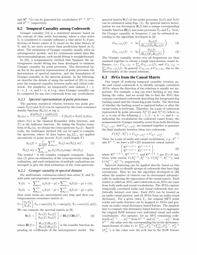
6.2 Temporal Causality among CodewordsGranger causality [14] is a statistical measure based on

the concept of time series forecasting, where a time seriesY1 is considered to causally influence a time series Y2 if pre-dictions of future values of Y2 based on the joint history ofY1 and Y2 are more accurate than predictions based on Y2

alone. The estimation of Granger causality usually relies onautoregressive models, and for continuous-valued data likeelectroencephalogram, such model fitting is straightforward.In [25], a nonparametric method that bypasses the au-

toregressive model fitting has been developed to estimateGranger causality for point processes. The theoretical ba-sis lies in the spectral representation of point processes, thefactorization of spectral matrices, and the formulation ofGranger causality in the spectral domain. In the following,we describe the details of using the method of [25] to com-pute the temporal causality between audio and visual code-words. For simplicity, we temporarily omit indexes f − v,b− v, f − a, and b− a, w.l.o.g., since Granger causality canbe computed for any two codewords from any vocabularies.

6.2.1 Spectral representation of point processesThe pairwise statistical relation between two point pro-

cessesNk(t) andNl(t) can be captured by the cross-covariancedensity function Rkl(u) at lag u:

Rkl(u) =E{dNk(t+ u)dNl(t)}

dudt− I [Nk(t)=Nl(t)]λkδ(u),

where δ(u) is the classical Kronecker delta function, andI[·] is the indicator function. By taking the Fourier trans-form of Rkl(u), we obtain the cross-spectrum Skl(f). Specif-ically, the multitaper method [34] can be used to computethe spectrum, where M data tapers {qm}Mm=1 are appliedsuccessively to point process Nk(t) (with length T ):

Skl(f) =1

2πMT

∑M

m=1Nk(f,m)Nl(f,m)∗, (1)

Nk(f,m) =∑T

tp=1qm(tp)Nk(tp)exp(−2πiftp).

The symbol ∗ is the complex conjugate transpose. Equa-tion (1) gives an estimation of the cross-spectrum using onerealization, and such estimations of multiple realizations areaveraged to give the final estimation of the cross-spectrum.

6.2.2 Granger causality in spectral domainFor multivariate continuous-valued time series Y1 and Y2

with joint autoregressive representations:

Y1(t) =∑∞

p=1apY1(t− p) +

∑∞p=1

bpY2(t− p) + ε(t),

Y2(t) =∑∞

p=1cpY2(t− p) +

∑∞p=1

dpY1(t− p) + η(t),

their noise terms are uncorrelated over time and their con-temporaneous covariance matrix is:

Σ=

[Σ2Υ2

Υ2Γ2

],Σ2=var(ε(t)),Γ2=var(η(t)),Υ2=cov(ε(t), η(t)).

We can compute the spectral matrix as [9]:

S(f) =

[S11(f) S12(f)S21(f) S22(f)

]= H(f)ΣH(f)∗, (2)

where H(f)=

[H11(f)H12(f)H21(f)H22(f)

]is the transfer function de-

pending on coefficients of the autoregressive model. The

spectral matrix S(f) of two point processes Nk(t) and Nl(t)can be estimated using Eqn. (1). By spectral matrix factor-ization we can decompose S(f) into a unique corresponding

transfer function H(f) and noise processes Σ2 and Γ2. Next,the Granger causality at frequency f can be estimated ac-cording to the algorithm developed in [9]:

GNl→Nk (f) = ln

(Skk(f)

Hkk(f)Σ2Hkk(f)∗

), (3)

GNk→Nl(f) = ln

(Sll(f)

Hll(f)Γ2Hll(f)∗

). (4)

The Granger causality scores over all frequencies are thensummed together to obtain a single time-domain causal in-fluence, i.e., CNk→Nl =

∑f GNk→Nl(f), and CNl→Nk =∑

f GNl→Nk (f). In general, CNk→Nl �=CNl→Nk , due to thedirectionality of the causal relations.

6.3 AVGs from the Causal MatrixOur target of studying temporal causality between au-

dio and visual codewords is to identify strongly correlatedAVGs, where the direction of the relations is usually not im-portant. For example, a dog can start barking at any timeduring the video, and we would like to find the AVG thatcontains correlated codewords describing the foreground dogbarking sound and the visual dog point tracks. The directionof whether the barking sound is captured before or after thevisual tracks is irrelevant. Therefore, for a pair of codewordsrepresented by point processes N

skk (t) and N

sll (t) (where sk

or sl is one of the following f − v, f − a, b − v, and b − a,indicating the vocabularies the codeword comes from), thenonparametric Granger causality scores from both directionsCN

skk

→Nsll

and CNsll

→Nskk

are summed together to generate

the final similarity between these two codewords:

C(Nskk , N

sll ) = CN

skk

→Nsll

+ CNsll

→Nskk

. (5)

Then, for a pair of audio and visual vocabularies, e.g., Vf−v

and Vf−a, we have a 2D×2D symmetric causal matrix:[Cf−v,f−v Cf−v,f−a

Cf−a,f−v Cf−a,f−a

], (6)

where Cf−v,f−v, Cf−a,f−a, and Cf−v,f−a are D×D ma-trices with entries C(Nf−v

k , Nf−vl ), C(Nf−a

k , Nf−al ), and

C(Nf−vk , Nf−a

l ), respectively.Spectral clustering can be applied directly based on this

causal matrix to identify groups of codewords that have highcorrelations. Here we use the algorithm developed in [26]where the number of clusters can be determined automati-cally by analyzing the eigenvalues of the causal matrix. Eachcluster is called an AVG, and codewords in an AVG can comefrom both audio and visual vocabularies. The AVGs capturetemporally correlated audio and visual codewords that sta-tistically interact over time. Each AVG can be treated asan audio-visual pattern, and all AVGs form an audio-visualdictionary. For a given video Vj , the original SIFT pointtracks and audio features can be mapped to AVGs and gen-erate an audio-visual dictionary-based feature. The simplestway to compute this dictionary-based feature is to aggregatethe original BoW features over individual visual and audiovocabularies. For instance, for an AVG containing code-words wf−a

1 , . . . , wf−an from Vf−a, and wf−v

1 , . . . , wf−vm from

Vf−v, the value over the corresponding bin in the dictionary-based feature of video Vj is:

∑np=1F

f−ajp +

∑mp=1F

f−vjp . F f−a

jp

(F f−vjp ) is the value over the p-th bin in the BoW feature

Ff−aj (Ff−v

j ) over Vf−a (Vf−v). Classifiers such as SVMscan be trained using this feature for concept classification.

A total of four audio-visual dictionaries are generated inthis work, by studying the temporal causal relations betweendifferent types of audio and visual codewords. They are: dic-tionary Df−v,f−a by correlating Vf−v and Vf−a, Db−v,b−a

by correlating Vb−v and Vb−a, Df−v,b−a by correlating Vf−v

and Vb−a, and Db−v,f−a by correlating Vb−v and Vf−a. Asillustrated in Figure 3, all of these correlations reveal usefulaudio-visual patterns for classifying concepts.

7. EXPERIMENTSWe evaluate our algorithm over the large-scale CCV set

[18], containing 9317 consumer videos from YouTube. Thesevideos are captured by ordinary users under unrestrictedchallenging conditions, without post-editing. The originalaudio soundtracks are preserved, in contrast to other large-scale news or movie video sets [21, 32]. This allows us tostudy legitimate audio-visual interactions. Each video ismanually labeled to 20 semantic concepts by using Ama-zon Mechanical Turk. More details about the data set andcategory definitions can be found in [18]. Our experimentstake similar settings as [18], i.e., we use the same training(4659 videos) and test (4658 videos) sets, and one-versus-allχ2-kernel SVM classifiers. The performance is measured byAverage Precision (AP, the area under uninterpolated PRcurve) and Mean AP (MAP, averaged AP across concepts).

7.1 Performance of Concept ClassificationTo demonstrate the effectiveness of our method, we first

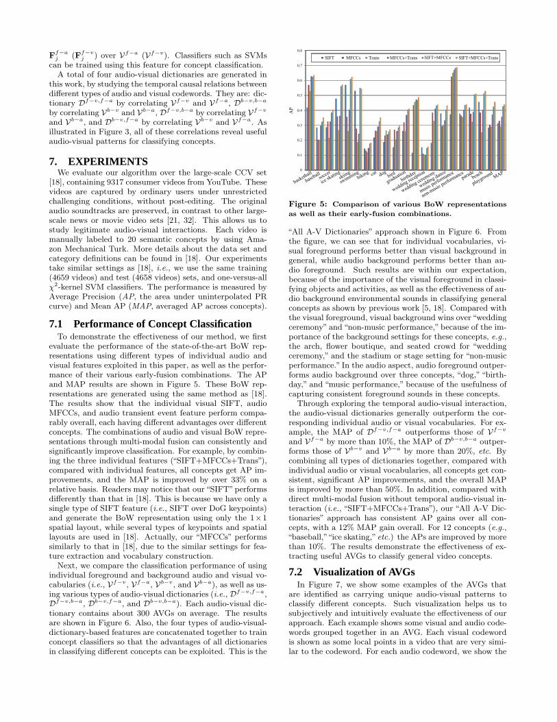
evaluate the performance of the state-of-the-art BoW rep-resentations using different types of individual audio andvisual features exploited in this paper, as well as the perfor-mance of their various early-fusion combinations. The APand MAP results are shown in Figure 5. These BoW rep-resentations are generated using the same method as [18].The results show that the individual visual SIFT, audioMFCCs, and audio transient event feature perform compa-rably overall, each having different advantages over differentconcepts. The combinations of audio and visual BoW repre-sentations through multi-modal fusion can consistently andsignificantly improve classification. For example, by combin-ing the three individual features (“SIFT+MFCCs+Trans”),compared with individual features, all concepts get AP im-provements, and the MAP is improved by over 33% on arelative basis. Readers may notice that our“SIFT”performsdifferently than that in [18]. This is because we have only asingle type of SIFT feature (i.e., SIFT over DoG keypoints)and generate the BoW representation using only the 1×1spatial layout, while several types of keypoints and spatiallayouts are used in [18]. Actually, our “MFCCs” performssimilarly to that in [18], due to the similar settings for fea-ture extraction and vocabulary construction.

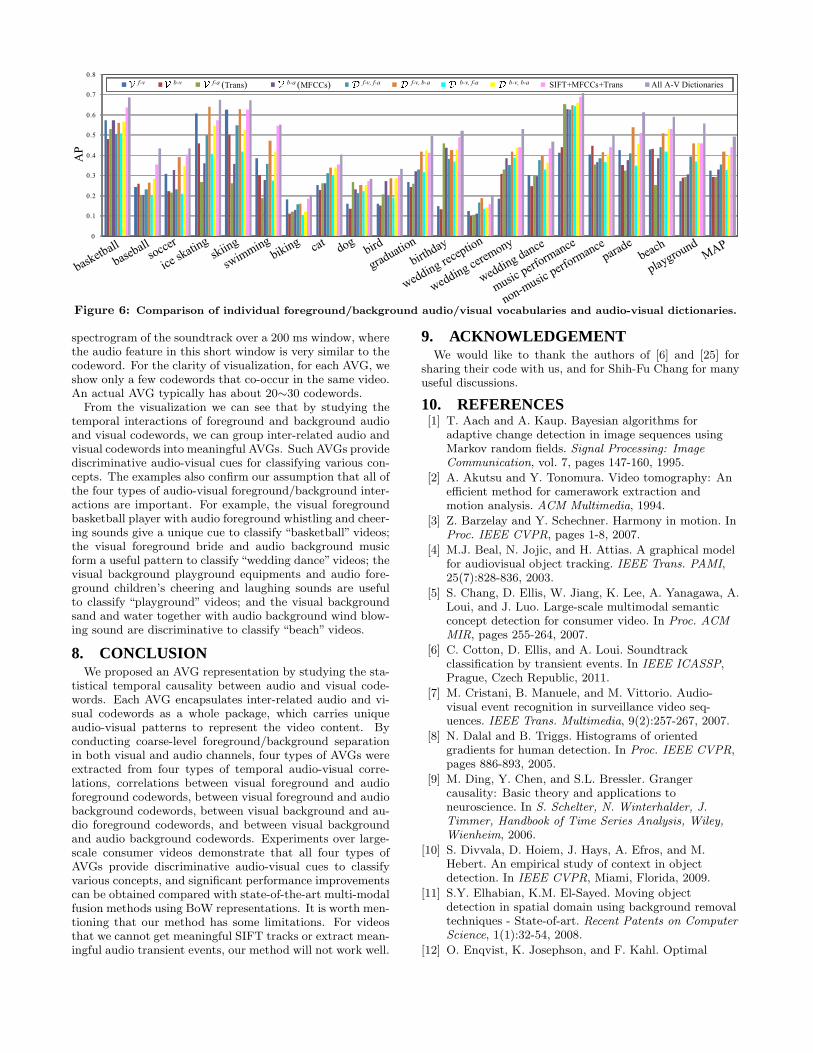
Next, we compare the classification performance of usingindividual foreground and background audio and visual vo-cabularies (i.e., Vf−v, Vf−a, Vb−v, and Vb−a), as well as us-ing various types of audio-visual dictionaries (i.e., Df−v,f−a,Df−v,b−a, Db−v,f−a, and Db−v,b−a). Each audio-visual dic-tionary contains about 300 AVGs on average. The resultsare shown in Figure 6. Also, the four types of audio-visual-dictionary-based features are concatenated together to trainconcept classifiers so that the advantages of all dictionariesin classifying different concepts can be exploited. This is the

0

0.1

0.2

0.3

0.4

0.5

0.6

0.7

0.8

SIFT MFCC Trans MFCC+Trans SIFT+MFCC SIFT+MFCC+Trans

basketball

AP

SIFT MFCCs Trans MFCCs+Trans SIFT+MFCCs SIFT+MFCCs+Trans

baseballsoccer

ice skatingskiing

swimmingbiking cat dog

bird

graduationbirth

day

wedding reception

wedding ceremony

wedding dance

music performance

non-music performanceparade

beach

playgroundMAP

Figure 5: Comparison of various BoW representations

as well as their early-fusion combinations.

“All A-V Dictionaries” approach shown in Figure 6. Fromthe figure, we can see that for individual vocabularies, vi-sual foreground performs better than visual background ingeneral, while audio background performs better than au-dio foreground. Such results are within our expectation,because of the importance of the visual foreground in classi-fying objects and activities, as well as the effectiveness of au-dio background environmental sounds in classifying generalconcepts as shown by previous work [5, 18]. Compared withthe visual foreground, visual background wins over“weddingceremony” and “non-music performance,” because of the im-portance of the background settings for these concepts, e.g.,the arch, flower boutique, and seated crowd for “weddingceremony,” and the stadium or stage setting for “non-musicperformance.” In the audio aspect, audio foreground outper-forms audio background over three concepts, “dog,”“birth-day,” and “music performance,” because of the usefulness ofcapturing consistent foreground sounds in these concepts.

Through exploring the temporal audio-visual interaction,the audio-visual dictionaries generally outperform the cor-responding individual audio or visual vocabularies. For ex-ample, the MAP of Df−v,f−a outperforms those of Vf−v

and Vf−a by more than 10%, the MAP of Db−v,b−a outper-forms those of Vb−v and Vb−a by more than 20%, etc. Bycombining all types of dictionaries together, compared withindividual audio or visual vocabularies, all concepts get con-sistent, significant AP improvements, and the overall MAPis improved by more than 50%. In addition, compared withdirect multi-modal fusion without temporal audio-visual in-teraction (i.e., “SIFT+MFCCs+Trans”), our “All A-V Dic-tionaries” approach has consistent AP gains over all con-cepts, with a 12% MAP gain overall. For 12 concepts (e.g.,“baseball,”“ice skating,”etc.) the APs are improved by morethan 10%. The results demonstrate the effectiveness of ex-tracting useful AVGs to classify general video concepts.

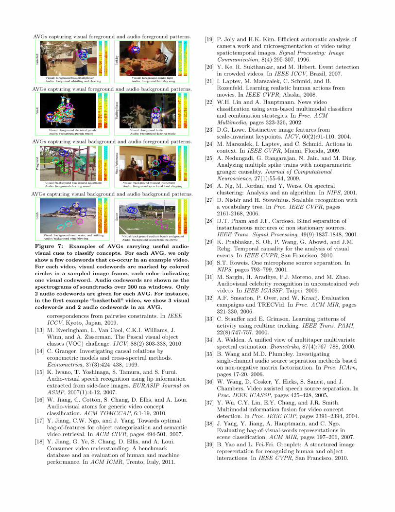
7.2 Visualization of AVGsIn Figure 7, we show some examples of the AVGs that

are identified as carrying unique audio-visual patterns toclassify different concepts. Such visualization helps us tosubjectively and intuitively evaluate the effectiveness of ourapproach. Each example shows some visual and audio code-words grouped together in an AVG. Each visual codewordis shown as some local points in a video that are very simi-lar to the codeword. For each audio codeword, we show the

0

0.1

0.2

0.3

0.4

0.5

0.6

0.7

0.8Vf-v Vb-v Vf-a (Transient) V-b-a (MFCCs) Df-v,f-a Df-v,b-a Db-v,f-a Db-v,b-a SIFT+MFCCs+Transient All A-V Dictionaries

basketball

AP

baseballsoccer

ice skatingskiing

swimmingbiking cat dog bird

graduationbirth

day

wedding reception

wedding ceremony

wedding dance

music performance

non-music performanceparade

beach

playgroundMAP

f-v b-v f-a (Trans) b-a (MFCCs) f-v, f-a f-v, b-a b-v, f-a b-v, b-a SIFT+MFCCs+Trans All A-V Dictionaries

Figure 6: Comparison of individual foreground/background audio/visual vocabularies and audio-visual dictionaries.

spectrogram of the soundtrack over a 200 ms window, wherethe audio feature in this short window is very similar to thecodeword. For the clarity of visualization, for each AVG, weshow only a few codewords that co-occur in the same video.An actual AVG typically has about 20∼30 codewords.

From the visualization we can see that by studying thetemporal interactions of foreground and background audioand visual codewords, we can group inter-related audio andvisual codewords into meaningful AVGs. Such AVGs providediscriminative audio-visual cues for classifying various con-cepts. The examples also confirm our assumption that all ofthe four types of audio-visual foreground/background inter-actions are important. For example, the visual foregroundbasketball player with audio foreground whistling and cheer-ing sounds give a unique cue to classify “basketball” videos;the visual foreground bride and audio background musicform a useful pattern to classify “wedding dance”videos; thevisual background playground equipments and audio fore-ground children’s cheering and laughing sounds are usefulto classify “playground” videos; and the visual backgroundsand and water together with audio background wind blow-ing sound are discriminative to classify “beach” videos.

8. CONCLUSIONWe proposed an AVG representation by studying the sta-

tistical temporal causality between audio and visual code-words. Each AVG encapsulates inter-related audio and vi-sual codewords as a whole package, which carries uniqueaudio-visual patterns to represent the video content. Byconducting coarse-level foreground/background separationin both visual and audio channels, four types of AVGs wereextracted from four types of temporal audio-visual corre-lations, correlations between visual foreground and audioforeground codewords, between visual foreground and audiobackground codewords, between visual background and au-dio foreground codewords, and between visual backgroundand audio background codewords. Experiments over large-scale consumer videos demonstrate that all four types ofAVGs provide discriminative audio-visual cues to classifyvarious concepts, and significant performance improvementscan be obtained compared with state-of-the-art multi-modalfusion methods using BoW representations. It is worth men-tioning that our method has some limitations. For videosthat we cannot get meaningful SIFT tracks or extract mean-ingful audio transient events, our method will not work well.

9. ACKNOWLEDGEMENTWe would like to thank the authors of [6] and [25] for

sharing their code with us, and for Shih-Fu Chang for manyuseful discussions.

10. REFERENCES[1] T. Aach and A. Kaup. Bayesian algorithms for

adaptive change detection in image sequences usingMarkov random fields. Signal Processing: ImageCommunication, vol. 7, pages 147-160, 1995.

[2] A. Akutsu and Y. Tonomura. Video tomography: Anefficient method for camerawork extraction andmotion analysis. ACM Multimedia, 1994.

[3] Z. Barzelay and Y. Schechner. Harmony in motion. InProc. IEEE CVPR, pages 1-8, 2007.

[4] M.J. Beal, N. Jojic, and H. Attias. A graphical modelfor audiovisual object tracking. IEEE Trans. PAMI,25(7):828-836, 2003.

[5] S. Chang, D. Ellis, W. Jiang, K. Lee, A. Yanagawa, A.Loui, and J. Luo. Large-scale multimodal semanticconcept detection for consumer video. In Proc. ACMMIR, pages 255-264, 2007.

[6] C. Cotton, D. Ellis, and A. Loui. Soundtrackclassification by transient events. In IEEE ICASSP,Prague, Czech Republic, 2011.

[7] M. Cristani, B. Manuele, and M. Vittorio. Audio-visual event recognition in surveillance video seq-uences. IEEE Trans. Multimedia, 9(2):257-267, 2007.

[8] N. Dalal and B. Triggs. Histograms of orientedgradients for human detection. In Proc. IEEE CVPR,pages 886-893, 2005.

[9] M. Ding, Y. Chen, and S.L. Bressler. Grangercausality: Basic theory and applications toneuroscience. In S. Schelter, N. Winterhalder, J.Timmer, Handbook of Time Series Analysis, Wiley,Wienheim, 2006.

[10] S. Divvala, D. Hoiem, J. Hays, A. Efros, and M.Hebert. An empirical study of context in objectdetection. In IEEE CVPR, Miami, Florida, 2009.

[11] S.Y. Elhabian, K.M. El-Sayed. Moving objectdetection in spatial domain using background removaltechniques - State-of-art. Recent Patents on ComputerScience, 1(1):32-54, 2008.

[12] O. Enqvist, K. Josephson, and F. Kahl. Optimal

AVGs capturing visual foreground and audio foreground patterns.

Visual: foreground basketball playerAudio: foreground whistling and cheering

Bask

etball

Visual: foreground candle lightAudio: foreground birthday song

Birth

day

AVGs capturing visual foreground and audio background patterns.

Visual: foreground electrical paradeAudio: background parade music

Parad

e

Visual: foreground brideAudio: background dancing music

Wed

ding

Dan

ce

AVGs capturing visual background and audio foreground patterns.

Visual: background playground equipmentAudio: foreground cheering sound

Play

grou

nd

Visual: background musical instrumentAudio: foreground speech and hand clapping

Mus

ic Pe

rform

ance

AVGs capturing visual background and audio background patterns.

Visual: background sand, water, and buildingAudio: background wind blowing

Beac

h

Visual: background stadium bench and groundAudio: background sound from the crowd

Socc

er

Figure 7: Examples of AVGs carrying useful audio-

visual cues to classify concepts. For each AVG, we only

show a few codewords that co-occur in an example video.

For each video, visual codewords are marked by colored

circles in a sampled image frame, each color indicating

one visual codeword. Audio codewords are shown as the

spectrograms of soundtracks over 200 ms windows. Only

2 audio codewords are given for each AVG. For instance,

in the first example “basketball” video, we show 3 visual

codewords and 2 audio codewords in an AVG.

correspondences from pairwise constraints. In IEEEICCV, Kyoto, Japan, 2009.

[13] M. Everingham, L. Van Cool, C.K.I. Williams, J.Winn, and A. Zisserman. The Pascal visual objectclasses (VOC) challenge. IJCV, 88(2):303-338, 2010.

[14] C. Granger. Investigating causal relations byeconometric models and cross-spectral methods.Econometrica, 37(3):424–438, 1969.

[15] K. Iwano, T. Yoshinaga, S. Tamura, and S. Furui.Audio-visual speech recognition using lip informationextracted from side-face images. EURASIP Journal onASMP, 2007(1):4-12, 2007.

[16] W. Jiang, C. Cotton, S. Chang, D. Ellis, and A. Loui.Audio-visual atoms for generic video conceptclassification. ACM TOMCCAP, 6:1-19, 2010.

[17] Y. Jiang, C.W. Ngo, and J. Yang. Towards optimalbag-of-features for object categorization and semanticvideo retrieval. In ACM CIVR, pages 494-501, 2007.

[18] Y. Jiang, G. Ye, S. Chang, D. Ellis, and A. Loui.Consumer video understanding: A benchmarkdatabase and an evaluation of human and machineperformance. In ACM ICMR, Trento, Italy, 2011.

[19] P. Joly and H.K. Kim. Efficient automatic analysis ofcamera work and microsegmentation of video usingspatiotemporal images. Signal Processing: ImageCommunication, 8(4):295-307, 1996.

[20] Y. Ke, R. Sukthankar, and M. Hebert. Event detectionin crowded videos. In IEEE ICCV, Brazil, 2007.

[21] I. Laptev, M. Marszalek, C. Schmid, and B.Rozenfeld. Learning realistic human actions frommovies. In IEEE CVPR, Alaska, 2008.

[22] W.H. Lin and A. Hauptmann. News videoclassification using svm-based multimodal classifiersand combination strategies. In Proc. ACMMultimedia, pages 323-326, 2002.

[23] D.G. Lowe. Distinctive image features fromscale-invariant keypoints. IJCV, 60(2):91-110, 2004.

[24] M. Marszalek, I. Laptev, and C. Schmid. Actions incontext. In IEEE CVPR, Miami, Florida, 2009.

[25] A. Nedungadi, G. Rangarajan, N. Jain, and M. Ding.Analyzing multiple spike trains with nonparametricgranger causality. Journal of ComputationalNeuroscience, 27(1):55-64, 2009.

[26] A. Ng, M. Jordan, and Y. Weiss. On spectralclustering: Analysis and an algorithm. In NIPS, 2001.

[27] D. Nister and H. Stewenius. Scalable recognition witha vocabulary tree. In Proc. IEEE CVPR, pages2161-2168, 2006.

[28] D.T. Pham and J.F. Cardoso. Blind separation ofinstantaneous mixtures of non stationary sources.IEEE Trans. Signal Processing, 49(9):1837-1848, 2001.

[29] K. Prabhakar, S. Oh, P. Wang, G. Abowd, and J.M.Rehg. Temporal causality for the analysis of visualevents. In IEEE CVPR, San Francisco, 2010.

[30] S.T. Roweis. One microphone source separation. InNIPS, pages 793–799, 2001.

[31] M. Sargin, H. Aradhye, P.J. Moreno, and M. Zhao.Audiovisual celebrity recognition in unconstrained webvideos. In IEEE ICASSP, Taipei, 2009.

[32] A.F. Smeaton, P. Over, and W. Kraaij. Evaluationcampaigns and TRECVid. In Proc. ACM MIR, pages321-330, 2006.

[33] C. Stauffer and E. Grimson. Learning patterns ofactivity using realtime tracking. IEEE Trans. PAMI,22(8):747-757, 2000.

[34] A. Walden. A unified view of multitaper multivariatespectral estimation. Biometrika, 87(4):767–788, 2000.

[35] B. Wang and M.D. Plumbley. Investigatingsingle-channel audio source separation methods basedon non-negative matrix factorization. In Proc. ICArn,pages 17-20, 2006.

[36] W. Wang, D. Cosker, Y. Hicks, S. Saneit, and J.Chambers. Video assisted speech source separation. InProc. IEEE ICASSP, pages 425–428, 2005.

[37] Y. Wu, C.Y. Lin, E.Y. Chang, and J.R. Smith.Multimodal information fusion for video conceptdetection. In Proc. IEEE ICIP, pages 2391–2394, 2004.

[38] J. Yang, Y. Jiang, A. Hauptmann, and C. Ngo.Evaluating bag-of-visual-words representations inscene classification. ACM MIR, pages 197–206, 2007.

[39] B. Yao and L. Fei-Fei. Grouplet: A structured imagerepresentation for recognizing human and objectinteractions. In IEEE CVPR, San Francisco, 2010.