Audio-based Music Segmentation Using Multiple Features · Audio-based Music Segmentation Using...
68
Audio-based Music Segmentation Using Multiple Features Pedro Gir˜ ao Antunes Dissertation submitted for obtaining the degree of Master in Electrical and Computer Engineering Jury President: Doutor Carlos Filipe Gomes Bispo Supervisor: Doutor David Manuel Martins de Matos Members: Doutora Isabel Maria Martins Trancoso Doutor Thibault Nicolas Langlois December 2011
-
Upload
truongdieu -
Category
Documents
-
view
220 -
download
0
Transcript of Audio-based Music Segmentation Using Multiple Features · Audio-based Music Segmentation Using...
Audio-based Music Segmentation Using Multiple Features
Pedro Girao Antunes
Dissertation submitted for obtaining the degree of Master inElectrical and Computer Engineering
Jury
President: Doutor Carlos Filipe Gomes BispoSupervisor: Doutor David Manuel Martins de MatosMembers: Doutora Isabel Maria Martins Trancoso
Doutor Thibault Nicolas Langlois
December 2011

Acknowledgements
I would like to show my gratitude to my professor David Matos. Also, to Carlos Rosao for his contribution.
Also to my family, especially to my parents Ana and Antonio, my brother Francisco and my aunt Maria do
Carmo; and to my friends, especially to Mariana Fontes, Goncalo Paiva, Joao Fonseca, Bernardo Lopes, Cata-
rina Vazconcelos, Pedro Mendes, Joao Devesa, Luis Nunes, Manuel Dordio and Miguel Pereira.
Lisboa, December 13, 2011
Pedro Girao Antunes

Resumo
A segmentacao estrutural baseada em sinal de audio musical e uma area de investigacao em crescimento.
Destina-se a segmentar uma peca de musica em partes estruturalmente significativas, ou segmentos de alto
nıvel. Entre muitas aplicacoes, oferece grande potencial para melhorar a compreensao acustica e musicologica
de uma peca de musica.
Esta tese descreve um metodo para localizar automaticamente os pontos de mudanca na musica, fronteiras en-
tre segmentos, com base numa representacao bidimensional de si mesma, a SDM (Self Distance Matrix)(Matriz
de Auto Distancia), e em onsets de audio.
Os recursos utilizados para o calculo da SDM sao: os MFCCs, o chromagram e o rhythmogram, sendo tambem
combinados. Os onsets de audio sao determinados usando diversos metodos do estado da arte. A sua utilizacao
baseia-se na suposicao de que cada fronteira de segmento deve ser um onset de audio. Basicamente, a SDM e
usada para determinar qual dos onsets detectados e um momento de mudanca de segmento. Para tal, usando
a SDM, em que um nucleo ”tabuleiro de xadrez” e aplicado ao longo de sua diagonal, obtem-se uma funcao
cujos picos sao considerados instantes candidatos a fronteira. Os instantes selecionados sao os onsets de audio
mais proximos dos picos detectados. A aplicacao do metodo baseia-se no uso do Matlab e diversas toolboxes.
Os resultados obtidos para um corpus de 50 cancoes, sao comparaveis com os do estado da arte.

Abstract
Structural segmentation based in the musical audio signal is a growing area of investigation. It aims to seg-
ment a piece of music into structurally significant parts, or higher level segments. Among many applications,
it offers great potential for improving the acoustic and musicological modeling of a piece of music.
This thesis describes a method for automatically locate points of change in the music, based on a two dimen-
sional representation of itself, the SDM (Self Distance Matrix), and the detection of audio onsets. The features
used for the computation of the SDM are: the MFCCs, the chromagram and the rhythmogram which are also
combined together. The audio onsets are determined using distinct state of the art methods, they are used in
the assumption that every segment changing moment must be an audio onset. Basically, the SDM is used to
determine which of the detected onsets are a moment of segment change. To do so, using the SDM, on which
a checkboard kernel with radial smoothing is applied along its diagonal, a novelty score function is obtained
of which the peaks are considered to be candidate instants. The selected instants are the audio onsets closer to
the detected peaks. The application of the method relies on the use of Matlab and several toolboxes.
Our results, obtained for a corpus of 50 songs, are comparable with the state of the art.

ii
Indice
1 Introduction 1
1.1 Music - Audio Signal . . . . . . . . . . . . . . . . . . . . . . . . . . . . . . . . . . . . . . . . . . . . 1
1.2 MIR Audio-based Approaches . . . . . . . . . . . . . . . . . . . . . . . . . . . . . . . . . . . . . . 3
1.3 Automatic Music Structural Segmentation . . . . . . . . . . . . . . . . . . . . . . . . . . . . . . . . 4
1.3.1 Feature extraction . . . . . . . . . . . . . . . . . . . . . . . . . . . . . . . . . . . . . . . . . . 6
1.3.1.1 Timbre Features . . . . . . . . . . . . . . . . . . . . . . . . . . . . . . . . . . . . . 6
1.3.1.2 Pitch related Features . . . . . . . . . . . . . . . . . . . . . . . . . . . . . . . . . . 8
1.3.1.3 Rhythmic Features . . . . . . . . . . . . . . . . . . . . . . . . . . . . . . . . . . . 8
1.3.2 Techniques . . . . . . . . . . . . . . . . . . . . . . . . . . . . . . . . . . . . . . . . . . . . . . 8
1.4 Objective . . . . . . . . . . . . . . . . . . . . . . . . . . . . . . . . . . . . . . . . . . . . . . . . . . . 9
1.5 Document Structure . . . . . . . . . . . . . . . . . . . . . . . . . . . . . . . . . . . . . . . . . . . . 9
2 Music Structure Analysis 11
2.1 Structural Segmentation Types of Approaches . . . . . . . . . . . . . . . . . . . . . . . . . . . . . 11
2.1.1 Novelty-based Approaches . . . . . . . . . . . . . . . . . . . . . . . . . . . . . . . . . . . . 12
2.1.2 State Approaches . . . . . . . . . . . . . . . . . . . . . . . . . . . . . . . . . . . . . . . . . . 13
2.1.3 Sequence Approaches . . . . . . . . . . . . . . . . . . . . . . . . . . . . . . . . . . . . . . . 14
2.2 Segment Boundaries and Note Onsets . . . . . . . . . . . . . . . . . . . . . . . . . . . . . . . . . . 15
2.3 Summary . . . . . . . . . . . . . . . . . . . . . . . . . . . . . . . . . . . . . . . . . . . . . . . . . . . 15
iii
3 Method 17
3.1 Extracted Features . . . . . . . . . . . . . . . . . . . . . . . . . . . . . . . . . . . . . . . . . . . . . 17
3.1.1 Window of Analysis . . . . . . . . . . . . . . . . . . . . . . . . . . . . . . . . . . . . . . . . 17
3.1.2 Mel Frequency Cepstral Coefficients . . . . . . . . . . . . . . . . . . . . . . . . . . . . . . . 19
3.1.3 Chromagram . . . . . . . . . . . . . . . . . . . . . . . . . . . . . . . . . . . . . . . . . . . . 19
3.1.4 Rhythmogram . . . . . . . . . . . . . . . . . . . . . . . . . . . . . . . . . . . . . . . . . . . . 20
3.2 Segment Boundaries Detection . . . . . . . . . . . . . . . . . . . . . . . . . . . . . . . . . . . . . . 20
3.2.1 Self Distance Matrix . . . . . . . . . . . . . . . . . . . . . . . . . . . . . . . . . . . . . . . . 20
3.2.2 Checkboard Kernel Correlation . . . . . . . . . . . . . . . . . . . . . . . . . . . . . . . . . . 21
3.2.3 Peak Selection . . . . . . . . . . . . . . . . . . . . . . . . . . . . . . . . . . . . . . . . . . . . 24
3.3 Mixing Features . . . . . . . . . . . . . . . . . . . . . . . . . . . . . . . . . . . . . . . . . . . . . . . 25
3.4 Note Onsets . . . . . . . . . . . . . . . . . . . . . . . . . . . . . . . . . . . . . . . . . . . . . . . . . 27
3.5 Summary . . . . . . . . . . . . . . . . . . . . . . . . . . . . . . . . . . . . . . . . . . . . . . . . . . . 27
4 Evaluation and Discussion of the Results 29
4.1 Corpus and Groundtruth . . . . . . . . . . . . . . . . . . . . . . . . . . . . . . . . . . . . . . . . . . 30
4.2 Baseline Results . . . . . . . . . . . . . . . . . . . . . . . . . . . . . . . . . . . . . . . . . . . . . . . 31
4.3 Feature Window of Analysis . . . . . . . . . . . . . . . . . . . . . . . . . . . . . . . . . . . . . . . . 33
4.4 SDM Distance Measure . . . . . . . . . . . . . . . . . . . . . . . . . . . . . . . . . . . . . . . . . . . 33
4.5 Note Onsets . . . . . . . . . . . . . . . . . . . . . . . . . . . . . . . . . . . . . . . . . . . . . . . . . 33
4.6 Mixing Features . . . . . . . . . . . . . . . . . . . . . . . . . . . . . . . . . . . . . . . . . . . . . . . 35
4.7 Discussion . . . . . . . . . . . . . . . . . . . . . . . . . . . . . . . . . . . . . . . . . . . . . . . . . . 36
4.8 Summary . . . . . . . . . . . . . . . . . . . . . . . . . . . . . . . . . . . . . . . . . . . . . . . . . . . 41
iv
5 Conclusion 43
5.1 Conclusion . . . . . . . . . . . . . . . . . . . . . . . . . . . . . . . . . . . . . . . . . . . . . . . . . . 43
5.2 Contributions . . . . . . . . . . . . . . . . . . . . . . . . . . . . . . . . . . . . . . . . . . . . . . . . 44
5.3 Future Work . . . . . . . . . . . . . . . . . . . . . . . . . . . . . . . . . . . . . . . . . . . . . . . . . 44
v

vi
List of Figures
1.1 Signals Spectrum . . . . . . . . . . . . . . . . . . . . . . . . . . . . . . . . . . . . . . . . . . . . . . 2
1.2 Musical Score . . . . . . . . . . . . . . . . . . . . . . . . . . . . . . . . . . . . . . . . . . . . . . . . 3
1.3 Audio Signal . . . . . . . . . . . . . . . . . . . . . . . . . . . . . . . . . . . . . . . . . . . . . . . . . 3
1.4 MIR Tasks . . . . . . . . . . . . . . . . . . . . . . . . . . . . . . . . . . . . . . . . . . . . . . . . . . 4
1.5 Features Representation . . . . . . . . . . . . . . . . . . . . . . . . . . . . . . . . . . . . . . . . . . 7
2.1 HMM . . . . . . . . . . . . . . . . . . . . . . . . . . . . . . . . . . . . . . . . . . . . . . . . . . . . . 13
2.2 SDM Sequence . . . . . . . . . . . . . . . . . . . . . . . . . . . . . . . . . . . . . . . . . . . . . . . . 14
3.1 Chroma Helix . . . . . . . . . . . . . . . . . . . . . . . . . . . . . . . . . . . . . . . . . . . . . . . . 19
3.2 Rhythmogram . . . . . . . . . . . . . . . . . . . . . . . . . . . . . . . . . . . . . . . . . . . . . . . . 21
3.3 Flowchart of the method implemented. . . . . . . . . . . . . . . . . . . . . . . . . . . . . . . . . . 22
3.4 MFCC SDM . . . . . . . . . . . . . . . . . . . . . . . . . . . . . . . . . . . . . . . . . . . . . . . . . 23
3.5 Checkboard Kernel . . . . . . . . . . . . . . . . . . . . . . . . . . . . . . . . . . . . . . . . . . . . . 23
3.6 Novelty-score Computation . . . . . . . . . . . . . . . . . . . . . . . . . . . . . . . . . . . . . . . . 24
3.7 Novelty-score . . . . . . . . . . . . . . . . . . . . . . . . . . . . . . . . . . . . . . . . . . . . . . . . 25
vii

viii
List of Tables
3.1 State of the Art Works and Features . . . . . . . . . . . . . . . . . . . . . . . . . . . . . . . . . . . . 18
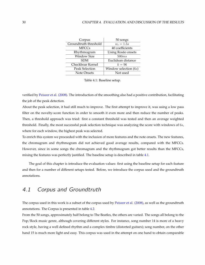
4.1 Method Baseline Setup . . . . . . . . . . . . . . . . . . . . . . . . . . . . . . . . . . . . . . . . . . . 30
4.2 Corpus . . . . . . . . . . . . . . . . . . . . . . . . . . . . . . . . . . . . . . . . . . . . . . . . . . . . 32
4.3 Baseline Average F-measure Results . . . . . . . . . . . . . . . . . . . . . . . . . . . . . . . . . . . . 34
4.4 Average Results - Window Size Experiment . . . . . . . . . . . . . . . . . . . . . . . . . . . . . . . 35
4.5 Average Results - Distance Measure Experiment . . . . . . . . . . . . . . . . . . . . . . . . . . . . 35
4.6 Average Results - Onsets Experiment . . . . . . . . . . . . . . . . . . . . . . . . . . . . . . . . . . . 35
4.7 Best Sum of SDMs Results . . . . . . . . . . . . . . . . . . . . . . . . . . . . . . . . . . . . . . . . . 36
4.8 Best SVD Results . . . . . . . . . . . . . . . . . . . . . . . . . . . . . . . . . . . . . . . . . . . . . . 36
4.9 Best Intersection Results . . . . . . . . . . . . . . . . . . . . . . . . . . . . . . . . . . . . . . . . . . 37
4.10 Average Results - Feature Mixture Experiment . . . . . . . . . . . . . . . . . . . . . . . . . . . . . 37
4.11 Average Results - Feature Mixture Experiment . . . . . . . . . . . . . . . . . . . . . . . . . . . . . 37
4.12 Method Best Setup . . . . . . . . . . . . . . . . . . . . . . . . . . . . . . . . . . . . . . . . . . . . . 38
4.13 Best Result . . . . . . . . . . . . . . . . . . . . . . . . . . . . . . . . . . . . . . . . . . . . . . . . . . 39
4.14 State of the Art Results . . . . . . . . . . . . . . . . . . . . . . . . . . . . . . . . . . . . . . . . . . . 40
4.15 MIREX Boundary recovery results . . . . . . . . . . . . . . . . . . . . . . . . . . . . . . . . . . . . 40
ix

x
Nomenclature
abs Absolute value
AT Automatic generated boundaries
Ck Gaussian tapered checkboard
ds Distance measure function
F F-measure
GT Groundtruth boundary annotations
N Novelty-score function
P Precision
r Correlation coefficient
R Recall
v Feature vector
ws Window size
wt Groundtruth threshold
xi

xii
1Introduction
The expansion of music in digital format due to the growing efficiency of compression algorithms led to the
massification of music consumption. Such a phenomenon led to the creation of a new research field called
musical information retrieval (MIR). Information retrieval (IR) is the science of retrieving from a collection of
items a subset that serves some defined purpose. In this case it is applied to music.
The goal of this chapter is to present the context in which this thesis has been developed, including the moti-
vation for this work, some practical aspects related to automatic audio segmentation and finally a summary of
the work carried out and how it is organized.
1.1 Music - Audio Signal
In an objective and simple way music can be defined as the art of arranging sounds and silences in time.
Any sound can be described as a combination of sine waves, each with its own frequency of vibration, ampli-
tude, and phase. In particular, the sounds produced by musical instruments are the result of the combination
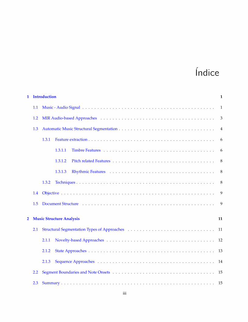
of different frequencies, which are all multiple integers of a fundamental frequency, called harmonics, (figure 1.1).
The perception of this frequency is called pitch, which is one of the characterizing elements of a sound along-
side loudness (related with the amplitude of the signal) and timbre. Typically, humans cannot perceive the
harmonics as separate notes. Instead, a musical note composed of many harmonically related frequencies is
perceived as one sound, where the relative strengths of the individual harmonic frequencies gives the timbre
of that sound.
Considering polyphonic music, sound is composed by various instruments that interact through time,
all together, composing the diverse dimensions of music. The main musical dimensions of interest for music
retrieval are:
Timbre can be simply defined as everything about a sound which is neither loudness nor pitch (Erickson
1975). As an example, it is what is different about the same tone performed in an acoustic guitar and a
flute.
2 CHAPTER 1. INTRODUCTION
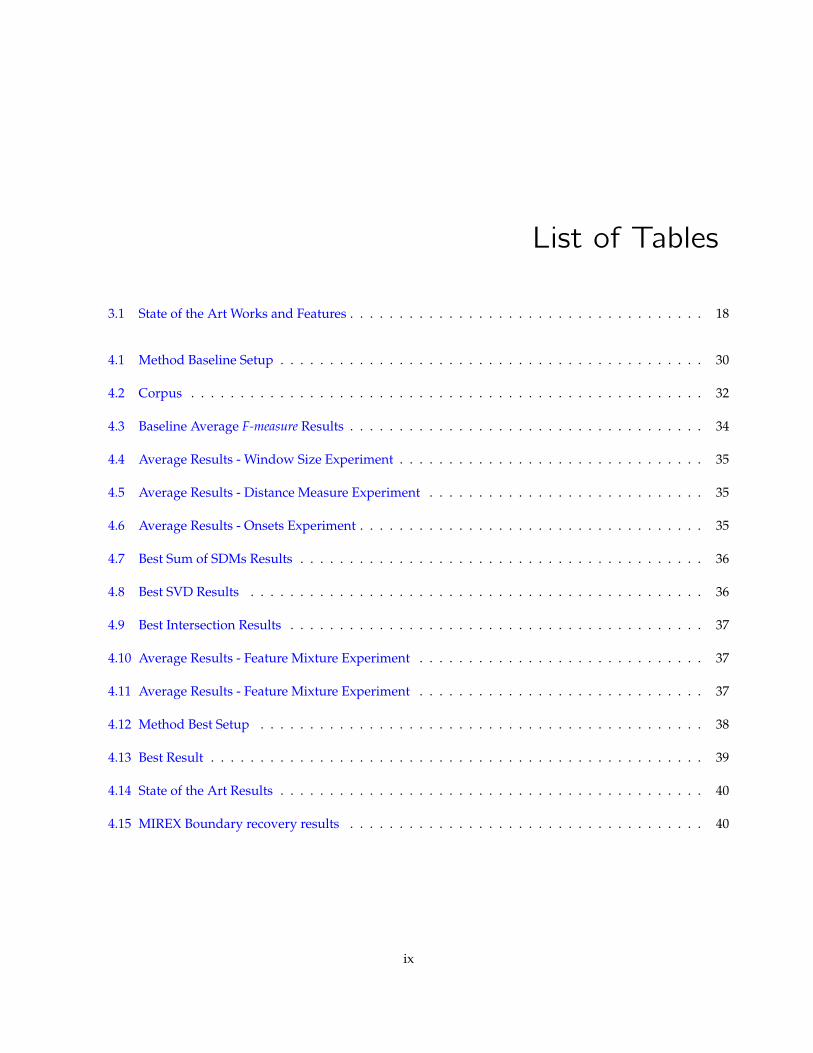
Figure 1.1: The figure presents some periodic audio signals on the left and their frequency counterparts, onthe right. The first signal is a simple sine wave used to tune musical instruments. As can be seen, the subse-quent signals in time present a growing complexity relatively to the sine wave. Their harmonics are the peakspresented on the frequency plot, evident on the violin and flute.
Rhythm is the arrangement of sounds and silences in time. It is related to the periodic repetition of a temporal
pattern of onsets. The perception of rhythm is closely related to the sound onsets alone, so sounds can
be unpitched, as for example the percussion instruments sounds are.
Melody is a linear succession of musical tones which is perceived as a single entity. Usually the tones have
similar timbre and a recognizable pitch within a small frequency range.
Harmony is the conjugation of diverse pitches simultaneously. Harmony can be conveyed by polyphonic
instruments, by a group of monophonic instrument, or may be indirectly implied by the melody.
Structure is on a different level of the previous dimensions, as it covers them all. Structure, or musical form,
relates to the way previous dimensions create determined patterns making structural segments that re-
peat themselves in some way, like the chorus, the verse and so on.
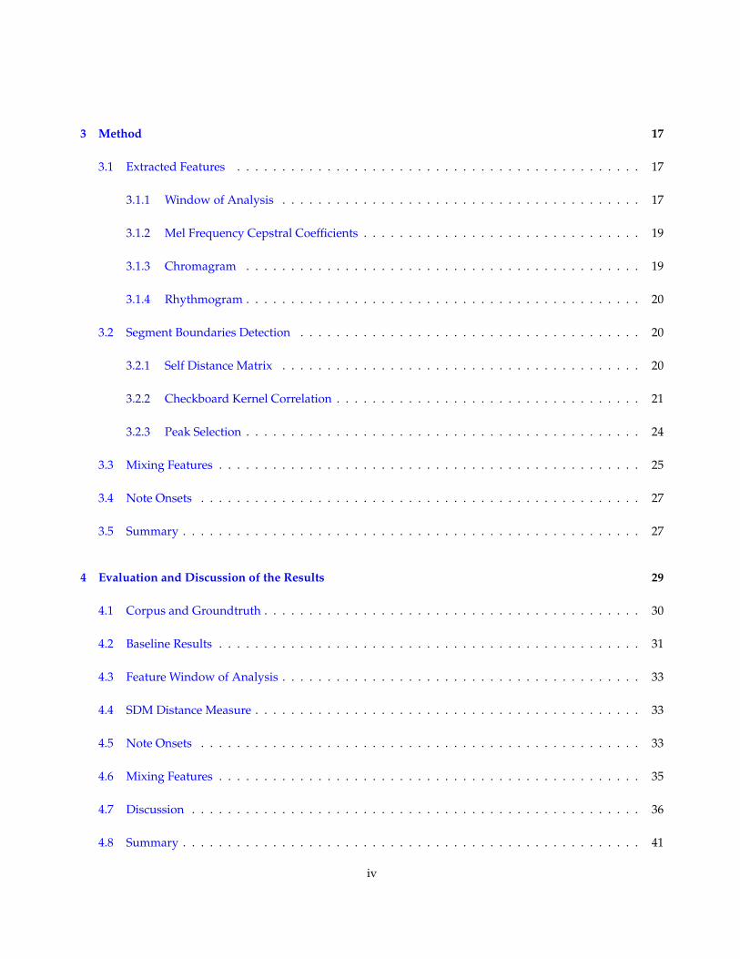
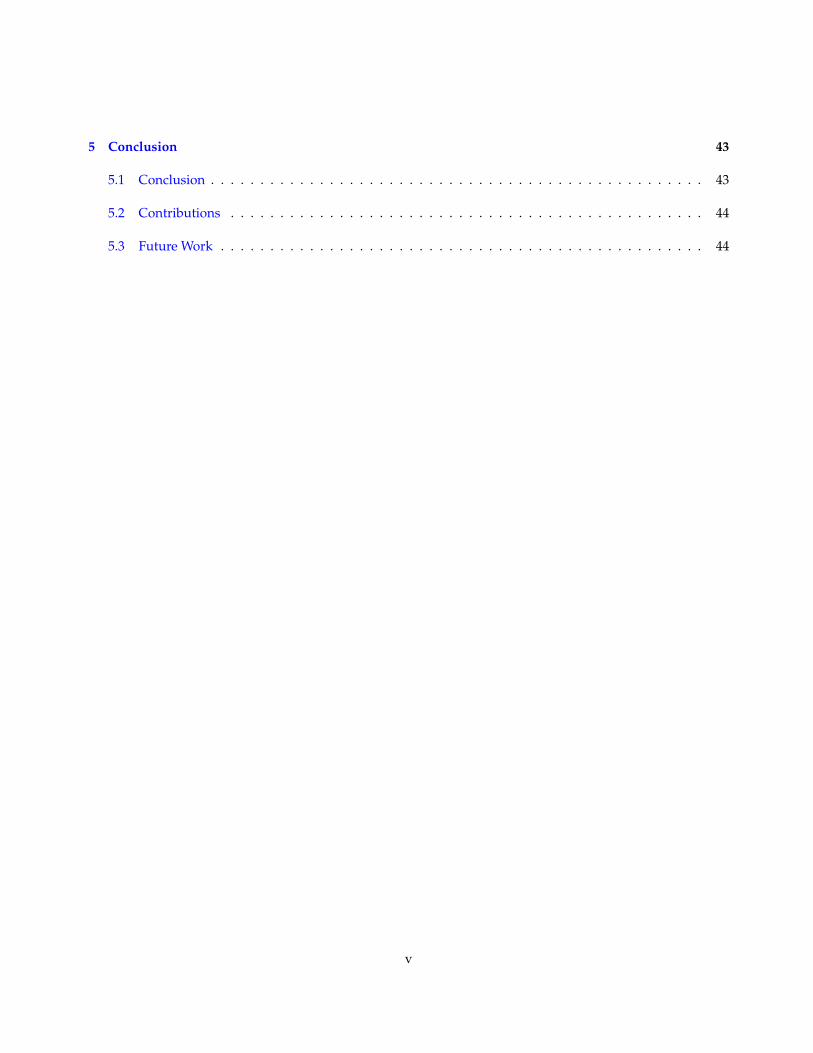
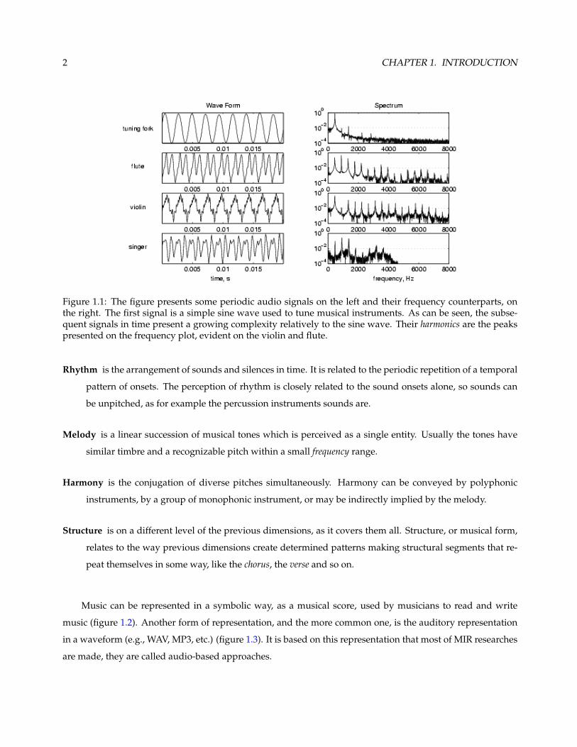
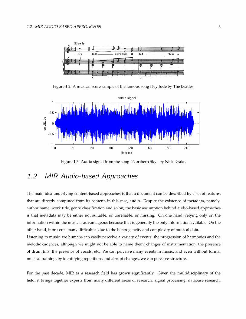
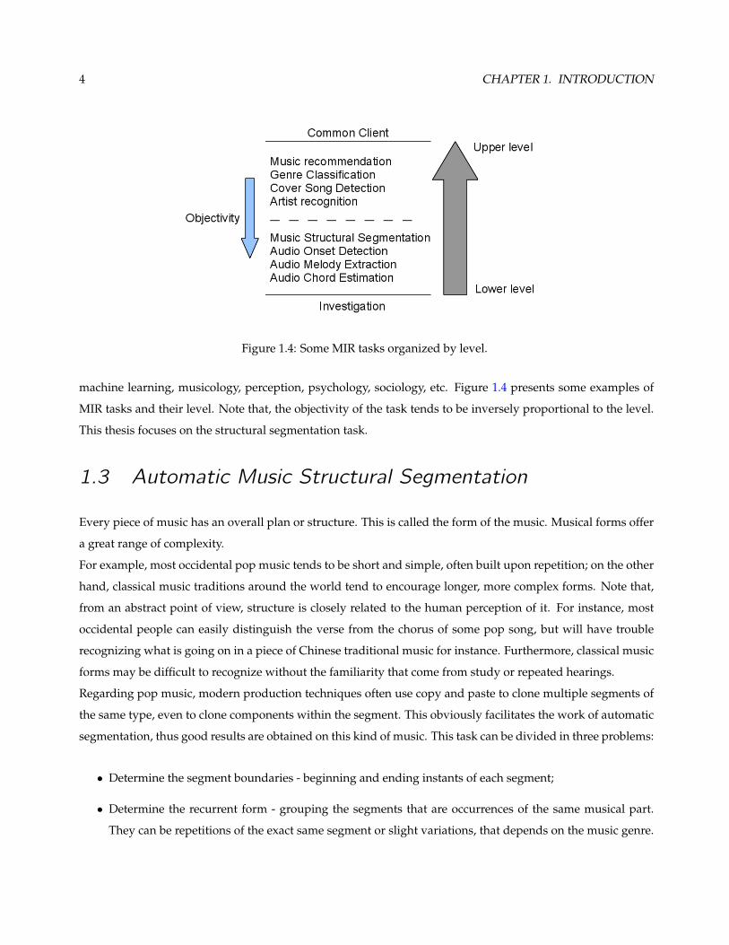
Music can be represented in a symbolic way, as a musical score, used by musicians to read and write
music (figure 1.2). Another form of representation, and the more common one, is the auditory representation
in a waveform (e.g., WAV, MP3, etc.) (figure 1.3). It is based on this representation that most of MIR researches
are made, they are called audio-based approaches.
1.2. MIR AUDIO-BASED APPROACHES 3
Figure 1.2: A musical score sample of the famous song Hey Jude by The Beatles.
Figure 1.3: Audio signal from the song ”Northern Sky” by Nick Drake.
1.2 MIR Audio-based Approaches
The main idea underlying content-based approaches is that a document can be described by a set of features
that are directly computed from its content, in this case, audio. Despite the existence of metadata, namely:
author name, work title, genre classification and so on; the basic assumption behind audio-based approaches
is that metadata may be either not suitable, or unreliable, or missing. On one hand, relying only on the
information within the music is advantageous because that is generally the only information available. On the
other hand, it presents many difficulties due to the heterogeneity and complexity of musical data.
Listening to music, we humans can easily perceive a variety of events: the progression of harmonies and the
melodic cadences, although we might not be able to name them; changes of instrumentation, the presence
of drum fills, the presence of vocals, etc. We can perceive many events in music, and even without formal
musical training, by identifying repetitions and abrupt changes, we can perceive structure.
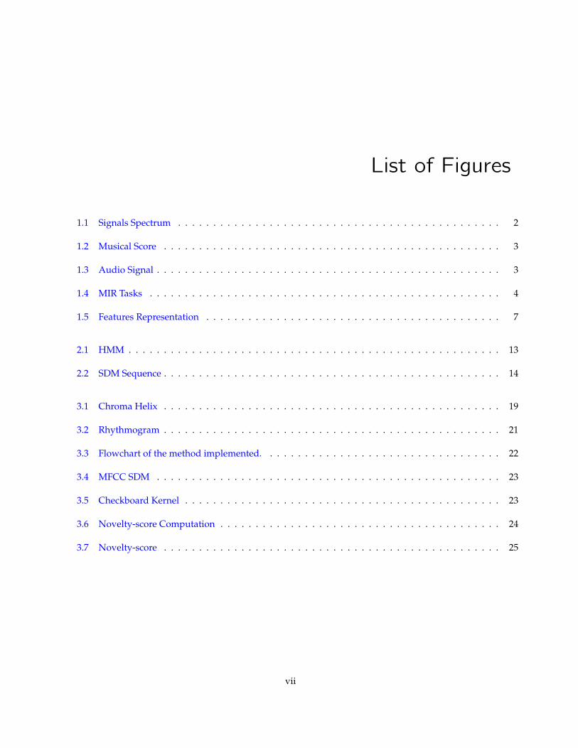
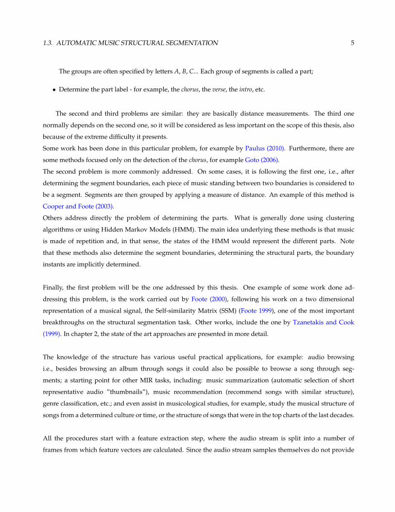
For the past decade, MIR as a research field has grown significantly. Given the multidisciplinary of the
field, it brings together experts from many different areas of research: signal processing, database research,
4 CHAPTER 1. INTRODUCTION
Figure 1.4: Some MIR tasks organized by level.
machine learning, musicology, perception, psychology, sociology, etc. Figure 1.4 presents some examples of
MIR tasks and their level. Note that, the objectivity of the task tends to be inversely proportional to the level.
This thesis focuses on the structural segmentation task.
1.3 Automatic Music Structural Segmentation
Every piece of music has an overall plan or structure. This is called the form of the music. Musical forms offer
a great range of complexity.
For example, most occidental pop music tends to be short and simple, often built upon repetition; on the other
hand, classical music traditions around the world tend to encourage longer, more complex forms. Note that,
from an abstract point of view, structure is closely related to the human perception of it. For instance, most
occidental people can easily distinguish the verse from the chorus of some pop song, but will have trouble
recognizing what is going on in a piece of Chinese traditional music for instance. Furthermore, classical music
forms may be difficult to recognize without the familiarity that come from study or repeated hearings.
Regarding pop music, modern production techniques often use copy and paste to clone multiple segments of
the same type, even to clone components within the segment. This obviously facilitates the work of automatic
segmentation, thus good results are obtained on this kind of music. This task can be divided in three problems:
• Determine the segment boundaries - beginning and ending instants of each segment;
• Determine the recurrent form - grouping the segments that are occurrences of the same musical part.
They can be repetitions of the exact same segment or slight variations, that depends on the music genre.
1.3. AUTOMATIC MUSIC STRUCTURAL SEGMENTATION 5
The groups are often specified by letters A, B, C... Each group of segments is called a part;
• Determine the part label - for example, the chorus, the verse, the intro, etc.
The second and third problems are similar: they are basically distance measurements. The third one
normally depends on the second one, so it will be considered as less important on the scope of this thesis, also
because of the extreme difficulty it presents.
Some work has been done in this particular problem, for example by Paulus (2010). Furthermore, there are
some methods focused only on the detection of the chorus, for example Goto (2006).
The second problem is more commonly addressed. On some cases, it is following the first one, i.e., after
determining the segment boundaries, each piece of music standing between two boundaries is considered to
be a segment. Segments are then grouped by applying a measure of distance. An example of this method is
Cooper and Foote (2003).
Others address directly the problem of determining the parts. What is generally done using clustering
algorithms or using Hidden Markov Models (HMM). The main idea underlying these methods is that music
is made of repetition and, in that sense, the states of the HMM would represent the different parts. Note
that these methods also determine the segment boundaries, determining the structural parts, the boundary
instants are implicitly determined.
Finally, the first problem will be the one addressed by this thesis. One example of some work done ad-
dressing this problem, is the work carried out by Foote (2000), following his work on a two dimensional
representation of a musical signal, the Self-similarity Matrix (SSM) (Foote 1999), one of the most important
breakthroughs on the structural segmentation task. Other works, include the one by Tzanetakis and Cook
(1999). In chapter 2, the state of the art approaches are presented in more detail.
The knowledge of the structure has various useful practical applications, for example: audio browsing
i.e., besides browsing an album through songs it could also be possible to browse a song through seg-
ments; a starting point for other MIR tasks, including: music summarization (automatic selection of short
representative audio ”thumbnails”), music recommendation (recommend songs with similar structure),
genre classification, etc.; and even assist in musicological studies, for example, study the musical structure of
songs from a determined culture or time, or the structure of songs that were in the top charts of the last decades.
All the procedures start with a feature extraction step, where the audio stream is split into a number of
frames from which feature vectors are calculated. Since the audio stream samples themselves do not provide
6 CHAPTER 1. INTRODUCTION
relevant information, feature extraction is essential. And even more essential is to understand the meaning
of the extracted features, i.e. what they represent regarding the musical dimensions. The subsequent steps,
depend on the procedure and on the goals that are to be reached (summarization, chorus detection, segment
boundaries detection, etc.), however, they are limited to the extracted features and what they represent. So the
feature extraction step plays a central role in any MIR procedure.
1.3.1 Feature extraction
Feature extraction is essential for any music information retrieval system. In particular, when detecting seg-
ment boundaries. In general, humans can easily perceive segment boundaries in popular music that is familiar
to them. But what information contained in a musical signal is important to perceive that event?
According to Bruderer et al experiments on humans perception of structural boundaries in popular mu-
sic (Bruderer et al. 2006); ”global structure” (repetition, break), ”change in timbre”, ”change in level” and
”change in rhythm”, represent the main perceptual cues responsible for the perceiving of boundaries in music.
Therefore, in order to optimize the detection of such boundaries, extracted features shall roughly represent the
referred perceptual cues.
Considering the perceptual cues and the presented musical dimensions, the musical signal is generally
summarized in three dimensions: the timbre, the tonal part (pitch related, harmony and melody) and the
rhythm. The features used in our method are presented in more detail in chapter 3.
1.3.1.1 Timbre Features
Perceptually, timbre is one of the most important dimensions in a piece of music. Its importance relatively
other musical dimensions can be easily understood by the fact that anyone can recognize familiar instruments,
even without conscious thought, and people are able to do it with much less effort and much more accuracy
than for recognizing harmonies or scales.
As determined by Terasawa et al. (2005), Mel-frequency cepstral coefficients (MFCC) are a good model
for the perceptual timbre space. MFCC is well known as a front-end for speech recognition systems. The first
part of figure 1.5 represents a 40 dimensional MFCC vector over time.
In addition to the use of MFCCs, in order to complete the timbre information of the musical signal, compu-
tation of: spectral centroid, spectral spread and spectral slope can be also useful (Kaiser and Sikora 2010). As an
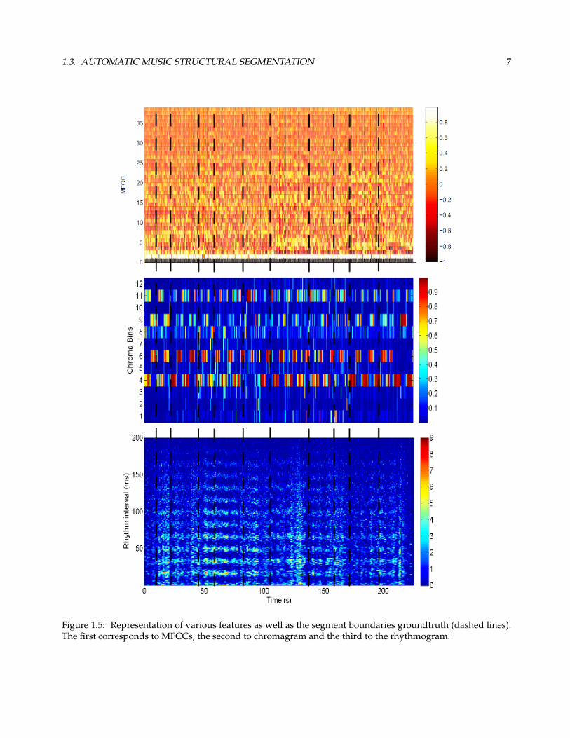
1.3. AUTOMATIC MUSIC STRUCTURAL SEGMENTATION 7
Figure 1.5: Representation of various features as well as the segment boundaries groundtruth (dashed lines).The first corresponds to MFCCs, the second to chromagram and the third to the rhythmogram.
8 CHAPTER 1. INTRODUCTION
alternative to the use of MFCCs, Levy and Sandler (2008) uses AudioSpactrumEnvelope, AudioSpectrumProjection
and SoundModel descriptors of the MPEG-7 standard.
Other alternative feature, include the Perceptual Linear Prediction (PLP) (Hermansky 1990), used by
Jensen (2007).
1.3.1.2 Pitch related Features
Pitch, upon which harmonic and melodic sequences are built, represents an important musical dimension.
One example of its importance to the human perception, are the music covers. Music covers usually preserve
harmony and melody while using a different set of musical instruments, thus altering the timbre information
of the song. However, they are usually accurately recognized by people.
In the context of music structural segmentation, chroma features represent the most powerful represen-
tation for describing harmonic information (Muller 2007). The most important advantage of chroma features
is their robustness to changes in timbre. A similar feature is the Pitch Class Profile coefficients (PCP) (Gomez
2006), used by Shiu et al. (2006).
1.3.1.3 Rhythmic Features
The rhythmic features are among the less used in the task of music structural segmentation. Considering the
perceptual cue identified by Bruderer et al. study, ”change in rhythm” . In fact, Paulus and Klapuri (2008) noted
that the use of rhythmic information in addition to timbre and harmonic features provide useful information
to structure analysis.
The rhythmic content of a musical signal can be described with a rhythmogram as introduced by Jensen
(2004) (third part of figure 1.5). It is comparable to a spectrogram, but instead of representing the frequency
spectrum of the signal, it represents the rhythmic content.
1.3.2 Techniques
Some techniques were already referred in the beginning of this section, they are presented in more detail in
chapter 2:
Self Distance Matrix The Self Distance Matrix (SDM) compares the feature vectors with each other, using
some determined distance measure (for example, the euclidean) (Foote 1999).
1.4. OBJECTIVE 9
Hidden Markov Models The use of an HMM to represent music, assumes that each state represents some
musical information, thus defining a musical alphabet, where each state represents a letter.
Clustering The idea underlying the use of clusters to represent music is that different segments are repre-
sented by different clusters.
Time difference Using the time differential of the feature vector large differences would indicate sudden tran-
sitions, thus a possible segment boundaries boundaries.
Cost Function The cost function determines the cost of a determined segment, so that, segments where the
composing frames have a high degree of self similarity have a low cost.
1.4 Objective
The goal of this thesis is to perform structural segmentation on audio stream files, that is, to identify the
instants of segment change, boundaries between segments. The computed boundaries will be then compared
with manually noted ones in order to evaluated their quality.
1.5 Document Structure
After presenting the context in which this thesis has been developed, including the motivation for this work
and some practical aspects related to automatic audio segmentation. The remaining of this document is orga-
nized as follows:
Chapter 2 introduces the state of the art approaches.
Chapter 3 introduces the used features, followed by the presentation of the implemented method and each
used tool.
Chapter 4 introduces the final results discussion and a comparison with the state of art ones.
Chapter 5 introduces the conclusions and future work.

10 CHAPTER 1. INTRODUCTION
2Music Structure Analysis
Music is structured, generally respecting some rules that vary regarding the genre of music. Music can be
divided into many genres in many different ways. And each genre of music can also be divided in a variety
of styles. For instance, the Pop/Rock genre includes over 50 different styles1, and most of them are extremely
different (for example: Death Metal and Country Rock). Then, even if there is controversy on the way music
genres are divided, the diversity of sounds in different genres is unquestionable. In that sense, achieving the
capability to adapt to such a variety of sounds presents the major difficulty for the automatic segmentation
approaches.
The goal of this chapter is to introduce the state of the art approaches to the problem of structural segmentation
in music. They are organized in three sets as proposed by Paulus et al. (2010): novelty-based approaches,
state approaches and sequence approaches. Additionally, it will discuss the relation between the segment
boundaries and the note onsets.
2.1 Structural Segmentation Types of Approaches
The various techniques used to solve the structural segmentation problem so far can be grouped according to
their paradigm. Peeters (2004) considered dividing the approaches into two sets: ”sequence” approaches and
”state” approaches. The ”sequence” approaches consider that there are sequences of events that are repeated
several times in a given music. The ”state” approaches consider the musical audio signal to be a succession
of states, where each state produces some part of the signal. Paulus et al. (2010) on the other hand, suggested
dividing the methods into three main sets: novelty-based approaches, homogeneity-based approaches and
repetition-based approaches. In fact, the homogeneity-based approaches are basically the same as the ”state”
approaches defined by Peeters, and the repetition-based approaches are the ”sequence” approaches. The third
set proposed by Paulus, novelty-based approach, can be seen as a front-end for one of the other approaches or
both. The goal of this section is to introduce each one of the three sets of approaches, as well as the state of the
1http://www.allmusic.com/explore/genre/poprock-d20
12 CHAPTER 2. MUSIC STRUCTURE ANALYSIS
art methods referred to each. Starting with the novelty-based approaches, followed by the state approaches
and finally the sequence approaches.
2.1.1 Novelty-based Approaches
The goal of the novelty-based approaches is to locate instants where changes occur in a song, usually referred
to as segment boundaries. Knowing those, segments can be defined between them.
The most common way of doing so is using a Self-Distance Matrix (SDM). The SDM is computed as follows:
SDM(i, j) = ds(vi, vj) i, j = 1, ..., n (2.1)
Where ds represents a distance measure (for example, Euclidean distance), v represents a feature vector
and i and j are the frame numbers, where a frame is the smallest piece of music used. Using a checkboard
kernel (figure 3.5) to be correlated along the diagonal of the SDM yields a novelty-score function. The peaks
of the novelty score represent candidate boundaries between segments. This method was first introduced by
Foote (2000). More about this method is introduced in chapter 3.
Other method to detect boundaries was proposed by Tzanetakis and Cook (1999), by using the time dif-
ferential of the feature vector, defined as the Mahalanobis distance:
∇i = ((vi − vi−1)T (∑
)−1(vi − vi−1)) (2.2)
where∑
is an estimate of the feature covariance matrix, calculated from the training data, and i is the
frame number. This measure is related to the Euclidean distance but takes into account the variance and
correlations among features. Large differences would indicate sudden transitions, thus a possible boundary.
More recently, Jensen (2007) proposed a method where boundaries are detected using a cost function. This
cost function determines the cost of a determined segment, so that, segments where the composing frames have
a high degree of self similarity have a low cost.
2.1. STRUCTURAL SEGMENTATION TYPES OF APPROACHES 13
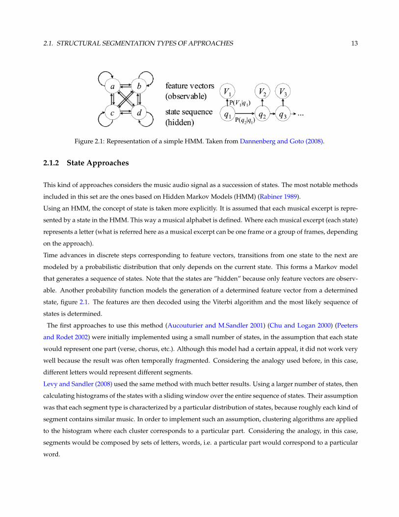
Figure 2.1: Representation of a simple HMM. Taken from Dannenberg and Goto (2008).
2.1.2 State Approaches
This kind of approaches considers the music audio signal as a succession of states. The most notable methods
included in this set are the ones based on Hidden Markov Models (HMM) (Rabiner 1989).
Using an HMM, the concept of state is taken more explicitly. It is assumed that each musical excerpt is repre-
sented by a state in the HMM. This way a musical alphabet is defined. Where each musical excerpt (each state)
represents a letter (what is referred here as a musical excerpt can be one frame or a group of frames, depending
on the approach).
Time advances in discrete steps corresponding to feature vectors, transitions from one state to the next are
modeled by a probabilistic distribution that only depends on the current state. This forms a Markov model
that generates a sequence of states. Note that the states are ”hidden” because only feature vectors are observ-
able. Another probability function models the generation of a determined feature vector from a determined
state, figure 2.1. The features are then decoded using the Viterbi algorithm and the most likely sequence of
states is determined.
The first approaches to use this method (Aucouturier and M.Sandler 2001) (Chu and Logan 2000) (Peeters
and Rodet 2002) were initially implemented using a small number of states, in the assumption that each state
would represent one part (verse, chorus, etc.). Although this model had a certain appeal, it did not work very
well because the result was often temporally fragmented. Considering the analogy used before, in this case,
different letters would represent different segments.
Levy and Sandler (2008) used the same method with much better results. Using a larger number of states, then
calculating histograms of the states with a sliding window over the entire sequence of states. Their assumption
was that each segment type is characterized by a particular distribution of states, because roughly each kind of
segment contains similar music. In order to implement such an assumption, clustering algorithms are applied
to the histogram where each cluster corresponds to a particular part. Considering the analogy, in this case,
segments would be composed by sets of letters, words, i.e. a particular part would correspond to a particular
word.
14 CHAPTER 2. MUSIC STRUCTURE ANALYSIS
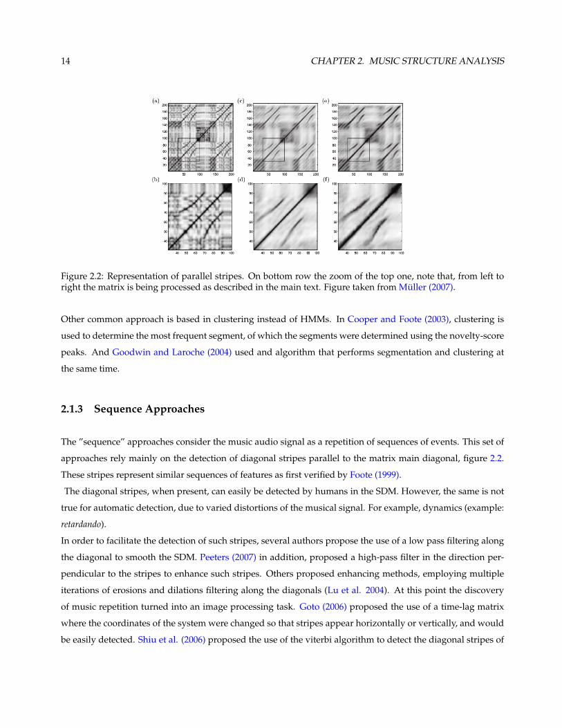
Figure 2.2: Representation of parallel stripes. On bottom row the zoom of the top one, note that, from left toright the matrix is being processed as described in the main text. Figure taken from Muller (2007).
Other common approach is based in clustering instead of HMMs. In Cooper and Foote (2003), clustering is
used to determine the most frequent segment, of which the segments were determined using the novelty-score
peaks. And Goodwin and Laroche (2004) used and algorithm that performs segmentation and clustering at
the same time.
2.1.3 Sequence Approaches
The ”sequence” approaches consider the music audio signal as a repetition of sequences of events. This set of
approaches rely mainly on the detection of diagonal stripes parallel to the matrix main diagonal, figure 2.2.
These stripes represent similar sequences of features as first verified by Foote (1999).
The diagonal stripes, when present, can easily be detected by humans in the SDM. However, the same is not
true for automatic detection, due to varied distortions of the musical signal. For example, dynamics (example:
retardando).
In order to facilitate the detection of such stripes, several authors propose the use of a low pass filtering along
the diagonal to smooth the SDM. Peeters (2007) in addition, proposed a high-pass filter in the direction per-
pendicular to the stripes to enhance such stripes. Others proposed enhancing methods, employing multiple
iterations of erosions and dilations filtering along the diagonals (Lu et al. 2004). At this point the discovery
of music repetition turned into an image processing task. Goto (2006) proposed the use of a time-lag matrix
where the coordinates of the system were changed so that stripes appear horizontally or vertically, and would
be easily detected. Shiu et al. (2006) proposed the use of the viterbi algorithm to detect the diagonal stripes of
2.2. SEGMENT BOUNDARIES AND NOTE ONSETS 15
musical parts that present a weaker similarity value, for example verses.
These approaches somehow fail in a basic assumption that the stripes are parallel the main diagonal. Further-
more, although the detection of sequence repetition represents a great improvement to the musical structure
analysis, it is not usually enough to represent the whole higher level structural segmentation, as it requires a
part to occur at least twice to be found. Accordingly the combination of ”state” approaches with ”sequence”
approaches appear to be the most reasonable. A good example of the combination of both approaches is the
work done by Paulus and Klapuri (2009).
2.2 Segment Boundaries and Note Onsets
The note onsets are defined as the start of a musical note, not only pitched notes but also unpitched ones,
rhythmic notes. In monophonic music a note onset is well defined as well as its duration, however, in poly-
phonic music, note onsets of various instruments overlap. This makes them more difficult to identify, both
automatically and perceptually. A variety of methods to detect the note onsets are presented by Rosao and
Ribeiro (2011).
Considering the detection of segment boundaries task, it is of our belief that the note onsets can be used to
validate the segment boundaries. The assumption is that any segment is defined between note onsets, then
any segment must start in a note onset. In that sense, the note onsets are seen as the events that ”trigger” the
segment change. Not only the segment change but every other event in music. In the extreme, without note
onsets there is absence of sound.
2.3 Summary
In this chapter the state of the art approaches were introduced according to the division proposed by Paulus
et al. (2010): novelty-based approaches, state approaches and sequence approaches. The first set is focused on
the detection of segment boundaries and is generally used as front-end for one of the other approaches. The
second set, considers the musical audio signal to be a succession of states, where each state produces some
part of the signal. The last set, considers that there are sequences of events repeated several times in a given
music. To finalize the chapter, we considered the note onsets to be events that ”trigger” the segment change.

16 CHAPTER 2. MUSIC STRUCTURE ANALYSIS
3Method
Considering the introduced sets of methods, the implemented method belongs to the novelty-based ap-
proaches. It is focused on determining the segment boundaries.
The goal of this chapter is to introduce the method developed aiming to solve the problem of segmentation of
audio music streams, describing each used tool. It starts by considering the features collected from the audio
stream and how they were mixed, followed by the introduction of the actual method.
3.1 Extracted Features
The extraction of features is a very important step in any MIR system. Table 3.1 shows the features used in
some structural segmentation works. In our case the features extracted are an attempt to represent the main
three musical dimensions: timbre, tonal (harmony and melody) and rhythmic.
In this section, we introduce the extracted features and their mixture, before, we consider the windows of
analysis used to collect those features.
3.1.1 Window of Analysis
The audio stream is first downsampled to 22050Hz, since this number of samples is enough. Considering
those samples, they are then grouped in windows or frames.
In music structure segmentation to compare frames with each other is a usual task, as it is evident in the SDM.
Such a task can represent heavy computation depending on the number of frames used. Generally, larger frame
length are used (0.1−1s), compared with most of the audio content analysis (0.01−0.1s). This fact reduces the
number of frames in a song, thus reducing the SDM size. Moreover, larger frame length allows a larger tem-
poral resolution which according to Peeter represents something musically more meaningful (Peeters 2004).
Some proposed methods unlike using fixed length frames tend to use variable ones. This has two benefits:
tempo invariance, which means that some melody, for example, that has some tempo fluctuation relatively
the same pitch progression melody, can be successfully match; sharper feature differences, preventing sound
18 CHAPTER 3. METHOD
Authors Task FeaturesGoto (2006) Chorus Detection ChromaJensen (2007) Music Structure Perceptual Linear Prediction
(PLP), Chroma and Rhythmo-gram
Kaiser and Sikora (2010) Music Structure 13 MFCCs, spectral centroid,spectral slope and spectralspread
Levy and Sandler (2008) Music Structural Segmentation AudioSpectrumEnvelope, Au-dioSpectrumProjection, andSoundModel descriptors of theMPEG-7 standard
Paulus and Klapuri (2009) Music Structural Segmentation 12 MFCCs (excluding the 0th),Chroma and Rhythmogram
Peeters (2007) Music Structural Segmentation 13 MFCCs (excluding the 0th),12 Spectral Contrast coefficientsand Pitch Class Profile coeffi-cients
Peiszer et al. (2008) Music Structural Segmentation 40 MFCCsShiu et al. (2006) Similar Segment Identification Pitch Class Profile coefficientsTurnbull and Lanckriet (2007) Music Structural Segmentation MFCCs and Chroma
Table 3.1: Compilation of works and features used.
events respective features from spreading to other frames. Peiszer et al. (2008) for example, used the note
onsets to set out window sizes.
In our case, in order to accomplish sharper feature difference, the size of the windows are determined de-
pending on the bpm. The bpm are determined using the function mirtempo() from MIRtoolbox (Lartillot 2011),
which estimates the tempo by detecting periodicities from the onset detection curve. In this case the onsets are
determined using the function mironsets() also from the MIRtoolbox. The mirtempo() function is quite accurate.
It is made the assumption that the tempo in pop music is constant. The window size is determined as follows:
ws =1
2.bpm60
(3.1)
This yields window sizes between 0.15s and 0.3s, which is equivalent to bpm between 100 and 200, depending
on the song. We used no overlapping of windows, except for the rhythmogram.
The impact of using variable window size compared to fixed is discussed with actual evaluation values in the
next chapter.
3.1. EXTRACTED FEATURES 19
Figure 3.1: Pitch represented by two dimensions: height, moving vertically in octaves, and chroma, or pitchclass determining the rotation position within the helix. Taken from Gomez (2006).
3.1.2 Mel Frequency Cepstral Coefficients
The MFCCs are extensively used to represent the timbre in music. We used 40 MFCCs calculated using a
filter bank composed by linear and logarithmic filters to model loudness compression, in order to simulate the
characteristics of the human auditory system. The coefficients are obtained by taking the discrete cosine (DCT)
of the log-power spectrum on the Mel-frequency scale.
Most of the authors do not use more then 20 coefficients. However, some tests were made with 40 coefficients
and final results show that the increase of coefficients has a significant influence (around 5% in our case). This
was also verified by Peiszer et al. (2008), as well as Santos (2010), who also used 40 MFCC. The first part of
figure 1.5 represents a 40 dimensional MFCC vector over time.
3.1.3 Chromagram
The chroma refers to the 12 traditional pitch classes (the 12 semitones) {C, C#, D, ... , A#, B}. As pitch repeats
itself every octaves (12 semitones), a pitch class is defined to be the set of all pitches that share the same
chroma. This is represented in figure 3.1. For example, the pitch class corresponding to the chroma F is the set
{..., F0, F1, F2,...}, where 0, 1 and 2 represent the pitch F of each octave. Therefore, the chroma representation
is a 12 dimensional vector, where each dimension is the respective chroma of the signal. Figure 1.5 shows a
20 CHAPTER 3. METHOD
chromagram, the chroma represented in time.
We used Muller and Ewert (2011) method to extract the chroma features. First, the pitch values are determined
using a 88 filter centered in each pitch, from A0 to C8. The chroma vector is then calculated simply by adding
pitches that correspond to the same chroma.
3.1.4 Rhythmogram
The rhythmogram was first presented by Jensen (2004). It is computed by determining the autocorrelation of
the note onsets on intervals of 2s, using a millisecond scale, what produces o vector of dimension 200, figure
3.2. Unlike the other two features extracted, the rhythmogram is calculated using a window of analysis of
2s and a hop size of ws. This way, the rhythmogram will have the same number of samples per song as the
MFCCs and the chromagram.
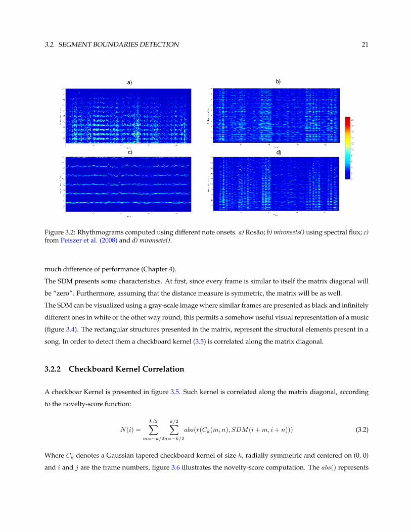
We used 4 different onsets: one taken from Peiszer et al. (2008), which was taken from a beat tracker. Other
by Rosao (2011), based on the Spectral Flux (Bello et al. 2005). And the others using MIRToolbox function
mironsets() (Lartillot 2011): one using the envelope of the signal and the other using the Spectral Flux as well.
The first onsets are very few compared with the other three, this suggest that there must have been some selec-
tion. That fact is adverse to the usefulness of the rhythmogram. As shown in figure 3.2 (c)), the rhythmogram
presents too few information. On the other hand the other note onsets, figure 3.2 (a), b) and d)), convey much
more information. This is reflected on the final results as it will be shown in the next chapter.
3.2 Segment Boundaries Detection
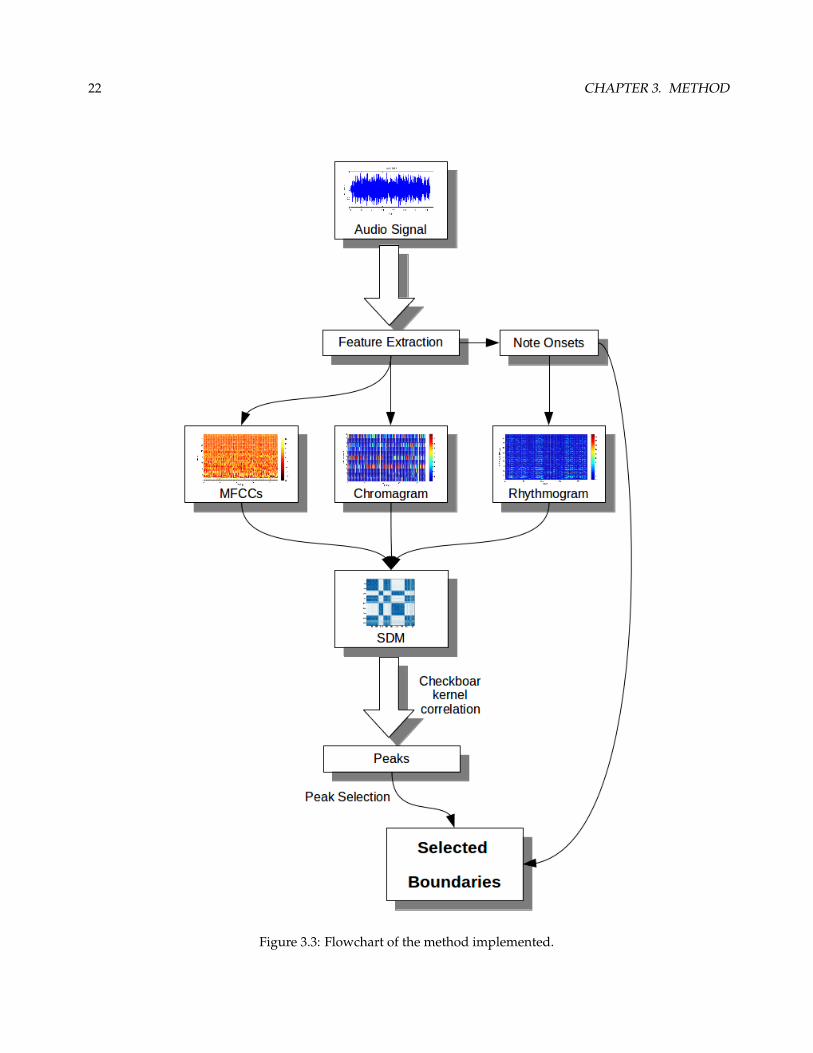
In this section the algorithm is presented. Figure 3.3 represents a flowchart of the implemented method using
Matlab. The used method is based on the approach by Foote (2000), where he first introduced the novelty-score
function. Firstly, the SDM matrix is computed then a novelty-score function is calculated from it and finally
the peaks of such function are determined as candidates for segment boundaries.
Following, each of the steps of the algorithm are presented.
3.2.1 Self Distance Matrix
The SDM is determined by 2.1. The distance measure used was the Manhattan distance measures. As it is
known to perform well when dealing with high dimensionality data (Aggarwal et al. 2001), which is the case.
But the fact is, that experiences made with the Euclidean and the Cosine distance showed that there is not
3.2. SEGMENT BOUNDARIES DETECTION 21
Figure 3.2: Rhythmograms computed using different note onsets. a) Rosao; b) mironsets() using spectral flux; c)from Peiszer et al. (2008) and d) mironsets().
much difference of performance (Chapter 4).
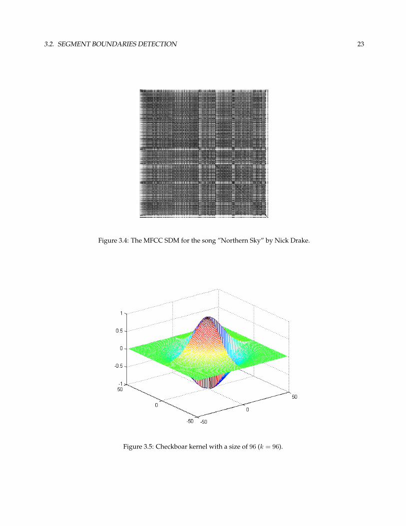
The SDM presents some characteristics. At first, since every frame is similar to itself the matrix diagonal will
be “zero”. Furthermore, assuming that the distance measure is symmetric, the matrix will be as well.
The SDM can be visualized using a gray-scale image where similar frames are presented as black and infinitely
different ones in white or the other way round, this permits a somehow useful visual representation of a music
(figure 3.4). The rectangular structures presented in the matrix, represent the structural elements present in a
song. In order to detect them a checkboard kernel (3.5) is correlated along the matrix diagonal.
3.2.2 Checkboard Kernel Correlation
A checkboar Kernel is presented in figure 3.5. Such kernel is correlated along the matrix diagonal, according
to the novelty-score function:
N(i) =
k/2∑m=−k/2
k/2∑n=−k/2
abs(r(Ck(m,n), SDM(i+m, i+ n))) (3.2)
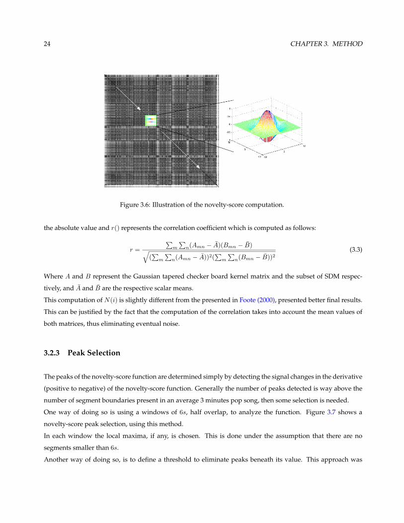
Where Ck denotes a Gaussian tapered checkboard kernel of size k, radially symmetric and centered on (0, 0)
and i and j are the frame numbers, figure 3.6 illustrates the novelty-score computation. The abs() represents
22 CHAPTER 3. METHOD
Figure 3.3: Flowchart of the method implemented.
3.2. SEGMENT BOUNDARIES DETECTION 23
Figure 3.4: The MFCC SDM for the song ”Northern Sky” by Nick Drake.
Figure 3.5: Checkboar kernel with a size of 96 (k = 96).
24 CHAPTER 3. METHOD
Figure 3.6: Illustration of the novelty-score computation.
the absolute value and r() represents the correlation coefficient which is computed as follows:
r =
∑m
∑n(Amn − A)(Bmn − B)√
(∑
m
∑n(Amn − A))2(
∑m
∑n(Bmn − B))2
(3.3)
Where A and B represent the Gaussian tapered checker board kernel matrix and the subset of SDM respec-
tively, and A and B are the respective scalar means.
This computation of N(i) is slightly different from the presented in Foote (2000), presented better final results.
This can be justified by the fact that the computation of the correlation takes into account the mean values of
both matrices, thus eliminating eventual noise.
3.2.3 Peak Selection
The peaks of the novelty-score function are determined simply by detecting the signal changes in the derivative
(positive to negative) of the novelty-score function. Generally the number of peaks detected is way above the
number of segment boundaries present in an average 3 minutes pop song, then some selection is needed.
One way of doing so is using a windows of 6s, half overlap, to analyze the function. Figure 3.7 shows a
novelty-score peak selection, using this method.
In each window the local maxima, if any, is chosen. This is done under the assumption that there are no
segments smaller than 6s.
Another way of doing so, is to define a threshold to eliminate peaks beneath its value. This approach was
3.3. MIXING FEATURES 25
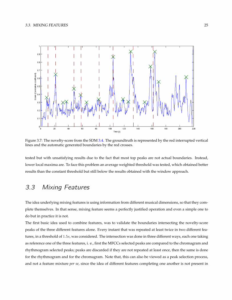
Figure 3.7: The novelty-score from the SDM 3.4. The groundtruth is represented by the red interrupted verticallines and the automatic generated boundaries by the red crosses.
tested but with unsatisfying results due to the fact that most top peaks are not actual boundaries. Instead,
lower local maxima are. To face this problem an average weighted threshold was tested, which obtained better
results than the constant threshold but still below the results obtained with the window approach.
3.3 Mixing Features
The idea underlying mixing features is using information from different musical dimensions, so that they com-
plete themselves. In that sense, mixing feature seems a perfectly justified operation and even a simple one to
do but in practice it is not.
The first basic idea used to combine features, was to validate the boundaries intersecting the novelty-score
peaks of the three different features alone. Every instant that was repeated at least twice in two different fea-
tures, in a threshold of 1.5s, was considered. The intersection was done in three different ways, each one taking
as reference one of the three features, i. e., first the MFCCs selected peaks are compared to the chromagram and
rhythmogram selected peaks; peaks are discarded if they are not repeated at least once, then the same is done
for the rhythmogram and for the chromagram. Note that, this can also be viewed as a peak selection process,
and not a feature mixture per se, since the idea of different features completing one another is not present in
26 CHAPTER 3. METHOD
this approach.
The second idea was to sum the SDMs before the computation of the novelty-score function, as follows:
SDM(M +R) = αSDM(MFCC) + SDM(Rhythmogram) (3.4)
SDM(C +R) = βSDM(Chroma) + SDM(Rhythmogram) (3.5)
SDM(M + C) = SDM(MFCC) + σSDM(Chroma) (3.6)
SDM(M + C +R) = αSDM(MFCC) + βSDM(Chroma) + SDM(Rhythmogram) (3.7)
Where, the SDMs respective features are represented in brackets. M, C and R stand for, MFCC, Chromagram
and Rhythmogram respectively. The coefficients alpha, beta and sigma are computed as follows:
α =mean(SDM(Rhythmogram))
mean(SDM(MFCC); (3.8)
β =mean(SDM(Rhythmogram))
mean(SDM(Chroma); (3.9)
σ =mean(SDM(MFCC))
mean(SDM(Chroma); (3.10)
Where, the operation mean() determines the mean value of the matrix. The purpose of it is balancing the
factors of the sum, trying to give the same weight to each one.
Finally, the third idea was to use a dimensionality reduce method on the concatenated feature vector, combin-
ing features in groups of two and three. This created new feature vectors, then used to compute the SDM and
the remainder of the method. To that end, the Singular Value Decomposition (SVD) method was used.
The SVD is based on a theorem from linear algebra which says that a rectangular matrix M (which in this case
represents the feature vectors) can be broken down into the product of three matrices: an orthogonal matrix U ,
a diagonal matrix S, and the transpose of an orthogonal matrix V . The decomposition is usually presented as:
Mmn = UmmSmnVTnn (3.11)
According to the diagonal of S, which present a descending curve representing the descending representation
of each feature vector, the first n vectors from V Tnn are used, meaning that the ones that are left unused are
useless or even adverse (noise) for further computations.
The results for each hypothesis are presented and discussed in the next chapter.
3.4. NOTE ONSETS 27
3.4 Note Onsets
The note onsets are used in the algorithm in order to validate the selected peaks from the novelty-score. This
is done by swapping each novelty-score peak by the note onset closer to it.
This operation could also be considered a peak selection operation, instead of the used ”window” approach,
applying this operation would eventually mean that many peaks would be represented by the same onset.
Then, the number of peaks will be reduced. However, this approach produces too many peaks still. An
attempt was made to reduce the number of onsets first, using the same window approach, so that a lesser
number of peaks was produced. However, results were not satisfying. The note onsets are then used in the
assumption that they will correct in time the novelty-score peaks selected by the ”windows” approach.
The onsets used are presented in 3.1.4. The final result for each one is presented in the next chapter.
3.5 Summary
In this chapter the method implemented was introduced. We used three features: the MFCC, the Chromagram
and the Rhythmogram. Each representing the timbre, the tonal information and the rhythm respectively. This
features were used in a novelty-based approach. Where segment boundaries are determined based on the
novelty-score function, determined from the correlation of a checkboard kernel along the SDM diagonal. The
peaks of such function are candidates, which are then selected. The features were also combined in three
different ways. The final boundaries are then adjusted to a grid of note onsets.
T

28 CHAPTER 3. METHOD
4Evaluation and Discussion
of the Results
In order to evaluate the automatic segmentation algorithm, a manual groundtruth segmentation has to be
done, and a measure of the accuracy computed.
According to the most used approach, e.g. Peiszer et al. (2008), the precision (P ), recall (R) and F-measure (F ),
are calculated to evaluate the success of the method. They are calculated as follows:
P =|AT ∩wt
GT ||GT |
R =|AT ∩wt
GT ||AT |
(4.1)
Where, GT and AT denote the groundtruth boundaries and the automatic generated boundaries respectively.
w determines how far two boundaries can be apart but still count as one (we used wt = 1.5s). Finally, F is the
harmonic mean of P and R.
We begin by describing the first implemented approach, the baseline. The MFCCs were the first feature
to be used. At first, only 13 coefficients were extracted, using a fixed length window (500ms). The SDM was
computed using the Euclidean distance and the novelty-score was computed using a checkboard kernel with
no radial smoothing, only a matrix of zeros and ones sized 128. The obtained function peaks were selected by
choosing the first 15 peaks according to their coordinate value.
After this start we knew that results could be improved only by changing the parameters for these tools.
Tests were first made using different distance measures to compute the SDM. Since there were available a
series of distance measure for Matlab function pdist(), we tested some. The best results were obtained with the
Cosine distance, the Manhattan distance (or City Block) and the Euclidean.
Then, the various window lengths were tested, leading to the conclusion that smaller windows would convey
better accuracy.
About the checkboard kernel, the first one used was too big. Tests showed that small sized kernels generated
to many boundary candidates, on the other hand, too big kernels lead to very few and not always right
boundary candidates. So, k = 96 represented a commitment that presented the most satisfying results, as also
30 CHAPTER 4. EVALUATION AND DISCUSSION OF THE RESULTS
Corpus 50 songsGroundtruth threshold wt = 1.5s
MFCCs 40 coefficientsRhythmogram Using Rosao onsetsWindow Size 500ms
SDM Euclidean distanceCheckboar Kernel k = 96
Peak Selection Window selection (6s)Note Onsets Not used
Table 4.1: Baseline setup.
verified by Peiszer et al. (2008). The introduction of the smoothing also had a positive contribution, facilitating
the job of the peak detection.
About the peak selection, it had still much to improve. The first attempt to improve it, was using a low pass
filter on the novelty-score function in order to smooth it even more and then reduce the number of peaks.
Then, a threshold approach was tried: first a constant threshold was tested and then an average weighted
threshold. Finally, the most successful peak selection technique was analyzing the score with windows of 6s,
where for each window, the highest peak was selected.
To enrich this system we proceeded with the inclusion of more features and the note onsets. The new features,
the chromagram and rhythmogram did not achieved good average results, compared with the MFCCs.
However, since in some songs the chromagram and the rhythmogram got better results than the MFCCs,
mixing the features was perfectly justified. The baseline setup is described in table 4.1.
The goal of this chapter is introduce the evaluation values: first using the baseline setup for each feature
and then for a number of different setups tested. Before, we introduce the corpus used and the groundtruth
annotations.
4.1 Corpus and Groundtruth
The corpus used in this work is a subset of the corpus used by Peiszer et al. (2008), as well as the groundtruth
annotations. The Corpus is presented in table 4.2.
From the 50 songs, approximately half belong to The Beatles, the others are varied. The songs all belong to the
Pop/Rock music genre, although covering different styles. For instance, song number 14 is more of a heavy
rock style, having a well defined rhythm and a complex timbre (distorted guitars); song number, on the other
hand 15 is much more light and easy. This corpus was used in the attempt on one hand to obtain comparable
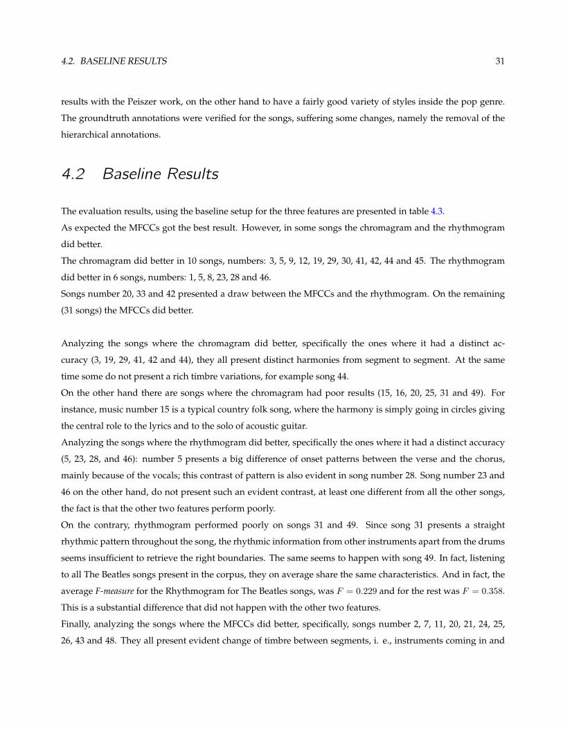
4.2. BASELINE RESULTS 31
results with the Peiszer work, on the other hand to have a fairly good variety of styles inside the pop genre.
The groundtruth annotations were verified for the songs, suffering some changes, namely the removal of the
hierarchical annotations.
4.2 Baseline Results
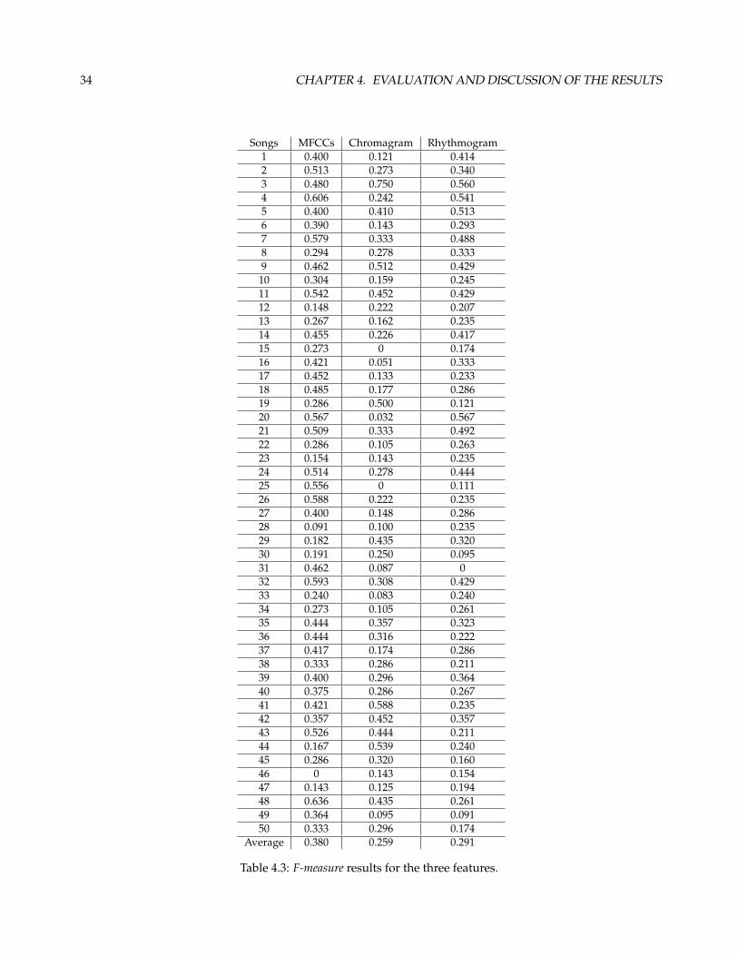
The evaluation results, using the baseline setup for the three features are presented in table 4.3.
As expected the MFCCs got the best result. However, in some songs the chromagram and the rhythmogram
did better.
The chromagram did better in 10 songs, numbers: 3, 5, 9, 12, 19, 29, 30, 41, 42, 44 and 45. The rhythmogram
did better in 6 songs, numbers: 1, 5, 8, 23, 28 and 46.
Songs number 20, 33 and 42 presented a draw between the MFCCs and the rhythmogram. On the remaining
(31 songs) the MFCCs did better.
Analyzing the songs where the chromagram did better, specifically the ones where it had a distinct ac-
curacy (3, 19, 29, 41, 42 and 44), they all present distinct harmonies from segment to segment. At the same
time some do not present a rich timbre variations, for example song 44.
On the other hand there are songs where the chromagram had poor results (15, 16, 20, 25, 31 and 49). For
instance, music number 15 is a typical country folk song, where the harmony is simply going in circles giving
the central role to the lyrics and to the solo of acoustic guitar.
Analyzing the songs where the rhythmogram did better, specifically the ones where it had a distinct accuracy
(5, 23, 28, and 46): number 5 presents a big difference of onset patterns between the verse and the chorus,
mainly because of the vocals; this contrast of pattern is also evident in song number 28. Song number 23 and
46 on the other hand, do not present such an evident contrast, at least one different from all the other songs,
the fact is that the other two features perform poorly.
On the contrary, rhythmogram performed poorly on songs 31 and 49. Since song 31 presents a straight
rhythmic pattern throughout the song, the rhythmic information from other instruments apart from the drums
seems insufficient to retrieve the right boundaries. The same seems to happen with song 49. In fact, listening
to all The Beatles songs present in the corpus, they on average share the same characteristics. And in fact, the
average F-measure for the Rhythmogram for The Beatles songs, was F = 0.229 and for the rest was F = 0.358.
This is a substantial difference that did not happen with the other two features.
Finally, analyzing the songs where the MFCCs did better, specifically, songs number 2, 7, 11, 20, 21, 24, 25,
26, 43 and 48. They all present evident change of timbre between segments, i. e., instruments coming in and
32 CHAPTER 4. EVALUATION AND DISCUSSION OF THE RESULTS
Songs1 Aha - Take on Me2 Alanis Morrisette - Head Over Feet3 Alanis Morrisette - Thank You4 Apollo 440 - Stop the Rock5 Beastie Boys - Intergalactic6 Black Eyed Peas - Cali to New York7 Britney Spears - Hit Me Baby One More Time8 Chicago - Old Days9 Chumbawamba - Thubthumping
10 Cranberries - Zombie11 dEUS - Suds and Soda12 Madonna - Like a Virgin13 Nick Drake - Northern Sky14 Nirvana - Smells Like Teen Spirit15 Norah Jones - Lonestar16 Oasis - Wonderwall17 Portishead - Wandering Star18 Prince - Kiss19 Radiohead - Creep20 R.E.M. - Drive21 Seal - Crazy22 Simply Red - Stars23 Sinead O’Connor - Nothing Compares to You24 Spice girls - Wannabe25 The Beatles - All I’ve Got to Do26 The Beatles - All My Loving27 The Beatles - Anna Go To28 The Beatles - Being for the Benefit of Mr. Kite29 The Beatles - Devil in Her Heart30 The Beatles - Don’t Bother Me31 The Beatles - Fixing a Hole32 The Beatles - Getting Better33 The Beatles - Good Morning Good Morning34 The Beatles - Hold Me Tight35 The Beatles - I Saw Her Standing There36 The Beatles - I Wanna Be Your Man37 The Beatles - It Won’t Be Long38 The Beatles - Little Child39 The Beatles - Lovely Rita40 The Beatles - Lucy in the Sky With Diamonds41 The Beatles - Misery42 The Beatles - Money43 The Beatles - Not a Second Time44 The Beatles - Please Mister Postman45 The Beatles - Roll Over Beethoven46 The Beatles - Sgt. Peppers Lonely Hearts Club Band47 The Beatles - She’s Leaving Home48 The Beatles - Till There Was You49 The Beatles - When I’m Sixty-four50 The Beatles - With a Little Help From my Friends
Table 4.2: Corpus used.
4.3. FEATURE WINDOW OF ANALYSIS 33
out. The MFCCs showed a poor performance on songs 28 and 46. Song 46, only has 4 segments, meaning 3
boundaries, what potentially reduces the likelihood of success.
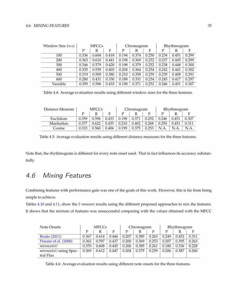
4.3 Feature Window of Analysis
The size of the windows that collects the features have a great deal of influence in the final performance of the
algorithm. Table 4.4 shows the average results using different window sizes for the three features.
The table shows that in this case the ideal window size is around the 200ms for the MFCCs, and for the other
two features the window size does not seem to be as influent.
Since the variable sized windows are between 150ms and 300ms, they obtain a result almost as good as the
fixed 200ms windows. The fact is, that computing every feature using 200ms window size is heavier than
computing the variable sized ones, then we decided to use the variable sized for further computations. Note
that the assumption of using window sizes adjusted to the structure of the song does not produce better results
as expected. Admitting that the tempo is well calculated, which was verified to happen in some songs, this may
be happening because the windows may not be fitting properly in the structure of the song, that is, must not
be starting in the first beat of the song as it was supposed.
4.4 SDM Distance Measure
As said before, the three distance measures that conveyed better results, were the Euclidean, the Manhattan
and the Cosine distance. Table 4.5 shows the average results obtained for the 50 song corpus, using the three
distance measures. It shows that the Manhattan distance got the better results for every feature. That was
expected, since the Manhattan distance performs better for high dimensionality data. Note that the rhythmo-
gram SDM is not possible to compute using the cosine distance because of the nature of the data.
4.5 Note Onsets
The attempt of using the note onsets to improve the accuracy of the method did not succeed as expected.
As shown in table 4.6, the average results for the 4 onsets tested was almost the same as without onsets, as the
introduction of the onsets did not have an influence on the final accuracy of the algorithm.
One hypothesis for this failure is the fact that there are too many note onsets in time and in that sense, some
selection would be advised. However, tests showed that using a selection window (similar to the one used for
the peak selection) and varying its size from ws to 16ws, final accuracy results showed no improvement.
34 CHAPTER 4. EVALUATION AND DISCUSSION OF THE RESULTS
Songs MFCCs Chromagram Rhythmogram1 0.400 0.121 0.4142 0.513 0.273 0.3403 0.480 0.750 0.5604 0.606 0.242 0.5415 0.400 0.410 0.5136 0.390 0.143 0.2937 0.579 0.333 0.4888 0.294 0.278 0.3339 0.462 0.512 0.429
10 0.304 0.159 0.24511 0.542 0.452 0.42912 0.148 0.222 0.20713 0.267 0.162 0.23514 0.455 0.226 0.41715 0.273 0 0.17416 0.421 0.051 0.33317 0.452 0.133 0.23318 0.485 0.177 0.28619 0.286 0.500 0.12120 0.567 0.032 0.56721 0.509 0.333 0.49222 0.286 0.105 0.26323 0.154 0.143 0.23524 0.514 0.278 0.44425 0.556 0 0.11126 0.588 0.222 0.23527 0.400 0.148 0.28628 0.091 0.100 0.23529 0.182 0.435 0.32030 0.191 0.250 0.09531 0.462 0.087 032 0.593 0.308 0.42933 0.240 0.083 0.24034 0.273 0.105 0.26135 0.444 0.357 0.32336 0.444 0.316 0.22237 0.417 0.174 0.28638 0.333 0.286 0.21139 0.400 0.296 0.36440 0.375 0.286 0.26741 0.421 0.588 0.23542 0.357 0.452 0.35743 0.526 0.444 0.21144 0.167 0.539 0.24045 0.286 0.320 0.16046 0 0.143 0.15447 0.143 0.125 0.19448 0.636 0.435 0.26149 0.364 0.095 0.09150 0.333 0.296 0.174
Average 0.380 0.259 0.291
Table 4.3: F-measure results for the three features.
4.6. MIXING FEATURES 35
Window Size (ms) MFCCs Chromagram RhythmogramP R F P R F P R F
100 0.336 0.604 0.418 0.194 0.374 0.250 0.234 0.451 0.299200 0.363 0.610 0.441 0.198 0.369 0.252 0.237 0.445 0.299300 0.346 0.579 0.420 0.198 0.379 0.252 0.238 0.448 0.300400 0.335 0.539 0.403 0.204 0.364 0.254 0.242 0.441 0.302500 0.319 0.509 0.380 0.210 0.358 0.259 0.239 0.408 0.291600 0.280 0.431 0.330 0.188 0.331 0.234 0.245 0.417 0.297
Variable 0.359 0.596 0.433 0.198 0.371 0.252 0.246 0.451 0.307
Table 4.4: Average evaluation results using different window sizes for the three features.
Distance Measure MFCCs Chromagram RhythmogramP R F P R F P R F
Euclidean 0.359 0.596 0.433 0.198 0.371 0.252 0.246 0.451 0.307Manhattan 0.377 0.622 0.455 0.210 0.402 0.268 0.250 0.451 0.311
Cosine 0.333 0.560 0.406 0.199 0.375 0.253 N.A. N.A. N.A.
Table 4.5: Average evaluation results using different distance measures for the three features.
Note that, the rhythmogram is different for every note onset used. That in fact influences its accuracy substan-
tially.
4.6 Mixing Features
Combining features with performance gain was one of the goals of this work. However, this is far from being
simple to achieve.
Tables 4.10 and 4.11, show the F-measure results using the different proposed approaches to mix the features.
It shows that the mixture of features was unsuccessful comparing with the values obtained with the MFCC
Note Onsets MFCCs Chromagram RhythmogramP R F P R F P R F
Rosao (2011) 0.367 0.614 0.446 0.207 0.389 0.263 0.249 0.452 0.311Peiszer et al. (2008) 0.362 0.597 0.437 0.200 0.369 0.253 0.207 0.395 0.263mironsets() 0.370 0.608 0.445 0.206 0.385 0.261 0.180 0.336 0.228mironsets() using Spec-tral Flux
0.369 0.612 0.447 0.204 0.379 0.259 0.206 0.387 0.260
Table 4.6: Average evaluation results using different note onsets for the three features.
36 CHAPTER 4. EVALUATION AND DISCUSSION OF THE RESULTS
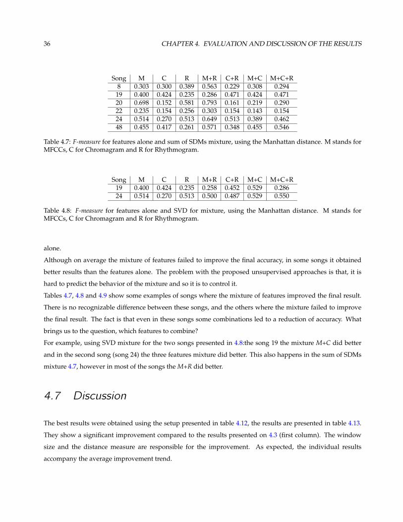
Song M C R M+R C+R M+C M+C+R8 0.303 0.300 0.389 0.563 0.229 0.308 0.29419 0.400 0.424 0.235 0.286 0.471 0.424 0.47120 0.698 0.152 0.581 0.793 0.161 0.219 0.29022 0.235 0.154 0.256 0.303 0.154 0.143 0.15424 0.514 0.270 0.513 0.649 0.513 0.389 0.46248 0.455 0.417 0.261 0.571 0.348 0.455 0.546
Table 4.7: F-measure for features alone and sum of SDMs mixture, using the Manhattan distance. M stands forMFCCs, C for Chromagram and R for Rhythmogram.
Song M C R M+R C+R M+C M+C+R19 0.400 0.424 0.235 0.258 0.452 0.529 0.28624 0.514 0.270 0.513 0.500 0.487 0.529 0.550
Table 4.8: F-measure for features alone and SVD for mixture, using the Manhattan distance. M stands forMFCCs, C for Chromagram and R for Rhythmogram.
alone.
Although on average the mixture of features failed to improve the final accuracy, in some songs it obtained
better results than the features alone. The problem with the proposed unsupervised approaches is that, it is
hard to predict the behavior of the mixture and so it is to control it.
Tables 4.7, 4.8 and 4.9 show some examples of songs where the mixture of features improved the final result.
There is no recognizable difference between these songs, and the others where the mixture failed to improve
the final result. The fact is that even in these songs some combinations led to a reduction of accuracy. What
brings us to the question, which features to combine?
For example, using SVD mixture for the two songs presented in 4.8:the song 19 the mixture M+C did better
and in the second song (song 24) the three features mixture did better. This also happens in the sum of SDMs
mixture 4.7, however in most of the songs the M+R did better.
4.7 Discussion
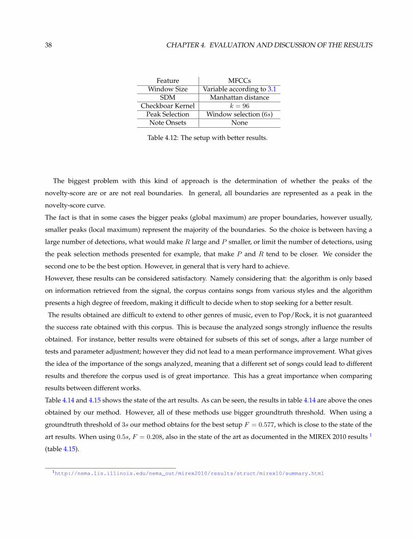
The best results were obtained using the setup presented in table 4.12, the results are presented in table 4.13.
They show a significant improvement compared to the results presented on 4.3 (first column). The window
size and the distance measure are responsible for the improvement. As expected, the individual results
accompany the average improvement trend.
4.7. DISCUSSION 37
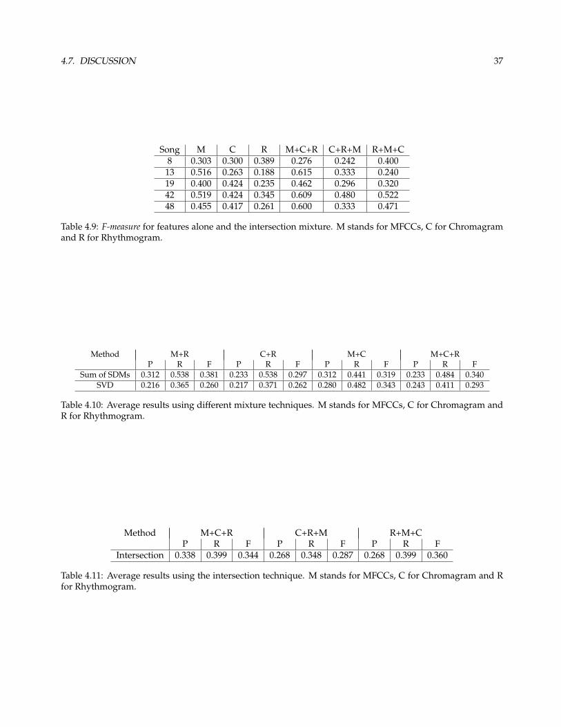
Song M C R M+C+R C+R+M R+M+C8 0.303 0.300 0.389 0.276 0.242 0.400
13 0.516 0.263 0.188 0.615 0.333 0.24019 0.400 0.424 0.235 0.462 0.296 0.32042 0.519 0.424 0.345 0.609 0.480 0.52248 0.455 0.417 0.261 0.600 0.333 0.471
Table 4.9: F-measure for features alone and the intersection mixture. M stands for MFCCs, C for Chromagramand R for Rhythmogram.
Method M+R C+R M+C M+C+RP R F P R F P R F P R F
Sum of SDMs 0.312 0.538 0.381 0.233 0.538 0.297 0.312 0.441 0.319 0.233 0.484 0.340SVD 0.216 0.365 0.260 0.217 0.371 0.262 0.280 0.482 0.343 0.243 0.411 0.293
Table 4.10: Average results using different mixture techniques. M stands for MFCCs, C for Chromagram andR for Rhythmogram.
Method M+C+R C+R+M R+M+CP R F P R F P R F
Intersection 0.338 0.399 0.344 0.268 0.348 0.287 0.268 0.399 0.360
Table 4.11: Average results using the intersection technique. M stands for MFCCs, C for Chromagram and Rfor Rhythmogram.
38 CHAPTER 4. EVALUATION AND DISCUSSION OF THE RESULTS
Feature MFCCsWindow Size Variable according to 3.1
SDM Manhattan distanceCheckboar Kernel k = 96
Peak Selection Window selection (6s)Note Onsets None
Table 4.12: The setup with better results.
The biggest problem with this kind of approach is the determination of whether the peaks of the
novelty-score are or are not real boundaries. In general, all boundaries are represented as a peak in the
novelty-score curve.
The fact is that in some cases the bigger peaks (global maximum) are proper boundaries, however usually,
smaller peaks (local maximum) represent the majority of the boundaries. So the choice is between having a
large number of detections, what would make R large and P smaller, or limit the number of detections, using
the peak selection methods presented for example, that make P and R tend to be closer. We consider the
second one to be the best option. However, in general that is very hard to achieve.
However, these results can be considered satisfactory. Namely considering that: the algorithm is only based
on information retrieved from the signal, the corpus contains songs from various styles and the algorithm
presents a high degree of freedom, making it difficult to decide when to stop seeking for a better result.
The results obtained are difficult to extend to other genres of music, even to Pop/Rock, it is not guaranteed
the success rate obtained with this corpus. This is because the analyzed songs strongly influence the results
obtained. For instance, better results were obtained for subsets of this set of songs, after a large number of
tests and parameter adjustment; however they did not lead to a mean performance improvement. What gives
the idea of the importance of the songs analyzed, meaning that a different set of songs could lead to different
results and therefore the corpus used is of great importance. This has a great importance when comparing
results between different works.
Table 4.14 and 4.15 shows the state of the art results. As can be seen, the results in table 4.14 are above the ones
obtained by our method. However, all of these methods use bigger groundtruth threshold. When using a
groundtruth threshold of 3s our method obtains for the best setup F = 0.577, which is close to the state of the
art results. When using 0.5s, F = 0.208, also in the state of the art as documented in the MIREX 2010 results 1
(table 4.15).
1http://nema.lis.illinois.edu/nema_out/mirex2010/results/struct/mirex10/summary.html
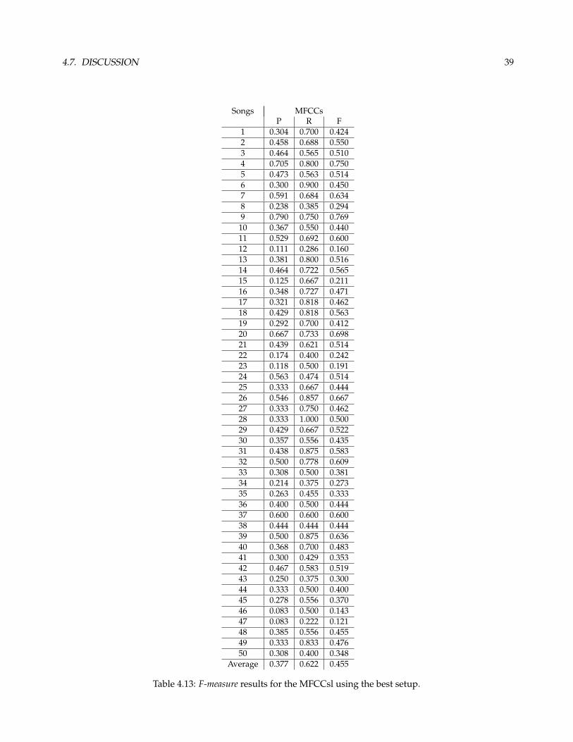
4.7. DISCUSSION 39
Songs MFCCsP R F
1 0.304 0.700 0.4242 0.458 0.688 0.5503 0.464 0.565 0.5104 0.705 0.800 0.7505 0.473 0.563 0.5146 0.300 0.900 0.4507 0.591 0.684 0.6348 0.238 0.385 0.2949 0.790 0.750 0.769
10 0.367 0.550 0.44011 0.529 0.692 0.60012 0.111 0.286 0.16013 0.381 0.800 0.51614 0.464 0.722 0.56515 0.125 0.667 0.21116 0.348 0.727 0.47117 0.321 0.818 0.46218 0.429 0.818 0.56319 0.292 0.700 0.41220 0.667 0.733 0.69821 0.439 0.621 0.51422 0.174 0.400 0.24223 0.118 0.500 0.19124 0.563 0.474 0.51425 0.333 0.667 0.44426 0.546 0.857 0.66727 0.333 0.750 0.46228 0.333 1.000 0.50029 0.429 0.667 0.52230 0.357 0.556 0.43531 0.438 0.875 0.58332 0.500 0.778 0.60933 0.308 0.500 0.38134 0.214 0.375 0.27335 0.263 0.455 0.33336 0.400 0.500 0.44437 0.600 0.600 0.60038 0.444 0.444 0.44439 0.500 0.875 0.63640 0.368 0.700 0.48341 0.300 0.429 0.35342 0.467 0.583 0.51943 0.250 0.375 0.30044 0.333 0.500 0.40045 0.278 0.556 0.37046 0.083 0.500 0.14347 0.083 0.222 0.12148 0.385 0.556 0.45549 0.333 0.833 0.47650 0.308 0.400 0.348
Average 0.377 0.622 0.455
Table 4.13: F-measure results for the MFCCsl using the best setup.
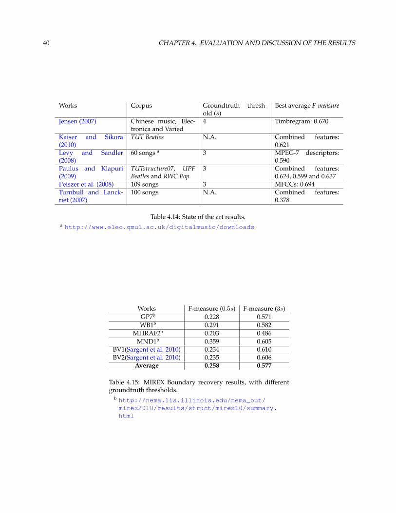
40 CHAPTER 4. EVALUATION AND DISCUSSION OF THE RESULTS
Works Corpus Groundtruth thresh-old (s)
Best average F-measure
Jensen (2007) Chinese music, Elec-tronica and Varied
4 Timbregram: 0.670
Kaiser and Sikora(2010)
TUT Beatles N.A. Combined features:0.621
Levy and Sandler(2008)
60 songs a 3 MPEG-7 descriptors:0.590
Paulus and Klapuri(2009)
TUTstructure07, UPFBeatles and RWC Pop
3 Combined features:0.624, 0.599 and 0.637
Peiszer et al. (2008) 109 songs 3 MFCCs: 0.694Turnbull and Lanck-riet (2007)
100 songs N.A. Combined features:0.378
Table 4.14: State of the art results.a http://www.elec.qmul.ac.uk/digitalmusic/downloads
Works F-measure (0.5s) F-measure (3s)GP7b 0.228 0.571WB1b 0.291 0.582
MHRAF2b 0.203 0.486MND1b 0.359 0.605
BV1(Sargent et al. 2010) 0.234 0.610BV2(Sargent et al. 2010) 0.235 0.606
Average 0.258 0.577
Table 4.15: MIREX Boundary recovery results, with differentgroundtruth thresholds.
b http://nema.lis.illinois.edu/nema_out/mirex2010/results/struct/mirex10/summary.html
4.8. SUMMARY 41
4.8 Summary
This chapter revealed the evaluation results for a variety of system setups. The baseline results showed that
the MFCCs got the better results. The window size experiments showed that the best results are obtained for
windows around 200ms. The SDM distance measure showed that the best results were obtained using the
Manhattan distance. Finally, the mixture of features and the note onsets showed no improvement to the final
performance of the method.

42 CHAPTER 4. EVALUATION AND DISCUSSION OF THE RESULTS
5Conclusion
The goal of this thesis was to perform structural segmentation on audio stream files. To that end we applied a
novelty-score approach using three features.
The features used are an attempt to represent the most important musical dimensions: the timbre, represented
by the MFCCs; the tonal space (melody and harmony), represented by the chromagram and the rhythmic space
represented by the rhythmogram.
In addition, we used mixture of features and note onsets to in an attempt to improve the final results.
The goal of this chapter is to proceed with the conclusions of the work done followed by the contributions and
finally of future work suggestions.
5.1 Conclusion
According to Bruderer et AL experiments on humans perception of structural boundaries in popular music
(Bruderer et al. 2006); ”global structure” (repetition, break), ”change in timbre”, ”change in level” and ”change
in rhythm”, represent the main perceptual cues responsible for the perceiving of boundaries in music.
In order to approximately represent such perceptual cues, we collected three features from the audio stream:
40 MFCCs, the chromagram and the rhythmogram.
Using the novelty-score approach, average results showed that the MFCCs did better, followed by the Rhyth-
mogram and finally by the chromagram. Such a ranking is consistent with the Bruderer et AL study. In the
sense that the MFCCs would represent the ”change in timbre” cue, and the rhythmogram, the ”change in
rhythm” cue. The chromagram was in fact used in order to complete the three most important musical dimen-
sions. But the fact is that, using this approach, the chromagram does not succeed. Hence, the combination of
features.
The main idea underlying the use of multiple features is that each dimension completes the others, mixing the
features was the logical action. However, mixing features proved to be a more difficult task than expected.
Three methods were tested: Intersection of peaks, sum of SDMs and the SVD. None achieved an improvement
of the average results relatively to the features alone, they all got worst mean accuracy. This leads to the con-
44 CHAPTER 5. CONCLUSION
clusion that, using the novelty-score approach the inclusion of more features and mixture is not advantageous,
as the MFCCs got the best results 4.13.
We then verify that the MFCCs are of the most importance for the task of segmenting music. Meaning that,
on average, the MFCCs encode the information that is most useful to detect the instants of change between
segments. This is on average, because as seen, in some cases the rhythmogram or the chroma encodes the most
useful information. This was the reason that lead us to experiment a way of selecting the features according to
the song.
Another effort to improve the final average results was using the note onsets to select segment boundaries.
This approach proved to be ineffective, on average did not change the final results.
Other important elements of influence in the final results are the window of analysis size and the distance
measure used to compute the SDM. To determine the window size an equation was proposed using the bpm
of the song, this got good results compared to fixed window sizes. For the distance measure, the Manhattan
distance got the best results what was expected, and is consistent with Aggarwal et al. (2001), that determined
that the Manhattan distance did better when dealing with high dimensionality data.
5.2 Contributions
The work done on Girao Antunes et al. (2011) studied: the inclusion of feature combination (MFCCs and chro-
magram) and note onsets, on a novelty-based approach to the problem of music structural segmentation.
On this thesis the work was proceeded with the inclusion of one more feature (the rhythmogram) to the mix-
ture. Also relevant was the inspection done on each music of the corpus about the results obtained with each
feature and combination, and the bpm variable window to collect the features.
5.3 Future Work
Future work should focus on: the note onsets, window of collection and feature combination. About the note
onsets, not only in terms of detection, but mostly in terms of selection. If a good selection of potential onset
candidates is done, the use of such onsets should improve the final average results. The fact is that the note
onsets used did not get worse results, results did barely change. This probably means that the note onsets were
not sufficiently selective to the novelty-score peaks, meaning that they are too close to each other and in that
sense do not influence the final result.
Moreover, one should try to improve the window adjustment to the song, to avoid features to spread to other
frames.And ensuring that windows properly fit in the structure of the song from the beginning of it.
5.3. FUTURE WORK 45
About the mixture of features some work can also be done, namely experimenting with different methods of
dimensionality reduction. And apply supervised methods to avoid that the mixture gets worst results than
the features alone.

46 CHAPTER 5. CONCLUSION
Bibliography
Aggarwal, C. C., A. Hinneburg, and D. A. Keim (2001). On the surprising behavior of distance
metrics in high dimensional space. In Lecture Notes in Computer Science, pp. 420–434.
Aucouturier, J.-J. and M.Sandler (2001). Segmentation of Musical Signals Using Hidden Markov
Models. In Proceedings of the 110th Audio Engineering Society Convention, Amsterdam, The Netherlands,
pp. 0–0.
Bello, J. P., L. Daudet, S. Abdallah, C. Duxbury, M. Davies, and M. B. Sandler (2005). A Tutorial on
Onset Detection in Music Signals. IEEE Transaction on Speech and Audio Processing 13(5), 1035–1047.
Bruderer, M. J., M. Mckinney, and A. Kohlrausch (2006). Structural Boundary Perception in Popular
Music. Time 4, 1–8.
Chu, S. and B. Logan (2000). Music Summary Using Key Phrases. April.
Cooper, M. and J. Foote (2003). Summarizing Popular Music via Structural Similarity Analysis. In
Proceedings of the 2003 IEEE Workshop on Applications of Signal Processing to Audio and Acoustics, New Platz,
NY, USA, pp. 127–130.
Dannenberg, R. B. and M. Goto (2008). Music Structure Analysis from Acoustic Signals. Handbook of
Signal Processing in Acoustics 1(April), 305–331.
Erickson, R. (1975). Sound Structure in Music.
Foote, J. (1999). Visualizing Music and Audio Using Self-Similarity. In Proceedings of the 7th ACM
international conference on Multimedia, New York, New York, USA, pp. 77–80.
Foote, J. (2000). Automatic Audio Segmentation Using A Measure of Audio Novelty. Structure.
Girao Antunes, P., D. Martins de Matos, and I. Trancoso (2011). Audio Based Segmentation Us-
ing Timbre and Chroma Features. In Proceedings of the 3rd INForum, Simposio de Informatica, Coimbra,
Portugal.
47
48 BIBLIOGRAPHY
Gomez, E. (2006). Tonal Description of Music Audio Signals. Ph. D. thesis.
Goodwin, M. M. and J. Laroche (2004). A Dynamic Programming Approach to Audio Segmentation
and Speech/Music Discrimination. In Proceedings of the IEEE International Conference on Acoustics, Speech
and Signal Processing, Montreal, Qeb., Canada, pp. 309–312.
Goto, M. (2006). A Chorus Section Detection Method for Musical Audio Signals and Its Application
to a Music Listening Station. IEEE Transactions on Audio, Speech and Language Processing 14(5), 1783–1794.
Hermansky, H. (1990). Perceptual Linear Predictive (PLP) Analysis of Speech. Journal of the Acoustical
Society of America 87(4), 1738–1752.
Jensen, K. (2004). A Causal Rhythm Grouping. pp. 83–95.
Jensen, K. (2007). Multiple Scale Music Segmentation Using Rhythm, Timbre, and Harmony.
EURASIP Journal on Advances in Signal Processing 2007, 1–12.
Kaiser, F. and T. Sikora (2010). Music Structure Discovery in Popular Music Using Non-Negative
Matrix Factorization. Journal of mathematical biology, 429–434.
Lartillot, O. (2011). MIRtoolbox 1.3.3 User’s Manual. Finnish Centre of Excelence in Interdisci-
plinary Music Research. https://www.jyu.fi/hum/laitokset/musiikki/en/research/coe/
materials/mirtoolbox.
Levy, M. and M. Sandler (2008). Structural Segmentation of Musical Audio by Constrained Cluster-
ing. IEEE Transactions on Audio, Speech, and Language Processing 16(2), 318–326.
Lu, L., M. Wang, and H.-J. Zhang (2004). Repeating Pattern Discovery and Structure Analysis from
Acoustic Music Data. In Proceedings of the 6th ACM SIGMM international workshop on Multimedia informa-
tion retrieval, New York, NY, USA, pp. 275.
Muller, M. (2007). Information Retrieval for Music and Motion. Springer Berlin Heidelberg.
Muller, M. and S. Ewert (2011). Chroma Toolbox: MATLAB Implementations for Extracting Vari-
ants of Chroma-Based Audio Features. In Proceedings of the International Conference on Music Information
Retrieval (submitted), pp. 625–636.
Paulus, J. (2010). Improving Markov Model-Based Music Piece Structure Labelling With Acous-
tic Information. In Proceedings of the 11th International Society for Music Information Retrieval Conference,
Tampere, Finland, pp. 303–308.
BIBLIOGRAPHY 49
Paulus, J. and A. Klapuri (2008). Acoustic Features for Music Piece Structure Analysis. In Proceedings
of the 11th International Conference on Digital Audio Effects, Espoo, Finland, pp. 9–12.
Paulus, J. and A. Klapuri (2009). Music Structure Analysis Using a Probabilistic Fitness Measure and
a Greedy Search Algorithm. IEEE Transactions on Audio, Speech, and Language Processing 17(6), 1159–1170.
Paulus, J., M. Muller, and A. Klapuri (2010). Audio-Based Music Structure Analysis. In Proceedings
of the 11th International Society for Music Information Retrieval Conference, Tampere, Finland, pp. 625–636.
Peeters, G. (2004). Deriving Musical Structures from Signal Analysis for Music Audio Summary
Generation : “ Sequence ” and “ State ” Approach. Springer-Verlag Berlin Heidelberg, 143–166.
Peeters, G. (2007). Sequence Representation of Music Structure Using Higher-Order Similarity Ma-
trix and Maximum-Likelihood Approach. Austrian Computer Society.
Peeters, G. and X. Rodet (2002). Toward Automatic Music Audio Summary Generation from Signal
Analysis. IRCAM - Centre Pompidou.
Peiszer, E., T. Lidy, and A. Rauber (2008). Automatic Audio Segmentation : Segment Boundary and
Structure Detection in Popular Music. Master’s thesis, Vienna University of Technology.
Rabiner, L. R. (1989). A Tutorial on Hidden Markov Models and Selected Applications in Speech
Recognition.
Rosao, C. (2011). Som em Java. Technical report, ISCTE.
Rosao, C. and R. Ribeiro (2011). Trends in onset detection. In Proceedings of the 2011 Workshop on
Open Source and Design of Communication, New York, NY, USA, pp. 75–81.
Santos, R. (2010). Music Information Retrieval: Developing Tools for Musical Content Segmentation
and Comparison. Master’s thesis, Instituto Superior Tecnico.
Sargent, G., F. Bimbot, and E. Vincent (2010). A structural segmentation of songs using generalized
likelihood ratio under regularity assumptions. In MIREX - ISMIR 2010, Utrecht, Netherlands.
Shiu, Y., H. Jeong, and C. J. Kuo (2006). Similar Segment Detection for Music Structure Analysis via
Viterbi Algorithm.
Terasawa, H., M. Slaney, and J. Berger (2005). The Thirteen Colors of Timbre. In Proceedings of the
2005 IEEE Workshop on Applications of Signal Processing to Audio and Acoustics, New Paltz, NY, USA, pp.
3–6.
50 BIBLIOGRAPHY
Turnbull, D. and G. Lanckriet (2007). A supervised approach for detecting boundaries in music using
difference features and boosting. In In Proceedings of the 5th International Conference on Music Information
Retrieval (ISMIR), pp. 42–49.
Tzanetakis, G. and P. Cook (1999). Multifeature Audio Segmentation for Browsing and Annotation.


![Error-tolerant Scribbles Based Interactive Image Segmentation · the boundary-based segmentation[9] and the scribble-based segmentation[11, 12, 1, 6, 8, 7]. The boundary-based in-teractive](https://static.fdocuments.us/doc/165x107/5f6d972e034fcd43864fa26d/error-tolerant-scribbles-based-interactive-image-segmentation-the-boundary-based.jpg)