Attributes Revisited - Rsi
21
22/1/2014 ATTRIBUTES REVISITED - RSI http://rocksolidimages.com/pdf/attrib_revisited.htm#! 1/21 ATTRIBUTES REVISITED By: M. Turhan Taner, Rock Solid Images (RSI) , Houston, Texas. 1992. (Revised May 2003) Contents Preface: Oxford Dictionary Definition of "Attribute": Definition: Introduction. Classification of Attributes. Pre-Stack Attributes. Post-Stack Attributes. Instantaneous Attributes. Wavelet Attributes. Physical Attributes. Geometrical Attributes. Reflective Attributes. Transmissive Attributes. Classification and Calibration Methods. Knowledge based Expert systems. Statistics of Attributes, Geostatistics. Linear Discrimination and PCA. Unsupervised Classification and Calibration. Supervised Training of, and Classification by, Neural Networks. Computational Procedures. Frequency Domain Computation. Discrete Time Domain Computation. Gabor-Morlet Decomposition. Simple Harmonic Motion Method. Computation of Basic Attributes. Envelope. Time Derivative of the Envelope. Second Derivative of the Envelope. Instantaneous Phase. Envelope Amplitude Modulated Phase - Intensity Varying Phase Display. Normalized Amplitude. Instantaneous Frequency. Envelope Weighted Instantaneous Frequency. Thin Bed Indicator Acceleration of Phase. Band Width. Dominant Frequency. Instantaneous Q Factor Relative Acoustic Impedance. Wavelet Attributes (Principal or Response Attributes) Geometrical Attributes. Introduction. Computation of Geometrical Attributes. Event C ontinuity. Instantaneous Dip. Instantaneous Lateral Continuity. Attributes Computed by Dip Scanning. Similarity and corresponding Dips as Lateral Continuity Attributes. Dip of Maximum Similarity. Smoothed dips of maximum similarity. Dip Variance (Local Dip versus average Dip) Loading Technology Consortia Publications Technology Oversight Board ERA Project Current Applications: Data Conditioning - AVATAR® Seismic Inversion AVO & Attributes Facies Modeling Contact RSI 2600 South Gessner, Suite 650 Houston, Texas 77063 USA +1 713 783 5593 HOME INTEGRA TED SERVICES TECHNOLOGY EXPERIENCE COMPA NY INVESTORS NEWS
-
Upload
tosinarison -
Category
Documents
-
view
271 -
download
9
Transcript of Attributes Revisited - Rsi
22/1/2014 ATTRIBUTES REVISITED - RSI
http://rocksolidimages.com/pdf/attrib_revisited.htm#! 1/21
ATTRIBUTES REVISITED
By: M. Turhan Taner, Rock Solid Images (RSI), Houston, Texas. 1992.(Revised May 2003)
Contents
Preface:
Oxford Dictionary Definition of "Attribute":
Definition:
Introduction.
Classification of Attributes.
Pre-Stack Attributes.
Post-Stack Attributes.
Instantaneous Attributes.
Wavelet Attributes.
Physical Attributes.
Geometrical Attributes.
Reflective Attributes.
Transmissive Attributes.
Classification and Calibration Methods.
Knowledge based Expert systems.
Statistics of Attributes, Geostatistics.
Linear Discrimination and PCA.
Unsupervised Classification and Calibration.
Supervised Training of, and Classification by, Neural Networks.
Computational Procedures.
Frequency Domain Computation.
Discrete Time Domain Computation.
Gabor-Morlet Decomposition.
Simple Harmonic Motion Method.
Computation of Basic Attributes.
Envelope.
Time Derivative of the Envelope.
Second Derivative of the Envelope.
Instantaneous Phase.
Envelope Amplitude Modulated Phase - Intensity Varying Phase Display.
Normalized Amplitude.
Instantaneous Frequency.
Envelope Weighted Instantaneous Frequency.
Thin Bed Indicator
Acceleration of Phase.
Band Width.
Dominant Frequency.
Instantaneous Q Factor
Relative Acoustic Impedance.
Wavelet Attributes (Principal or Response Attributes)
Geometrical Attributes.
Introduction.
Computation of Geometrical Attributes.
Event Continuity.
Instantaneous Dip.
Instantaneous Lateral Continuity.
Attributes Computed by Dip Scanning.
Similarity and corresponding Dips as Lateral Continuity Attributes.
Dip of Maximum Similarity.
Smoothed dips of maximum similarity.
Dip Variance (Local Dip versus average Dip)
Loading
TechnologyConsortia
Publications
Technology Oversight Board
ERA Project
Current Applications:
Data Conditioning - AVATAR®
Seismic Inversion
AVO & Attributes
Facies Modeling
Contact
RSI
2600 South Gessner, Suite 650
Houston, Texas 77063 USA
+1 713 783 5593
HOME INTEGRATED SERVICES TECHNOLOGY EXPERIENCE COMPANY INVESTORS NEWS
22/1/2014 ATTRIBUTES REVISITED - RSI
http://rocksolidimages.com/pdf/attrib_revisited.htm#! 2/21
Lateral Continuity.
Smoothed Similarity.
Similarity variance (instantaneous versus average)
Hybrid Attributes.
Parallel Bedding Indicator
Chaotic Reflection.
Zones of Unconformity.
Shale Indicator
FILTER DESIGN.
Band Pass Filters.
Butterworth Filter
Low Pass Butterworth Filter
High Pass Butterworth Filter
Band Pass Butterworth Filter
Minimum Phase Butterworth Filters.
Taner Filter:
Low Pass Filter
High Pass Filter
Band Pass Filter
CONVOLUTIONAL HILBERT/BUTTERWORTH FILTER.
CONVOLUTIONAL DIFFERENTIATION FILTER.
References:
Preface:
This is the third edition of the "Attributes Revisited" report. We have added a new classification of the attributes, as
we understand them at the present time. This classification may well change as our understanding of the use of
attributes improves. We give a full description of each attribute and include their projected use in interpretation. The
whole report is put in an html format to be viewed interactively by the user with any Web browser. There will also be a
printed copy available. This report contains all 2-D and 3-D post-stack and 2-D pre-stack attributes.
Oxford Dictionary Definition of "Attribute":
A quality ascribed to any person or thing.
Definition:
Seismic Attributes are all the information obtained from seismic data, either by direct measurements or by logical or
experience based reasoning.
Introduction
Based on their definition, the computation and the use of attributes go back to the origins of seismic exploration
methods. The arrival times and dips of seismic events were used in geological structure estimation. Frank Rieber in the
1940's introduced the Sonograms and directional reception. This method was extensively used in noise reduction and
time migration. The introduction of auto-correlograms and auto-convolograms (Anstey and Newman) led to better
estimates of multiple generation and more accurate use of the later developed deconvolution. NMO velocity analysis
gave better interval velocity estimates and more accurate subsurface geometries. Bright spot techniques led to gas
discoveries, as well as to some failures. This was improved by the introduction of AVO technology. Each of these
developments has helped our understanding of the subsurface and reduced the uncertainties. Unfortunately, one of the
principal failures of any of the individual techniques was our implicit dependence on it. Finally, the power of the
combined use of a number of attributes is being recognized and successful techniques are being introduced. The
attribute discussed in this paper is the outcome of the work relating to the combined use of several attributes for
lithology prediction and reservoir characterization.
Complex seismic trace attributes were introduced around 1970 as useful displays to help interpret the seismic data in a
qualitative way. Walsh of Marathon published the first article in the 1971 issue of Geophysics under the title of " Color
Sonograms". At the same time Nigel Anstey of Seiscom-Delta had published “Seiscom 1971” and introduced reflection
strength and mean frequency. He also showed color overlays of interval velocity estimates for lithological
differentiation. The new attributes were computed in the manner of radio wave reception. The reflection strength was
the result of a low pass filtered, rectified seismic trace. The color overlays showed more information than was visible on
the black and white seismic sections. Realizing the potential for extracting useful instantaneous information, Taner,
Koehler and Anstey turned their attention to wave propagation and simple harmonic motion. This led to the recognition
of the recorded signal as representing the kinetic portion of the energy flux. Based on this model, Koehler developed a
method to compute the potential component from its kinetic part. Dr. Neidell suggested the use of the Hilbert transform.
Koehler proceeded with the development of the frequency and time domain Hilbert transform programs, which made
possible practical and economical computation of all of the complex trace attributes. In the mid 70's three principal
attributes were pretty well established. Over the years a number of others were added.
The study and interpretation of seismic attributes give some qualitative information of the geometry and the physical
parameters of the subsurface. It has been noted that the amplitude content of the seismic data is the principal factor for
the determination of physical parameters, such as the acoustic impedance, reflection coefficients, velocities, absorption
etc. The phase component is the principal factor in determining the shapes of the reflectors, their geometrical
22/1/2014 ATTRIBUTES REVISITED - RSI
http://rocksolidimages.com/pdf/attrib_revisited.htm#! 3/21
configurations etc. Our objective is to bring the interpretation of attributes from a qualitative manner to a more
quantitative manner. In this paper we will first discuss the several computational methods of conventional attributes,
basically the computation of the analytic trace. In the second part we will present computation of the conventional
attributes and their derivatives. One point that must be brought out is that we define all seismically driven parameters
as the Seismic Attributes. They can be velocity, amplitude, frequency, rate of change of any of these with respect to
time or space and so on. We will classify the attributes based on their computational characteristics. They can be
computed from pre-stack or post stack data sets. Some of the attributes computed from the complex trace such as
envelope, phase etc. correspond to the various measurements of the propagating wave front. We will call these the
'Physical Attributes'. Others, computed from the reflection configuration and continuity, we will call 'Geometrical
Attributes'. The principal objectives of the attributes are to provide accurate and detailed information to the interpreter
on structural, stratigraphic and lithological parameters of the seismic prospect.
Classification of Attributes
This paper is written to provide the background information to the RSI_ATTRIB3D interactive seismic attribute
computation program developed by Seismic Research Corporation, which later became a part of Rock Solid Images.
The project was sponsored by a number of oil companies, initially by the Italian Oil Company ENI-AGIP. The initial
objective was to develop as many physical attributes as possible in order to define the lithological parameters and
reservoir characteristics from different points of view. In the development we established a general classification of
attributes based on their input data and their usage. Attributes can be computed from pre-stack or from post-stack data
before or after time migration. The procedure is the same in all of these cases. Attributes can be classified in many
different ways. Several authors have given their own classification (please see references). Here we give a classification
based on the characteristics of the attributes.
Pre-Stack Attributes
Input data are CDP or image gather traces. They will have directional (azimuth) and offset related information.
Computations generate huge amounts of data; hence they are not practical for initial studies.
Post-Stack Attributes
Stacking is an averaging process, losing offset and azimuth related information. Input data could be CDP stacked or
migrated. One should note that time migrated data will maintain their time relations, hence temporal variables, such as
frequency, will retain their physical dimensions. For depth migrated sections, frequency is replaced by wave number,
which is a function of propagation velocity and frequency. Post-stack attributes are better for observing large amounts
of data in initial investigations. For detailed studies, pre-stack attributes may be incorporated.
Computationally, we divide attributes into two general classes.
Class I attributes are computed directly from traces. This data could be pre- or post-stack, 2-D or 3-D, before or after
time migration. Trace envelope and its derivatives, instantaneous phase and its derivatives, bandwidth, Q, dips etc. are
some of the attributes computed this way.
Class II attributes are computed from the traces with improved S/N ratios after lateral scanning and semblance-
weighted summation. Details of the computation are given in the Maximum Semblance Computation section of the
Geometrical attributes. All of the Class I attributes are computed in Class II. In addition lateral continuity and dips of
maximum semblance are computed from the scanning procedure.
Based on the information content, attributes are divided into two general categories:
Instantaneous Attributes
Instantaneous attributes computed sample by sample, representing instantaneous variations of various parameters.
Instantaneous values of attributes such as trace envelope, its derivatives, frequency and phase may be determined
from complex traces. Both Class I and Class II attributes are computed.
Wavelet Attributes
Instantaneous attributes computed at the peak of the trace envelope have a direct relation to the Fourier transform of
the wavelet in the vicinity of the envelope peak. For example, Instantaneous frequency at the peak of the envelope is
equal to the mean frequency of the wavelet amplitude spectrum. Instantaneous phase corresponds to the intercept
phase of the wavelet. This attribute is also called the "response attribute". Both Class I and Class II attributes are
computed.
Another classification is based on the relation of the attributes to the geology:
Physical Attributes
Physical attributes relate to physical qualities and quantities. The magnitude of the trace envelope is proportional to the
acoustic impedance contrast, frequencies relate to the bed thickness, wave scattering and absorption. Instantaneous
and average velocities directly relate to rock properties. Consequently, these attributes are mostly used for lithological
classification and reservoir characterization.
Geometrical Attributes
Geometrical attributes describe the spatial and temporal relationship of all other attributes. Lateral continuity measured
by semblance is a good indicator of bedding similarity as well as discontinuity. Bedding dips and curvatures give
depositional information. Geometrical attributes were initially thought to help the stratigraphic interpretation. However,
further experience has shown that the geometrical attributes defining the event characteristics and their spatial
relations, quantify features that directly help in the recognition of depositional patterns, and related lithology.
Most of the attributes, instantaneous or wavelet, are assumed to study the reflected seismic wavelet characteristics.
That is, we are considering the interfaces between two beds. However, velocity and absorption are measured as
quantities occurring between two interfaces, or within a bed. Therefore, we can divide the attributes into two basic
categories based on their origin.
22/1/2014 ATTRIBUTES REVISITED - RSI
http://rocksolidimages.com/pdf/attrib_revisited.htm#! 4/21
Reflective Attributes
Attributes corresponding to the characteristics of interfaces. All instantaneous and wavelet attributes can be included
under this category. Pre-stack attributes such as AVO are also reflective attributes, since AVO studies the angle
dependent reflection response of an interface.
Transmissive Attributes
Transmissive attributes relate to the characteristics of a bed between two interfaces. Interval, RMS and average
velocities, Q, absorption and dispersion come under this category.
We will define all of the available attributes in the following sections and indicate their categories and their possible
relation to lithology, reservoir characteristics and depositional settings. In most instances individual attributes may
indicate several possible conditions, hence their logically combined use to minimize the inherent uncertainty. We call
individual attributes measuring only one quantity "Primitive" attributes. These primitive attributes may be logically
combined to form "Hybrid" attributes. This combination is knowledge based. We have several attributes of this form,
which are described later.
Gabor-Morlet type joint Time-Frequency analysis allows us to study frequency-varying attributes. Instantaneous
spectra, spectral ratio and phase differences provide measurements for bed thickness variation, absorption and
dispersion estimates.
Classification and Calibration Methods
Attribute classification helps define the combinations to be used for optimum lithology and reservoir classification. As we
have seen above, there are many different ways of computation and many different classes of attributes available.
Their utilization in quantitative interpretation is the main proof of their significance. At this time, we have defined four
different methods of classification and calibration. Here we give a short description of the methods involved. Readers
requiring further details should contact the author.
Knowledge based Expert systems
This method uses knowledge-based combinations and calibrations of groups of attributes with fuzzy logic to reflect the
interpreter’s experience. This type of classification can be used for large data sets for a quick “look-see” type of
interpretation, or when looking for a specific condition.
Statistics of Attributes, Geostatistics
These represent older and well-established methods. Cross platting with linear and various non-linear scales, measuring
various statistics have been used as viable tools. Interpolation and extrapolation between and beyond wells have been
improved by the introduction of Kriging. Incorporating the seismic and other soft information let to the development of
Co-kriging. However these methods strongly depend on the estimate of probability of each factor and provide
estimates of most likely situations of many kinds, from which the interpreter has to make the final decision.
Linear Discrimination and PCA
Principal Component Analysis (PCA) shows the principal projections where the data has the largest variance, hence the
best possible discrimination. Newly developed Independent Component Analysis (ICA) determines the projections that
are most discriminating. Linear discrimination works satisfactorily when two classes are involved and the classification
boundary is not very complicated. However, PCA and ICA are very useful analytical tools to determine the most
important attribute components to be used in the non-linear discrimination using Neural Networks.
Unsupervised Classification and Calibration
This type of approach seeks some structure in the data set. Kohonen's Self Organizing Map (SOM) method is one the
most profound methods in the Artificial Intelligence and Neural Network field. A data set may be defined by any
combination of attributes and SOM generates topologically related clusters. If the selected attributes are geometrical,
then the clusters are based on the geometrical variation. The method generates coordinates of cluster centers with
given attribute coordinates. However, it does not relate the cluster to any physical or reservoir condition. This has to be
done in the calibration stage.
Supervised Training of, and Classification by, Neural Networks
There have been a number of Neural Networks developed within the last couple of decades. Supervised trainable
networks are used in many different fields. In this case, the user provides some examples for the neural network to
learn, and then the network is tested with another data set to check the success of training. One important point to
remember is that the network, if trained properly, will recognize and correctly classify only those cases included in the
training set. Any new conditions not included in the training set will be misclassified or not recognized. Feed forward,
fully connected perceptron artificial neural networks (ANN), Learning Vector Quantization (LVQ), Probabilistic
Neural Networks (PNN), and Radial Basis Function Networks (RBF) are some of the available networks. Each of
the methods has its advantages and limitations.
Computational Procedures
We will investigate several methods of analytic trace computation. They will essentially give the same result. However,
one must keep in mind that the Hilbert transform is only valid for band limited data. For example, the Hilbert transform
of a spike is the Hilbert transform filter itself and it is infinitely long with decay of 1/t. This is contrary to the definition of
a spike. For this reason, we prefer to use band pass filter shaped, Hilbert transform time domain filters, which will be
described later.
Frequency Domain Computation
Since the real and imaginary parts of the Analytic trace are Hilbert transform pairs, then their Fourier transforms have
22/1/2014 ATTRIBUTES REVISITED - RSI
http://rocksolidimages.com/pdf/attrib_revisited.htm#! 5/21
to be causal, their amplitude spectra be the same and their phase spectra be 90 degrees out of phase. We can
therefore, form the Analytic trace by the following simple steps;
a) Transfer the seismic trace to a complex array and place it into the real part, leaving the imaginary part equal to
zero.
b) Compute the Fourier transform by FFT,
c) Zero out negative frequency components, double the positive side, but leave zero and folding frequency
components as are. This will create the causal Fourier transform of the Analytic trace.
d) The inverse Fourier transform will give an input trace that is unaltered in the real part and the imaginary part of
the output will contain the Hilbert transform of the input trace.
The frequency domain method preserves the original spectrum while generating the quadrature trace. Since almost all
computers have standard fast FFT routines, this method represents the fastest and most convenient procedure.
Discrete Time Domain Computation
The discrete Hilbert transform filter in the Time domain is an infinitely long antimetric filter with zero weights at the
center and at all even numbered samples. Its odd numbered samples have weights of 1/n. The positive side + signs
and the negative side has - signs. (Clearbout, 1976) This filter is, in theory, infinitely long, but in practice we use a
limited length filter, which causes the spectrum of the computed imaginary part to differ from the real part. The main
difficulty comes from phase discontinuities at zero and at the folding frequencies, which cannot be duplicated by finite
length filters. In order to alleviate this, we are using more convenient band-pass type filters, such as Butterworth or my
own design exponential type filters, as the Kernel functions. We design one filter to generate the real part, which is a
zero phase band pass filter. The other, a 90-degree phase rotating filter with identical band-pass characteristics, is used
to generate the imaginary part. This insures the identical amplitude spectra of both parts and excessive distortions
around zero and folding frequencies are avoided.
Gabor-Morlet Decomposition
One of the problems associated with the Hilbert transform is that it is only valid for narrow band signals. We will have an
increasing degree of uncertainty with increasing bandwidth. For example, in the extreme case, the spike is the widest
bandwidth signal and its Hilbert transform is the time domain response of the transform, which is infinitely long. This is
contrary to the locality of the spike. Luckily our data is somewhat band limited by its very nature, so we can use the
Hilbert transform to some degree. In Gabor-Morlet decomposition we divide the signal band of the original data into
smaller Gabor-Morlet bands. Gabor-Morlet filters are exponentially weighted complex cosine wavelets:
2.1)
Decomposition is done by convolving the data by a series of Gabor-Morlet wavelets generated for a sequential series of
values. Gabor wavelets were first introduced to seismic processing by Morlet et al (1982). I am enclosing a
discussion of Gabor-Morlet decomposition by Koehler at the end of this report. Since the wavelets are complex valued
and Analytic, their output will also be Analytic, complex valued. These sub-bands are summed to form the real and
imaginary parts of the wide-band Analytic trace. The sub-bands are generated equally spaced in the octave scale;
hence they do not cover the zero frequency vicinity. Usually 7-21 sub-bands are sufficient. We use this decomposition in
the spectral balancing program `SBAL'.
Simple Harmonic Motion Method
This method was our original approach, since it gave us the initial reasoning for generating the complex trace. We have
considered the geophone as a recording device, which produces electrical current proportional to the velocity of the
seismic waves arriving in the vicinity of its implantation. Therefore, the recorded data is proportional to the kinetic
portion of the energy flux at the surface. Koehler suggested that if the seismic trace were integrated, then we would
have a trace somewhat similar to the trace that we would have recorded if we could measure the position of the
geophone; thus a trace corresponding to the potential portion of the energy. Since the total energy is the same in both
components, we have to equalize the running sum of squares over some long time window. We have found that due to
this long equalization window and the effect of integration, the results are not spectrally well balanced. For this reason
we have elected not to use this method.
Computation of Basic Attributes
In this section we will cover all of the attributes computed directly from individual traces, without any additional traces in
the form of CDP gathers, common shot traces or a stacked section. We will cover attributes requiring more than one
trace at a time in the Geometrical Attribute section. We will give the mathematical formulation of each attribute and
indicate their direct and possible relation to the physical properties of the subsurface. Taner et. al. (1979) gave the
initial formulation of seismic attributes as applied to seismic data interpretation. The paper covered five attributes,
envelope amplitude, instantaneous phase, instantaneous frequency, weighted mean frequency and apparent polarity.
Their application was later discussed by Robertson and Nogami (1984) for thin bed analysis, and Robertson and Fisher
(1988) for general interpretation.
In the following pages we will cover the conventional and the new attributes. We assume that the data
going into the attribute computation have been adequately processed to contain mainly the subsurface
reflection characteristics. It is important to point out that, we highly recommend the use of 32 bit floating
point seismic data as input. 8 bit fixed point data, used regularly for visual interpretation, do not contain
sufficient dynamic range (+/-128) to produce any reliable results.
We further assume that the trace and its quadrature (Hilbert transformed component) have been computed previously,
using the original data trace for Class I and the signal to noise improved trace for Class II attributes. The rest of the
attributes are computed from this complex trace. Complex trace generation methods are covered elsewhere in this
report.
22/1/2014 ATTRIBUTES REVISITED - RSI
http://rocksolidimages.com/pdf/attrib_revisited.htm#! 6/21
Envelope
Let the Analytic trace be given by:
(3.1)
Where f(t) is the real part corresponding to the recorded seismic data and g(t), the imaginary part of the complex
trace, is the Hilbert transform of f(t). Then the envelope is the modulus of the of the complex function;
(3.2)
E(t) represents the total instantaneous energy and its magnitude is of the same order as that of the input traces. It
varies approximately between 0 and the maximum amplitude of the trace. As indicated on equation ((3.2), the envelope
is independent of the phase and it relates directly to the acoustic impedance contrasts. It may represent the individual
interface contrast or, more likely, the combined response of several interfaces, depending on the seismic bandwidth.
Trace envelope is a physical attribute and it can be used as an effective discriminator for the following characteristics:
Represents mainly the acoustic impedance contrast, hence reflectivity,
Bright spots,
Possible gas accumulation,
Sequence boundaries,
Thin-bed tuning effects
Unconformities,
Major changes of lithology,
Major changes in depositional environment,
Lateral changes indicating faulting,
Spatial correlation to porosity and other lithologic variations,
Indicates the group, rather than phase component of the seismic wave propagation,
Time Derivative of the Envelope
Time rate of change of the envelope shows the variation of the energy of the reflected events. The derivative computed
at the onset of the events shows absorption effects. A slower rise indicates larger absorption effects. We use a specially
designed time domain filter to perform the differentiation.
(3.3)
Where * denotes convolution, and diff(t) is the differentiation operator.
Events with a sharp relative rise also imply a wider bandwidth, hence less absorption effects. This attribute is also a
physical attribute and it can be used to detect possible fracturing and absorption effects.
Sharpness of the rise time relates to absorption in an inversely proportional manner,
It is affected by the slope, rather than envelope magnitude,
Lateral variation shows discontinuities,
It is used in the computation of group propagation direction. When compared with phase propagation direction, it may
indicate dispersive waves.
Second Derivative of the Envelope
The second derivative of the envelope gives a measure of sharpness of the envelope peak, which may be more useful
as a principal attribute display. In black and white displays, it shows all peaks of the envelope, this corresponds to the
all of the reflecting interfaces visible within the seismic bandwidth.
Shows all reflecting interfaces visible within seismic band-width,
Shows sharpness of events,
Indicates sharp changes of lithology,
Large changes of the depositional environment, even when the corresponding envelope amplitude may be low.
Very good presentation of the image of the subsurface within the seismic bandwidth.
Instantaneous Phase
The argument of the complex function is the instantaneous phase:
(3.4)
We display instantaneous frequency in degrees and use the color wheel to display the phase continuously. Zero degree
is displayed as yellow, +120 degrees is displayed as red (magenta) and -120 degrees (+240 degrees) displayed as blue
(cyan). All phase angles between these are color interpolated. In the default color selection we are using 64 different

22/1/2014 ATTRIBUTES REVISITED - RSI
http://rocksolidimages.com/pdf/attrib_revisited.htm#! 7/21
colors on the color wheel. This gives a rather smooth color variation in the phase display. In a number of displays we
have found that 8 different colors are sufficient. These colors represent 45-degree phase increments. The phase
information is independent of trace amplitudes and it relates to the propagation phase of the seismic wave front. Since,
most of the time, wave fronts are defined as lines of constant phase, the phase attribute is also a physical attribute and
can be effectively used as a discriminator for geometrical shape classifications:
Best indicator of lateral continuity,
Relates to the phase component of the wave-propagation.
Can be used to compute the phase velocity,
Has no amplitude information, hence all events are represented,
Shows discontinuity, but may not be the best. It is better for showing continuity.
Sequence boundaries,
Detailed visualization of bedding configurations,
Used in the computation of instantaneous frequency and acceleration,
Envelope Amplitude Modulated Phase - Intensity Varying Phase Display
Since instantaneous phase information is independent of amplitude information all of the events, including the ones with
very low amplitudes, are displayed with the same intensity. In order to show the instantaneous phase of the more
significant events, we have combined the envelope amplitude information with the phase information and it is displayed
with its own color table. The envelope amplitudes are divided into 8 different levels. Each level is represented as
successively lighter shades to indicate lower envelope amplitudes. The Color table is also divided into 8 different
regions. Each region has 8 colors similar to the original phase color wheel, except here they represent the phase in 45-
degree increments. This way the phase display shows the highest amplitude events with the most intense colors and the
weakest events will appear as the least intense, pastel colors.
Normalized Amplitude
In some instances a black and white section with balanced amplitudes similar to those of the seismic section is required
for interpretation. Conventional short window AGC application changes the reflected event characteristics; hence the
interpreters do not favor them. The display without the change of these basic characteristics is the cosine of the
instantaneous phase. This display has all the details of the instantaneous phase section and shows the desired lateral
continuity. The display has no amplitude information and its envelope is constant unity.
Instantaneous Frequency
Time rate of change of phase is the instantaneous frequency:
(3.5)
Since the phase function is multi-valued with jumps, it is better to compute the time rate of change as the
derivative of the arctangent function, which avoids the
(3.6)
Instantaneous frequency is displayed by a color table which starts with red as the lowest frequency and it gradually
changes to yellow to green and finally to blue shades for higher frequencies. The computed output is given in units of
cycles per second. Instantaneous phase represents the phase of the resultant vector of individual simple harmonic
motions. While individual vectors will rotate in clockwise motion, their resultant vector may, in some instances, form a
cardioid pattern and appear to turn in the opposite direction. We interpret this as the effect of interference of two closely
arriving wavelets. This can also be caused by the noise interference in the low amplitude zones. Because of these
reversals, the instantaneous frequency will have unusual magnitudes and fluctuations. Since instantaneous frequencies
are influenced by the bed thickness, we would like to observe them without too much interference. This we accomplish
by using several adjacent traces to form a consistent output. It has been shown that instantaneous frequency,
computed as the time derivative of instantaneous phase, relates to the centroid of the power spectrum of the seismic
wavelet.
Instantaneous frequency computation, due to its interpretational importance, has been a subject of a number of papers.
O'Doherty suggests a different way to compute the instantaneous frequency. Consider the Analytic trace F(t) and its
autocorrelation function . Let the Fourier transform of the analytic trace be represented by and the
autocorrelation function be given by . Therefore, the normalized autocorrelation function
time and frequency responses relate as:
The time derivative of the autocorrelation function corresponds to the multiplication of the power density spectrum by
iw. Therefore, the derivative computed at the zero lag represents the centroid of the power density spectrum of the
seismic event (Note that this is not the same as the instantaneous frequency computed as the time derivative of phase):
discontinuities:
(3.7)
22/1/2014 ATTRIBUTES REVISITED - RSI
http://rocksolidimages.com/pdf/attrib_revisited.htm#! 8/21
Since the derivative of the real part of the complex autocorrelation at time zero is equal to zero, the value at the first
time lag represents the phase equal to the rate of change of phase per sample. The autocorrelation function is
computed over a number of samples, which represent the averaging window. This computation, therefore, will be less
affected by superimposed reflections. Unbiased mean frequency is similar to the carrier frequency of radio signals.
Instantaneous frequencies relate the wave propagation and depositional environment, hence they are physical
attributes and they can be used as effective discriminators:
Corresponds to the average frequency (centroid) of the power spectrum of the seismic wavelet.
Seismic character correlator in lateral direction,
Indicates the edges of low impedance thin beds,
Hydrocarbon indicator by low frequency anomaly. This effect is some times accentuated by unconsolidated sands due to
the oil content of the pores.
Fracture zone indicator, they may appear as lower frequency zones.
Chaotic reflection zone indicator, due to excessive scatter,
Bed thickness indicator. Higher frequencies indicate sharp interfaces or thin shale bedding, lower frequencies indicate
sand rich bedding.
Sand/Shale ratio indicator in a clastic environment
Envelope Weighted Instantaneous Frequency
In the paragraph above, we described a method of computation of the time averaged instantaneous frequencies from
the derivative of the complex autocorrelation function. By variation of the autocorrelation computation window, we can
control the smoothing window. The shortest possible time window, one sample, should give results similar to the
derivative of the arctangent formulation. A second method of smoothing is to use the envelope, or its square (the total
power) as a weighting function for low pass filtered instantaneous frequency:
Where T is the smoothing time window.
This frequency attribute is less influenced by short wavelength effects. Longer wavelength factors, such as absorption
due to thick beds or massive sand bodies, will change the propagating wavelet characteristics that can be observed on
the weighted mean frequency attribute. It is a physical attribute, indicating longer wavelength variations.
Thin Bed Indicator
One piece of information we can extract is the locations where instantaneous frequencies jump or go in the reverse
direction. As we have discussed earlier, these jumps are indicative of closely arriving reflected wavelets. Therefore, the
time derivative of the phase function will contain the indicators for thin beds, in the form of large variations of
instantaneous frequency. Its smooth variation will relate to the bedding characteristics, which we will have to investigate
further. The thin bed indicator is, therefore, computed as the difference between the instantaneous and the time-
averaged frequencies:
(3.10)
This attribute shows the interference zones in phase. It is a physical attribute since it relates to closely spaced events. It
can be used in detailed studies:
Computed from large spikes of instantaneous frequency, indicates overlapped events
Indicates thin beds, when laterally continuous,
Indicates non-reflecting zone, when it appears laterally at random, like ‘salt and pepper’,
Shows fine detail of bedding patterns.
Acceleration of Phase
The time derivative of instantaneous frequency, by definition, gives the instantaneous acceleration. We can compute
this both from instantaneous frequency and from time averaged instantaneous frequency. It is obvious that the time
derivative of instantaneous frequency will accentuate the local frequency jumps. Consequently, it will make the thin bed
indicators more prominent. It should also indicate, to some degree, the effect of absorption by showing the frequency
dispersion of seismic signals going through unconsolidated or quickly deposited layers.
(3.11)
The acceleration computation can also be made by the O'Doherty method. The second derivative of the complex
autocorrelation function corresponds to the multiplication of the power density spectrum by the square of w. Therefore,
the second derivative computed at zero lag divided by the modulus of the autocorrelation function at the zero lag will be
equal to the acceleration;
(3.8)
(3.9)

22/1/2014 ATTRIBUTES REVISITED - RSI
http://rocksolidimages.com/pdf/attrib_revisited.htm#! 9/21
It is interesting to note that this equation is same as equation (3.15 given below. Equation (3.15 gives the square of the
RMS frequency (second moment of the power density spectrum). Here (equation (3.12) we compute the instantaneous
acceleration. The derivative of the time averaged frequency will be subtler, however, these displays need further
investigation.
Accentuates bedding differences,
Higher resolution, may have somewhat higher noise level due to differentiation,
May have some relation to elastic properties of beds.
Band Width
Barnes (1992) and O'Doherty (1992) have shown there are three attributes that relate to one another in a geometrical
or vectorial manner, similar to the statistics of observations. The frequency corresponding to the centroid of the power
spectrum of a wavelet is (we shall call it the Average Frequency):
The variance with respect to the centroid frequency is given by:
And RMS frequency (the second moment of the Power spectrum) is given by the expression:
By expanding the variance equation, we could easily show that
(3.16)
We can now examine these statistical measurements of the power spectrum in the form of useful attributes. These
computations represent the statistics of the seismic wavelet computed over some time window. Hence, they are more
closely associated with the time smoothed instantaneous attributes. We will, however, compute and display them
continuously for all of the data samples. By definition , the centroid frequency is the mean frequency where an
equal amount of energy exists on either side of this frequency.
The variance with respect to the mean frequency (standard deviation) indicates the width of power spectral density
distribution over a band of frequencies; hence we can use it as an indication of the spectral bandwidth. Barnes (1992)
suggests instantaneous bandwidth can be computed by:
(3.17)
Where denv(t)/dt is the time derivative of the envelope.
This equation measures the absolute value of the rate of change of envelope amplitude. We could also compute the
instantaneous bandwidth from the geometric equation shown above (equation (3.16) using centroid and RMS frequency
measurements. However, Barnes’ expression is simple enough to be practical. We compute and display the bandwidth
in terms of octaves.
Instantaneous bandwidth is a statistical measure of the seismic wavelet, but it relates to various physical conditions:
Represents seismic data bandwidth sample by sample. It is one of the high-resolution character correlators. Shows
overall effects of absorption and seismic character changes.
Dominant Frequency
The RMS frequency of the power density spectrum represents a biased mean towards the dominant frequency band.
Equation (3.14 gives a general idea of the computation. Following O'Doherty's reasoning we can show that the second
derivative of the normalized complex autocorrelation function will give the required results. However, we use a second
method of computation as suggested by equation (3.16. Since instantaneous frequency, computed as the time
(3.12)
(3.13)
(3.14)
(3.15)
22/1/2014 ATTRIBUTES REVISITED - RSI
http://rocksolidimages.com/pdf/attrib_revisited.htm#! 10/21
derivative of instantaneous phase, represent the mean frequency (centroid of the power spectrum), then the centroid of
the second moment of the power spectrum, or the RMS frequency, is obtained by:
(3.18)
Barnes calls this the dominant frequency. The display for this is similar to the instantaneous frequency display, in units
of cycles per second.
Instantaneous Q Factor
Barnes also suggests (in reference to definitions given by Johnston and Toksöz, 1981) that the instantaneous quality
factor q(t) can be defined by the expression:
(3.18)
Where decay(t) is the instantaneous decay rate, which is defined as the derivative of the instantaneous envelope
divided by the envelope.
Except for a factor of , this is similar to the instantaneous bandwidth. The decay rate can take both positive and
negative values. Hence, the instantaneous quality factor is the ratio of instantaneous frequency to twice the
instantaneous bandwidth. Barnes points out that this definition is consistent with the standard definitions of the quality
factor (Close, 1966 and Johnson and Toksöz, 1981). We must point out that this Q computation is the short wavelength
variation of the Q value, hence it gives relative values. It is a transmissive attribute, similar to the interval and
instantaneous velocities. It is also a physical attribute with a strong relation to porosity, permeability and fracture.
Indicates local variation of Q factor, similar to the relative acoustic impedance computation from the seismic trace.
Longer wavelength variation should be computed by spectral division and added to this attribute. May indicate liquid
content by ratioing pressure versus shear wave section Q factors. Indicates relative absorption characteristics of beds.
It is a transmissive attribute; its various wavelength components should be estimated in a similar way to the average
velocity and velocity inversion procedures.
Relative Acoustic Impedance
We assume that the seismic data has been processed to have minimum noise and multiple contamination and it contains
zero phase, wide band wavelet illumination. Based on this assumption the seismic trace represents the band limited
reflectivity series, which can be expressed as:
Which is:
Therefore, by integrating the zero phase trace, we will get the band-limited estimate of the natural log of the acoustic
impedance. Since it is band limited, the impedance will not have absolute magnitudes and the stack section is usually
the estimate of zero offset reflectivity; hence it is called relative acoustic impedance.
In practice, however, due to noise and imperfect spectral content of the seismic data, relative acoustic impedance
computed by integration will develop arbitrary long wavelength trends. Since the seismic data does not contain any
viable information at very low frequencies (due to band pass filtering in the field and during processing) these long
wavelength trends cannot be utilized. We remove these with a low cut filter.
Computation is a simple integration followed by a low pass filtering, without any exhaustive inversion. It reflects
physical property contrast, hence it is a physical attribute effectively utilized in many calibration procedures. Relative
acoustic impedance shows band limited apparent acoustic impedance contrast, It relates to porosity High contrast
indicates possible sequence boundaries, Indicates unconformity surfaces, Indicates discontinuities.
Wavelet Attributes (Principal or Response Attributes)
Wavelet (characteristic or response) attributes are, by definition, the instantaneous attributes computed at the
maximum points of the trace envelope. Intuitively, the maximum of the envelope represents a position where the
majority of the energy from different frequency bands is in phase. Therefore, attributes computed at that position would
have some direct statistical implication to the wavelet’s spectral characteristics. A number of authors (Bodine, 1984,
Barnes, 1991) have published studies of the statistics of the analytic signal and the relationship between the Fourier
transform and the instantaneous attributes. The statistics show that the attributes computed at the envelope peak relate
directly to the various moments of the power density spectrum. Therefore computation and display of these attributes
will provide an insight into the reflected wavelet characteristics. Bodine (1984) calls these attributes the `response'
attributes. I prefer the `Wavelet' attributes, because they summarize the wavelet characteristics. Since only one
attribute value is to be displayed over the length of a wavelet, we have to determine and define the wavelet length.
Definition: We assume that a seismic wavelet, or a compound wavelet, occupies the time span between two adjacent
envelope minima. In reality, wavelets will extend beyond these minima, however, for display purposes we consider the
minima as the boundary. Furthermore the part between the minima represents a significant portion of the wavelet.
Therefore, we search for the envelope minima and maxima positions. All envelope maxima positions are used to obtain
(3.19)
(3.20)
(3.21)
22/1/2014 ATTRIBUTES REVISITED - RSI
http://rocksolidimages.com/pdf/attrib_revisited.htm#! 11/21
the instantaneous attributes and these values are assigned over the time zone between the minima on either side of the
maximum position. It has been found, however, that the computation of the attributes at the sample points is not
sufficiently accurate. For example, if we consider 4 millisecond-sampled data, for a 40 Hz. wavelet each sample interval
will have a 60-degree phase difference. This is much too large to be useful. In order to be accurate, therefore, we
compute the position of the maximum of the envelope by quadratic interpolation. All of the other wavelet attributes are
also computed at the interpolated maximum position of the envelope.
The following are computed and displayed as the wavelet attributes:
Wavelet envelope
Time derivative of wavelet envelope. This attribute is computed at the onset of the wavelet at the position where the
time derivative is a maximum. It is obvious the time derivative at the envelope maximum will be zero, hence useless.
The maximum time derivative scaled by the envelope maximum will have implications of absorption.
Second derivative of wavelet envelope. This indicates the sharpness of the peak, hence some indication of bandwidth.
Wavelet phase. Lateral similarity is an excellent indication of depositional continuity.
Apparent polarity of wavelet. Polarity is assigned based on the Wavelet phase. If the phase is between -90 and +90
degrees a positive polarity is assigned, otherwise a negative polarity is assigned. Its magnitude is equal to the
interpolated envelope magnitude.
Wavelet frequency. Similar to phase, a good indicator of lateral continuity and bandwidth.
Acceleration of wavelet phase
Wavelet band width
Wavelet dominant frequency. This is direct computation of the RMS frequency of the wavelet power spectrum.
Wavelet Q factor
Wavelet attributes use the same color table as the instantaneous attributes in order keep their relationships apparent.
All of these attributes have similar discriminatory significance, but they relate to individual events, rather than to
individual samples.
Geometrical Attributes
Introduction
The phase component of seismic data contains an expanse of useful information. This information can be obtained if the
seismic trace is considered either as a complex entity, or as an analytic function consisting of the recording of the
potential and the kinetic components of the energy flux at the surface of the earth. While the measurement of the phase
and its time derivative gives direct information to the state and variation of energy in a temporal sense, the
measurement, extended to include the spatial information, yields information on the wave number and the visible
direction of propagation. It is well known that, wave propagate in two separate mode, phase and group. In dispersive
medium these two modes will have different propagation velocities. Here, we assume a non-dispersive mode and
consider the phase component only. Separate computation of phase and group propagations have been discussed by
Barnes (1994).
A further, and perhaps more important benefit, comes from the redundant information contained along the wave front
which helps to reduce the effects of noise. One of the more useful attributes, the instantaneous frequency, suffers from
the influence of noise, which breaks the spatial continuity. This appears, even in time averaged frequency displays, as
trace wide color streaks. O'Doherty (1992) has shown that by including the spatial information in the averaging process,
the instantaneous frequency and dip computations can be stabilized to the degree that the events can be tracked with
more confidence.
Let f(t,x) be the recorded seismic trace which is the real part of the complex trace, then g(t,x) is computed by Hilbert
or Gabor filtering of the f(t,x) trace, then the complex traces are defined by (now in two dimensional sense)
(4.1)
Instantaneous amplitude is given by:
(4.2)
Instantaneous phase is given by:
(4.3)
Instantaneous frequency is given by:
(4.4)
One of the main problems is the discontinuity in the phase function. It is not a continuously increasing function. This
gives rise to negative instantaneous frequencies, most likely due to the interference caused by two or more overlapped
wavelets. The main hypothesis is ``Simple seismic wavelets are such that their amplitudes rise to a maximum at a rate
proportional to their general spectral content and their phase increases continuously without any local reversal''. It has
been shown that the rise time is affected by the energy loss at higher frequencies or is due to dispersion effects. One
method of Q computation is based on the wavelet envelope rise time. According to our proposed condition of continuous
phase increase, we consider the phase reversals are due to the interference of closely spaced wavelets with opposite
22/1/2014 ATTRIBUTES REVISITED - RSI
http://rocksolidimages.com/pdf/attrib_revisited.htm#! 12/21
polarities. If we plot the hodogram (the trace vector in the complex domain) the end of the vector rotates in a counter
clockwise direction, in a somewhat circular orbit with a time varying radius. The interference appears as a cardioid
pattern that shows the resultant vector going in the opposite direction for a short time period and then proceeding in the
original direction. The average angular velocity of the vector is the mean frequency of the corresponding wavelets. This
is similar to the carrier frequencies of radio waves. In our computation we will have to compute and remove the slowly
time varying component of the angular velocity (instantaneous frequency) or the mean slope of the phase function. The
remainder will show the local deviations. These local deviations, when displayed in a sectional form, will show the thin
bed structure of the seismic data. Local deviations can also be due to the influence of the noise vector, therefore, we
have to separate the effects of the noise from those of the wavelet interference. Usually the noise effects are visible in
the zones of low signal amplitude. Interference occurs at the arrival of a second signal with larger envelope magnitudes.
This condition has led us to develop a weighted filtering scheme for smoothed instantaneous frequency determination.
This weighted frequency is a slowly varying function of time and represents, essentially, the Wavelet frequency. Since
the reflectivity function of the earth is finely structured and the wavelets used to illuminate it have, relatively, a much
longer wavelength, we are essentially observing the interference patterns, rather than a direct observation of images.
In the future we will need to develop some new methods to take advantage of the interference patterns and make
better and finer detailed estimates of the subsurface images. Thin bed indicators, instantaneous and average
frequencies were covered in the second section.
Instantaneous frequency was one of the earliest used attributes. It is the rate of change of the instantaneous phase with
respect to time, and is a temporal measurement. Similarly, spatial measurements lead to the wave numbers, which will
be useful in indicating the direction of the phase component of the propagating wave field. The Eikonal equation gives us
the relationships between the temporal and spatial variables.
Let be the wave-number (radians/meter) in the x direction and the wave number in the vertical z direction and
be the angular velocity (radians per second) and V the propagation velocity (meters/second), then a plane
harmonic wave represented in the form:
(4.5)
will satisfy the scalar wave equation. Substituting this into the wave equation we will obtain the Eikonal relationship:
(4.6)
This can also be written as:
(4.7)
The time gradient on the seismic section is , then from Eikonal equation, this is equal to:
(4.8)
which is the ratio of the horizontal wave number to temporal frequency.
In the case of finely sampled data sets ' and ` ' can be computed directly from the lateral and temporal
derivatives of the instantaneous phase function. If the data is coarsely sampled we will be subjected to spatial aliasing,
hence we cannot obtain a good measurement of dips this way. In these cases local dip scanning gives a little coarser
but more accurate results. An alternative way is to interpolate the data to finer spatial sampling intervals and then
compute the dips. However, this is not an efficient method because, during the interpolation, there is an implied step of
dip estimation in order to interpolate the aliased data properly.
Ron O'Doherty showed that the ' method of computing dips suffers in the same way as the anomalous
variations in the instantaneous frequencies. For the same reason he recommended temporal and spatial smoothing in
order to get sectional consistent dips. We are using amplitude weighted smoothing similar to the frequency smoothing in
order to minimize the effects of the low amplitude noise.
O'Doherty proposes a slightly different method of smoothing, which is done during the computation of the instantaneous
frequencies and wave numbers.
It was shown by a number of authors that the instantaneous frequency computed at the maximum of a non-complicated
wavelet (like zero or nearly zero phase wavelets) corresponds to the centroidal frequency of the power spectrum of the
wavelet:
22/1/2014 ATTRIBUTES REVISITED - RSI
http://rocksolidimages.com/pdf/attrib_revisited.htm#! 13/21
(4.9)
We know that the autocorrelation function is the inverse Fourier transform of the Power density spectrum:
(4.10)
And the zero lag of the auto-correlation function is given by:
Which is equal to the denominator of the above expression (4.9. On the other hand, the derivative of the autocorrelation
function in the frequency domain is its Fourier transform multiplied by :
(4.12)
Which is essentially the numerator of the equation (4.9. At the zero lag the exponential portion of the above expression
vanishes to give us the derivative of the complex autocorrelation function at the zero lag. We can therefore compute the
instantaneous frequency by the ratio of:
(4.13)
In order for this equation to make sense, must be uniquely defined at all frequencies and must be a
complex valued function. And, since it is a complex autocorrelation function, it should have Hermitian type symmetry -
positive lags are the complex conjugate of the negative lags. Its first derivative at the zero lag will be purely imaginary.
The imaginary part of the autocorrelation function will be zero and the first derivative of its real part will also be zero.
Therefore, the instantaneous phase of the complex autocorrelation function at time lag one will represent the amount of
phase change per sample time unit. So the instantaneous frequency, defined as radians per sample, will be given by:
(4.15)
Since instantaneous frequency is the time derivative of the instantaneous phase, equation (4.13 gives the evaluation of
this derivative at the peak of the envelope, which is described as the mean frequency:
(4.16)
It is interesting to note here that, since the autocorrelation function is complex valued, we will have 4 samples per cycle
at the folding frequency. In order to compute the instantaneous frequency correctly we have to compute the phase as
shown in equation (4.14 from zero to 180 degrees, not between -90 to +90.
O'Doherty suggests using time windows long enough to suppress the effects of the noise. A time window of the order of
an average period should be sufficient. This computation should produce instantaneous frequencies similar to the
weighted mean frequencies described above. In the computation of horizontal wave numbers however, this method
may be more convenient, since it uses less samples.
O'Doherty also suggests spatial averaging of the autocorrelation function as well as the temporal averaging. This way
the influence of noise is minimized and laterally coherent wavelet information is strengthened.
The second derivative of phase with respect to the spatial variable x shows lateral (linear) continuity. If the second
derivative is zero or near zero then the lateral change of phase is linear, hence the event is linearly continuous. Any
large second differences indicate some form of discontinuity or curvature of the arrival times of the event. For the sake
of practicality we will use linear continuity over 3 adjacent traces as the measure of lateral continuity.
However, before we consider the lateral continuity, we will look into the other lateral measurement, the wave number in
the spatial x direction. The wave number is computed in the same manner as in the temporal direction. We have
found, as mentioned above, that O'Doherty’s method, using the first derivative of the autocorrelation function in spatial
direction, has advantages and it uses less spatial samples. Therefore the wave number
(4.17)
Where is the first space lag of the autocorrelation function computed in the lateral direction. The number of
traces that are included in the autocorrelation computation controls the degree of smoothing.
According to the Eikonal equation, the ratio of temporal frequency to the spatial wave number is the time gradient of the
(4.11)
is given by:
22/1/2014 ATTRIBUTES REVISITED - RSI
http://rocksolidimages.com/pdf/attrib_revisited.htm#! 14/21
wave front arriving at the surface.
(4.18)
And,
(4.19)
Where is surface arrival angle of the wave front and is the velocity at the layer where the receivers are
implanted. Scheuer and Oldenburg (1988) have used this ratio to determine the local phase and the apparent velocity
from common shot data. This measurement is displayed as the apparent dip. By assigning the surface velocity, the
apparent dip can be converted into the exit angle of the surface arriving wave front.
(4.20)
This computation can easily be extended to 3-D data sets. Similar to the expressions given above, by introducing the
component in the y direction, we will have:
(4.21)
And;
(4.22)
Equations (4.19 and (4.22 give the time gradients measured in x and y directions. Then the maximum gradient is given
by:
(4.23)
And its azimuth will be:
(4.24)
One of the important stratigraphic measurements is the lateral continuity of the reflecting horizons (Sangree, 1988 and
Vail, 1988). We are also interested in the concordance or the consistency of the bed thickness (if they are parallel or
not). As we have discussed earlier, we will measure the linear continuity by the second order partial differences of the
phase in the lateral direction. Increasing values of second difference will indicate an increasing amount of reflection
curvature. The direction of continuity will be obtained from the dip measurements. A smoothed version of the lateral
continuity measurement can be obtained by the inclusion of more samples in the spatial and temporal directions. This is
discussed in the Dip Scan section.
Another important indicator is the location of event terminations in the form of on-lap, top-lap truncation and etc.
(Sangree and Vail). These event terminations are used to determine the stratigraphic sequence boundaries.
Determination of abrupt phase changes, as in the case of faults on a migrated section, is simple. The main difficulty is
locating gentle dip differences that might be associated with down-lap or top-lap conditions. In un-migrated data, faults
have diffraction hyperbolae, which makes them appear continuous. Migration process focuses these diffraction
hyperbolae to their origination points, thus making the discontinuities more visible. At present, we will use the computed
lateral semblance to indicate the lateral event termination and continuity. We will also consider sequence boundary
detection as one of the principal research subjects for the near future.
One way to indicate event termination is to highlight the opposite of continuity as discontinuity. That is, we will highlight
the larger values of the lateral second difference of instantaneous phase. This method will probably be less diagnostic
for the beds that merge gradually. A second method is to laterally track lines of constant phase and to indicate their
terminations. This tracking could also be carried out on narrow frequency band filtered data. We would have to observe
the consistency of truncation over several bands in order to have higher redundancy. This method will be adversely
influenced by noise and by zones of chaotic reflection. Therefore a simple method to check consistency will be
necessary.
Computation of Geometrical Attributes
There are several methods to compute geometrical attributes. Earlier in this chapter we have discussed the method
based on O'Doherty's method of smoothing in spatial and temporal directions. A second method is to compute
differences in spatial direction sample by sample. If the dips extend beyond one sample per trace this method will give
aliased results. A third method of dip scanning will overcome this difficulty. In this section we will continue to discuss the
last two methods.
Event Continuity
This is an intermediate result of a hybrid attribute computation. The objective of this attribute is to develop the lateral
continuity of peaks and troughs, and to classify the type of discontinuity. At this time all real trace positive peaks are
output as +1. and negative peaks output as -1. Everything else will be output as zero. The display therefore will show
only the peaks and troughs, all with same magnitude. The development phase will connect like peaks and establish
discontinuities. Based on the type of discontinuity, it will attempt to classify the terminations as top-lap, on-lap etc.
Instantaneous Dip
Instantaneous phase for three adjacent traces is computed. A parabolic curve is fitted to the phase values laterally, and
22/1/2014 ATTRIBUTES REVISITED - RSI
http://rocksolidimages.com/pdf/attrib_revisited.htm#! 15/21
the dip at the center trace is computed. This dip is then adjusted according to the trace interval. In 3-D data sets, phase
dips in in-line and cross-line directions are computed, from which the maximum dip direction and its azimuth are
obtained. Let dt/dx and dt/dy be the corrected dips in in-line and cross-line directions respectively, then (similar to
equations (4.23 and (4.24):
will give the maximum dip, and its direction (Instantaneous Dip Azimuth) will be:
As mentioned above, this computation is valid for dips of up to 180-degree (exclusive) phase differences. Actual dips
beyond this will produce aliased results, hence they will be misleading. In such cases dip scanning with a greater
number of traces becomes necessary. As a side note, when time migrated sections are used, it is highly recommended
that the image trace spacing should be designed to eliminate any possible aliasing problems. In most instances,
conventional surface recording intervals of 12.5 or 25 meters will be sufficient to generate images at target levels below
one second at less than half of the surface interval, without violating any sampling laws.
Instantaneous Lateral Continuity
The second difference of the instantaneous phase function is computed in in-line and cross-line directions. These
represent interface curvature in each direction. The maximum curvature is assumed to be in the same direction as the
maximum instantaneous dip. Maximum curvature is estimated similar to the maximum dip:
(4.25)
Linearly continuous events will give zero curvature. Beds with a hummocky appearance will have non-zero curvature
values. Non-reflecting zones will have highly variable curvature values in time and space. This attribute highlights the
zones of large lateral dip variation; hence it can be a good indicator of faults and fractures.
Attributes Computed by Dip Scanning
Seiscom and Digicon independently developed the Dip Scanning process in the late 1960's under the commercial names
of Seis-scan and Digi-stack, respectively. The objective of the scanning was to determine the dip of maximum lateral
continuity, and use that dip to form an average data sample to produce a trace with improved signal to noise ratio
output. To measure the similarity, semblance, which was developed in 1965 by Seiscom, was used. This information
was also used in the velocity analysis to provide the surface arrival dip as part of the stacking velocity estimate. These
estimates were later used for dip, depth and interval velocity computations. Since discontinuities are the inverse of
continuities, dip scan sections have highlighted discontinuity as well as continuity. In the late 1980's, lateral maximum
semblance values were introduced as additional geometrical attributes.
Similarity and corresponding Dips as Lateral Continuity Attributes
The objective is to compute the maximum lateral similarity (computed as semblance) and corresponding dips. This is
performed in the DIPSCN Dip scan subroutine. The subroutine accepts a user requested number of traces as input. The
center trace is assumed to be the center of scanning. All traces are assigned positive and negative distances according
to their location with respect to the center trace. Actual trace distance in in-line and cross-line are considered. This will
provide the consistency of dip measurements with respect to per unit distance. The traces are summed along the linear
alignments governed by the submitted dip ranges. The semblance values are computed for each scanned dip over a
Gaussian window in the time direction. The semblance value and the dip corresponding to the maximum semblance for
each data sample are saved as output. The semblance maxima are detected by parabolic interpretation of the
semblance values of three adjacent scanned dips. These semblance maxima are compared against the overall
maximum semblance. If the local maximum is larger, then the maximum semblance is updated, and part of the
summed trace and the corresponding dip values are transferred to the output trace and dip trace respectively. After all
of the dips have been scanned, the maximum semblance contains the semblance value for the laterally most coherent
dip within the given dip range, the dip trace contains the corresponding dips and the output trace contains the
summation of traces along the dip of maximum coherency. This last output will contain laterally most continuous events.
All three output traces are stored as attributes. The Class II attributes are computed from these lateral coherency
improved output traces.
In some instances, to further improve the lateral continuity of the traces, the scanned output is scaled by a percentage
of the semblance value. Since the semblance values lie between zero (corresponding to complete lateral dissimilarity)
and 1.0 (100 percent lateral continuity), multiplying with semblance values will enhance further the laterally continuous
events while suppressing zones of discontinuity. However, this additional process produces rather strong effects, hence
it should be used with care.
The semblance is a measure of coherent power existing between a number of traces versus the total power of all
traces, as given by;
Where is the m'th trace of the gather, and Nis the length of computation window.
The lateral similarity indication is computed as semblance that is determined by considering a user-selected number of
traces. The number of traces depends on the signal to noise ratio (poor S/N, more traces), bed curvature (more
(4.26)
22/1/2014 ATTRIBUTES REVISITED - RSI
http://rocksolidimages.com/pdf/attrib_revisited.htm#! 16/21
curvature, less traces), and higher lateral discontinuity resolution (better resolution, less traces). The semblance is
generally computed over a running 40 - to - 80-millisecond time window (shorter time windows are appropriate for wide
band data). For good S/N data, 3 adjacent traces for scanning will give higher resolution. 5 or higher numbers of traces
will tend to lose lateral discontinuities and start producing longer linear components of existing events. The dip scan
range and dip increments are input in milliseconds per trace, regardless of inline and cross line distances. However, if
the actual inline and cross-line spacing has been entered, then the dip attribute output will be correctly scaled in
milliseconds per 100 meters.
In 3-D data sets, dip scanning is done for in-line and cross-line traces separately. Each scan will output S/N improved
trace, maximum semblance and dip. These are combined to produce one dip, maximum semblance and S/N improved
trace. Computation of maximum dip and its azimuth is given earlier in this report.
In 2-D cases the output from subroutine DIPSCN is used as direct input for Class II attribute computation. In 3-D cases
the output from in-line and cross-line scans are combined by semblance weighting as:
((4.26)
Where and
Dip of Maximum Similarity
In 2-D computations output from DIPSCN is directly used. In 3-D cases, dips in the in-line and cross-line directions are
vectorially summed, as in equations (4.23 and (4.24, to determine the maximum dip and its azimuth.
Smoothed dips of maximum similarity
Computed dip values are low pass filtered to generate an unbiased running average estimate. This is an iterative
process designed to minimize the effect of local outliers and spikes. This is done several times using a weighted low
pass filter. The weights are inversely proportional of the input raw data to the computed average. This will reduce the
effect of outliers and will give a more robust estimate of the mean, close to the mode. This attribute shows the
prevailing dips in a particular depositional setting
Let D(t) be the average dip, d(t) instantaneous dips and w(i) are the weights, the average dip is computed by:
(4.27)
And the weights are computed iteratively after each pass by:
(4.28)
Where K is a constant controlling the severity of rejecting outliers. Normally K=4 could be used.
Dip Variance (Local Dip versus average Dip)
This attribute measures the difference between the instantaneous dip of maximum lateral semblance and the time
average dip. Time averaging is computed with a longer user selected time window. The averaging is an iterative
process to estimate the average closer to the mode without the effects of the outliers. This attribute shows the
anomalous dips within a uniformly layered environment. It could be used to detect small faults and permeability
barriers.
Lateral Continuity
The maximum lateral semblance as output from DIPSCN is used directly in 2-D cases. In 3-D cases the output from in-
line and cross-line scans are vectorially summed to produce the lateral continuity attribute. This attribute shows the
regions of lateral consistency, or the similarity of depositional environment. It will also show the areas where the
continuity has been disturbed.
Smoothed Similarity
Semblance values are low pass filtered to generate an unbiased running average estimate. This attribute is used in
locating zones of uniform depositional settings. It is also used in computation of hybrid attributes.
Similarity variance (instantaneous versus average)
This attribute is the difference between the instantaneous maximum lateral semblance and smoothed maximum lateral
semblance. It shows the local depositional anomalies. It may also show the zones of noise or massive non-reflecting
areas.
Hybrid Attributes
Most of the attributes discussed previously are defined as "Primitive" attributes. They basically measure a particular
physical or geometrical condition or statistic. They are primitive, but they can also be used as building blocks and, by
combining them logically, can be used to detect more complicated conditions. The logic of the combination is experience
and knowledge based. For example, the fluid factor computed by the AVO analysis is a hybrid attribute based on
experience. In this section I will give descriptions of several hybrid attributes. These are our initial attempts to combine
attributes with a knowledge-based logic. Since their introduction they have been shown to be effective discriminators.
We will continue in developing additional hybrid attributes as we incorporate an additional knowledge of Rock Physics,
are in-line and cross-line semblance scanned trace outputs,
respectively. Equation (4.26 shows that the final trace is generated by proportional summation of two traces weighted
by their percent semblance values. This output is used as the input trace for Class II computation in 3-D data sets.
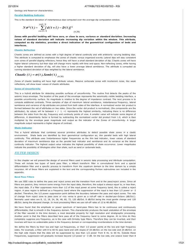
22/1/2014 ATTRIBUTES REVISITED - RSI
http://rocksolidimages.com/pdf/attrib_revisited.htm#! 17/21
Geology and Reservoir characteristics.
Parallel Bedding Indicator
This is the standard deviation of instantaneous dips computed over the average dip computation window.
(4.29)
Zones with parallel bedding will have zero, or close to zero, variance or standard deviation. Increasing
values of standard deviation will indicate increasing dip variation within the window. This attribute,
computed as dip statistics, provides a direct indication of the geometrical configuration of beds and
interfaces.
Chaotic Reflection
Chaotic zones are defined as zones with a high degree of lateral continuity and with arbitrarily varying bedding dips.
This attribute is computed to emphasize the zones of chaotic versus organized events. Lateral dips will stay consistent
over zones of parallel dipping reflectors; hence they will have a small standard deviation of dip. Chaotic zones will have
higher lateral coherency but their dips will change more rapidly with time and space. Non-reflecting zones, while having
a higher standard deviation of dip, will also have a lower average lateral semblance. The attribute is computed as
running standard deviation of dips weighted by the lateral semblance.
(4.30)
Zones of chaotic bedding will have high attribute values. Massive carbonate zones with incoherent noise, like weak
reflections, will show lower values of chaotic attributes.
Zones of Unconformity
This is a hybrid attribute for detecting possible surfaces of unconformity. The routine first detects the peaks of the
seismic trace envelope. The location of the peak of the envelope represents the seismically visible bedding interface, a
possible unconformity surface. Its magnitude is relative to the degree of impedance contrast. The next process is to
compute additional contrasts. Three samples of dips of maximum lateral semblance, instantaneous frequency, lateral
semblance and variance of dip attributes are picked from both sides of the interface. A normalized vector dot product is
formed between the set of attributes on two sides. Since the vector dot product is normalized, (the components are the
attributes), its values will lie between + /- 1. +1 represents the highest similarity, indicating there is no difference
between the sides from the dip, frequency and continuity points of view. A smaller value will indicate some degree of
difference. A dissimilarity factor is formed by subtracting the normalized vector dot product from 1.0, which is then
multiplied by the envelope peak magnitude and output as the indicator of the Zones of Unconformity. A larger
magnitude output represents a higher degree of contrast.
Shale Indicator
This a hybrid attribute that combines several primitive attributes to detect possible shale zones in a clastic
environment. Shale beds are identified by their geometrical configuration as; thin parallel beds with high lateral
continuity. This attribute uses Instantaneous higher frequencies as the thin bed indicator, lower values of standard
deviation of maximum semblance dips as the parallel bed indicator and semblance and its variance as the lateral
continuity indicator. The highest output value indicates the highest possibility of shale occurrence. Lower magnitudes
indicate the possibility of lithologies other than shale, such as sand or carbonate beds.
FILTER DESIGN
In this chapter we will present the design of several filters used in seismic data processing and Attribute computation.
These will include two types of band pass filter, a Hilbert transform filter in convolutional form and a special
differentiation filter and a specific process to transform from the cepstrum domain to the time domain by a simple
recursion. All of these filters are explained in the text and the corresponding Fortran subroutines are included in the
appendix.
Band Pass Filters
We use IEEE rules to define the pass and reject zones and the transition from and to the pass/reject zones. Since all
filters are passive, they remove some energy from the input data, therefore, the output is always equal to, or less than,
the input data. If a filter suppresses more than 1/2 of the input power at some frequency band, this is called a reject
region. A pass region is defined as a frequency band where the suppression of the input is less than 1/2 power or -3
decibel. Therefore, the 1/2 power suppression point defines the boundary between the pass and reject zones. The rate
of change from reject zone to pass zone or vice versa is given as a roll-off rate in decibel-per-Octave (dB/Oct.).
Normally used rates are 8, 12, 18, 24, 36, 48, 60, 72, 120 dB/Oct. 8 dB/Oct being the most gentle change and 120
dB/Oct. being the sharpest change. In most processing filters we use roll-off rates of 12 to 48 dB/Oct.
We have found that the amplitude or power spectrum of band-pass filters has to be continuous and continuously
differentiable; that is smooth in the frequency domain. This characteristic produces the least undulation of the envelope
of the filter wavelet in the time domain, a most desirable property for high resolution and stratigraphic processing.
Another point is that the filters described here pass all of the frequency band to some degree. At no time do they
completely suppress any frequency, as is the case with Ormsby type filters. Therefore they can be inverted, and their
inverses will have no undesirable poles in the frequency domain or corresponding reverberations in the time domain.
We define the filters by their low and high cut frequencies, or their 1/2 power points at the low and high frequency
sides. For example, a filter with 8 to 60 Hz pass band and with slopes of 18 dB/Oct. on the low side and 24 dB/Oct. on
the high side means that the data will be suppressed by less than 1/2 power from 8 Hz. to 60 Hz. Outside these
frequencies, suppression will gradually increase beyond 1/2 power or -3 dB. On the low side, one octave lower than 8
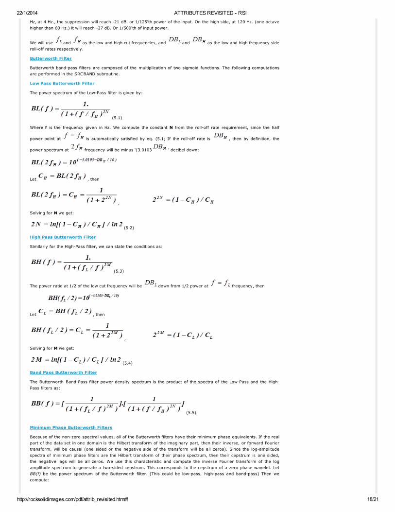
22/1/2014 ATTRIBUTES REVISITED - RSI
http://rocksolidimages.com/pdf/attrib_revisited.htm#! 18/21
Hz, at 4 Hz., the suppression will reach -21 dB. or 1/125'th power of the input. On the high side, at 120 Hz. (one octave
higher than 60 Hz.) it will reach -27 dB. Or 1/500'th of input power.
We will use and as the low and high cut frequencies, and and as the low and high frequency side
roll-off rates respectively.
Butterworth Filter
Butterworth band-pass filters are composed of the multiplication of two sigmoid functions. The following computations
are performed in the SRCBAND subroutine.
Low Pass Butterworth Filter
The power spectrum of the Low-Pass filter is given by:
(5.1)
Where f is the frequency given in Hz. We compute the constant N from the roll-off rate requirement, since the half
power point at is automatically satisfied by eq. (5.1; If the roll-off rate is , then by definition, the
power spectrum at frequency will be minus ‘(3.0103 ’ decibel down;
Let , then
,
Solving for N we get:
(5.2)
High Pass Butterworth Filter
Similarly for the High-Pass filter, we can state the conditions as:
(5.3)
The power ratio at 1/2 of the low cut frequency will be down from 1/2 power at frequency, then
Let , then
,
Solving for M we get:
(5.4)
Band Pass Butterworth Filter
The Butterworth Band-Pass filter power density spectrum is the product of the spectra of the Low-Pass and the High-
Pass filters as:
(5.5)
Minimum Phase Butterworth Filters
Because of the non-zero spectral values, all of the Butterworth filters have their minimum phase equivalents. If the real
part of the data set in one domain is the Hilbert transform of the imaginary part, then their inverse, or forward Fourier
transform, will be causal (one sided or the negative side of the transform will be all zeros). Since the log-amplitude
spectra of minimum phase filters are the Hilbert transform of their phase spectrum, then their cepstrum is one sided,
the negative lags will be all zeros. We use this characteristic and compute the inverse Fourier transform of the log
amplitude spectrum to generate a two-sided cepstrum. This corresponds to the cepstrum of a zero phase wavelet. Let
BB(f) be the power spectrum of the Butterworth filter. (This could be low-pass, high-pass and band-pass) Then we
compute:

22/1/2014 ATTRIBUTES REVISITED - RSI
http://rocksolidimages.com/pdf/attrib_revisited.htm#! 19/21
(5.6)
Since we have used only the real part with the imaginary part equal to zero, then the will be symmetrical. In
order to form the cepstrum of the minimum phase wavelet we will set the negative lags to zero:
for,
And double all values for lags larger than zero, leaving the zero lag as is:
for,
We now have the cepstrum of the minimum phase filter. Once the cepstrum of the minimum phase wavelet is obtained,
then its time domain response is computed by a simple recursion (Oppenheim and Schafer, 1975, p. 504). This is done
in the CEPTIM subroutine. Let be the n'th element of the cepstrum and the m'th element of the filter in the time
domain, then by recursion we compute later elements of the filter from earlier computed elements as:
, thus the first element will be ' and
(5.7)
Recursion will produce the rest of the filter weights. In order to have gradual reduction of filter
amplitudes down to zero at the tail end, we use Butterworth type sigmoidal tapers as used in the TAPER
subroutine.
Taner Filter:
We have found that Ricker wavelets have the most desirable shape; their envelope is a decaying exponential function.
All of the filters designed by specifying four corners of the spectrum, like Ormsby filters, will have envelopes with many
lobes. These lobes are very disagreeable for the fine definitions required by stratigraphic processing, as well as regular
processing. In order to achieve smoothness of the wavelet envelopes, I experimented with exponential functions in the
log and octave domain. Low and high pass filters are simple exponential functions, whose characteristics are controlled
by the user given band limits and roll-off rates.
Low Pass Filter
The log-amplitude spectrum of the Low-Pass filter is given by:
(5.8)
Where x is the frequency given in octaves as . If then we will have 1/2 power or
in log scale. Therefore;
We compute the constant from the roll-off rate requirement, since half power point at x=xH is automatically
satisfied by eq.(5.8.; If the roll-off rate is , then by definition the power spectrum at 1 octave higher than
frequency will be ' decibel down;
Or,
Solving for we get:
(5.9)
High Pass Filter
Similarly for the High-Pass filter, we can state the conditions as:
For we will have , hence;
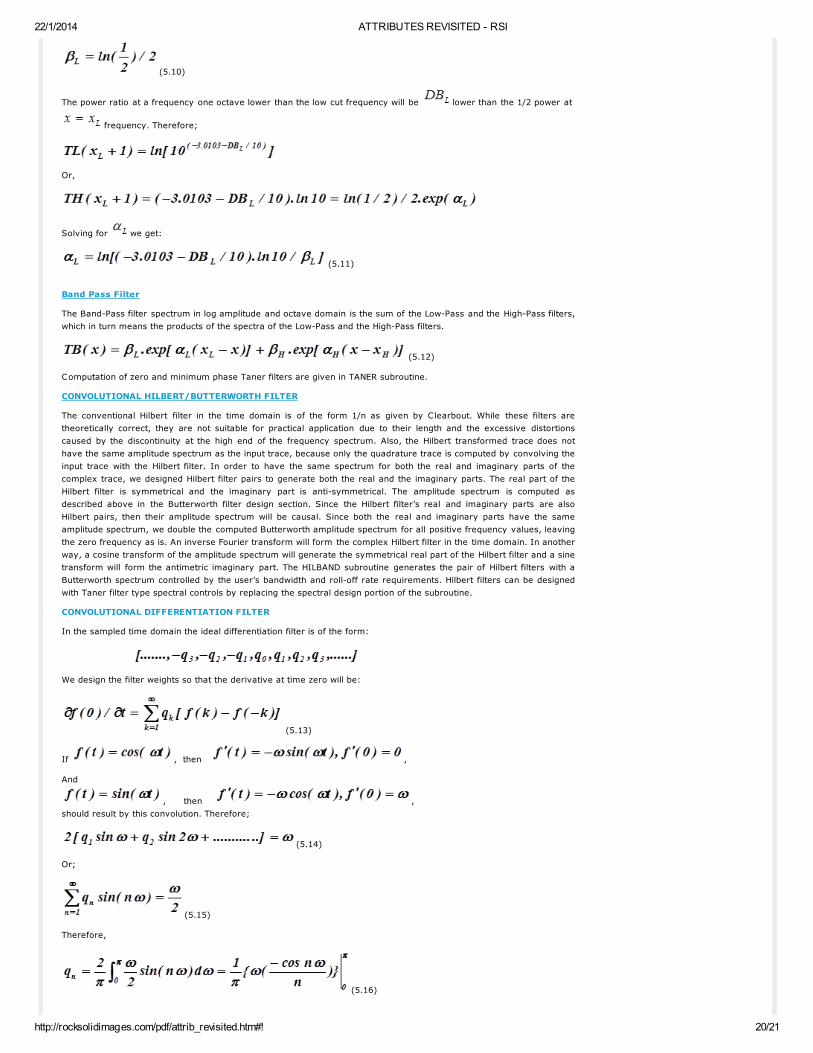
22/1/2014 ATTRIBUTES REVISITED - RSI
http://rocksolidimages.com/pdf/attrib_revisited.htm#! 20/21
(5.10)
The power ratio at a frequency one octave lower than the low cut frequency will be lower than the 1/2 power at
frequency. Therefore;
Or,
Solving for we get:
(5.11)
Band Pass Filter
The Band-Pass filter spectrum in log amplitude and octave domain is the sum of the Low-Pass and the High-Pass filters,
which in turn means the products of the spectra of the Low-Pass and the High-Pass filters.
(5.12)
Computation of zero and minimum phase Taner filters are given in TANER subroutine.
CONVOLUTIONAL HILBERT/BUTTERWORTH FILTER
The conventional Hilbert filter in the time domain is of the form 1/n as given by Clearbout. While these filters are
theoretically correct, they are not suitable for practical application due to their length and the excessive distortions
caused by the discontinuity at the high end of the frequency spectrum. Also, the Hilbert transformed trace does not
have the same amplitude spectrum as the input trace, because only the quadrature trace is computed by convolving the
input trace with the Hilbert filter. In order to have the same spectrum for both the real and imaginary parts of the
complex trace, we designed Hilbert filter pairs to generate both the real and the imaginary parts. The real part of the
Hilbert filter is symmetrical and the imaginary part is anti-symmetrical. The amplitude spectrum is computed as
described above in the Butterworth filter design section. Since the Hilbert filter’s real and imaginary parts are also
Hilbert pairs, then their amplitude spectrum will be causal. Since both the real and imaginary parts have the same
amplitude spectrum, we double the computed Butterworth amplitude spectrum for all positive frequency values, leaving
the zero frequency as is. An inverse Fourier transform will form the complex Hilbert filter in the time domain. In another
way, a cosine transform of the amplitude spectrum will generate the symmetrical real part of the Hilbert filter and a sine
transform will form the antimetric imaginary part. The HILBAND subroutine generates the pair of Hilbert filters with a
Butterworth spectrum controlled by the user’s bandwidth and roll-off rate requirements. Hilbert filters can be designed
with Taner filter type spectral controls by replacing the spectral design portion of the subroutine.
CONVOLUTIONAL DIFFERENTIATION FILTER
In the sampled time domain the ideal differentiation filter is of the form:
We design the filter weights so that the derivative at time zero will be:
(5.13)
If , then ,
And
, then ,
should result by this convolution. Therefore;
(5.14)
Or;
(5.15)
Therefore,
(5.16)

22/1/2014 ATTRIBUTES REVISITED - RSI
http://rocksolidimages.com/pdf/attrib_revisited.htm#! 21/21
Therefore the exact solution will be:
(5.17)
And,
As we can see, this operator decays by a slow 1/t rate, making a very long filter. Secondly, it will have a very sharp
edge at the folding frequency, which will create undesirable side effects on the output. In order to minimize these side
effects we have designed differentiation filters with gentler slopes on the high frequency side.
The subroutine DIFROP generates the convolutional differentiation operator.
List of References
1992-2012 RSI, all rights reserved
Hom e In teg r a ted Ser v ices Tech n olog y Ex per ien ce Com pa n y In v estor s New s © RSI 2 01 3 | +1 7 1 3 7 8 3 5 5 9 3