Attitude Determination and Control Hardware Acceptance ... · PDF fileAbstract Attitude...
62
Attitude Determination and Control Hardware Acceptance Testing for Next Generation Microsatellites by Young-Young Shen A thesis submitted in conformity with the requirements for the degree of Master of Applied Science Graduate Department of the Institute for Aerospace Studies University of Toronto c Copyright 2015 by Young-Young Shen
Transcript of Attitude Determination and Control Hardware Acceptance ... · PDF fileAbstract Attitude...

Attitude Determination and Control Hardware AcceptanceTesting for Next Generation Microsatellites
by
Young-Young Shen
A thesis submitted in conformity with the requirementsfor the degree of Master of Applied Science
Graduate Department of the Institute for Aerospace StudiesUniversity of Toronto
c© Copyright 2015 by Young-Young Shen

Abstract
Attitude Determination and Control Hardware Acceptance Testing for Next Generation
Microsatellites
Young-Young Shen
Master of Applied Science
Graduate Department of the Institute for Aerospace Studies
University of Toronto
2015
In a spacecraft development cycle, components must undergo a rigorous regime of testing,
known as acceptance testing, to ensure that they can operate in the required environment
and at the required level before being accepted for spaceflight. This thesis discusses the
acceptance testing of attitude determination and control hardware using these procedures
for four satellite missions currently under development at the time of writing in the
Space Flight Laboratory at the University of Toronto Institute for Aerospace Studies.
Focus is placed on improvements made to the acceptance testing procedures and analysis
methods for the hardware. The key contributions of the thesis are improvements to
the magnetometer functional test and calibration, rate sensor calibration, sun sensor
calibration, and reaction wheel long-form functional test. This work demonstrates that
the hardware integrated into the satellites is reliable, improving confidence in mission
success, and in some cases could improve the performance of missions on-orbit.
ii
Acknowledgements
This thesis would not have been possible without the support of some key people along
the way. I would first like to thank Dr. Robert Zee for providing me with the opportunity
to study at SFL where I got a taste of working in the space industry on real satellite
missions. I am certain that the skills I had learned here will continue to prove useful as
I continue with my studies elsewhere. I only wish I could have had more time to fully
explore the many other exciting topics I had encountered in my work.
Next, I would like to acknowledge Karan Sarda, manager of the attitude group at SFL,
with whom I’ve had the pleasure of working closely and who has directly coordinated my
work over the last two years. I appreciate the countless hours you’ve spent answering my
questions and puzzling with me over problems I had run into in my work, and also doing
everything in your power to help me make the most of my experience at SFL.
I am also grateful to the other members of the attitude group, namely Niels Roth,
Marc Fournier, Najmus Ibrahim, and Pawel Lukaszynski, for getting me started on many
of my responsibilities at SFL.
Penultimately, I would like to thank all of my fellow students and the staff at SFL
for being a part of my experience here. I have enjoyed working with you all, and I have
learned a lot from everyone I had worked with.
Last, but certainly not least, I would like to thank my parents for going to sometimes
extreme lengths to support me in my undergraduate and graduate studies at the Univer-
sity of Toronto for the last six years. I absolutely could not have made it this far without
your support.
iii

Contents
1 Introduction 1
2 Acceptance Testing 7
2.1 Magnetometers . . . . . . . . . . . . . . . . . . . . . . . . . . . . . . . . 7
2.1.1 Theory of Operation . . . . . . . . . . . . . . . . . . . . . . . . . 7
2.1.2 Testing Cycle . . . . . . . . . . . . . . . . . . . . . . . . . . . . . 8
2.1.3 Functional Test Updates . . . . . . . . . . . . . . . . . . . . . . . 8
2.1.4 Outdoor Calibration Verification . . . . . . . . . . . . . . . . . . 9
2.2 Angular Rate Sensors . . . . . . . . . . . . . . . . . . . . . . . . . . . . . 11
2.2.1 Theory of Operation . . . . . . . . . . . . . . . . . . . . . . . . . 11
2.2.2 Testing Cycle . . . . . . . . . . . . . . . . . . . . . . . . . . . . . 13
2.2.3 Reduction of Calibration Orientations . . . . . . . . . . . . . . . . 13
2.2.4 Screw Torque and Bias . . . . . . . . . . . . . . . . . . . . . . . . 19
2.3 Fine Sun Sensors . . . . . . . . . . . . . . . . . . . . . . . . . . . . . . . 21
2.3.1 Theory of Operation . . . . . . . . . . . . . . . . . . . . . . . . . 21
2.3.2 Testing Cycle . . . . . . . . . . . . . . . . . . . . . . . . . . . . . 22
2.3.3 Calibration Improvements . . . . . . . . . . . . . . . . . . . . . . 22
2.4 Reaction Wheels . . . . . . . . . . . . . . . . . . . . . . . . . . . . . . . 30
2.4.1 Theory of Operation . . . . . . . . . . . . . . . . . . . . . . . . . 30
2.4.2 Testing Cycle . . . . . . . . . . . . . . . . . . . . . . . . . . . . . 31
2.4.3 Torque Test Improvements . . . . . . . . . . . . . . . . . . . . . . 32
2.4.4 Timestamp Uniformity . . . . . . . . . . . . . . . . . . . . . . . . 45
3 Conclusion 49
Bibliography 52
iv

List of Tables
2.1 Orientation Sets for Rate Sensor Calibration . . . . . . . . . . . . . . . . 15
2.2 Reaction Wheel Torque Test Speeds and Torques . . . . . . . . . . . . . 32
2.3 Reaction Wheel Torque Test Old Metrics . . . . . . . . . . . . . . . . . . 33
v

List of Figures
1.1 Attitude Determination and Control Architecture for GNB and NEMO
Platforms . . . . . . . . . . . . . . . . . . . . . . . . . . . . . . . . . . . 2
1.2 UTIAS-SFL ADCS Hardware Testing Cycle . . . . . . . . . . . . . . . . 3
1.3 UTIAS-SFL Standard Thermal Acceptance Profile [6] . . . . . . . . . . . 5
2.1 Magnetometer Calibration Setup . . . . . . . . . . . . . . . . . . . . . . 10
2.2 UTIAS-SFL Rate Sensor . . . . . . . . . . . . . . . . . . . . . . . . . . . 12
2.3 Misalignment Angle Definitions . . . . . . . . . . . . . . . . . . . . . . . 14
2.4 Rate Sensor Calibration Orientations . . . . . . . . . . . . . . . . . . . . 15
2.5 EV9 Scale Factor vs. Orientation Set . . . . . . . . . . . . . . . . . . . . 16
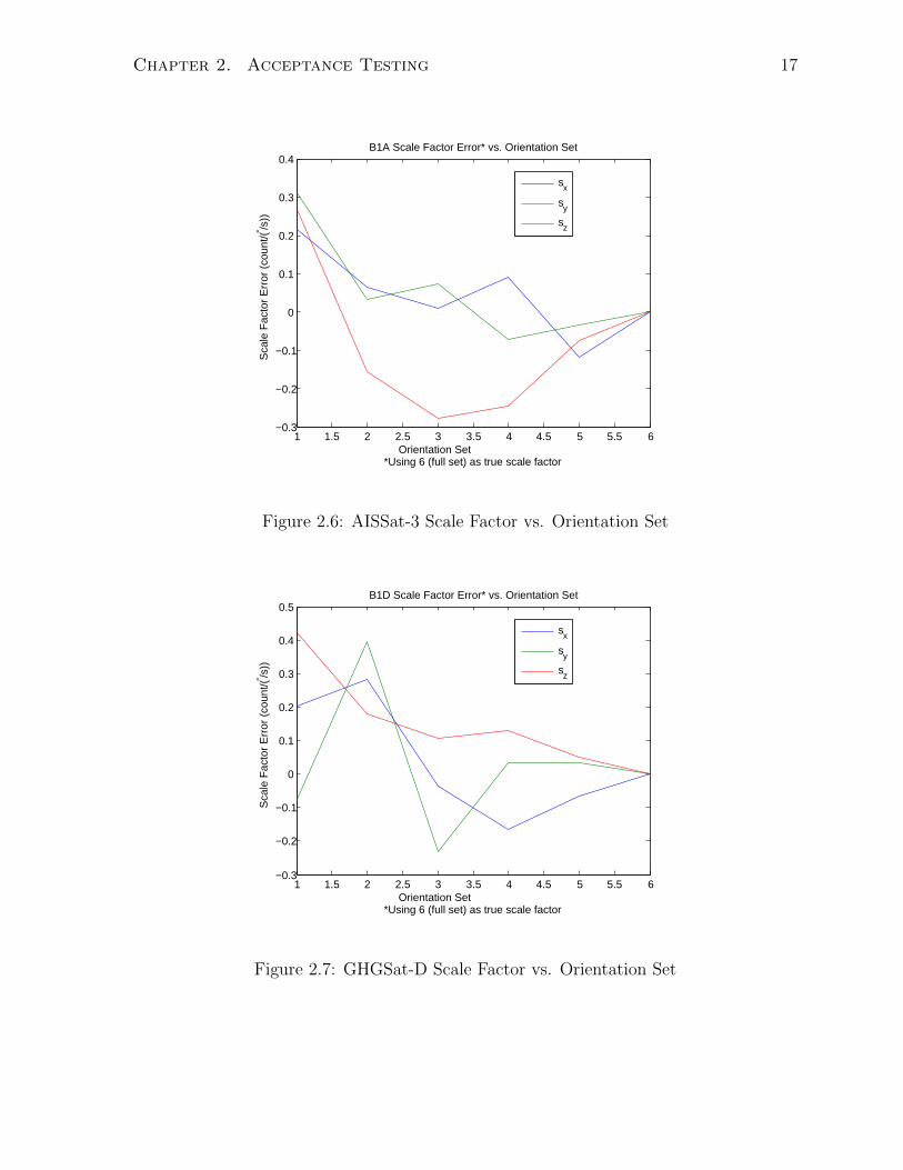
2.6 AISSat-3 Scale Factor vs. Orientation Set . . . . . . . . . . . . . . . . . 17
2.7 GHGSat-D Scale Factor vs. Orientation Set . . . . . . . . . . . . . . . . 17
2.8 EV9 Skew Angle vs. Orientation Set . . . . . . . . . . . . . . . . . . . . 18
2.9 AISSat-3 Skew Angle vs. Orientation Set . . . . . . . . . . . . . . . . . . 18
2.10 GHGSat-D Skew Angle vs. Orientation Set . . . . . . . . . . . . . . . . . 19
2.11 Screw Torque vs. Bias for Y-Axis Sensor . . . . . . . . . . . . . . . . . . 20
2.12 UTIAS-SFL Fine Sun Sensor Theory of Operation . . . . . . . . . . . . . 21
2.13 Fine Sun Sensor Calibration Setup, Side View . . . . . . . . . . . . . . . 23
2.14 Calibration Results, ρrli and ρrsr Hard-Coded . . . . . . . . . . . . . . . . 26
2.15 On Orbit vs. Simulated Sun Sensor Error . . . . . . . . . . . . . . . . . . 27
2.16 Calibration Results, ρrli and ρrsr Estimated . . . . . . . . . . . . . . . . . 29
2.17 Reaction Wheel Control Modes . . . . . . . . . . . . . . . . . . . . . . . 31
2.18 Reaction Wheel Torque Jitter FFT . . . . . . . . . . . . . . . . . . . . . 37
2.19 Torque Jitter FFT Spike on NORSAT-1 Reaction Wheel . . . . . . . . . 44
2.20 Torque Jitter FFT Spike on NEMO-HD Reaction Wheel . . . . . . . . . 46
2.21 Old WheelTerm Time Step Variation, 60 Hz Torque Test . . . . . . . . . 47
2.22 New WheelTerm Time Step Variation, 50 Hz Torque Test . . . . . . . . . 47
vi

List of Abbreviations
AIS Automatic Identification System
AISSat Automatic Identification System Satellite
BRITE Bright Target Explorer
CMOS Complementary Metal-Oxide Semiconductor
CVG Coriolis Vibratory Gyro
EV9 exactView-9
FSS Fine Sun Sensor
FFT Fast Fourier Transform
GHGSat-D Greenhouse Gas Satellite Demonstrator
GNB Generic Nanosatellite Bus
IGRF International Geomagnetic Field Reference
LEO Low Earth Orbit
LFFT Long Form Functional Test
MEMS Micro-Electromechanical System
NEMO Next-Generation Earth Monitoring and Observation
NOAA National Oceanic and Atmospheric Administration
NORSAT-1 Norwegian Satellite 1
OASYS On-board Attitude Subsystem Software
PCB Printed Circuit Board
PSD Power Spectral Density
RMS Root Mean Square
SFFT Short Form Functional Test
T-Shock Temperature Shock
UTIAS-SFLSpace Flight Laboratory at the University of Toronto Institute for
Aerospace StudiesVHF Very High Frequency
vii

List of Notation
F b Reference frame~F b Vectrix of reference frame, i.e. column matrices consisting of basis
vectors of frame F b, e.g. ~F b =[~b1
~b2~b3
]T~(·) Vector
v Column matrices, e.g. v =[v1 v2 . . . vn
]Tbi Vector ~b resolved in frame F i
A Matrix
Cbi Rotation matrix from frame F i to frame F b, i.e. vb = Cbivi
1 Identity matrix
|·| Absolute value (scalar), determinant (matrix)
〈·〉 Expected value˙(·) Time derivative
viii

Chapter 1
Introduction
Attitude determination and control refers to the determination and control of a space-
craft’s orientation in three-dimensional space. This is achieved using sensors to measure
attitude and using actuators to change it. Taken together, these sensors and actuators,
along with the software used to operate them, are referred to as a spacecraft’s attitude
determination and control system (ADCS). The ability of a spacecraft to determine and
control its attitude is often critical to accomplishing key objectives of its mission, and
is typically a defining metric of a mission’s capabilities. Many of the recent missions
developed by the Space Flight Laboratory at the University of Toronto Institute for
Aerospace Studies (UTIAS-SFL) have been enabled by improved pointing accuracy due
to advances in the lab’s technology for small satellite attitude determination and control.
For example, the satellites comprising the Bright Target Explorer (BRITE) mission, a
constellation of five astronomy nanosatellites observing brightness and temperature vari-
ations in bright stars, achieve a pointing accuracy of 12 arc-seconds within one standard
deviation [1], enabling them to direct their telescope payloads with the accuracy required
to meet their science objectives.
The generic ADCS architecture for UTIAS-SFL satellites is shown in Figure 1.1. This
architecture is used in two UTIAS-SFL small satellite platforms: the Generic Nanosatel-
lite Bus (GNB) – a 7 kg nanosatellite platform, and the Next-Generation Earth Moni-
toring and Observation (NEMO) bus – a 15 kg microsatellite platform. For the purposes
of this thesis, a nanosatellite refers to a satellite with mass between 1 kg and 10 kg, and
a “microsatellite” refers to a satellite with mass between 10 kg and 100 kg, in conformity
with the generally accepted industry definitions [2]. In the illustrated ADCS architec-
ture, reaction wheels and magnetic torquers are used as actuators. Fine sun sensors, a
magnetometer, and an angular rate sensor are used as coarse attitude sensors. Some
missions also have a star tracker for fine attitude determination. A discussion of the
1

Chapter 1. Introduction 2
ActuatorsSensors
On-board Attitude Software Subsystem
(OASYS)
Fine Sun SensorsMagnetometer Reaction Wheels
Magnetorquers
Attitude Dynamics
Star Tracker
Disturbance Torques
Commanded Attitude
Angular Rate Sensor
Figure 1.1: Attitude Determination and Control Architecture for GNB and NEMO Plat-forms
theory of operation for these devices is presented later in this thesis. Finally, the On-
board Attitude Subsystem Software (OASYS) processes sensor measurements, estimates
the spacecraft attitude state, and commands the actuators to apply a torque in order to
track a given commanded torque. An extended Kalman filter (EKF) is used to produce
state estimates and a proportional-derivative attitude control law is used as a controller.
The focus of this thesis is acceptance testing of attitude determination and control
hardware. Acceptance testing is a key part of the later stages of most spacecraft develop-
ment cycles [3]. Its purpose is to ensure that pieces of hardware designated for spaceflight
operate within the range of conditions required in the mission design, perform at the level
required by the system design, and are free of defects. This is distinguished from qual-
ification testing, which ensures that hardware of a particular design or model can be
included in the design of the spacecraft, which is usually completed in the earlier stages
of the spacecraft development cycle. The general acceptance testing cycle for ADCS
hardware is shown in Figure 1.2. Note that for some hardware, some of the steps in this
cycle are skipped or do not apply. The specifics of the testing cycle for each type of
hardware is discussed in their respective sections. The testing cycle includes four types
of tests: the functional test, the thermal shock (T-Shock) test, the thermal acceptance
campaign, and calibration.
Functional Test The purpose of a functional test is to operate hardware in a flight-

Chapter 1. Introduction 3
1. Initial Functional
2. T-Shock3. Post-T-
Shock Functional
4. Thermal Acceptance
5. Calibration6. Final
Functional
Pre-T-Shock Inspection
Post-T-Shock Inspection
Figure 1.2: UTIAS-SFL ADCS Hardware Testing Cycle
representative manner [4]. This ensures key components of the hardware are func-
tioning, but does not usually measure the performance of the hardware. UTIAS-
SFL distinguishes between two types of functional tests. A long form functional test
(LFFT) is a comprehensive test providing high confidence of a device’s function-
ality, and is usually performed before and after major environmental tests such as
a thermal acceptance test. A short form functional test (SFFT) is an abbreviated
test usually consisting only of a subset of the procedures of the LFFT to expedite
testing when only a basic assurance of a device’s functionality is needed. This may
be performed in the middle of an environmental test, or when small changes are
made to the hardware that don’t warrant an LFFT. For some ADCS hardware,
a comprehensive functional test is sufficiently simple to make it unnecessary to
distinguish between long form and short form tests.
Thermal Shock A thermal shock test subjects the hardware to sudden and extreme
changes in temperature in order to test the hardware’s capacity to survive extreme
temperature changes and to check the workmanship of solder joints on printed
circuit boards (PCBs) [5]. The rapid temperature changes cause uneven expansion
and contraction of PCB components, applying stress to them and dislodging ones
that are not properly soldered. At UTIAS-SFL, this test is normally performed by
a third-party contractor based on UTIAS-SFL specifications and is consequently
not part of the work discussed in this thesis. However, inspections of parts before
and after the T-shock are performed in-house.
Thermal Acceptance The thermal acceptance campaign is not a single test, but is
instead a series of tests that operate the test unit at various temperatures as well
as throughout changing temperatures. This ensures that the hardware is able to
tolerate the full range of temperatures required by the mission profile [6]. The
hardware is tested to two categories of temperatures – non-operational temper-
atures and operating temperatures. Non-operational temperatures refer to the

Chapter 1. Introduction 4
temperature range over which a device must be capable of being powered on while
remaining undamaged, whereas operating temperatures refer to the temperature
range over which the device must be capable of powering on and operating within
specifications. A third category of temperatures, survival temperatures, refers to
the range of temperatures over which a device must be capable of remaining free
from damage while powered off. However, devices are never subjected to these tem-
peratures during testing, and the thermal designs of UTIAS-SFL satellites prevent
devices from reaching these temperatures on orbit. Operating temperatures are
usually more stringent than non-operational temperatures, which in turn are more
stringent than survival temperatures. Non-operational and operating temperature
ranges are specified by the design of a satellite’s mission and are a function of orbit
and attitude profile. The design takes into consideration survival and operational
ranges typically provided by manufacturers of the parts out of which the devices
are constructed. General practice at UTIAS-SFL calls for these ranges to be de-
rated, i.e. applying stricter limits, leading to typical non-operational temperatures
for ADCS hardware of −30◦C to 70◦C and operational temperatures of −20◦C to
60◦C [7]. This practice allows for additional safety margin.
Figure 1.3 shows the UTIAS-SFL standard thermal testing profile. As illustrated,
the thermal testing campaign tests hardware at both their non-operational hot
and cold limits and their operating hot and cold limits, as well as throughout
temperature changes. Note that full SFFTs and LFFTs for ADCS sensors are not
usually possible during a thermal test since physical access to the sensors is required
in order to expose them to a stimulus, for example by moving them. Physical access
to the units is restricted once they are placed in the thermal chamber. Note also
that the temperature extremes shown in the figure are labeled as “survival” hot
and cold temperatures, a typical albeit misleading internal shorthand for a device’s
non-operational temperatures.
Calibration A calibration is a characterization of the performance of a piece of hard-
ware. This is usually performed only for ADCS sensors. In general, a calibration
involves comparing measurements made by a sensor against a set of reference mea-
surements that are known to be accurate in order to calculate the value of correction
factors. These correction factors are applied on orbit when measurements from the
sensor are used. Details of the calibration techniques for some sensors are provided
in later sections.
Note that while satellite components must also in general be tested to survive in the hard

Chapter 1. Introduction 5UTIAS/SFL Thermal Vacuum and Standard Thermal Test Procedure, Issue 1.2, 2009/06/04
UTIAS/SFL, Tel (416) 667-7864, E-mail: [email protected], UTIAS/SFL Confidential Page 4 of 6
Standard Temperature
25 deg C
T_hot, survival
T_cold, survival
T_hot
T_cold
Long-Form Functional
Test (LFFT)
Temperature
Soak, for t_soak
Warm Start + LFFT
Cold Start +
LFFT
Temperature
Soak, for t_soak
Final LFFT
All Slews at
2 deg C / min
Temperature Soak, for t_soak
Temperature
Soak, for t_soak
Temperature Soak, for t_soak
Temperature
Soak, for t_soak
Phase IV – Temperature Cycling – Check Telemetry and Communications at Regular Intervals (short-form test every t_sfft seconds)
Phase I – Initial Check Phase II – Warm Start Phase III – Cold Start Phase V –
Final Check
Temperature Profile for Unit Thermal Vacuum or Standard Thermal Tests
Figure 1.3: UTIAS-SFL Standard Thermal Acceptance Profile [6]
vacuum of space, vacuum testing is only performed at the system, or satellite, level if the
component has already been qualified in thermal vacuum.
The contribution of this thesis was to perform acceptance testing of ADCS hard-
ware for the exactView-9 (EV9), Automatic Identification System Satellite 3 (AISSat-
3), Greenhouse Gas Satellite Demonstrator (GHGSat-D), and Norwegian Satellite 1
(NORSAT-1) missions. EV9 and AISSat-3 are two ship-tracking nanosatellites based
on the Generic Nanosatellite Bus platform [8][9]. The main role of the attitude deter-
mination and control subsystem for these satellites is to point a very high frequency
(VHF) antenna to nadir, or Earthward, in order to receive positioning broadcasts from
ships. GHGSat-D is a mission that will demonstrate space-based monitoring of indus-
trial greenhouse gas emissions using a microsatellite based on the NEMO platform [10].
Attitude determination and control is used to allow the satellite to track fixed ground
targets with high accuracy as it passes over them to enable measuring of greenhouse gas
emissions from a single industrial site. Finally, NORSAT-1 is a science microsatellite also
based on the NEMO platform that will carry a radiometer for studying variations in solar
irradiance and a pair of Langmuir probes to study the plasma environment in low Earth
orbit (LEO) [11]. The satellite will also carry an AIS payload. Attitude determination
and control will be used to point the radiometer payload continuously at the Sun while
keeping the Langmuir probes pointed in the local velocity direction. GHGSat-D has the
most stringent pointing accuracy requirements of the four missions.
Testing for each mission was completed according to project timelines handed down

Chapter 1. Introduction 6
from the system-level design of the satellites. The goal of the testing was to ensure
not only that all hardware passed each test in its testing cycle, but also to ensure that
existing test procedures and acceptance criteria appropriately reflected system require-
ments. Where necessary, previously established test procedures and acceptance criteria
were adjusted, and new test procedures and criteria were developed. The testing of
ADCS hardware contributed by this thesis will help ensure to a high degree of confidence
that the satellites using the hardware will be capable of achieving the pointing objectives
required by their missions.

Chapter 2
Acceptance Testing
The sections in this chapter treat the acceptance testing of each type of attitude determi-
nation and control hardware involved in this thesis. Each section begins with a discussion
of the theory of operation of the device, followed by a description of its specific accep-
tance testing cycle, and then identifies the contributions of this thesis to the acceptance
testing of that device.
2.1 Magnetometers
2.1.1 Theory of Operation
Magnetometers are used to measure the magnitude and direction of the local magnetic
field. Combined with a model of the geomagnetic field, these can be used to determine
a satellite’s attitude about two axes at any point in its orbit. A single magnetometer
measurement leaves uncertainty in attitude about the local magnetic field vector, and
is usually combined with a measurement of another vector to obtain a full attitude
solution. UTIAS-SFL’s in-house magnetometers use three magneto-inductive sensors
oriented orthogonally to each other to measure the components of the magnetic field
vector. These sensors have the property that their inductance is proportional to the
magnetic field applied along their axes. An interface circuit measures this inductance
and converts it into a magnetic field strength value. In pointing budgets for UTIAS-SFL
missions, the magnetometer is expected to achieve an accuracy on the order of 3◦ [12] to
5◦ [13].
Due to their ability to make measurements at any point in a satellite’s orbit as well as
their relatively low cost, magnetometers have become ubiquitous in UTIAS-SFL missions.
7
Chapter 2. Acceptance Testing 8
2.1.2 Testing Cycle
The testing cycle for magnetometers at UTIAS-SFL follows the general cycle identified
in Figure 1.2. This thesis contributes updates to the functional and calibration tests for
UTIAS-SFL’s magnetometers in addition to performing the acceptance testing for the
EV9, AISSat-3, GHGSat-D, and NORSAT-1 magnetometers.
2.1.3 Functional Test Updates
A functional test of the magnetometer involves a polarity check, noise measurement, and
a rough test of sensor bias [14]. The purpose of the polarity check is to ensure that
measurements qualitatively respond in the right way to a change in the applied magnetic
field. Previously, the polarity check called for placing a permanent magnet close to the
sensor [15]. The change in the observed magnetic field along each axis should be positive
when aligned with the magnet south-to-north and negative when aligned with it north-
to-south. However, this test carried a risk of permanently magnetizing components on
the magnetometer or damaging the magneto-inductive sensors due to the strength of the
permanent magnet. It was observed that the ambient magnetic field within the lab was
sufficiently strong and consistent to be used in place of the permanent magnet in the
polarity check. Specifically, the ambient field seemed always to be the strongest along
the local vertical and in the downward direction, and was strong enough to be greater
than both the typical noise and bias levels of the magnetometer. A new procedure was
developed for the polarity check in which the magnetometer would be polled continuously
while being held in a series of orientations to align each axis with the vertical. Since the
field in the lab is known to be dominated by the vertical component in the downward
direction, the test would check that the field measured by each axis would measure a
positive field when pointed downward, and change to a negative field when flipped to
point upward.
Another update to the functional test procedure was the addition of the rough bias
check. During calibration of the magnetometer for the GHGSat-D mission, it was noticed
that measurements on one axis exhibited an abnormally large bias of approximately
23µT , where typical biases have been observed to be in the low thousands of nano-
Tesla. Additional testing confirmed that the bias was inherent to the sensor and not a
result of experimental error. Despite this bias, the unit was accepted for the mission
as a spare since it was determined that, even with the bias, the maximum expected on-
orbit field measurement on any axis (36µT unbiased) would fall well within the sensor’s
measurement range of ±131µT , and that the unit was functioning properly otherwise.

Chapter 2. Acceptance Testing 9
However, since no attempt at measuring the bias was made prior to calibration, it was
unclear at what point the bias had changed, or if it had always been high. It was therefore
decided to add a bias check to the functional test. In a similar vein to the polarity check,
the bias check consisted of aligning each axis of the sensor with the vertical while polling
for one minute, then inverting the alignment and polling for another minute. The bias for
each axis is estimated by summing the average fields measured in positive and negative
alignment. This bias check revealed through the acceptance testing campaign of the
NORSAT-1 magnetometers that a large bias similar to that seen on the GHGSat-D
sensor only appeared once the magnetometer was integrated into an interface plate that
mounts the sensor to the calibration facility. The cause of this bias was traced to a
magnetic threaded helical insert used in this plate. The helical inserts have since been
replaced with nonmagnetic titanium substitutes. Another benefit of adding this check
to the magnetometer functional test is that it could help detect faulty units with biases
outside of manufacturer specifications early in the acceptance testing cycle. This helps
reduce schedule cost in the event of a faulty sensor since replacement sensors can be
ordered before most of the testing is done rather than after calibration is completed near
the end of the cycle.
2.1.4 Outdoor Calibration Verification
The magnetometer calibration compares measurements of a series of applied magnetic
fields made by an uncalibrated “flight” magnetometer with those made by a calibrated
“lab” magnetometer in order to calculate a number of calibration parameters. The
magnetometers are mounted side-by-side on an aluminum L-bracket, which is secured
to a platform in the center of three pairs of orthogonal Helmholtz coils that generate
the applied magnetic fields. Figure 2.1 shows the magnetometer calibration setup. The
parameters determined from the calibration are programmed into OASYS, the attitude
determination and control software, to be used for estimating the true magnetic field
based on measured values and include factors that correct for sensor bias, nonlinearity of
the magnetometer’s measurements, and non-orthogonality of its axes, as well as scaling
factors for converting between the magnetometer’s native units, or “counts”, to nano-
Tesla [14].
Previous iterations of the calibration procedure were considered complete once these
parameters had been determined. However, in order to provide an additional measure
of confidence for calibrations performed with a newly commissioned in-house calibration
facility, it was decided to implement a test to verify the parameters extracted from cal-

Chapter 2. Acceptance Testing 10
Lab Magnetometer Flight Magnetometer
Helmholtz Coil (1 of 6)
Aluminum L Bracket
Figure 2.1: Magnetometer Calibration Setup
ibration. In this test, both the lab and flight magnetometers are brought outside of the
magnetically noisy lab environment and into a field far away from buildings and machin-
ery. The two magnetometers are held in a fixed orientation using the same L-bracket
from the calibration setup, and measurements of the ambient geomagnetic field are col-
lected for five minutes from both magnetometers. The calibration parameters are applied
to the flight magnetometer measurements and the corrected average field is compared
against that measured by the lab magnetometer. The error between the corrected flight
magnetometer measurement and the lab magnetometer measurement has been found to
be typically below 0.5◦ in direction and 0.6% in magnitude within 3 standard deviations.
This provides an estimate of the calibration error contributed by variations in the indoor
magnetic field that was applied to the flight and lab magnetometers during calibration.
Other contributions to the calibration error include mounting misalignment between the
lab and flight magnetometers due to manufacturing tolerances in the placement of holes
for screws and the calibration error of the lab magnetometer. The mounting misalignment
contributes up to 1.42◦ within 3 standard deviations. The lab magnetometer calibration
is accurate to 0.5% on any axis [16], which corresponds to 0.29◦ peak error. No confi-
dence interval is provided, but 3 standard deviations is assumed. Treating each source
of calibration error as a zero-mean normally distributed random variable, the total cal-

Chapter 2. Acceptance Testing 11
ibration error is found to be 1.53◦ within three standard deviations, and is dominated
by the misalignment error. Adding on misalignment error from satellite integration of
0.41◦ within 3 standard deviations, these results show that the total magnetometer error
could amount to 1.59◦ within three standard deviations. This falls well below the allotted
magnetometer error of 3.62◦ in the coarse pointing budget for the NEMO-AM mission
[12], which is also used for GHGSat-D and NORSAT-1. The AISSat-1 pointing budget
[13], which is also used for EV9 and AISSat-3, allows 5.4◦ within 3 standard deviations.
The corrected flight magnetometer measurements from the outdoor test are also com-
pared against the local magnetic field vector predicted by the International Geomagnetic
Reference Field (IGRF) model for the day of the test, retrieved from the National Oceanic
and Atmospheric Administration (NOAA) website [17]. The error between the magni-
tude of the corrected field measurement and that of the IGRF predicted field is typically
below 0.5%, suggesting that the location chosen for the verification test is magnetically
clean, as desired. The angle between the measured and predicted fields cannot be com-
pared since the attitude of the lab and flight magnetometers is not accurately measured
during the test.
2.2 Angular Rate Sensors
2.2.1 Theory of Operation
Angular rate sensors measure the angular velocity, or angular rate, of a spacecraft with
respect to inertial space. This is used to propagate the spacecraft’s attitude based on
previous measurements in order to balance the effect of measurement error in sun sensors,
the magnetometer, or other sensors that measure attitude using the ambient environment.
Propagating attitude based on angular velocity measurements is also useful for tracking
satellite attitude when one of these sensors is not available. An example of this is when
the satellite passes into the shadow of the Earth, a condition known as eclipse, during
which the sun sensors have no view of the Sun. However, as an inertial sensor, which
measures the spacecraft’s motion rather than its position or orientation, a rate sensor is
unreliable on its own for tracking spacecraft attitude. As with any sensor, a rate sensor’s
output is biased and has noise. Although the bias is characterized during calibration, the
bias of an inertial sensor drifts over time and is usually also a function of temperature.
Moreover, even with the bias deducted from the output signal, integrating the noisy rate
measurements to track attitude results in a gradual departure from the true attitude.
This process is known as random walk.

Chapter 2. Acceptance Testing 12
UTIAS-SFL’s in-house rate sensors use three orthogonally mounted micro-electromechanical
system (MEMS) Coriolis vibratory gyros (CVGs) to measure the three components of
the angular velocity vector, as shown in Figure 2.2. The Z sensor is placed on a mother-
board, and the X and Y sensors are placed on two daughter-boards1 A MEMS CVG
measures angular velocity by measuring the Coriolis force on a proof mass vibrating ra-
dially in the measurement plane, the amplitude of which is linearly proportional to the
component of the angular velocity in the measurement plane [18]. This force is then
transduced into a voltage. Rate sensors for UTIAS-SFL missions are usually expected to
be sufficiently accurate to contribute to no more than 1.8◦ of pointing error within one
standard deviation [19].
X Sensor
Y Sensor
Z Sensor
+X
+Y
+Z
Figure 2.2: UTIAS-SFL Rate Sensor
Rate sensors based on MEMS CVGs are relatively inexpensive and for this reason,
UTIAS-SFL’s in house rate sensor has made its way into the designs of most of the lab’s
newer satellites, including each of the four with which this thesis is concerned.
1The axes shown in Figure 2.2 form a right-handed triad, but the assignment of the X and Y CVGsin the actual sensor design is swapped such that the axes of the rate sensor do not correspond to aright-handed triad. This detail is omitted here for simplicity. The handedness of the rate sensor axeswas not considered during its original design because the axes are easily remapped in flight software.However, since this was found to cause confusion during testing, future revisions of the rate sensor designwill use the axes shown here.

Chapter 2. Acceptance Testing 13
2.2.2 Testing Cycle
The testing cycle for angular rate sensors at UTIAS-SFL follows the general cycle identi-
fied in Figure 1.2. This thesis contributes updates to the calibration test for UTIAS-SFL’s
rate sensors, discovered a correlation between sensor bias and screw torque, and evalu-
ated the performance of a new sensor package. Additionally, acceptance testing was
performed for the EV9, AISSat-3, GHGSat-D, and NORSAT-1 rate sensors.
2.2.3 Reduction of Calibration Orientations
The calibration procedure for UTIAS-SFL’s in-house angular rate sensor involves mount-
ing the sensor to a rate table and polling measurements from the sensor while it is rotated
on the table at specified, fixed rates [20]. This is repeated with the sensor mounted in
various orientations in order to exercise each measurement axis of the sensor. The rate
of rotation of the rate table is accurately known, to ±0.1◦ accuracy [21], and forms the
truth data to which the rate sensor measurements are compared to find the calibration
parameters. These are applied to correct the raw angular rate measurements from each
of the three measurement axes using
ωz,i =ωz,i − bz1 + sz
(2.1)
ωx,i = ωz,i tan θy +ωx,i − bx1 + sx
1
cos θy(2.2)
ωy,i = ωx,i tan θz +
(ωy − by1 + sy
1
cos θx− ωz,i tan θx
)1
cos θz(2.3)
where ωx,i, ωy,i, and ωz,i are the corrected rate measurements at time ti, in rad/s and
ωx,i, ωy,i, and ωz,i are the raw rate measurements at time ti in counts. The remaining
variables are the calibration parameters to be solved for. The variables bx, by, and bz
are the biases on each axis, sx, sy, and sz are the scale factors for each axis, and θx, θy,
and θz are misalignment angles between the raw non-orthogonal axes and an orthogonal
set of axes defined in Figure 2.3. Equations 2.1 to 2.3 treat the raw z axis as being
aligned perfectly with the z axis of the desired orthogonal axes and the raw x axis is
taken to lie in the x-z plane of the orthogonal axes, with its misalignment described
by θy. The misalignment of the raw y axis is then described by a rotation in the x-
y plane about the z axis by θz followed by a rotation out of the plane toward the z
axis by θx. The misalignment between the sensor axes and the satellite body axes is
dealt with by including an estimate for the rate sensor misalignment in the mission’s
pointing budget. For AISSat-1, UTIAS-SFL’s first mission flown with a rate sensor,

Chapter 2. Acceptance Testing 14
this misalignment was 0.10◦ within one standard deviation [13]. Note that although the
biases of the sensor are solved for in the calibration, these only reflect the biases at room
temperature. Since CVG biases are a strong function of temperature, these are not used
in flight. Instead, a separate thermal calibration is performed to characterize the bias as
a function of temperature across the operating temperature range. Additionally, the on-
board extended Kalman filter (EKF) is designed to be capable of continuously estimating
and tracking the rate sensor bias to allow for changes throughout the life of the mission,
and uses the measured temperature of the sensor and the thermal calibration results to
generate its initial guess. Details of the thermal calibration procedure are provided in
[22].
Figure 2.3: Misalignment Angle Definitions
A least-squares method is used to estimate the calibration parameters by minimizing
the residual sum of squares given by
Sres =N∑i=1
(|ωT,i| −
√ω2x,i + ω2
y,i + ω2z,i
)2
(2.4)
where ωT,i is the rate table rate at time ti, used as the truth value, ωx,i, ωy,i, and ωz,i
are functions of the calibration variables calculated using Equations 2.1 to 2.3, and N is
the total number of measurements over all rate setpoints and all orientations. A detailed
derivation of the calibration method is found in [23].
Previously, the calibration procedure called for the rate sensor to be mounted in 21
different orientations [20]. These consisted of each axis being placed in alignment with
the rotation axis of the rate table and stepping through 15◦ increments until the axis is
perpendicular to the table rotation axis for a total of 7 orientations per axis. A selection
of these orientations are shown in Figure 2.4. This number of orientations provided

Chapter 2. Acceptance Testing 15
accurate estimation of the calibration parameters, but required an entire work day to
complete.
(a) Orientation 1 (b) Orientation 2 (c) Orientation 5
Figure 2.4: Rate Sensor Calibration Orientations
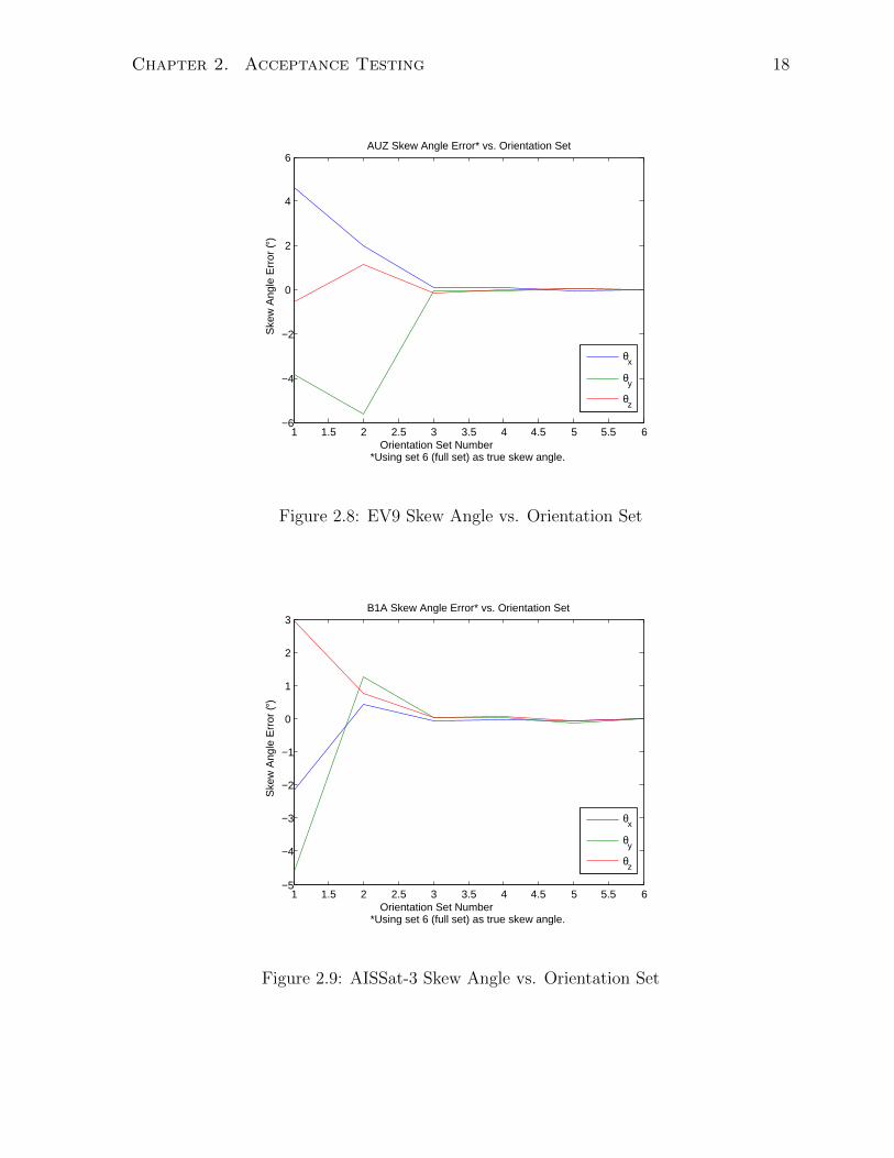
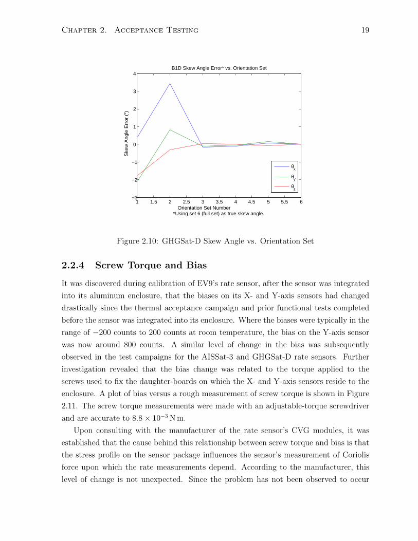
It was shown that the duration of the test could be significantly reduced while achiev-
ing similar results using fewer orientations. Calibrations were performed using 12, 9, 6,
and 3 orientations by removing intermediate orientations from the original set of 21. The
difference in the resulting scale factors and misalignment (skew) angles for three rate
sensors with serial numbers AUZ, B1A, and B1D are shown in Figures 2.5 to 2.7 and
Figures 2.8 to 2.10. The enumeration of the orientation sets is explained in Table 2.1.
These results indicate that Orientation Sets 3 to 6 achieve a similar level of performance
in estimating the skew angles, with rapidly diminishing return in all cases for increas-
ing the number of calibration orientations past that of Set 3. No significant change is
observed in the accuracy of estimating the scale factors for any orientation set since the
value of the scale factors is typically in the range of 200 counts·s/◦.
SetNumber
Number ofOrientations
Description
1 3 One orientation for each axis aligned with table axis2 6 As in Set 1 plus one for each axis aligned 45◦ with table axis.3 6 One for each axis aligned perpendicular with table axis, and
one for each axis aligned 45◦.4 9 As in Set 3 plus one for each axis aligned with table axis.5 12 Each axis oriented 0◦, 30◦, 60◦, and 90◦ from table axis.6 21 Full original set consisting of each axis oriented 0◦, 15◦, 30◦,
45◦, 60◦, 75◦, and 90◦ from table axis.
Table 2.1: Orientation Sets for Rate Sensor Calibration
Though Orientation Set 3 provided good performance, it was decided to use Orienta-
tion Set 4 for future rate sensor calibrations as an added measure of confidence, reducing

Chapter 2. Acceptance Testing 16
the number of mounting orientations to 9 and cutting the calibration time roughly in
half. However, although this analysis has shown that the effect of reducing the number
of orientations has had a small effect on the accuracy with which the calibration pa-
rameters are determined, the resulting impact on the satellite pointing error is not well
understood. Future work would explore the effect of reducing the number of calibration
orientations on pointing error arising from errors in determining the rate sensor’s scale
factors and axis skew angles.
1 1.5 2 2.5 3 3.5 4 4.5 5 5.5 6−0.5
0
0.5
1
1.5
2AUZ Scale Factor Error* vs. Orientation Set
Sca
le F
acto
r E
rror
(co
unt/(
° /s))
Orientation Set *Using 6 (full set) as true scale factor
sx
sy
sz
Figure 2.5: EV9 Scale Factor vs. Orientation Set
Chapter 2. Acceptance Testing 17
1 1.5 2 2.5 3 3.5 4 4.5 5 5.5 6−0.3
−0.2
−0.1
0
0.1
0.2
0.3
0.4B1A Scale Factor Error* vs. Orientation Set
Sca
le F
acto
r E
rror
(co
unt/(
° /s))
Orientation Set *Using 6 (full set) as true scale factor
sx
sy
sz
Figure 2.6: AISSat-3 Scale Factor vs. Orientation Set
1 1.5 2 2.5 3 3.5 4 4.5 5 5.5 6−0.3
−0.2
−0.1
0
0.1
0.2
0.3
0.4
0.5B1D Scale Factor Error* vs. Orientation Set
Sca
le F
acto
r E
rror
(co
unt/(
° /s))
Orientation Set *Using 6 (full set) as true scale factor
sx
sy
sz
Figure 2.7: GHGSat-D Scale Factor vs. Orientation Set
Chapter 2. Acceptance Testing 18
1 1.5 2 2.5 3 3.5 4 4.5 5 5.5 6−6
−4
−2
0
2
4
6
Orientation Set Number *Using set 6 (full set) as true skew angle.
Ske
w A
ngle
Err
or (°
)
AUZ Skew Angle Error* vs. Orientation Set
θx
θy
θz
Figure 2.8: EV9 Skew Angle vs. Orientation Set
1 1.5 2 2.5 3 3.5 4 4.5 5 5.5 6−5
−4
−3
−2
−1
0
1
2
3
Orientation Set Number *Using set 6 (full set) as true skew angle.
Ske
w A
ngle
Err
or (°
)
B1A Skew Angle Error* vs. Orientation Set
θx
θy
θz
Figure 2.9: AISSat-3 Skew Angle vs. Orientation Set
Chapter 2. Acceptance Testing 19
1 1.5 2 2.5 3 3.5 4 4.5 5 5.5 6−3
−2
−1
0
1
2
3
4
Orientation Set Number *Using set 6 (full set) as true skew angle.
Ske
w A
ngle
Err
or (°
)
B1D Skew Angle Error* vs. Orientation Set
θx
θy
θz
Figure 2.10: GHGSat-D Skew Angle vs. Orientation Set
2.2.4 Screw Torque and Bias
It was discovered during calibration of EV9’s rate sensor, after the sensor was integrated
into its aluminum enclosure, that the biases on its X- and Y-axis sensors had changed
drastically since the thermal acceptance campaign and prior functional tests completed
before the sensor was integrated into its enclosure. Where the biases were typically in the
range of −200 counts to 200 counts at room temperature, the bias on the Y-axis sensor
was now around 800 counts. A similar level of change in the bias was subsequently
observed in the test campaigns for the AISSat-3 and GHGSat-D rate sensors. Further
investigation revealed that the bias change was related to the torque applied to the
screws used to fix the daughter-boards on which the X- and Y-axis sensors reside to the
enclosure. A plot of bias versus a rough measurement of screw torque is shown in Figure
2.11. The screw torque measurements were made with an adjustable-torque screwdriver
and are accurate to 8.8× 10⁻³ N m.
Upon consulting with the manufacturer of the rate sensor’s CVG modules, it was
established that the cause behind this relationship between screw torque and bias is that
the stress profile on the sensor package influences the sensor’s measurement of Coriolis
force upon which the rate measurements depend. According to the manufacturer, this
level of change is not unexpected. Since the problem has not been observed to occur

Chapter 2. Acceptance Testing 20
0.08 0.1 0.12 0.14 0.16 0.18 0.2−940
−930
−920
−910
−900
−890
−880
−870
−860
−850
−840Y Axis Angular Rate Bias vs. Torque
Ang
ular
Rat
e ω
(co
unts
)
Screw Torque (Nm)
Figure 2.11: Screw Torque vs. Bias for Y-Axis Sensor
for the Z-axis sensor on the mother-board, whose screws are further away from the
sensor package, it was recommended that the daughter-boards be made larger in future
revisions of the rate sensor design to increase the spacing between the screws and the
sensor package, or to use adhesives to bond the daughter-boards to the enclosure.
There is no guarantee that the present mounting scheme for the rate sensor daughter-
boards does not place the X- and Y-axis CVG modules under unsafe stress levels. How-
ever, the current schedules for the four missions discussed in this thesis do not allow
sufficient time for a redesigned sensor to be implemented for those missions. Further
testing revealed that, though unusually high, the bias was relatively stable once the
sensor was integrated into its enclosure. Furthermore, other aspects of the rate sensor’s
performance appear to be unaffected, and the rate sensor was at no risk of saturating dur-
ing operation since spacecraft body rates were expected to remain well below ±10rad/s,
or approximately ±2200 counts, where the full range of the rate sensor is ±8192 counts.
Moreover, as previously explained, the EKF implemented in the attitude determination
and control flight software is capable of estimating and tracking a slowly changing bias,
and, additionally, is also capable of propagating spacecraft attitude state using actuator
inputs in place of rate sensor measurements. It was therefore decided to accept the rate
sensors for flight despite the high bias, and a recommendation was made to integrate
future sensors into their enclosures before the start of the acceptance test campaign to
ensure consistent performance throughout the campaign.

Chapter 2. Acceptance Testing 21
2.3 Fine Sun Sensors
2.3.1 Theory of Operation
Sun sensors are used to measure the direction of the Sun relative to the spacecraft. Fine
sun sensors provide a more accurate measurement of the sun direction vector relative to
the spacecraft, while coarse sun sensors provide a much rougher measurement and are
used in some space missions to point fine sun sensors. Pointing budgets for UTIAS-SFL
missions typically require fine sun sensors to be accurate to approximately 3◦ within three
standard deviations or better [12][19]. Coarse sun sensors are no longer used on UTIAS-
SFL missions, but have been implemented in the past by using solar panel currents to
determine the incident angle of the sun on each face of the satellite, which have been
observed to be accurate to about 30◦ or better.
As with the magnetometer, a single fine sun sensor measurement can only determine
a satellite’s attitude about two independent axes, leaving uncertainty about the Sun
vector, and is therefore typically used in combination with a magnetometer to provide
a full three-axis attitude solution. UTIAS-SFL’s in-house fine sun sensors measure the
sun vector using a two-dimensional complementary metal-oxide semiconductor (CMOS)
phototransistor array located underneath a pinhole lens. As light from the Sun passes
through the pinhole lens, a spot is projected onto the CMOS array below. A cross-section
of this is shown in Figure 2.12. In the figure, w is the width of the array. Given known
Incident Sunlight
CMOS Array
Pinhole
Figure 2.12: UTIAS-SFL Fine Sun Sensor Theory of Operation
values for the height of the pinhole h and the two components of the bias of the pinhole
from the center of the CMOS array b = [ bx by ]T , the location of the centroid of the
light spot c = [ cx cy ]T can be used to calculate the direction of the Sun in the sensor

Chapter 2. Acceptance Testing 22
frame, indicated by the subscript s, using
ss =1√
(b− c)T (b− c) + h2
[b− c
h
](2.5)
where ss, the sun vector has been normalized to unit length. Note that in Figure 2.12, ~b
and ~c are the bias and centroid vectors, with components in the sensor frame of b and c
as defined above, respectively. These are confined to the plane of the CMOS array, but
can in general be in any direction in that plane. A neutral density filter is placed on top
of the pinhole to attenuate the intensity of the incoming sunlight and also reduces the
intensity of most sources of stray light to nearly undetectable levels.
One of these sensors is typically placed on each face of a satellite in order to allow
measuring the sun vector in any attitude so long as the Sun is visible from the satellite’s
position in orbit. The low price of CMOS arrays in recent years has allowed sun sensors
of this type to be made relatively cheaply. Various iterations of UTIAS-SFL’s in-house
fine sun sensor have therefore been used on every UTIAS-SFL mission to date.
2.3.2 Testing Cycle
The testing cycle for fine sun sensors at UTIAS-SFL follows the general cycle identified in
Figure 1.2. This thesis contributed improvements to the sun sensor calibration procedure
in addition to performing acceptance testing for the EV9, AISSat-3, GHGSat-D, and
NORSAT-1 sun sensors.
2.3.3 Calibration Improvements
The sun sensor calibration estimates a sensor’s pinhole height and bias [24]. These
are estimated by finding the values of height and bias that minimize the angular error
between the measured sun direction and the true sun direction for a large number of
measurements across the range of the sensor field of view. This is elaborated below.
The sun sensor calibration setup is shown in Figure 2.13. Note that the size of the
rotator has been exaggerated for clarity. The sensor is mounted on a 3-axis rotating
platform and a simulated sun source is used to illuminate the sensor. Mirrors are used
to extend the distance between the light source and the sensor. The sensor is mounted
such that its Z-axis is parallel within misalignment error with the rotator roll axis. In
the rotator’s home position, when all actuator angles are set to 0◦, the rotator roll axis is
pointed toward the front of the room directly at the light source with some misalignment

Chapter 2. Acceptance Testing 23
error, the rotator yaw axis points at the ceiling, and the rotator pitch axis points to the
right side of the room, or out of the page in Figure 2.13.
Three right-handed orthogonal reference frames are defined in the figure: these are
the lab frame F i, the rotator frame F r, and the sensor frame F s. The lab frame
has its origin at the rotator’s center of rotation and remains fixed with respect to the
room. Its three axes[~i1 ~i2 ~i3
]Tcoincide with the rotator’s yaw, pitch, and roll axes,
respectively, at home position. The rotator frame also has its origin at the rotator’s
center of rotation, but remains fixed with respect to the sensor throughout the test.
Its three axes[~r1 ~r2 ~r3
]Tare a transformation of the axes of F i by the rotator’s
rotation angles in a yaw-pitch-roll, or 1-2-3, order. Finally, the sensor frame finds its
origin at the center of the CMOS array and remains fixed with respect to the sun sensor
throughout the test. Its three axes[~s1 ~s2 ~s3
]Tcoincide with the CMOS array’s X, Y,
and Z axes, respectively. Three vectors are also defined: ~ρrs, ~ρrl, and ~ρsl. The vector ~ρrs
extends from the rotator center of rotation to the sensor CMOS and stays fixed relative
to F r throughout the calibration. The vector ~ρrl extends from the rotator center of
rotation to the apparent position of the light source. This stays fixed with respect to
F i. Finally, ~ρsl is the vector from the sensor CMOS to the apparent light source. The
superscript letters r, s, and l refer to the rotator center of rotation, CMOS center, and
light source origin, respectively. Note that the size of the CMOS is considered negligible
at this scale and it is assumed that the rays of light incident across the CMOS are all
parallel to ~ρsl.
Rotator
Sensor
Mirror
Light Source (True)
Light Source (Apparent)
Mirror
Figure 2.13: Fine Sun Sensor Calibration Setup, Side View
Measurements of the vector from the sensor to the sun source ~ρsl are made across the

Chapter 2. Acceptance Testing 24
sensor field of view by holding the sensor at a series of pitch angles between 0◦ and 57◦,
which covers most of a typical sensor’s field of view. For each pitch angle, the sensor is
rotated into a series of roll angles evenly spaced between −180◦ and 180◦. A measurement
of the centroid of the projected light spot on the CMOS is made at each position and
the rotator angles are recorded. The yaw axis is held fixed at 0◦ throughout the test.
This generates concentric annuli of measured centroids spanning the field of view. The
spacing between the pitch and roll angles are chosen to get a total of 2000 roughly evenly
distributed measurement orientations.
The measurements made in each orientation throughout the test allow for the direction
of the sun vector ~ρslk to be calculated in two different ways. The subscript k refers to the
kth measurement orientation. The measured sun vector is calculated and normalized to
unit length using Equation 2.5, which naturally resolves the vector in the sensor frame.
Adding indices, Equation 2.5 can be rewritten as
ss,k =1√
(b− ck)T (b− ck) + h2
[b− ck
h
](2.6)
where (·) is used to indicate that this is the measured sun direction vector. This is similar
to how the sun direction vector is calculated on orbit. The true sun vector is calculated
by observing that ~ρsl = ~ρrl − ~ρrs, and using
ρslr,k = Cri,kρrli − ρrsr (2.7)
where ρrli and ρrsr are ~ρrl and ~ρrs resolved in the lab frame and rotator frame, respectively,
which are the frames in which the two vectors can be measured. ρslr,t is the true sun vector
resolved in the rotator frame, and Cri is the rotation matrix from the lab frame to the
rotator frame. In order to compare the measured and true sun vectors, the two must be
expressed in the same frame. The true sun vector can be expressed in the sensor frame by
applying an additional rotation from the rotator frame to the sensor frame to Equation
2.7 to get
ρsls,k = Csr
(Cri,kρ
rli + ρrsr
)(2.8)
This is then normalized to get the unit vector for the true sun direction
ss,k =ρsls,kρsls,k
(2.9)
Cri,k is obtained by composing three principal rotations in the order of the rotator’s order

Chapter 2. Acceptance Testing 25
of rotation
Cri,k =
cos θ3,k sin θ3,k 0
− sin θ3,k cos θ3,k 0
0 0 1
cos θ2,k 0 − sin θ2,k
0 1 0
sin θ2,k 0 cos θ2,k
1 0 0
0 cos θ1,k sin θ1,k
0 − sin θ1,k cos θ1,k
(2.10)
where θ1,k, θ2,k, and θ3,k correspond to the rotator yaw, pitch, and roll angles recorded
during the test, respectively. Csr can similarly be expressed as the composition of three
principal rotations in 3-2-1 order
Csr =
1 0 0
0 cosα − sinα
0 sinα cosα
cos β 0 sin β
0 1 0
− sin β 0 cos β
cos γ − sin γ 0
sin γ cos γ 0
0 0 1
(2.11)
where α, β, and γ are respectively referred to as the tip, tilt, and clock angles, which
characterize the misalignment between the sensor frame and the rotator frame and remain
constant throughout the test.
The angle between the measured and true sun vectors is obtained by taking
δk = cos−1 sTs,kss,k (2.12)
The calibration variables are then determined by finding the values that minimize the
root-mean-square (RMS) of δk
δRMS =
√√√√ 1
N
N∑k=1
δ2k (2.13)
where N is the total number of measurement orientations. A complete derivation of the
UTIAS-SFL fine sun sensor calibration method can be found in [25].
Since only the actuator angles and centroid locations are recorded during each cal-
ibration test, the pinhole height h and bias b are not the only parameters estimated
in post-processing of the calibration data. Previously, the sun sensor calibration script
also estimated the three sensor misalignment angles α, β, and γ, while ρrli and ρrsr were
hard-coded to values that reflect an estimate of these quantities made in the past [25].
The calibration, stated as an optimization problem, is therefore
{c∗, h∗, α∗, β∗, γ∗} = arg minc,h,α,β,γ
δRMS. (2.14)

Chapter 2. Acceptance Testing 26
A sample plot of the output from this calibration script from the NORSAT-1 sun sensor
calibration campaign is shown in Figure 2.14. The color map shows the residual sun
direction measurement error across the sensor field of view resulting from the optimal
pinhole height and bias values found by the script, while the red points indicate the
centroid locations measured throughout the test. The pinhole height and bias found
by the script are shown above the plot, and fall within the expected range for these
parameters. The tip, tilt, and clock angles are not shown, but were found to be α =
−0.19◦, β = −0.13◦, and γ = 266.1◦. These are also within the expected ranges, with
the tip and tilt angles being small and the clock angle corresponding roughly to a 3/4
rotation about the rotator frame roll axis, which is how the sensor was mounted. The
full accuracy and inner 90% accuracy displayed above the plot refer to the root mean
square (RMS) error of the whole field of view and the inner 90% of the field of view,
respectively. These results suggest that the RMS accuracy of the sensor is 0.35◦ within
the inner 90% of the field of view.
Figure 2.14: Calibration Results, ρrli and ρrsr Hard-Coded
However, on-orbit performance of the sun sensors calibrated using this procedure has

Chapter 2. Acceptance Testing 27
shown that this accuracy is not being achieved, and that the actual accuracy is typically
around 2◦. This is shown using on-orbit data from one of the BRITE satellites in Figure
2.15. The angle between the sun direction measured by a sun sensor and that predicted
based on the star tracker attitude, which is considered much more accurate than the
sun sensor, are shown from both on-orbit data and a simulation. One suggested reason
Figure 2.15: On Orbit vs. Simulated Sun Sensor Error
for this discrepancy was that the values of ρrli and ρrsr implemented in the script were
wrong, possibly due to changes in the setup geometry since the values were measured.
It was therefore decided to investigate the possibility of estimating ρrli and ρrsr together
with the pinhole height and bias and sensor misalignment angles using the same data.
If successful, this would improve the accuracy of sun sensors flying on satellites that are
already on-orbit without recalibrating.
Estimating ρrli and ρrsr amounts to estimating the geometry of the triangle formed
by ~ρsl, ~ρrl, and ~ρrs. In general, this would be defined by 6 independent parameters.
However, since the calibration works with unit vectors for the sun direction, the true
lengths of the sides of this triangle are ignored by the calibration routine, which removes

Chapter 2. Acceptance Testing 28
one independent parameter. It was therefore decided to enforce ~ρrl to be unit length.
This constraint was enforced by defining a new frame F l and a new rotation matrix
Cil , ~F i · ~FT
l . F l shares an origin with F i at the rotator center of rotation and its axes
are such that ~l3 is colinear with ~ρrl, ~l2 lies in the plane defined by ~ρrl and ~i3, between
~ρrl and ~i3, and ~l1 completes the right-handed orthogonal triad. The components of ~ρrl
in F l are then simply ρrll =[
0 0 1]T
. The rotation between F l and F i can then be
expressed as a composition of two principal rotations, first about ~l1, and then about the
third axis of the intermediate frame so that
Cil =
cosφ − sinφ 0
sinφ cosφ 0
0 0 1
1 0 0
0 cosλ − sinλ
0 sinλ cosλ
(2.15)
This guarantees that the resulting vector estimated in F i is of unit length. The newly
added parameters to be estimated are therefore φ, λ, and the three components of ρrsr ,
corresponding to the 5 independent parameters that define the triangle described earlier.
The optimization problem for the calibration thus becomes
{c∗, h∗, α∗, β∗, γ∗, φ∗, λ∗,ρrsr∗} = arg min
c,h,α,β,γ,φ,λ,ρrsrδRMS. (2.16)
The output from the modified calibration routine is shown in Figure 2.16. The plot
shows that the residual error has been highly reduced, with the RMS error for the
inner 90% of the field of view roughly halved. Moreover, the error in the higher er-
ror regions near the edge of the field of view has been drastically reduced. However,
the pinhole height falls far outside of the expected range of 1 mm ± 0.1 mm that has
been observed for all past calibrations of identical sensors, including those performed
with an older setup that produced good results. The calibration also estimated that
ρrsr =[
0.00077 −0.0050 −0.28]T
, which suggests that ~ρrs is nearly one third of the
length of ~ρrl, where in reality this fraction should be an order of magnitude smaller. The
true length of ~ρrl is on the order of a few meters, whereas the true length of ~ρrs is just
a few centimeters. However, λ and φ were found to be 1.53◦ and 44.2◦, both believable
values. There was no appreciable change in the tip, tilt, and clock angles.
Given the unrealistic estimates of the pinhole height and the rotator-sensor vector,
these results are not expected to provide accurate measurement of the sun direction vector
on-orbit despite what the residual error plot might suggest, showing that there is still a an
error in the updated calibration method. It was found through further experimentation
that constraining the third component of ρrsr to fall within 0±0.1 resulted in an estimate

Chapter 2. Acceptance Testing 29
Figure 2.16: Calibration Results, ρrli and ρrsr Estimated
of −0.1, but the RMS accuracy would be degraded, with the higher error regions around
the edge of the field of view becoming visible once again. The estimated pinhole height
would also be reduced. Fixing the third component of ρrsr to a value closer to 0 would
result in a further reduction in the RMS accuracy and a proportional increase in the
pinhole height. There was no appreciable difference observed in the other parameters.
It appears, therefore, that the degree of freedom introduced by adding ρrsr allows the
optimizer to falsely compensate for an unmodeled effect at the edge of the field of view,
with an accompanying change in the pinhole height.
More work is needed in order to understand and address this problem. One possible
approach is to measure the true values of ρrsr and ρrli and hard-code them into the cali-
bration script. This is, as was the previous version of the calibration routine, susceptible
to changes in the test setup and measurement error. Another approach, more preferable,
is to run the optimization on data collected for a smaller portion of the field of view. The
challenge with this approach is in deciding how much of the field of view to exclude, and
would require further study of the problem to understand the nature of the unmodeled

Chapter 2. Acceptance Testing 30
effect. In either case, validation of the calibration can be performed by comparing to
results from an on-orbit calibration of the fine sun sensors on the BRITE mission.
2.4 Reaction Wheels
2.4.1 Theory of Operation
Reaction wheels are used to control a spacecraft’s attitude by transferring angular mo-
mentum between the wheels and the rest of the spacecraft. A reaction wheel consists of
a rotor of known moment of inertia spun by a motor about a single axis. Three reaction
wheels are mounted orthogonally to the satellite bus for UTIAS-SFL satellites in order
to provide control on three independent axes. The dynamics of a spacecraft with three
reaction wheels expressed in some reference frame F b fixed to the spacecraft body and
centered at the center of mass is governed by [26]
Ibωb + ω×b Ibωb + IsAbωs + ωb×IsAbωs = Gb, (2.17)
where Ib is the satellite moment of inertia, ωb is the satellite angular velocity, Is is the
reaction wheel moment of inertia, and Gb is the sum of the remaining torques on the
satellite. The elements of ωs =[ωs,1 ωs,2 ωs,3
]Tare the rates of rotation, or wheel
speeds, of each reaction wheel, with each column ab,j ofAb containing the rotation axis of
the corresponding wheel. The term Isωs,j is sometimes referred to as the wheel “torque”.
Note, though, that this does not correspond to the total torque applied by the wheel to
the satellite since it ignores the gyric term ωb×Isωs,jab,j. On UTIAS-SFL satellites, the
wheel speed is measured by differentiating output from a Hall effect encoder. Two sizes
of wheel are used. The smaller model can sustain a maximum Isωs = 30 mN m s and
has a moment of inertia of Is = 5.12× 10⁻⁵ kg m2. These are standard on the Generic
Nanosatellite Bus platform and are used by AISSat-3 and EV9. The larger model can
sustain Isωs = 60 mN m s and has a moment of inertia Is = 8.78× 10⁻⁵ kg m2. These are
standard on the NEMO bus platform and are used by GHGSat-D and NORSAT-1. The
reaction wheel axes are usually aligned with the satellite axes, such that Ab is usually
treated as simply the 3 × 3 identity matrix, though in reality there is also a mounting
misalignment, which is budgeted for in the mission pointing budget.
The attitude control system for UTIAS-SFL satellites is, in theory, a zero-momentum
system, meaning that the wheels are nominally non-spinning when the satellite is held
fixed relative to inertial space. However, in practice, each wheel is set to track 50 rad/s
Chapter 2. Acceptance Testing 31
while idling in order to avoid operating in the zero-crossing range where wheel speed
measurement accuracy is poor due to less frequent encoder output. A spacecraft will
also gradually accumulate angular momentum in orbit due to the action of disturbance
torques. This angular momentum must be absorbed by the wheels and eventually re-
moved from the spacecraft to avoid saturating the wheels. For this reason, UTIAS-SFL
satellites are augmented with magnetic torquers, or magnetorquers, as secondary actua-
tors to continuously dump angular momentum as it is absorbed.
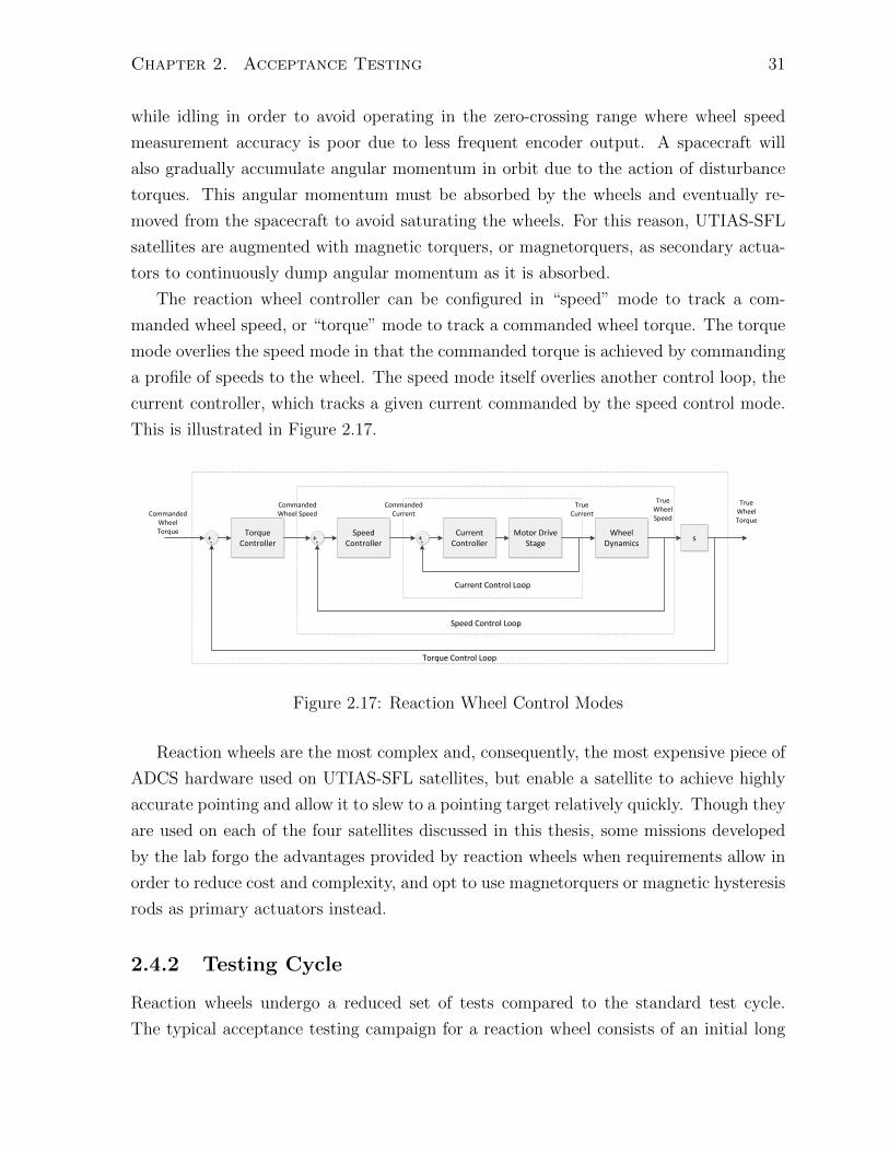
The reaction wheel controller can be configured in “speed” mode to track a com-
manded wheel speed, or “torque” mode to track a commanded wheel torque. The torque
mode overlies the speed mode in that the commanded torque is achieved by commanding
a profile of speeds to the wheel. The speed mode itself overlies another control loop, the
current controller, which tracks a given current commanded by the speed control mode.
This is illustrated in Figure 2.17.
-Wheel
DynamicsMotor Drive
Stages
Current Control LoopCurrent Control Loop
+-+- +
Speed Control LoopSpeed Control Loop
Torque Control LoopTorque Control Loop
TrueWheelTorque
TrueWheelSpeed
True Current
CommandedCurrent
CommandedWheel SpeedCommanded
WheelTorque Current
ControllerSpeed
ControllerTorque
Controller
Figure 2.17: Reaction Wheel Control Modes
Reaction wheels are the most complex and, consequently, the most expensive piece of
ADCS hardware used on UTIAS-SFL satellites, but enable a satellite to achieve highly
accurate pointing and allow it to slew to a pointing target relatively quickly. Though they
are used on each of the four satellites discussed in this thesis, some missions developed
by the lab forgo the advantages provided by reaction wheels when requirements allow in
order to reduce cost and complexity, and opt to use magnetorquers or magnetic hysteresis
rods as primary actuators instead.
2.4.2 Testing Cycle
Reaction wheels undergo a reduced set of tests compared to the standard test cycle.
The typical acceptance testing campaign for a reaction wheel consists of an initial long

Chapter 2. Acceptance Testing 32
form functional test (LFFT), a thermal acceptance campaign, and a closeout LFFT. The
LFFT for a reaction wheel consists of a built-in short form functional test (SFFT), a
torque tracking error test, a noise over speed test, and a power consumption over speed
test. The wheels are delivered by the manufacturer as an assembled unit, and T-shock
testing is handled by the manufacturer.
This thesis contributed improvements to the torque error test, investigated issues with
timestamping in wheel test results, and assessed the effect of a current sensor bias on the
EV9 and AISSat-3 wheels.
2.4.3 Torque Test Improvements
The purpose of the torque test is to measure a reaction wheel’s performance in tracking
torque commands at various speeds. The reaction wheel is commanded to hold a certain
speed, and then issued a torque command. Wheel speed measurements are collected for
one minute while the torque is being applied. This is repeated for other combinations
of wheel speeds and torques. The particular speeds and torques are notionally chosen to
reflect mission requirements, but in practice are standardized for the 30 mNms wheels
and the 60 mNms wheels. In either case, the speeds consist of a low speed and a high
speed, and the torques similarly consist of a low torque and a high torque. The low
torques are chosen to be roughly representative of the torque required for nadir tracking,
while the high torque is chosen to be reflective of the torque needed for slewing. The
low speed is chosen as the idle speed of the wheels, reflecting the wheel speed at the
beginning of a maneuver, and the high speed is chosen as the highest speed expected
for the wheels during a slew, reflecting the wheel speed mid-maneuver. Previously, the
low and high torques were applied in both the negative and positive directions, but
only positive speeds were tested, giving a total of eight speed and torque combinations.
However, it was decided that both negative and positive speeds should be included for
completeness to give a new total of 16 cases. Table 2.2 gives the values of low and high
speed and torque used for the 30 mNms wheels and the 60 mNms wheels.
30 mNms 60 mNms
Low Speed (rad/s) 100 50High Speed (rad/s) 300 300Low Torque (Nm) 10−6 10−5
High Torque (Nm) 4× 10⁻⁴ 6× 10⁻⁵
Table 2.2: Reaction Wheel Torque Test Speeds and Torques
Chapter 2. Acceptance Testing 33
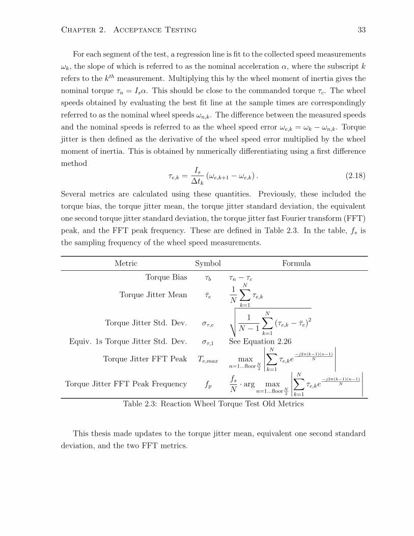
For each segment of the test, a regression line is fit to the collected speed measurements
ωk, the slope of which is referred to as the nominal acceleration α, where the subscript k
refers to the kth measurement. Multiplying this by the wheel moment of inertia gives the
nominal torque τn = Isα. This should be close to the commanded torque τc. The wheel
speeds obtained by evaluating the best fit line at the sample times are correspondingly
referred to as the nominal wheel speeds ωn,k. The difference between the measured speeds
and the nominal speeds is referred to as the wheel speed error ωe,k = ωk − ωn,k. Torque
jitter is then defined as the derivative of the wheel speed error multiplied by the wheel
moment of inertia. This is obtained by numerically differentiating using a first difference
method
τe,k =Is
∆tk(ωe,k+1 − ωe,k) . (2.18)
Several metrics are calculated using these quantities. Previously, these included the
torque bias, the torque jitter mean, the torque jitter standard deviation, the equivalent
one second torque jitter standard deviation, the torque jitter fast Fourier transform (FFT)
peak, and the FFT peak frequency. These are defined in Table 2.3. In the table, fs is
the sampling frequency of the wheel speed measurements.
Metric Symbol Formula
Torque Bias τb τn − τc
Torque Jitter Mean τe1
N
N∑k=1
τe,k
Torque Jitter Std. Dev. στ,e
√√√√ 1
N − 1
N∑k=1
(τe,k − τe)2
Equiv. 1s Torque Jitter Std. Dev. στ,1 See Equation 2.26
Torque Jitter FFT Peak Te,max maxn=1...floorN
2
∣∣∣∣∣N∑k=1
τe,ke−j2π(k−1)(n−1)
N
∣∣∣∣∣Torque Jitter FFT Peak Frequency fp
fsN· arg max
n=1...floorN2
∣∣∣∣∣N∑k=1
τe,ke−j2π(k−1)(n−1)
N
∣∣∣∣∣Table 2.3: Reaction Wheel Torque Test Old Metrics
This thesis made updates to the torque jitter mean, equivalent one second standard
deviation, and the two FFT metrics.

Chapter 2. Acceptance Testing 34
Torque Jitter Mean
The purpose of the torque jitter mean metric was to measure the mean deviation of
the applied torque from the nominal torque [27]. The intent was to detect long-period
drifts from the nominal torque. However, it was discovered that this metric was only
reflective of the difference between the first wheel speed measurement and final wheel
speed measurement as well as the total measurement duration in each test segment, and
was therefore not a meaningful metric. This result can be shown by first substituting
Equation 2.18 into the formula for torque jitter mean in Table 2.3
τe =IsN
N∑k=1
1
∆tk(ωe,k+1 − ωe,k) (2.19)
Usually, ∆tk = ∆tl = ∆t ∀k, l, i.e. the sampling interval is uniform. Substituting in the
definition of ωe,k gives
τe =IsN∆t
N∑k=1
(ωk+1 − ωn,k+1 − ωk + ωn,k) (2.20)
=IsN∆t
N∑k=1
(ωk+1 − ωk)−IsN∆t
N∑k=1
(ωn,k+1 − ωn,k) . (2.21)
Working with the second term, in Equation 2.21, we find
IsN∆t
N∑k=1
(ωn,k+1 − ωn,k) =IsN
N∑k=1
α = Isα = τn. (2.22)
Now working with the first term in Equation 2.21, the middle terms in the summation
cancel and the summation collapses into
N∑k=1
(ωk+1 − ωk) = ωN+1 − ω1. (2.23)
Finally, substituting Equations 2.22 and 2.23 into Equation 2.21 gives
τe =Is (ωN+1 − ω1)
N∆t− τn, (2.24)
which contains no information about the data between the first and last wheel speed
measurements.
It was decided to replace this metric with the coefficient of determination, or R-

Chapter 2. Acceptance Testing 35
squared value, of the regression line fitted through the wheel speed measurements. This
serves the original intent of the torque jitter mean to detect long-period drifts, since
these drifts would also be apparent in the wheel speed measurements and be reflected
by a lower R-squared value, indicating a poor fit. Further work is needed to validate the
efficacy of this metric in detecting real long-period drifts.
One-Second Equivalent Torque Jitter Standard Deviation
The one second equivalent standard deviation metric is used in Mirage, UTIAS-SFL’s in-
house satellite attitude simulator, as the standard deviation of an additive white Gaussian
source of torque noise. Using this standard deviation, the noise source should, when
sampled at the simulation update frequency, generate torque noise that has a similar
effect on spacecraft pointing as the torque jitter measured in the torque test. For Mirage,
the simulation update frequency is 1 Hz. The usual torque jitter standard deviation
στ,e could not be used to define the noise source because aliasing results in larger-than-
expected pointing error on the next cycle.
Previously, the approach used to calculate this metric was to first partition the torque
jitter into M one-second segments, where M =⌊N∆t
1s
⌋and calculate the means of each
segment
τe,l =1
Nl+1 −Nl
Nl+1−1∑k=Nl
τe,k (2.25)
where l indicates the lth segment and Nl refers to the index of the first point in the lth
segment. The one-second equivalent standard deviation is then the standard deviation
of these means
στ,1 =
√√√√ 1
M − 1
M∑l=1
(τe,l −
1
M
M∑l=1
τe,l
)2
. (2.26)
στ,1 usually has values on the order of 10−6, which is much lower than στ,e, which typically
has values on the order of 10−4, as desired. This seems intuitively to be a valid approach,
but it was never shown that this would result in a noise source that would accurately
reflect the measured torque jitter, and it was suspected that this approach produced
results that are too optimistic. A more rigorous approach to this metric was desired.
One approach that was considered was to apply an anti-aliasing filter to the signal and
calculate the standard deviation of the filtered signal. The anti-aliasing filter is simply
an ideal low-pass filter with a cutoff frequency of 0.5 Hz, or one half the sampling rate.
The filtered signal is calculated by taking its convolution with the anti-aliasing filter. In
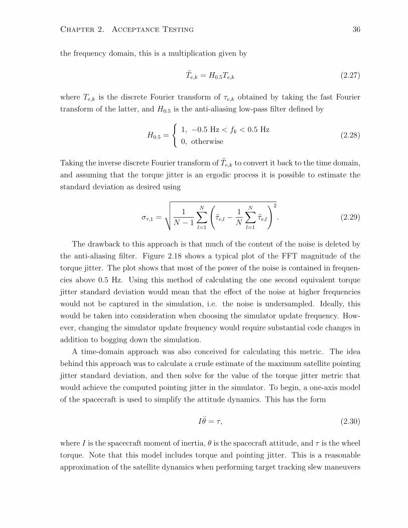
Chapter 2. Acceptance Testing 36
the frequency domain, this is a multiplication given by
Te,k = H0.5Te,k (2.27)
where Te,k is the discrete Fourier transform of τe,k obtained by taking the fast Fourier
transform of the latter, and H0.5 is the anti-aliasing low-pass filter defined by
H0.5 =
{1, −0.5 Hz < fk < 0.5 Hz
0, otherwise(2.28)
Taking the inverse discrete Fourier transform of Te,k to convert it back to the time domain,
and assuming that the torque jitter is an ergodic process it is possible to estimate the
standard deviation as desired using
στ,1 =
√√√√ 1
N − 1
N∑l=1
(τe,l −
1
N
N∑l=1
τe,l
)2
. (2.29)
The drawback to this approach is that much of the content of the noise is deleted by
the anti-aliasing filter. Figure 2.18 shows a typical plot of the FFT magnitude of the
torque jitter. The plot shows that most of the power of the noise is contained in frequen-
cies above 0.5 Hz. Using this method of calculating the one second equivalent torque
jitter standard deviation would mean that the effect of the noise at higher frequencies
would not be captured in the simulation, i.e. the noise is undersampled. Ideally, this
would be taken into consideration when choosing the simulator update frequency. How-
ever, changing the simulator update frequency would require substantial code changes in
addition to bogging down the simulation.
A time-domain approach was also conceived for calculating this metric. The idea
behind this approach was to calculate a crude estimate of the maximum satellite pointing
jitter standard deviation, and then solve for the value of the torque jitter metric that
would achieve the computed pointing jitter in the simulator. To begin, a one-axis model
of the spacecraft is used to simplify the attitude dynamics. This has the form
Iθ = τ, (2.30)
where I is the spacecraft moment of inertia, θ is the spacecraft attitude, and τ is the wheel
torque. Note that this model includes torque and pointing jitter. This is a reasonable
approximation of the satellite dynamics when performing target tracking slew maneuvers

Chapter 2. Acceptance Testing 37
0 5 10 15 20 250
0.5
1
1.5
2
2.5x 10
−5Torque Jitter Single−Sided Amplitude Spectrum of Wheel: 60−171 at 48HzParsing of commanded torque 1×10⁻⁵ Nm at 300 rad/s completed.
Frequency (Hz)
Tor
que
Jitte
r A
mpl
itude
(N
m/√H
z)
Figure 2.18: Reaction Wheel Torque Jitter FFT
during which the satellite only slews about one axis. The nominal jitter free dynamics
are given by
Iθn = τn, (2.31)
where θn and τn are the nominal spacecraft attitude and wheel torque, respectively.
Subtracting Equation 2.31 from Equation 2.30 gives the jitter dynamics
I(θ − θn
)= τ − τn (2.32)
Iθe = τe. (2.33)
Here, θe and τe are the pointing and torque jitter, respectively. Integrating Equation 2.33
twice over one-second segments and dividing by the moment of inertia gives the pointing
jitter over each segment
θe,l =1
I
∫ tl+1
tl
∫ t′
tl
τedtdt′. (2.34)
This can be related to the one-second equivalent torque jitter τe,1,l by observing that the
latter is treated by the simulator as a zero-order hold, represented here by τe,1 as it is

Chapter 2. Acceptance Testing 38
propagated through the attitude dynamics. It is desired that the values of τe,1 satisfy
θe,l =1
I
∫ tl+1
tl
∫ t′
tl
τe,1dtdt′. (2.35)
Since τe,1 is a zero-order hold of a 1 Hz discrete-time signal, it is constant over one-second
intervals. Thus,
θe,l =τe,1,1I
∫ tl+1
tl
∫ t′
tl
dtdt′ (2.36)
=τe,1∆t2
2I(2.37)
where ∆t = tk+1 − tk.Taking the standard deviation of θe,l gives
σθ,1,l =√⟨
θ2e,l
⟩− 〈θe,l〉2 (2.38)
where 〈·〉 is the expected value operator. Assuming the pointing jitter is ergodic, σθ,1,l =
σθ,1,m = σθ,1 ∀l,m. Substituting in Equation 2.37 gives
σθ,1 =
√√√√⟨(τe,1,l∆t22I
)2⟩−⟨τe,1,l∆t2
2I
⟩2
(2.39)
=
√∆t4
4I2
(⟨τ 2e,1,l
⟩− 〈τe,1,l〉2
)(2.40)
=∆t2
2I
√⟨τ 2e,1,l
⟩− 〈τe,1,l〉2 (2.41)
=∆t2
2Iστ,1 (2.42)
which can be rearranged to get
στ,1 =2I
∆t2σθ,1. (2.43)
In practice, using discrete data and again assuming the pointing jitter is ergodic, θe,l
is calculated from the wheel torque measurements by trapezoidal integration
θe,l =1
I
kl+1−1∑k′=kl
∆t′k2
(k′+1∑k=kl
∆tk (τe,k+1 + τe,k)
2+
k′∑k=kl
∆tk (τe,k+1 + τe,k)
2
)(2.44)

Chapter 2. Acceptance Testing 39
and σθ,1 is estimated using
σθ,1 =
√√√√ 1
M − 1
M∑l=1
(θe,l −
1
M
M∑l=1
θe,l
)2
. (2.45)
where M is the total number of one-second intervals. The axial moments of inertia of
the spacecraft are used for I in order to produce an estimate of the metric for each axis.
This method is similar to the old method of Equation 2.26, the key difference being
that the torque signal is integrated twice rather than just once. The advantage of this
method is that it attempts to capture the effect of the torque jitter on the spacecraft
pointing jitter. Additionally, by substituting the allowable pointing jitter from the mis-
sion requirements as σθ,1 into Equation 2.43, a rough estimate of the required one-second
equivalent torque jitter of the wheels can be calculated and compared to the value cal-
culated from measurements as a quick check of a wheel’s performance. However, this
method relies on approximate numerical integration of the torque jitter to estimate the
pointing jitter, and also neglects the effects of gyric torques since it relies on a one-axis
model.
A third method conceived for calculating the metric arrives at a new model for gen-
erating torque noise in Mirage rather than a formula for calculating the existing metric.
This method approaches the conversion between the standard deviation of the measured
torque jitter to an equivalent one-second torque jitter standard deviation as a discretiza-
tion problem. As with the previous approach, this method uses a single-axis model for
spacecraft attitude dynamics but with variables defined differently. Here, the model is
constructed with the form
Iθ = u+ w (2.46)
where I is again the spacecraft moment of inertia, θ is the spacecraft attitude, u is the
applied wheel torque, and w is the wheel torque jitter. w is assumed to be an additive
white Gaussian noise source, i.e.
w ∼ N (0, στ,e) , 〈w(t)w(t′)〉 = 0 ∀t 6= t′ (2.47)
where στ,e is the usual torque jitter standard deviation as defined in Table 2.3.
Defining a state x =[x1 x2
]so that x1 , θ and x2 , θ and output y = θ,

Chapter 2. Acceptance Testing 40
Equation 2.46 can be written in state-space form
˙[x1
x2
]=
[0 1
0 0
]︸ ︷︷ ︸
A
[x1
x2
]+
[01I
]︸ ︷︷ ︸B
u+
[01I
]︸ ︷︷ ︸E
w (2.48)
y =[
1 0]
︸ ︷︷ ︸C
x (2.49)
Multiplying both sides of Equation 2.48 by e−At gives
e−Atx = e−AtAx+ e−AtBu+ e−AtEw (2.50)
Now, moving the first term on the right side of Equation 2.50 to the left side, then
integrating over the sample period T ,∫ tk+T
tk
(e−Atx− e−AtAx
)dt =
∫ tk+T
tk
e−At (Bu+Ew) dt (2.51)
e−A(tk+T )xk+1 = e−A(tk)xk +
∫ tk+T
tk
e−At (Bu+Ew) dt (2.52)
xk+1 = eATxk +
∫ tk+T
tk
eA(tk+T−t) (Bu+Ew) dt (2.53)
where xk = x(tk). Now making a change of variables so that
τ = tk + T − t, dτ = −dt, (2.54)
Equation 2.53 becomes
xk+1 = eATxk +
∫ T
0
eAτ (Bu+Ew) dτ. (2.55)
The commanded torque u remains constant over each control cycle. The control cycle
also has a period of one second, which means that u remains constant over the integration
period and may be factored out of the integral
xk+1 = eATxk +
∫ T
0
eAτdτBuk +
∫ T
0
eAτEwdτ (2.56)
Chapter 2. Acceptance Testing 41
where uk = u(tk). Now,
eAT =
[1 T
0 1
](2.57)
and ∫ T
0
eAτdτ =
∫ T
0
[1 τ
0 1
]dτ =
[T T 2
2
0 T
](2.58)
Dealing with the second integral term in Equation 2.56 is more involved due to the
integration of a random variable. However, this can be simplified by treating the entire
term as a random variable wk with covariance
QT =
⟨(∫ T
0
eAτEwdτ
)(∫ T
0
eAτEwdτ
)T⟩(2.59)
Combining the two integrals gives
QT =
⟨∫ T
0
∫ T
0
eAτEw(τ)w(τ ′)ET eAT τdτdτ ′
⟩(2.60)
The order of the integral and the expectation can be switched since the expectation
operator is an ensemble average, whereas the integration is over the time domain, getting
QT =
∫ T
0
∫ T
0
eAτE 〈w(τ)w(τ ′)〉ET eAT τ ′dτdτ ′ (2.61)
However,
〈w(τ)w(τ ′)〉 =
{0, τ 6= τ ′
σ2τ,e, τ = τ ′
(2.62)
Equation 2.61 thus becomes
QT = σ2τ,e
∫ T
0
eAτEET eAT τdτ (2.63)
= σ2τ,e
∫ T
0
[1 τ
0 1
][0 0
0 1I2
][1 0
τ 1
]dτ (2.64)
= σ2τ,e
[T 3
3I2T 2
2I2
T 2
2I2TI2
](2.65)
Substituting Equations 2.57, 2.58, and 2.65 into Equation 2.56, it is possible to write the

Chapter 2. Acceptance Testing 42
discretized state space equations[x1,k+1
x2,k+1
]=
[1 T
0 1
][x1,k
x2,k
]+
[T T 2
2
0 T
][01I
]uk +
[w1,k
w2,k
](2.66)
=
[1 T
0 1
]︸ ︷︷ ︸
Ad
[x1,k
x2,k
]+
[T 2
2ITI
]︸ ︷︷ ︸Bd
uk +
[w1,k
w2,k
](2.67)
yk =[
1 0]
︸ ︷︷ ︸Cd
xk (2.68)
where [w1,k
w2,k
]∼ N
(0, σ2
τ,e
[T 3
3I2T 2
2I2
T 2
2I2TI2
])(2.69)
Note that, under the one-axis model for spacecraft attitude dynamics, Equations 2.67
and 2.68 are the exact discretized forms of Equations 2.48 and 2.49, i.e. the solution of
Equations 2.67 and 2.68 satisfy xk = x (tk) ∀k.
In order to express the equivalent one-second wheel torque jitter in a form that can
be used in Mirage, Equations 2.67 and 2.68 must be converted into a single difference
equation. To do this, first take z transforms of both sides to get
zX (z) = AdX (z) +BdX (z) +W (z) (2.70)
Y (z) = CdX (z) . (2.71)
Rearranging and solving for Y as a function of U and W ,
(z1−Ad)X (z) = BdU (z) +W (z) (2.72)
X (z) = (z1−Ad)−1BdU (z) + (z1−Ad)
−1W (z) (2.73)
Y (z) = Cd (z1−Ad)−1BdU (z) +Cd (z1−Ad)
−1W (z) (2.74)
where 1 is the identity matrix. Now,
z1−Ad =
[z − 1 −T
0 z − 1
](2.75)

Chapter 2. Acceptance Testing 43
(z1−Ad)−1 =
[z − 1 T
0 z − 1
]∣∣∣∣∣ z − 1 −T
0 z − 1
∣∣∣∣∣=
1
(z − 1)2
[z − 1 T
0 z − 1
](2.76)
Substituting Equation 2.76 back into Equation 2.74,
Y (z) =1
(z − 1)2
([1 0
] [ z − 1 T
0 z − 1
][T 2
2ITI
]U (z)
+[
1 0] [ z − 1 T
0 z − 1
]W (z)
) (2.77)
Rearranging eventually leads to
z2Y (z)− 2zY (z) + Y (z) =T 2
2IzU (z) +
T 2
2IU (z) + zW1 (z)−W1 (z) + TW2 (z) (2.78)
Taking the inverse z transform gives
yk+2 − 2yk+1 + yk =T 2
2Iuk+1 +
T 2
2Iuk + w1,k+1 − w1,k + Tw2,k, (2.79)
and rearranging to convert back into units of torque, as well as substituting back θ in
place of y,
I
T 2(θk+2 − 2θk+1 + θk) =
1
2uk+1 +
1
2uk + w1,k+1 − w1,k +
w2,k
T, (2.80)
where wk = IT 2wk with [
w1,k
w2,k
]∼ N
(0, σ2
τ,e
[1
3T1
2T 2
12T 2
1T 3
])(2.81)
The last three terms of Equation 2.80 can be added to the nominal wheel torque in
Mirage to generate torque jitter, and constitute the terms of the new torque model. The
covariances of these terms are calculated using the standard deviation of the measured
torque jitter and scaled by the sampling time. This model suggests that an accurate
discrete torque jitter model requires two statistically dependent Gaussian white noise
sources rather than a single noise source.
This approach of modeling the torque jitter is the most rigorous of the three discussed
in this section. The only simplification made in deriving the model is the use of one-axis

Chapter 2. Acceptance Testing 44
attitude dynamics. However, further work is needed to validate this model and compare
its performance against the others, as well as against the previous method of averaging
the torque jitter. This would involve implementing each of these methods in Mirage
and comparing the simulation results against real on-orbit data collected under the same
pointing conditions. Unfortunately, the time available for this thesis was insufficient to
complete this work due to more mission-critical hardware testing taking higher priority.
Fast-Fourier Transform Area
During the acceptance testing campaigns for the NORSAT-1 and GHGSat-D reaction
wheels, a low-frequency spike was observed in the torque jitter FFT magnitude plots
for the low-speed torque test cases. An example of this is shown in Figure 2.19. Such
low-frequency spikes indicate the presence of a low-frequency oscillation in the reaction
wheel torque jitter, which could have a noticeable impact on the satellite’s pointing
performance.
0 5 10 15 20 25 30 35 40 45 500
1
2
3
4
5
6
7
8x 10
−6Torque Jitter Single−Sided Amplitude Spectrum of Wheel: 60−173 at 97HzParsing of commanded torque 1×10⁻⁵ Nm at 50 rad/s completed.
Frequency (Hz)
Tor
que
Jitte
r A
mpl
itude
(N
m/√H
z)
Figure 2.19: Torque Jitter FFT Spike on NORSAT-1 Reaction Wheel
These spikes were only detected upon reviewing the plots generated by the test anal-

Chapter 2. Acceptance Testing 45
ysis script. Due to the large number of plots generated by the script, reviewing them is
a labor-intensive process. In order to help automate the detection of these torque jitter
FFT spikes, it was decided that an estimate of the area under the FFT plot up to 10 Hz
would be added to the torque test analysis. Since the magnitude of the Fourier transform
is the square root of the power spectral density (PSD) of a signal, this gives an estimate
of the power of the torque jitter up to 10 Hz. The cutoff frequency of 10 Hz was chosen
because the spacecraft attitude dynamics act as a low-pass filter, reducing the impact of
torque jitter at higher frequencies.
The area under the FFT magnitude plot is calculated by applying a trapezoidal
integration rule to the torque jitter FFT magnitude, i.e.
A =kc−1∑k=1
∆fk(Te,k+1 − Te,k)
2(2.82)
where fkc = 10 Hz. This calculation was validated by comparing reaction wheel test data
from the earlier NEMO-AM and NEMO-HD missions, which showed even larger spikes,
to GHGSat-D and NORSAT-1 data. A plot of the torque jitter FFT magnitude from a
NEMO-HD reaction wheel is shown in Figure 2.20. The FFT area for NEMO-HD and
NEMO-AM wheels was found to be typically on the order of 3×10⁻⁵ whereas that for the
NORSAT-1 and GHGSat-D wheels was found to be around 8× 10⁻⁶. Using GHGSat-D
mass properties, analysis has shown that the corresponding overall contributions of these
spikes to the pointing error are 2.5 × 10⁻³ ◦ and 7.5 × 10⁻⁴ ◦, respectively, which are
negligible compared to the overall pointing error of 0.14◦ allocated to the reaction wheels
in the pointing budget [12]. However, further work is needed in order to determine an
acceptance criterion for this metric, since the relationship between the FFT area and the
impact on pointing error is not straightforward. As an interim measure, future wheels
tested with this metric will be compared to results obtained with past wheels, with further
analysis being performed as necessary if it is found that any future wheels perform worse.
2.4.4 Timestamp Uniformity
The reaction wheel torque test was previously run twice in each LFFT: once with a
polling rate of 20 Hz and once with a polling rate of 60 Hz. The purpose of this was to
determine if any anomalies seen in the results were artifacts of poor timestamping. It
has been observed that the 60 Hz test often produces results with inaccurate or duplicate
timestamps, which substantially degrades the results. Although the 20 Hz test usually

Chapter 2. Acceptance Testing 46
0 5 10 15 20 25 30 350
0.5
1
1.5
2
2.5
3x 10
−5Torque Jitter Single−Sided Amplitude Spectrum of Wheel: 60−141 at 64Hz
Parsing of commanded torque 6×10⁻⁵ Nm at 50 rad/s completed.
Frequency (Hz)
Tor
que
Jitte
r A
mpl
itude
(N
m/√H
z)
Figure 2.20: Torque Jitter FFT Spike on NEMO-HD Reaction Wheel
produces relatively uniform timestamps, the low sampling rate results in aliasing that
makes it impossible to distinguish between low-frequency torque jitter anomalies that
could affect the satellite’s pointing performance and high-frequency anomalies that would
be filtered out by the spacecraft’s attitude dynamics. A plot of the delta times, or time
steps, between each timestamp for one segment of a 60 Hz torque test is shown in Figure
2.21.
Updates to UTIAS-SFL’s wheel interface software, WheelTerm, were attempted,
which substantially improved the consistency of the timestamps for high poll rates. Figure
2.22 shows a plot of the time steps for a 50 Hz torque test using the updated WheelTerm.
However, it was found that some time stamp jitter still occurs, and, furthermore, that
the results showed significant rates of packet loss. It was therefore decided to turn to
addressing this issue by improving the way post-processing scripts handled timestamps.
Previously, the scripts would either read the timestamps for the test from the dataset,
or hardcoded the timestamps as either 20 Hz or 60 Hz. The problem with the hardcoding
approach was that if a substantial number of data points were lost due to packet losses,
the total duration of the test segment would be substantially reduced. This would skew
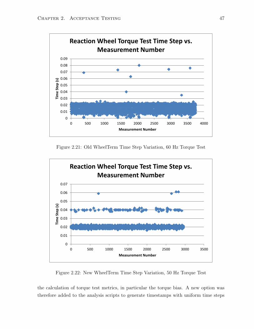
Chapter 2. Acceptance Testing 47
0
0.01
0.02
0.03
0.04
0.05
0.06
0.07
0.08
0.09
0 500 1000 1500 2000 2500 3000 3500 4000
Tim
e S
tep
(s)
Measurement Number
Reaction Wheel Torque Test Time Step vs. Measurement Number
Figure 2.21: Old WheelTerm Time Step Variation, 60 Hz Torque Test
0
0.01
0.02
0.03
0.04
0.05
0.06
0.07
0 500 1000 1500 2000 2500 3000 3500
Tim
e S
tep
(s)
Measurement Number
Reaction Wheel Torque Test Time Step vs. Measurement Number
Figure 2.22: New WheelTerm Time Step Variation, 50 Hz Torque Test
the calculation of torque test metrics, in particular the torque bias. A new option was
therefore added to the analysis scripts to generate timestamps with uniform time steps

Chapter 2. Acceptance Testing 48
between them the entire duration of the test divided by the number of data points.
This change helped reveal a previously unknown phenomenon – that the torque bias
is proportional to the applied torque. Specifically, the torque bias has been observed
to consistently equal approximately 0.55% of the applied torque. This behavior will be
captured in future iterations of Mirage, the attitude simulator, to determine its impact on
pointing performance, though the impact is expected to be small if it is at all noticeable.

Chapter 3
Conclusion
This thesis has contributed acceptance testing of attitude determination and control
system (ADCS) hardware for the AISSat-3, EV9, GHGSat-D, and NORSAT-1 missions
being developed by the Space Flight Laboratory at the University of Toronto Institute
for Aerospace Studies (UTIAS-SFL), as well as improvements to these tests and related
development and analysis work. In particular, acceptance testing was performed for
magnetometers, angular rate sensors, sun sensors, reaction wheels, magnetorquers, and
the GHGSat-D star tracker, and key contributions were made to the acceptance testing
procedures of magnetometers, angular rate sensors, sun sensors, and reaction wheels.
Updates were made to the magnetometer functional test, including the elimination of
the permanent magnet from the polarity check and the addition of a rough bias check.
The former eliminated a source of risk for the missions on which the magnetometers will
fly by reducing the chance that the magnetometer would be damaged or permanently
magnetized during testing. The latter allows the magnetometer bias to be checked more
frequently throughout the acceptance testing campaign, which facilitates troubleshooting
of anomalies encountered during testing and reduces the risk of delays in the acceptance
testing campaign by detecting faulty sensors early in the test cycle. An outdoor ver-
ification of the magnetometer calibration was also added. This test verified that the
calibration error of the magnetometers for each of the missions discussed in this thesis
was well below the alloted error in their pointing budgets.
The rate sensor calibration procedure was simplified and expedited with a reduction in
the number of calibration orientations from 21 to 9. It was found that this reduced num-
ber of orientations provides a comparable level of accuracy to the original 21 orientations
in determining the calibration parameters, and cuts the time required for calibrating the
rate sensor roughly in half. Additionally, a correlation was discovered between the screw
torque in the rate sensor daughter boards and the bias on the X- and Y-axis sensors,
49

Chapter 3. Conclusion 50
which reside on the daughter boards. The cause of this was determined to be stress ap-
plied by the screws to the sensor packages, affecting their measurement of Coriolis force.
It was determined that this issue was of minimum risk to the missions on which the rate
sensors will be flying, and that it would be impractical to design a replacement for the
upcoming missions. Recommendations for addressing this problem in future revisions of
the UTIAS-SFL rate sensor were to either increase the size of the daughter boards, or to
use adhesives to bond the daughter boards to their enclosures.
Corrections were made to the fine sun sensor calibration procedure in order to improve
the accuracy of the calibration. This included adding a sun source misalignment angle and
the vector between the sensor and rotator center of rotation to the calibration variables
estimated by the post-processing script. However, it was found that this extra freedom
was being exploited by the script to incorrectly compensate for unmodeled effects at the
edge of the sun sensor field of view, and was therefore producing unrealistic, unusable
results. Future work would test the calibration on only measurements collected within
a subset of the field of view in order to avoid including regions where the calibration
model breaks down, and explore the possibility of measuring and hardcoding the offset
between the sensor and rotator center of rotation. The results of these approaches would
be validated against on-orbit calibration results, and is expected to help eliminate a 2◦
calibration error observed in on-orbit operation of the sun sensors.
Finally, many improvements were contributed to the torque test in the reaction wheel
long-form functional test (LFFT). These included the replacement of the torque jitter
mean metric with the more meaningful angular velocity coefficient of determination, de-
veloping three new approaches to modeling the reaction wheel torque jitter as a simulated
noise source, adding an estimate of the area under the torque jitter fast Fourier transform
(FFT) magnitude plot as a new metric, and improving the uniformity of timestamps in
the data collected for the test. Examining the angular velocity coefficient of determi-
nation in the reaction wheel torque test helps to detect long-term deviations in applied
torque when the wheel is commanded to apply a constant torque, the occurrence of
which would indicate a faulty wheel or an error in the test setup. The three methods of
modeling torque jitter represent more rigorous approaches to simulating reaction wheel
performance in Mirage, UTIAS-SFL’s in-house attitude simulator, than what was previ-
ously implemented, providing better confidence in the representativeness of the models
to the wheels’ actual performance. The FFT area metric would help detect low-frequency
torque jitter anomalies, which could have an impact on satellite pointing performance,
though it was shown that the particular anomalies detected for the wheels tested in this
thesis did not. Finally, improving the uniformity of the test data timestamps has helped

Chapter 3. Conclusion 51
to improve the accuracy of the analysis performed on the data. Future work would im-
plement the three approaches to modeling torque jitter in Mirage and validating each
against on-orbit results in order to determine which approach provides the most accurate
simulation. Assessment of the effectiveness of the FFT magnitude plot area metric is
also pending.
The contributions of this thesis will contribute in large part to ensuring that the
hardware tested in this thesis and in the future will function and perform as demanded
by the mission and system requirements of the missions on which they will be flying, and
that the test procedures used to test the hardware are efficient and thorough.

Bibliography
[1] C. Grant et al., “On-orbit performance of the BRITE nanosatellite astronomy con-
stellation,” in 65th International Astronautical Congress, Toronto, Canada, 2014,
IAC-14-B4.2.3.
[2] J. R. Wertz, D. F. Everett, and J. J. Puschell, Space Mission Engineering: The New
SMAD. Microcosm Press, 2011, ch. 2.1, p. 37.
[3] W. J. Larson and J. R. Wertz, Space Mission Analysis and Design, 3rd ed. Micro-
cosm Press, 1999, ch. 12.1, p. 520.
[4] A. Philip, S. Eagleson et al., Test Plan, Procedure, and Results Report on Wheels
(Template), UTIAS-SFL, May 2015, SFL-AIM-ACS-TP002-2.1.
[5] G.-Y. Chung and R. E. Zee, Thermal Shock Test Procedure, UTIAS-SFL, August
2009, TPP0002A-1.3.
[6] R. E. Zee, UTIAS/SFL Thermal Vacuum and Standard Thermal Test Procedure,
UTIAS-SFL, TPP0001B-1.2.
[7] K. Sarda, “ADCS Hardware Temperature Limits,” UTIAS-SFL, Tech. Rep. SFL-
GEN-ACS-SP003-1.0, November 2014.
[8] “Nanosatellites: EV9,” University of Toronto Institute for Aerospace Studies Space
Flight Laboratory. [Online]. Available: http://utias-sfl.net/?page id=1271
[9] Nanosatellites: AISSat-3. University of Toronto Institute for Aerospace Studies
Space Flight Laboratory. [Online]. Available: http://utias-sfl.net/?page id=1268
[10] Microsatellites: GHGSat-D. University of Toronto Institute for Aerospace Studies
Space Flight Laboratory. [Online]. Available: http://utias-sfl.net/?page id=1254
[11] Microsatellites: NORSAT-1. University of Toronto Institute for Aerospace Studies
Space Flight Laboratory. [Online]. Available: http://utias-sfl.net/?page id=1260
52

Bibliography 53
[12] N. Ibrahim, “NEMO-AM attitude determination and control system design and
analysis,” UTIAS-SFL, Tech. Rep. SFL-NAM-ACS-D001-2.1, December 2014.
[13] S. Eagleson, “AISSat-1 attitude determination and control design document,”
UTIAS-SFL, Tech. Rep. SFL-AIS-ACS-D001-1.1, April 2008.
[14] S. Eagleson, K. Sarda, and Y. Shen, Test Plan, Procedures, and Results Report on
Magnetometers, UTIAS-SFL, August 2014, SFL-GNB-ACS-TP004-3.0.
[15] S. Eagleson and K. Sarda, Test Plan, Procedures, and Results Report on Magne-
tometers, UTIAS-SFL, February 2011, SFL-GNB-ACS-TP004-2.5.
[16] Operation Manual for Mag-03 Three-Axis Magnetic Field Sensors, Bartington In-
struments, Ltd., Witney, Oxford, UK, OM1004.
[17] Magnetic field calculators. NOAA National Centers for Environmental Information.
[Online]. Available: http://www.ngdc.noaa.gov/geomag-web/#igrfwmm
[18] R. Curey et al., IEEE Standard Specification Format Guide and Test Procedure for
Coriolis Vibratory Gyros, IEEE Aerospace and Electronic Systems Society, New
York, December 2004, IEEE-Std-1431-2004(R2010).
[19] S. Eagleson, K. Sarda et al., “Attitude determination and control CanX-4/5 sub-
system critical design review document,” UTIAS-SFL, Tech. Rep. SFL-CX4-CDR-
D003-1.0, March 2007.
[20] N. Roth, GNB Rate Sensor Calibration Procedure, UTIAS-SFL, January 2014, SFL-
GNB-ACS-TP012.
[21] 1270VS Single-Axis Rate Table Datasheet, Ideal Aerosmith, Inc., East Grand Forks,
MN, USA.
[22] M. Fournier, S. Eagleson, K. Sarda et al., Test Plan, Procedure and Results Report
on Rate Sensors, UTIAS-SFL, July 2015, SFL-GNB-ACS-TP006-2.3.
[23] E.-H. Shin and N. El-Sheimy, “A new calibration method for strapdown inertial
navigation systems,” Zeitschrift fur Vermessengswesen Journal, vol. 127, no. 1, pp.
1–10, 2001.
[24] S. Eagleson, K. Sarda, Y. Shen et al., Test Plan, Procedure and Results Report on
Sun Sensors, UTIAS-SFL, August 2014, SFL-GNB-ACS-TP010-2.8.

Bibliography 54
[25] P. Gavigan, “Design, test, calibration and qualification of satellite sun sensors,
power systems and supporting software development,” Master’s thesis, University of
Toronto, 2011.
[26] P. C. Hughes, Spacecraft Attitude Dynamics. Dover, 2004, ch. 6, p. 158.
[27] P. G. Lukaszynski, “Attitude control hardware and software for nanosatellites,”
Master’s thesis, University of Toronto, 2013.