Attacks Which Do Not Kill Training Make Adversarial ...
27
Attacks Which Do Not Kill Training Make Adversarial Learning Stronger Jingfeng Zhang * † 1 Xilie Xu *2 Bo Han 34 Gang Niu 4 Lizhen Cui 5 Masashi Sugiyama 46 Mohan Kankanhalli 1 Abstract Adversarial training based on the minimax for- mulation is necessary for obtaining adversarial robustness of trained models. However, it is con- servative or even pessimistic so that it sometimes hurts the natural generalization. In this paper, we raise a fundamental question—do we have to trade off natural generalization for adversarial ro- bustness? We argue that adversarial training is to employ confident adversarial data for updating the current model. We propose a novel formula- tion of friendly adversarial training (FAT): rather than employing most adversarial data maximiz- ing the loss, we search for least adversarial data (i.e., friendly adversarial data) minimizing the loss, among the adversarial data that are confi- dently misclassified. Our novel formulation is easy to implement by just stopping the most ad- versarial data searching algorithms such as PGD (projected gradient descent) early, which we call early-stopped PGD. Theoretically, FAT is justi- fied by an upper bound of the adversarial risk. Empirically, early-stopped PGD allows us to an- swer the earlier question negatively—adversarial robustness can indeed be achieved without com- promising the natural generalization. 1. Introduction Safety-critical nature of some areas such as medicine (Buch et al., 2018) and automatic driving (Litman, 2017), neces- * Equal contribution † Preliminary work was done during an internship at RIKEN AIP. 1 School of Computing, National Uni- versity of Singapore, Singapore 2 Taishan College, Shandong Uni- versity, Jinan, China 3 Department of Computer Science, Hong Kong Baptist University, Hong Kong, China 4 RIKEN Center for Advanced Intelligence Project (AIP), Tokyo, Japan 5 School of Soft- ware & Joint SDU-NTU Centre for Artificial Intelligence Research (C-FAIR), Shandong University, Jinan, China 6 Graduate School of Frontier Sciences, The University of Tokyo, Tokyo, Japan. Corre- spondence to: Jingfeng Zhang <[email protected]>. Proceedings of the 37 th International Conference on Machine Learning, Online, PMLR 119, 2020. Copyright 2020 by the au- thor(s). sitates the need for deep neural networks (DNNs) to be adversarially robust that generalize well. Recent research focuses on improving their robustness mainly by two de- fense approaches, i.e., certified defense and empirical de- fense. Certified defense tries to learn provably robust DNNs against norm-bounded (e.g., ‘ 2 and ‘ ∞ ) perturbations (Co- hen et al., 2019; Wong & Kolter, 2018; Tsuzuku et al., 2018; L´ ecuyer et al., 2019; Weng et al., 2018; Balunovic & Vechev, 2020; Zhang et al., 2020). Empirical defense incorporates adversarial data into the training process (Goodfellow et al., 2015; Madry et al., 2018; Cai et al., 2018; Zhang et al., 2019b; Wang et al., 2019; 2020). For instance, empirical defense has been used to train Wide ResNet (Zagoruyko & Komodakis, 2016) with natural data and its adversarial variants to make the trained network robust against strong adaptive attacks (Athalye et al., 2018; Carlini & Wagner, 2017). This paper belongs to the empirical defense category. Existing empirical defense methods formulate the adver- sarial training as a minimax optimization problem (Sec- tion 2.1)(Madry et al., 2018). To conduct this minimax op- timization, projected gradient descent (PGD) is a common method to generate the most adversarial data that maximizes the loss, updating the current model. PGD perturbs the nat- ural data for a fixed number of steps with small step size. After each step of perturbation, PGD projects the adversarial data back onto the -norm ball of the natural data. However, this minimax formulation is conservative (or even pessimistic), such that it sometimes hurts the natural gener- alization (Tsipras et al., 2019). For example, the top panels in Figure 1 show that at step #6 to #10 in PGD, the ad- versarial variants of the natural data significantly cross over the decision boundary and are located at their peer’s (natu- ral data) area. Since adversarial training aims to fit natural data and its adversarial variants simultaneously, such the cross-over mixture makes adversarial training extremely dif- ficult. Therefore, the most adversarial data generated by the PGD-10 (i.e., step #10 in top panel of Figure 1) directly “kill” the training, thus rendering the training unsuccessful. Inspired by philosopher Friedrich Nietzsche’s quote “that which does not kill us makes us stronger,” we propose friendly adversarial training (FAT): rather than employing the most adversarial data for updating the current model, we arXiv:2002.11242v2 [cs.LG] 5 Sep 2020
Transcript of Attacks Which Do Not Kill Training Make Adversarial ...
Attacks Which Do Not Kill Training Make Adversarial Learning Stronger
Jingfeng Zhang * † 1 Xilie Xu * 2 Bo Han 3 4 Gang Niu 4 Lizhen Cui 5
Masashi Sugiyama 4 6 Mohan Kankanhalli 1
AbstractAdversarial training based on the minimax for-mulation is necessary for obtaining adversarialrobustness of trained models. However, it is con-servative or even pessimistic so that it sometimeshurts the natural generalization. In this paper,we raise a fundamental question—do we have totrade off natural generalization for adversarial ro-bustness? We argue that adversarial training isto employ confident adversarial data for updatingthe current model. We propose a novel formula-tion of friendly adversarial training (FAT): ratherthan employing most adversarial data maximiz-ing the loss, we search for least adversarial data(i.e., friendly adversarial data) minimizing theloss, among the adversarial data that are confi-dently misclassified. Our novel formulation iseasy to implement by just stopping the most ad-versarial data searching algorithms such as PGD(projected gradient descent) early, which we callearly-stopped PGD. Theoretically, FAT is justi-fied by an upper bound of the adversarial risk.Empirically, early-stopped PGD allows us to an-swer the earlier question negatively—adversarialrobustness can indeed be achieved without com-promising the natural generalization.
1. IntroductionSafety-critical nature of some areas such as medicine (Buchet al., 2018) and automatic driving (Litman, 2017), neces-
*Equal contribution †Preliminary work was done during aninternship at RIKEN AIP. 1School of Computing, National Uni-versity of Singapore, Singapore 2Taishan College, Shandong Uni-versity, Jinan, China 3Department of Computer Science, HongKong Baptist University, Hong Kong, China 4RIKEN Center forAdvanced Intelligence Project (AIP), Tokyo, Japan 5School of Soft-ware & Joint SDU-NTU Centre for Artificial Intelligence Research(C-FAIR), Shandong University, Jinan, China 6Graduate School ofFrontier Sciences, The University of Tokyo, Tokyo, Japan. Corre-spondence to: Jingfeng Zhang <[email protected]>.
Proceedings of the 37 th International Conference on MachineLearning, Online, PMLR 119, 2020. Copyright 2020 by the au-thor(s).
sitates the need for deep neural networks (DNNs) to beadversarially robust that generalize well. Recent researchfocuses on improving their robustness mainly by two de-fense approaches, i.e., certified defense and empirical de-fense. Certified defense tries to learn provably robust DNNsagainst norm-bounded (e.g., `2 and `∞) perturbations (Co-hen et al., 2019; Wong & Kolter, 2018; Tsuzuku et al., 2018;Lecuyer et al., 2019; Weng et al., 2018; Balunovic & Vechev,2020; Zhang et al., 2020). Empirical defense incorporatesadversarial data into the training process (Goodfellow et al.,2015; Madry et al., 2018; Cai et al., 2018; Zhang et al.,2019b; Wang et al., 2019; 2020). For instance, empiricaldefense has been used to train Wide ResNet (Zagoruyko& Komodakis, 2016) with natural data and its adversarialvariants to make the trained network robust against strongadaptive attacks (Athalye et al., 2018; Carlini & Wagner,2017). This paper belongs to the empirical defense category.
Existing empirical defense methods formulate the adver-sarial training as a minimax optimization problem (Sec-tion 2.1) (Madry et al., 2018). To conduct this minimax op-timization, projected gradient descent (PGD) is a commonmethod to generate the most adversarial data that maximizesthe loss, updating the current model. PGD perturbs the nat-ural data for a fixed number of steps with small step size.After each step of perturbation, PGD projects the adversarialdata back onto the ε-norm ball of the natural data.
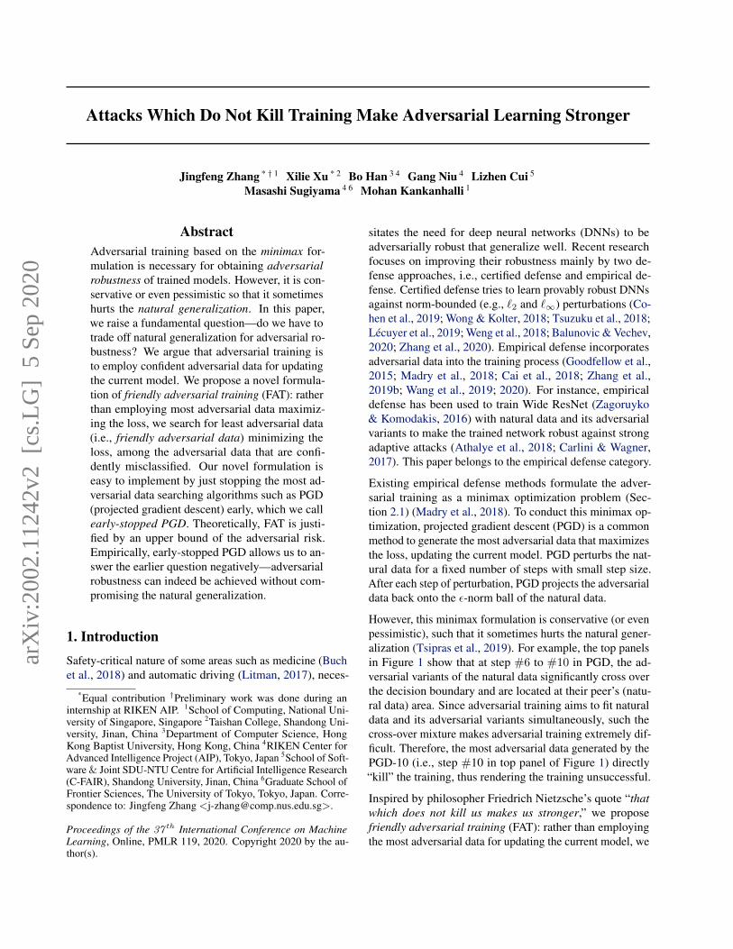
However, this minimax formulation is conservative (or evenpessimistic), such that it sometimes hurts the natural gener-alization (Tsipras et al., 2019). For example, the top panelsin Figure 1 show that at step #6 to #10 in PGD, the ad-versarial variants of the natural data significantly cross overthe decision boundary and are located at their peer’s (natu-ral data) area. Since adversarial training aims to fit naturaldata and its adversarial variants simultaneously, such thecross-over mixture makes adversarial training extremely dif-ficult. Therefore, the most adversarial data generated by thePGD-10 (i.e., step #10 in top panel of Figure 1) directly“kill” the training, thus rendering the training unsuccessful.
Inspired by philosopher Friedrich Nietzsche’s quote “thatwhich does not kill us makes us stronger,” we proposefriendly adversarial training (FAT): rather than employingthe most adversarial data for updating the current model, we
arX
iv:2
002.
1124
2v2
[cs
.LG
] 5
Sep
202
0
Friendly Adversarial Training
Natural data Step #1 Step #3 Step #6 Step #8 Step #10
Natural data Step #1 Step #3 Step #6 Step #8 Step #10
Figure 1. Green circles and yellow triangles are natural data forbinary classification. Red circles and blue triangles are adversarialvariants of green circles and yellow triangles, respectively. Blacksolid line is the decision boundary representing the current clas-sifier. Top: the adversarial data generated by PGD. Bottom: theadversarial data generated by early-stopped PGD.
search for the friendly adversarial data minimizing the loss.The friendly adversarial data are confidently misclassifiedby the current model. We design the learning objective ofFAT and theoretically justify it by deriving an upper boundof the adversarial risk (Section 3). Essentially, FAT updatesthe current model using friendly adversarial data. FAT trainsa DNN using the wrongly-predicted adversarial data mini-mizing the loss and the correctly-predicted adversarial datamaximizing the loss.
FAT is a reasonable strategy due to two reasons: It removesthe existing inconsistency between attack and defense, andit adheres to the spirit of curriculum learning. First, theways of generating adversarial data by adversarial attackersand adversarial defense methods are inconsistent. Adversar-ial attacks (Szegedy et al., 2014; Carlini & Wagner, 2017;Athalye et al., 2018) aim to find the adversarial data (notmaximizing the loss) to confidently fool the model. On theother hand, existing adversarial defense methods generatethe most adversarial data maximizing the loss regardless ofthe model’s predictions. These two should be harmonized.Second, the curriculum learning strategy has been shown tobe effective (Bengio et al., 2009). Fitting most adversarialdata initially makes the learning extremely difficult, some-times even killing the training. Instead, FAT learns initiallyfrom the least adversarial data and progressively utilizesincreasingly adversarial data.
FAT is easy to implement by just early stopping most-adversarial-data searching algorithms such as PGD, whichwe call early-stopped PGD (Section 4.1). Once adversar-ial data is misclassified by the current model, we stop thePGD iterations early. Early-stopped PGD has the benefit ofalleviating the cross-over mixture problem. For example,as shown in the bottom panels of Figure 1, adversarial datagenerated by early-stopped PGD will not be located at theirpeer areas (extensive details in Section 4.2). Thus, it will nothurt the generalization ability much. In addition, FAT basedon early-stopped PGD progressively employs stronger andstronger adversarial data (with more PGD steps), engender-ing increasingly enhanced robustness of the model over the
training progression (Section 5.3). This implies that attacksthat do not kill the training indeed make the adversariallearning stronger.
A brief overview of our contributions is as follows. Wepropose a novel formulation for adversarial learning (Sec-tion 3.1) and theoretically justify it by an upper bound ofthe adversarial risk (Section 3.2). Our FAT approximatelyrealizes this formulation by just stopping PGD early. FAThas the following benefits.
• Conventional adversarial training methods, e.g.,standard adversarial training (Madry et al., 2018),TRADES (Zhang et al., 2019b) and MART (Wanget al., 2020), can be easily modified to become friendlyadversarial training counterparts, i.e., FAT, FAT forTRADES, and FAT for MART (Section 5).
• Compared with conventional adversarial training, FAThas a better standard accuracy for natural data, whilekeeping a competitively robust accuracy for adversarialdata (Sections 5.1 and 6.2).
• FAT is computationally efficient because the earlystopped PGD saves a large number of backward propa-gations for searching adversarial data (Section 5.2).
• FAT can enable larger values of the perturbation bound,i.e., εtrain (Section 6.1), due to that FAT can alleviatethe cross-over mixture problem (Section 4.2).
With these benefits, FAT allows us to answer that adversarialrobustness can indeed be achieved without compromisingthe natural generalization.
2. Standard Adversarial TrainingLet (X , d∞) be the input feature space X with the infinitydistance metric dinf(x, x′) = ‖x− x′‖∞, and
Bε[x] = {x′ ∈ X | dinf(x, x′) ≤ ε} (1)
be the closed ball of radius ε > 0 centered at x in X .
2.1. Learning Objective
Given a dataset S = {(xi, yi)}ni=1, where xi ∈ X and yi ∈Y = {0, 1, ..., C − 1}, the objective function of standardadversarial training (Madry et al., 2018) is
minf∈F
1
n
n∑i=1
{max
x∈Bε[xi]`(f(x), yi)
}, (2)
where x is the adversarial data within the ε-ball centeredat x, f(·) : X → RC is a score function, and the lossfunction ` : RC × Y → R is a composition of a base loss
Friendly Adversarial Training
𝑋
𝑋′
𝑋′′
𝑋𝑋!! = 𝑋′
0/1 loss
Logistic loss
0
1
-1
0
1 0-1 1
1
0
𝜌 = {
𝑋!!: Most adversarial data
𝑋′: Fridendly adversarial data (ours)
𝑋: Natural data
When adversarial data are wrongly predicted When adversarial data are correctly predicted
Figure 2. In adversarial training, the adversarial data is generated within the perturbation ball Bε[X] of natural data X given the currentmodel f . The existing adversarial training generates most adversarial data X
′′that maximizes the inner loss regardless of their predictions.
FAT takes their predictions into account. When the model makes the wrong predictions of adversarial data, our friendly adversarial dataX ′ minimizes the inner loss by a violation of a small constant ρ.
`B : ∆C−1 × Y → R (e.g., the cross-entropy loss) and aninverse link function `L : RC → ∆C−1 (e.g., the soft-maxactivation), in which ∆C−1 is the corresponding probabilitysimplex—in other words, `(f(·), y) = `B(`L(f(·)), y).
For the sake of conceptual consistency, the objective func-tion (i.e., Eq. (2)) can also be re-written as
minf∈F
1
n
n∑i=1
`(f(xi), yi), (3)
where
xi = arg maxx∈Bε[xi] `(f(x), yi). (4)
It implies the optimization of adversariallly robust network,with one step maximizing loss to find adversarial data andone step minimizing loss on the adversarial data w.r.t. thenetwork parameters θ.
2.2. Projected Gradient Descent (PGD)
To generate adversarial data, standard adversarial traininguses PGD to approximately solve the inner maximization ofEq. (4) (Madry et al., 2018).
PGD formulates the problem of finding adversarial data as aconstrained optimization problem. Namely, given a startingpoint x(0) ∈ X and step size α > 0, PGD works as follows:
x(t+1) = ΠB[x(0)]
(x(t)+α sign(∇x(t)`(fθ(x
(t)), y))),∀t ≥ 0
(5)
until a certain stopping criterion is satisfied. For example,the criterion can be a fixed number of iterations K, namelythe PGD-K algorithm (Madry et al., 2018; Wang et al.,2020). In Eq. (5), ` is the loss function in Eq. (4); x(0) refersto natural data or natural data corrupted by a small Gaussianor uniform random noise; y is the corresponding label fornatural data; x(t) is adversarial data at step t; and ΠBε[x0](·)is the projection function that projects the adversarial databack into the ε-ball centered at x(0) if necessary.
There are also other ways to generate adversarial data, e.g.,the fast gradient signed method (Szegedy et al., 2014; Good-fellow et al., 2015), the CW attack (Carlini & Wagner, 2017),deformation attack (Alaifari et al., 2019; Xiao et al., 2018),and Hamming distance method (Shamir et al., 2019).
PGD adversarial training. Besides the standard adver-sarial training, several improvements to PGD adversarialtraining have also been proposed, such as Lipschitz regular-ization (Cisse et al., 2017; Hein & Andriushchenko, 2017;Yan et al., 2018; Farnia et al., 2019), curriculum adversarialtraining (Cai et al., 2018; Wang et al., 2019), computa-tionally efficient adversarial learning (Shafahi et al., 2019;Zhang et al., 2019a; Wong et al., 2020), ensemble adversar-ial training (Tramr et al., 2018; Pang et al., 2019), and ad-versarial training by utilizing unlabeled data (Carmon et al.,2019; Najafi et al., 2019; Alayrac et al., 2019). In addition,TRADES (Zhang et al., 2019b) and MART (Wang et al.,2020) are effective adversarial training methods, whichtrains on both natural data x and adversarial data x (the learn-
Friendly Adversarial Training
ing objectives are reviewed in Appendices D.1 and E.1 re-spectively). Moreover, there are interesting analyses of PGDadversarial training, such as showing overfitting in PGD-adversarial training (Rice et al., 2020), disentangling robustand non-robust features through PGD-adversarially trainednetwork (Ilyas et al., 2019), showing different feature repre-sentations by robust model and non-robust model (Tsipraset al., 2019), and providing a new explanation for the trade-off between robustness and accuracy of PGD-adversarialtraining (Raghunathan et al., 2020).
3. Friendly Adversarial TrainingIn this section, we develop a novel learning objective forfriendly adversarial training (FAT). Theoretically, we justifyFAT by deriving a tight upper bound of the adversarial risk.
3.1. Learning Objective
Let ρ > 0 be a margin such that our adversarial data wouldbe misclassified with a certain amount of confidence.
The outer minimization still follows Eq. (3). However, in-stead of generating xi via inner maximization, we generatexi as follows:
xi = arg minx∈Bε[xi]
`(f(x), yi)
s.t. `(f(x), yi)−miny∈Y `(f(x), y) ≥ ρ.
Note that the operator arg max in Eq. (4) is replaced witharg min here, and there is a constraint on the margin of lossvalues (i.e., the misclassification confidence).
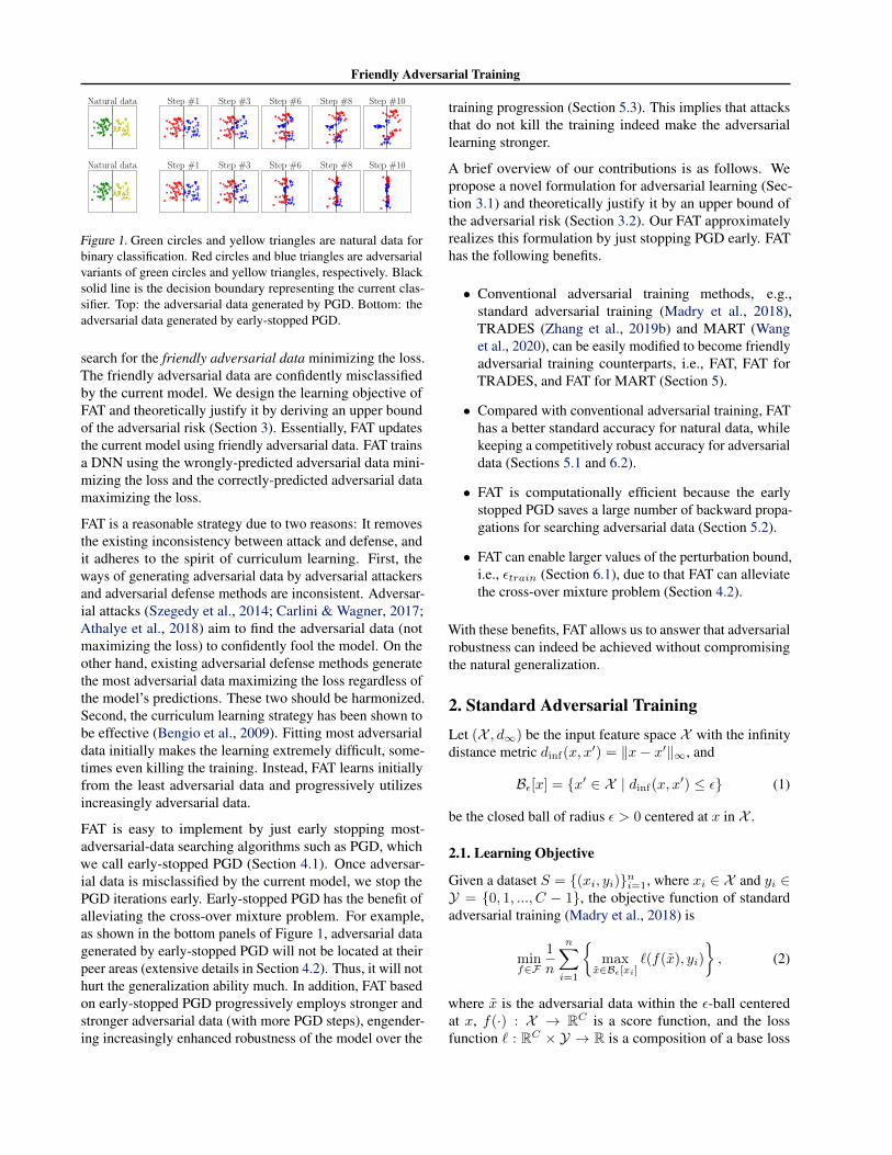
The constraint firstly ensures yi 6= arg miny∈Y `(f(x), y)or x is misclassified, and secondly ensures for x the wrongprediction is better than the desired prediction yi by at leastρ in terms of the loss value. Among all such x satisfyingthe constraint, we select the one minimizing `(f(x), yi).Namely, we minimize the adversarial loss given that someconfident adversarial data has been found. This xi couldbe regarded as a “friend” among the adversaries, which istermed friendly adversarial data. Figure 2 illustrates thedifferences between our learning objective and the conven-tional minimax formulation.
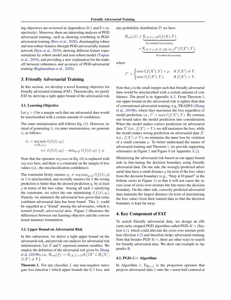
3.2. Upper Bound on Adversarial Risk
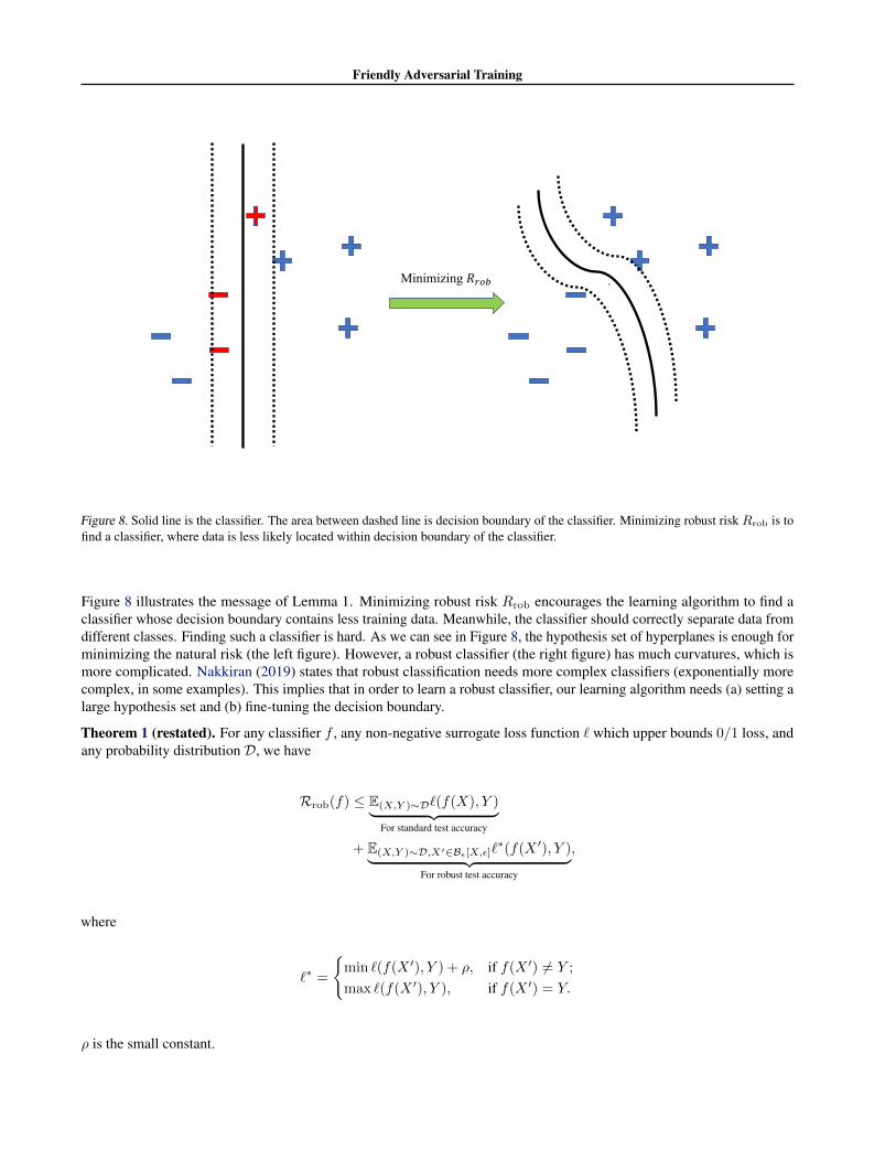
In this subsection, we derive a tight upper bound on theadversarial risk, and provide our analysis for adversarial riskminimization. Let X and Y represent random variables. Weemploy the definition of the adversarial risk given by Zhanget al. (2019b), i.e.,Rrob(f) := E(X,Y )∼D1{∃X ′ ∈ Bε[X] :f(X ′) 6= Y }.Theorem 1. For any classifier f , any non-negative surro-gate loss function ` which upper bounds the 0/1 loss, and
any probability distribution D, we have
Rrob(f) ≤ E(X,Y )∼D`(f(X), Y )︸ ︷︷ ︸For standard test accuracy
+ E(X,Y )∼D,X′∈Bε[X,ε]`∗(f(X ′), Y )︸ ︷︷ ︸
For robust test accuracy
,
where
`∗ =
{min `(f(X ′), Y ) + ρ, if f(X ′) 6= Y,
max `(f(X ′), Y ), if f(X ′) = Y.
Note that ρ is the small margin such that friendly adversarialdata would be misclassified with a certain amount of con-fidence. The proof is in Appendix A.2. From Theorem 1,our upper bound on the adversarial risk is tighter than thatof conventional adversarial training, e.g.,TRADES (Zhanget al., 2019b), where they maximize the loss regardless ofmodel prediction, i.e., `∗ = max `(f(X ′), Y ). By contrast,our bound takes the model prediction into consideration.When the model makes correct prediction on adversarialdataX ′ (i.e., f(X ′) = Y ), we still maximize the loss; whilethe model makes wrong prediction on adversarial data X ′
(i.e., f(X ′) 6= Y ), we minimize the inner loss by violationof a small constant ρ. To better understand the nature ofadversarial training and Theorem 1, we provide supportingschematics in Figure 2 and Figure 8 (in Appendix A.2).
Minimizing the adversarial risk based on our upper boundaids in fine-tuning the decision boundary using friendlyadversarial data. On one side, the wrongly-predicted adver-sarial data have a small distance ρ (in term of the loss value)from the decision boundary (e.g., “Step #10 panel” at thebottom series in Figure 1) so that it will not cause the se-vere issue of cross-over mixture but fine-tunes the decisionboundary. On the other side, correctly-predicted adversarialdata maintain the largest distance (in term of maximizingthe loss value) from their natural data so that the decisionboundary is kept far away.
4. Key Component of FATTo search friendly adversarial data, we design an effi-cient early-stopped PGD algorithm called PGD-K-τ (Sec-tion 4.1), which could alleviate the cross-over mixture prob-lem (Section 4.2) and therefore helps adversarial training.Note that besides PGD-K-τ , there are other ways to searchfor friendly adversarial data. We show one example in Ap-pendix B.
4.1. PGD-K-τ Algorithm
In Algorithm 1, ΠB[x,ε] is the projection operator thatprojects adversarial data x onto the ε-norm ball centered at
Friendly Adversarial Training
Algorithm 1 PGD-K-τInput: data x ∈ X , label y ∈ Y , model f , loss function`, maximum PGD step K, step τ , perturbation bound ε,step size αOutput: xx← xwhile K > 0 do
if arg maxi f(x) 6= y and τ = 0 thenbreak
else if arg maxi f(x) 6= y thenτ ← τ − 1
end ifx← ΠB[x,ε]
(α sign(∇x`(f(x), y)) + x
)K ← K − 1
end while
x, and arg maxi f(x) returns the predicted label of adver-sarial data x, where f(x) =
(f i(x)
)>i=0,...,C−1 measures
the probabilistic predictions over C classes. Unlike theconventional PGD-K generating adversarial data by max-imizing the loss function ` regardless of model prediction,our PGD-K-τ generates the adversarial data which takesmodel prediction into consideration.
Algorithm 1 returns the misclassified adversarial data withsmall loss values or correctly classified adversarial datawith large loss values. Step τ controls the extent of lossminimization when misclassified adversarial data are found.When τ is larger, the misclassified adversarial data withslightly larger loss values are returned, and vice versa. τ×αis an approximation to ρ in our learning objective. Note thatwhen τ = K, the conventional PGD-K is the special caseof our PGD-K-τ . As τ is an important hyper-parameter ofPGD-K-τ for FAT (Section 5), we discuss how to select τin Sections 5.1 and 5.2 in detail.
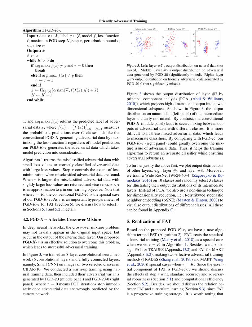
4.2. PGD-K-τ Alleviates Cross-over Mixture
In deep neural networks, the cross-over mixture problemmay not trivially appear in the original input space, butoccur in the output of the intermediate layer. Our proposedPGD-K-τ is an effective solution to overcome this problem,which leads to successful adversarial training.
In Figure 3, we trained an 8-layer convolutional neural net-work (6 convolutional layers and 2 fully-connected layers,namely, Small CNN) on images of two selected classes inCIFAR-10. We conducted a warm-up training using nat-ural training data, then included their adversarial variantsgenerated by PGD-20 (middle panel) and PGD-20-0 (rightpanel), where τ = 0 means PGD iterations stop immedi-ately once adversarial data are wrongly predicted by thecurrent network.
0 50
−20
0
20
Natural data (layer #7)
−100 0 100
−25
0
25
PGD-K (layer #7)
−100 0 100
−20
0
20
40
PGD-K-τ (layer #7)
Figure 3. Left: layer #7’s output distribution on natural data (notmixed). Middle: layer #7’s output distribution on adversarialdata generated by PGD-20 (significantly mixed). Right: layer#7’s output distribution on friendly adversarial data generated byPGD-20-0 (not significantly mixed).
Figure 3 shows the output distribution of layer #7 byprincipal component analysis (PCA, (Abdi & Williams,2010)), which projects high-dimensional output into a two-dimensional subspace. As shown in Figure 3, the outputdistribution on natural data (left panel) of the intermediatelayer is clearly not mixed. By contrast, the conventionalPGD-K (middle panel) leads to severe mixing between out-puts of adversarial data with different classes. It is moredifficult to fit these mixed adversarial data, which leadsto inaccurate classifiers. By comparing with PGD-K, ourPGD-K-τ (right panel) could greatly overcome the mix-ture issue of adversarial data. Thus, it helps the trainingalgorithm to return an accurate classifier while ensuringadversarial robustness.
To further justify the above fact, we plot output distributionsof other layers, e.g., layer #6 and layer #8. Moreover,we train a Wide ResNet (WRN-40-4) (Zagoruyko & Ko-modakis, 2016) on 10 classes and randomly select 3 classesfor illustrating their output distributions of its intermediatelayers. Instead of PCA, we also use a non-linear techniquefor dimensionality reduction, i.e., t-distributed stochasticneighbor embedding (t-SNE) (Maaten & Hinton, 2008) tovisualize output distributions of different classes. All thesecan be found in Appendix C.
5. Realization of FATBased on the proposed PGD-K-τ , we have a new algo-rithm termed FAT (Algorithm 2). FAT treats the standardadversarial training (Madry et al., 2018) as a special casewhen we set τ = K in Algorithm 1. Besides, we also de-sign FAT for TRADES (Appendix D.2) and FAT for MART(Appendix E.2), making two effective adversarial trainingmethods (TRADES (Zhang et al., 2019b) and MART (Wanget al., 2020)) special cases when τ = K. Since the essen-tial component of FAT is PGD-K-τ , we should discussthe effects of step τ w.r.t. standard accuracy and adversar-ial robustness (Section 5.1) and computational efficiency(Section 5.2). Besides, we should discuss the relation be-tween FAT and curriculum learning (Section 5.3), since FATis a progressive training strategy. It is worth noting that
Friendly Adversarial Training
Algorithm 2 Friendly Adversarial Training (FAT)Input: network fθ, training dataset S = {(xi, yi)}ni=1,learning rate η, number of epochs T , batch size m, num-ber of batches MOutput: adversarially robust network fθfor epoch = 1, . . . , T do
for mini-batch = 1, . . . , M doSample a mini-batch {(xi, yi)}mi=1 from Sfor i = 1, . . . , m (in parallel) do
Obtain adversarial data xiof xi by Algorithm 1end forθ ← θ − η 1
m
∑mi−1∇θ`(fθ(xi), yi)
end forend for
Sitawarin et al. (2020) independently propose adversarialtraining with early stopping (ATES). Along with our FAT,ATES corroborates the new formulation (Section 3.1) foradversarial training.
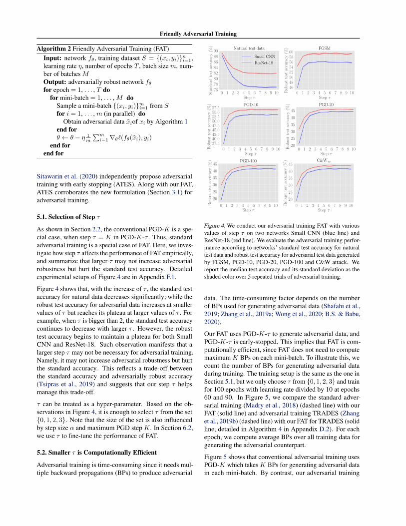
5.1. Selection of Step τ
As shown in Section 2.2, the conventional PGD-K is a spe-cial case, when step τ = K in PGD-K-τ . Thus, standardadversarial training is a special case of FAT. Here, we inves-tigate how step τ affects the performance of FAT empirically,and summarize that larger τ may not increase adversarialrobustness but hurt the standard test accuracy. Detailedexperimental setups of Figure 4 are in Appendix F.1.
Figure 4 shows that, with the increase of τ , the standard testaccuracy for natural data decreases significantly; while therobust test accuracy for adversarial data increases at smallervalues of τ but reaches its plateau at larger values of τ . Forexample, when τ is bigger than 2, the standard test accuracycontinues to decrease with larger τ . However, the robusttest accuracy begins to maintain a plateau for both SmallCNN and ResNet-18. Such observation manifests that alarger step τ may not be necessary for adversarial training.Namely, it may not increase adversarial robustness but hurtthe standard accuracy. This reflects a trade-off betweenthe standard accuracy and adversarially robust accuracy(Tsipras et al., 2019) and suggests that our step τ helpsmanage this trade-off.
τ can be treated as a hyper-parameter. Based on the ob-servations in Figure 4, it is enough to select τ from the set{0, 1, 2, 3}. Note that the size of the set is also influencedby step size α and maximum PGD step K. In Section 6.2,we use τ to fine-tune the performance of FAT.
5.2. Smaller τ is Computationally Efficient
Adversarial training is time-consuming since it needs mul-tiple backward propagations (BPs) to produce adversarial
0 1 2 3 4 5 6 7 8 9 10Step τ
7678808284868890
Sta
nd
ard
test
accu
racy
(%)
Natural test data
Small CNN
ResNet-18
0 1 2 3 4 5 6 7 8 9 10Step τ
4648505254565860
Rob
ust
test
accu
racy
(%) FGSM
0 1 2 3 4 5 6 7 8 9 10Step τ
37.540.042.545.047.550.052.555.057.5
Rob
ust
test
accu
racy
(%) PGD-10
0 1 2 3 4 5 6 7 8 9 10Step τ
20
25
30
35
40
45
Rob
ust
test
accu
racy
(%) PGD-20
0 1 2 3 4 5 6 7 8 9 10Step τ
20
25
30
35
40
45
Rob
ust
test
accu
racy
(%) PGD-100
0 1 2 3 4 5 6 7 8 9 10Step τ
20
25
30
35
40
45
Rob
ust
test
accu
racy
(%) C&W∞
Figure 4. We conduct our adversarial training FAT with variousvalues of step τ on two networks Small CNN (blue line) andResNet-18 (red line). We evaluate the adversarial training perfor-mance according to networks’ standard test accuracy for naturaltest data and robust test accuracy for adversarial test data generatedby FGSM, PGD-10, PGD-20, PGD-100 and C&W attack. Wereport the median test accuracy and its standard deviation as theshaded color over 5 repeated trials of adversarial training.
data. The time-consuming factor depends on the numberof BPs used for generating adversarial data (Shafahi et al.,2019; Zhang et al., 2019a; Wong et al., 2020; B.S. & Babu,2020).
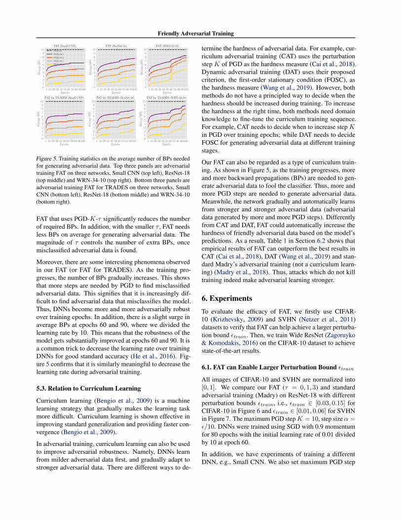
Our FAT uses PGD-K-τ to generate adversarial data, andPGD-K-τ is early-stopped. This implies that FAT is com-putationally efficient, since FAT does not need to computemaximum K BPs on each mini-batch. To illustrate this, wecount the number of BPs for generating adversarial dataduring training. The training setup is the same as the one inSection 5.1, but we only choose τ from {0, 1, 2, 3} and trainfor 100 epochs with learning rate divided by 10 at epochs60 and 90. In Figure 5, we compare the standard adver-sarial training (Madry et al., 2018) (dashed line) with ourFAT (solid line) and adversarial training TRADES (Zhanget al., 2019b) (dashed line) with our FAT for TRADES (solidline, detailed in Algorithm 4 in Appendix D.2). For eachepoch, we compute average BPs over all training data forgenerating the adversarial counterpart.
Figure 5 shows that conventional adversarial training usesPGD-K which takes K BPs for generating adversarial datain each mini-batch. By contrast, our adversarial training
Friendly Adversarial Training
1 10 20 30 40 50 60 70 80 90100Epochs
0
1
2
3
4
5
6
7
8
9
10
Ave
rage
BP
s
FAT (Small CNN)
PGD-10
PGD-10-3
PGD-10-2
PGD-10-1
PGD-10-0
1 10 20 30 40 50 60 70 80 90100Epochs
0123456789
10
Ave
rage
BP
s
FAT (ResNet-18)
1 10 20 30 40 50 60 70 80 90100Epochs
0123456789
10
Ave
rage
BP
s
FAT (WRN-34-10)
1 10 20 30 40 50 60 70 80 90100Epochs
0123456789
10
Ave
rage
BP
s
FAT for TRADES (Small CNN)
1 10 20 30 40 50 60 70 80 90100Epochs
0123456789
10
Ave
rage
BP
s
FAT for TRADES (ResNet-18)
1 10 20 30 40 50 60 70 80 90100Epochs
0123456789
10
Ave
rage
BP
s
FAT for TRADES (WRN-34-10)
Figure 5. Training statistics on the average number of BPs neededfor generating adversarial data. Top three panels are adversarialtraining FAT on three networks, Small CNN (top left), ResNet-18(top middle) and WRN-34-10 (top right). Bottom three panels areadversarial training FAT for TRADES on three networks, SmallCNN (bottom left), ResNet-18 (bottom middle) and WRN-34-10(bottom right).
FAT that uses PGD-K-τ significantly reduces the numberof required BPs. In addition, with the smaller τ , FAT needsless BPs on average for generating adversarial data. Themagnitude of τ controls the number of extra BPs, oncemisclassified adversarial data is found.
Moreover, there are some interesting phenomena observedin our FAT (or FAT for TRADES). As the training pro-gresses, the number of BPs gradually increases. This showsthat more steps are needed by PGD to find misclassifiedadversarial data. This signifies that it is increasingly dif-ficult to find adversarial data that misclassifies the model.Thus, DNNs become more and more adversarially robustover training epochs. In addition, there is a slight surge inaverage BPs at epochs 60 and 90, where we divided thelearning rate by 10. This means that the robustness of themodel gets substantially improved at epochs 60 and 90. It isa common trick to decrease the learning rate over trainingDNNs for good standard accuracy (He et al., 2016). Fig-ure 5 confirms that it is similarly meaningful to decrease thelearning rate during adversarial training.
5.3. Relation to Curriculum Learning
Curriculum learning (Bengio et al., 2009) is a machinelearning strategy that gradually makes the learning taskmore difficult. Curriculum learning is shown effective inimproving standard generalization and providing faster con-vergence (Bengio et al., 2009).
In adversarial training, curriculum learning can also be usedto improve adversarial robustness. Namely, DNNs learnfrom milder adversarial data first, and gradually adapt tostronger adversarial data. There are different ways to de-
termine the hardness of adversarial data. For example, cur-riculum adversarial training (CAT) uses the perturbationstep K of PGD as the hardness measure (Cai et al., 2018).Dynamic adversarial training (DAT) uses their proposedcriterion, the first-order stationary condition (FOSC), asthe hardness measure (Wang et al., 2019). However, bothmethods do not have a principled way to decide when thehardness should be increased during training. To increasethe hardness at the right time, both methods need domainknowledge to fine-tune the curriculum training sequence.For example, CAT needs to decide when to increase step Kin PGD over training epochs; while DAT needs to decideFOSC for generating adversarial data at different trainingstages.
Our FAT can also be regarded as a type of curriculum train-ing. As shown in Figure 5, as the training progresses, moreand more backward propagations (BPs) are needed to gen-erate adversarial data to fool the classifier. Thus, more andmore PGD steps are needed to generate adversarial data.Meanwhile, the network gradually and automatically learnsfrom stronger and stronger adversarial data (adversarialdata generated by more and more PGD steps). Differentlyfrom CAT and DAT, FAT could automatically increase thehardness of friendly adversarial data based on the model’spredictions. As a result, Table 1 in Section 6.2 shows thatempirical results of FAT can outperform the best results inCAT (Cai et al., 2018), DAT (Wang et al., 2019) and stan-dard Madry’s adversarial training (not a curriculum learn-ing) (Madry et al., 2018). Thus, attacks which do not killtraining indeed make adversarial learning stronger.
6. ExperimentsTo evaluate the efficacy of FAT, we firstly use CIFAR-10 (Krizhevsky, 2009) and SVHN (Netzer et al., 2011)datasets to verify that FAT can help achieve a larger perturba-tion bound εtrain. Then, we train Wide ResNet (Zagoruyko& Komodakis, 2016) on the CIFAR-10 dataset to achievestate-of-the-art results.
6.1. FAT can Enable Larger Perturbation Bound εtrain
All images of CIFAR-10 and SVHN are normalized into[0, 1]. We compare our FAT (τ = 0, 1, 3) and standardadversarial training (Madry) on ResNet-18 with differentperturbation bounds εtrain, i.e., εtrain ∈ [0.03, 0.15] forCIFAR-10 in Figure 6 and εtrain ∈ [0.01, 0.06] for SVHNin Figure 7. The maximum PGD stepK = 10, step size α =ε/10. DNNs were trained using SGD with 0.9 momentumfor 80 epochs with the initial learning rate of 0.01 dividedby 10 at epoch 60.
In addition, we have experiments of training a differentDNN, e.g., Small CNN. We also set maximum PGD step
Friendly Adversarial Training
0.03 0.06 0.09 0.12 0.15Perturbation bound εtrain
30
40
50
60
70
80
90S
tan
dar
dte
stac
cura
cy(%
)Natural test data
Madry
FAT (τ = 0)
FAT (τ = 1)
FAT (τ = 3)
0.03 0.06 0.09 0.12 0.15Perturbation bound εtrain
2530354045505560
Rob
ust
test
accu
racy
(%) FGSM
0.03 0.06 0.09 0.12 0.15Perturbation bound εtrain
25
30
35
40
45
50
Rob
ust
test
accu
racy
(%) PGD-20 (εtest = 8/255)
0.03 0.06 0.09 0.12 0.15Perturbation bound εtrain
25
30
35
40
45
Rob
ust
test
accu
racy
(%) C&W∞
0.03 0.06 0.09 0.12 0.15Perturbation bound εtrain
25
30
35
40
45
50
Rob
ust
test
accu
racy
(%) PGD-100
0.03 0.06 0.09 0.12 0.15Perturbation bound εtrain
10
15
20
25
30
35
Rob
ust
test
accu
racy
(%) PGD-20 (εtest = 16/255)
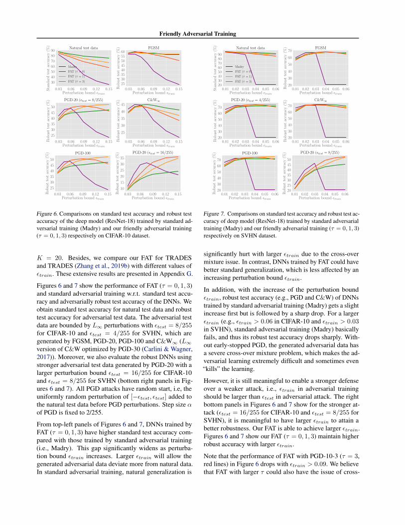
Figure 6. Comparisons on standard test accuracy and robust testaccuracy of the deep model (ResNet-18) trained by standard ad-versarial training (Madry) and our friendly adversarial training(τ = 0, 1, 3) respectively on CIFAR-10 dataset.
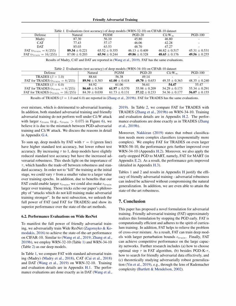
K = 20. Besides, we compare our FAT for TRADESand TRADES (Zhang et al., 2019b) with different values ofεtrain. These extensive results are presented in Appendix G.
Figures 6 and 7 show the performance of FAT (τ = 0, 1, 3)and standard adversarial training w.r.t. standard test accu-racy and adversarially robust test accuracy of the DNNs. Weobtain standard test accuracy for natural test data and robusttest accuracy for adversarial test data. The adversarial testdata are bounded by L∞ perturbations with εtest = 8/255for CIFAR-10 and εtest = 4/255 for SVHN, which aregenerated by FGSM, PGD-20, PGD-100 and C&W∞ (L∞version of C&W optimized by PGD-30 (Carlini & Wagner,2017)). Moreover, we also evaluate the robust DNNs usingstronger adversarial test data generated by PGD-20 with alarger perturbation bound εtest = 16/255 for CIFAR-10and εtest = 8/255 for SVHN (bottom right panels in Fig-ures 6 and 7). All PGD attacks have random start, i.e, theuniformly random perturbation of [−εtest, εtest] added tothe natural test data before PGD perturbations. Step size αof PGD is fixed to 2/255.
From top-left panels of Figures 6 and 7, DNNs trained byFAT (τ = 0, 1, 3) have higher standard test accuracy com-pared with those trained by standard adversarial training(i.e., Madry). This gap significantly widens as perturba-tion bound εtrain increases. Larger εtrain will allow thegenerated adversarial data deviate more from natural data.In standard adversarial training, natural generalization is
0.01 0.02 0.03 0.04 0.05 0.06Perturbation bound εtrain
2030405060708090
Sta
nd
ard
test
accu
racy
(%)
Natural test data
Madry
FAT (τ = 0)
FAT (τ = 1)
FAT (τ = 3)
0.01 0.02 0.03 0.04 0.05 0.06Perturbation bound εtrain
20
30
40
50
60
70
Rob
ust
test
accu
racy
(%) FGSM
0.01 0.02 0.03 0.04 0.05 0.06Perturbation bound εtrain
20
30
40
50
60
70
Rob
ust
test
accu
racy
(%) PGD-20 (εtest = 4/255)
0.01 0.02 0.03 0.04 0.05 0.06Perturbation bound εtrain
20
30
40
50
60
70
Rob
ust
test
accu
racy
(%) C&W∞
0.01 0.02 0.03 0.04 0.05 0.06Perturbation bound εtrain
20
30
40
50
60
70
Rob
ust
test
accu
racy
(%) PGD-100
0.01 0.02 0.03 0.04 0.05 0.06Perturbation bound εtrain
20253035404550
Rob
ust
test
accu
racy
(%) PGD-20 (εtest = 8/255)
Figure 7. Comparisons on standard test accuracy and robust test ac-curacy of deep model (ResNet-18) trained by standard adversarialtraining (Madry) and our friendly adversarial training (τ = 0, 1, 3)respectively on SVHN dataset.
significantly hurt with larger εtrain due to the cross-overmixture issue. In contrast, DNNs trained by FAT could havebetter standard generalization, which is less affected by anincreasing perturbation bound εtrain.
In addition, with the increase of the perturbation boundεtrain, robust test accuracy (e.g., PGD and C&W) of DNNstrained by standard adversarial training (Madry) gets a slightincrease first but is followed by a sharp drop. For a largerεtrain (e.g., εtrain > 0.06 in CIFAR-10 and εtrain > 0.03in SVHN), standard adversarial training (Madry) basicallyfails, and thus its robust test accuracy drops sharply. With-out early-stopped PGD, the generated adversarial data hasa severe cross-over mixture problem, which makes the ad-versarial learning extremely difficult and sometimes even“kills” the learning.
However, it is still meaningful to enable a stronger defenseover a weaker attack, i.e., εtrain in adversarial trainingshould be larger than εtest in adversarial attack. The rightbottom panels in Figures 6 and 7 show for the stronger at-tack (εtest = 16/255 for CIFAR-10 and εtest = 8/255 forSVHN), it is meaningful to have larger εtrain to attain abetter robustness. Our FAT is able to achieve larger εtrain.Figures 6 and 7 show our FAT (τ = 0, 1, 3) maintain higherrobust accuracy with larger εtrain.
Note that the performance of FAT with PGD-10-3 (τ = 3,red lines) in Figure 6 drops with εtrain > 0.09. We believethat FAT with larger τ could also have the issue of cross-
Friendly Adversarial Training
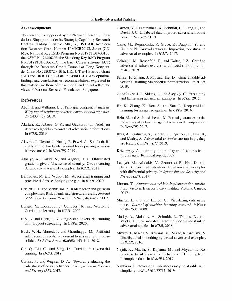
Table 1. Evaluations (test accuracy) of deep models (WRN-32-10) on CIFAR-10 datasetDefense Natural FGSM PGD-20 C&W∞ PGD-100Madry 87.30 56.10 45.80 46.80 -CAT 77.43 57.17 46.06 42.28 -DAT 85.03 63.53 48.70 47.27 -
FAT (εtrain = 8/255) 89.34 ± 0.221 65.52 ± 0.355 46.13 ± 0.409 46.82 ± 0.517 45.31 ± 0.531FAT (εtrain = 16/255) 87.00 ± 0.203 65.94 ± 0.244 49.86 ± 0.328 48.65 ± 0.176 49.56 ± 0.255
Results of Madry, CAT and DAT are reported in (Wang et al., 2019). FAT has the same evaluations.
Table 2. Evaluations (test accuracy) of deep models (WRN-34-10) on CIFAR-10 datasetDefense Natural FGSM PGD-20 C&W∞ PGD-100
TRADES (β = 1.0) 88.64 56.38 49.14 - -FAT for TRADES (εtrain = 8/255) 89.94 ± 0.303 61.00 ± 0.418 49.70 ± 0.653 49.35 ± 0.363 48.35 ± 0.240
TRADES (β = 6.0) 84.92 61.06 56.61 54.47 55.47FAT for TRADES (εtrain = 8/255) 86.60 ± 0.548 61.97 ± 0.570 55.98 ± 0.209 54.29 ± 0.173 55.34 ± 0.291
FAT for TRADES (εtrain = 16/255) 84.39 ± 0.030 61.73 ± 0.131 57.12 ± 0.233 54.36 ± 0.177 56.07 ± 0.155
Results of TRADES (β = 1.0 and 6.0) are reported in (Zhang et al., 2019b). FAT for TRADES has the same evaluations.
over mixture, which is detrimental to adversarial learning.In addition, both standard adversarial training and friendlyadversarial training do not perform well under C&W attackwith larger εtrain (e.g., εtrain > 0.075 in Figure 6), webelieve it is due to the mismatch between PGD-adversarialtraining and C&W attack. We discuss the reasons in detailin Appendix G.4.
To sum up, deep models by FAT with τ = 0 (green line)have higher standard test accuracy, but lower robust testaccuracy. By increasing τ to 1, deep models have slightlyreduced standard test accuracy but have the increased ad-versarial robustness. This sheds light on the importance ofτ , which handles the trade-off between robustness and stan-dard accuracy. In order not to “kill” the training at the initialstage, we could vary τ from a smaller value to a larger valueover training epochs. In addition, due to benefits that ourFAT could enable larger εtrain, we could also make εtrainlarger over training. Those tricks echo our paper’s philoso-phy of “attacks which do not kill training make adversarialtraining stronger”. In the next subsection, we unleash thefull power of FAT (and FAT for TRADES) and show itssuperior performance over the state-of-the-art methods.
6.2. Performance Evaluations on Wide ResNet
To manifest the full power of friendly adversarial train-ing, we adversarially train Wide ResNet (Zagoruyko & Ko-modakis, 2016) to achieve the state-of-the-art performanceon CIFAR-10. Similar to (Wang et al., 2019; Zhang et al.,2019b), we employ WRN-32-10 (Table 1) and WRN-34-10(Table 2) as our deep models.
In Table 1, we compare FAT with standard adversarial train-ing (Madry) (Madry et al., 2018), CAT (Cai et al., 2018)and DAT (Wang et al., 2019) on WRN-32-10. Trainingand evaluation details are in Appendix H.1. The perfor-mance evaluations are done exactly as in DAT (Wang et al.,
2019). In Table 2, we compare FAT for TRADES withTRADES (Zhang et al., 2019b) on WRN-34-10. Trainingand evaluation details are in Appendix H.2. The perfor-mance evaluations are done exactly as in TRADES (Zhanget al., 2019b).
Moreover, Nakkiran (2019) states that robust classifica-tion needs more complex classifiers (exponentially morecomplex). We employ FAT for TRADES on even largerWRN-58-10, the performance gets further improved overWRN-34-10 (Appendix H.2). Moreover, we also apply theearly-stopped PGD to MART, namely, FAT for MART (inAppendix E.2). As a result, the performance gets improved(detailed in Appendix H.3).
Tables 1 and 2 and results in Appendix H justify the effi-cacy of friendly adversarial training - adversarial robustnesscan indeed be achieved without compromising the naturalgeneralization. In addition, we are even able to attain thestate-of-the-art robustness.
7. ConclusionThis paper has proposed a novel formulation for adversarialtraining. Friendly adversarial training (FAT) approximatelyrealizes this formulation by stopping the PGD early. FAT iscomputationally efficient and adheres to the spirit of curricu-lum training. In addition, FAT helps to relieve the problemof cross-over mixture. As a result, FAT can train deep mod-els with larger perturbation bounds εtrain. Finally, FATcan achieve competitive performance on the large capac-ity networks. Further research includes (a) how to chooseoptimal step τ in FAT algorithm, (b) besides PGD-K-τ ,how to search for friendly adversarial data effectively, and(c) theoretically studying adversarially robust generaliza-tion (Yin et al., 2019), e.g., through the lens of Rademachercomplexity (Bartlett & Mendelson, 2002).
Friendly Adversarial Training
Acknowledgments
This research is supported by the National Research Foun-dation, Singapore under its Strategic Capability ResearchCentres Funding Initiative (MK, JZ), JST AIP Accelera-tion Research Grant Number JPMJCR20U3, Japan (GN,MS), National Key R&D Program No.2017YFB1400100,the NSFC No.91846205, the Shandong Key R&D ProgramNo.2018YFJH0506 (LC), the Early Career Scheme (ECS)through the Research Grants Council of Hong Kong un-der Grant No.22200720 (BH), HKBU Tier-1 Start-up Grant(BH) and HKBU CSD Start-up Grant (BH). Any opinions,findings and conclusions or recommendations expressed inthis material are those of the author(s) and do not reflect theviews of National Research Foundation, Singapore.
ReferencesAbdi, H. and Williams, L. J. Principal component analysis.
Wiley interdisciplinary reviews: computational statistics,2(4):433–459, 2010.
Alaifari, R., Alberti, G. S., and Gauksson, T. Adef: aniterative algorithm to construct adversarial deformations.In ICLR, 2019.
Alayrac, J., Uesato, J., Huang, P., Fawzi, A., Stanforth, R.,and Kohli, P. Are labels required for improving adversar-ial robustness? In NeurIPS, 2019.
Athalye, A., Carlini, N., and Wagner, D. A. Obfuscatedgradients give a false sense of security: Circumventingdefenses to adversarial examples. In ICML, 2018.
Balunovic, M. and Vechev, M. Adversarial training andprovable defenses: Bridging the gap. In ICLR, 2020.
Bartlett, P. L. and Mendelson, S. Rademacher and gaussiancomplexities: Risk bounds and structural results. Journalof Machine Learning Research, 3(Nov):463–482, 2002.
Bengio, Y., Louradour, J., Collobert, R., and Weston, J.Curriculum learning. In ICML, 2009.
B.S., V. and Babu, R. V. Single-step adversarial trainingwith dropout scheduling. In CVPR, 2020.
Buch, V. H., Ahmed, I., and Maruthappu, M. Artificialintelligence in medicine: current trends and future possi-bilities. Br J Gen Pract., 68(668):143–144, 2018.
Cai, Q., Liu, C., and Song, D. Curriculum adversarialtraining. In IJCAI, 2018.
Carlini, N. and Wagner, D. A. Towards evaluating therobustness of neural networks. In Symposium on Securityand Privacy (SP), 2017.
Carmon, Y., Raghunathan, A., Schmidt, L., Liang, P., andDuchi, J. C. Unlabeled data improves adversarial robust-ness. In NeurIPS, 2019.
Cisse, M., Bojanowski, P., Grave, E., Dauphin, Y., andUsunier, N. Parseval networks: Improving robustness toadversarial examples. In ICML, 2017.
Cohen, J. M., Rosenfeld, E., and Kolter, J. Z. Certifiedadversarial robustness via randomized smoothing. InICML, 2019.
Farnia, F., Zhang, J. M., and Tse, D. Generalizable ad-versarial training via spectral normalization. In ICLR,2019.
Goodfellow, I. J., Shlens, J., and Szegedy, C. Explainingand harnessing adversarial examples. In ICLR, 2015.
He, K., Zhang, X., Ren, S., and Sun, J. Deep residuallearning for image recognition. In CVPR, 2016.
Hein, M. and Andriushchenko, M. Formal guarantees on therobustness of a classifier against adversarial manipulation.In NeurIPS, 2017.
Ilyas, A., Santurkar, S., Tsipras, D., Engstrom, L., Tran, B.,and Madry, A. Adversarial examples are not bugs, theyare features. In NeurIPS. 2019.
Krizhevsky, A. Learning multiple layers of features fromtiny images. Technical report, 2009.
Lecuyer, M., Atlidakis, V., Geambasu, R., Hsu, D., andJana, S. Certified robustness to adversarial exampleswith differential privacy. In Symposium on Security andPrivacy (SP), 2019.
Litman, T. Autonomous vehicle implementation predic-tions. Victoria Transport Policy Institute Victoria, Canada,2017.
Maaten, L. v. d. and Hinton, G. Visualizing data usingt-sne. Journal of machine learning research, 9(Nov):2579–2605, 2008.
Madry, A., Makelov, A., Schmidt, L., Tsipras, D., andVladu, A. Towards deep learning models resistant toadversarial attacks. In ICLR, 2018.
Miyato, T., Maeda, S., Koyama, M., Nakae, K., and Ishii, S.Distributional smoothing by virtual adversarial examples.In ICLR, 2016.
Najafi, A., Maeda, S., Koyama, M., and Miyato, T. Ro-bustness to adversarial perturbations in learning fromincomplete data. In NeurIPS, 2019.
Nakkiran, P. Adversarial robustness may be at odds withsimplicity. arXiv:1901.00532, 2019.
Friendly Adversarial Training
Netzer, Y., Wang, T., Coates, A., Bissacco, A., Wu, B.,and Ng, A. Y. Reading digits in natural images withunsupervised feature learning. In NeurIPS Workshopon Deep Learning and Unsupervised Feature Learning,2011.
Pang, T., Xu, K., Du, C., Chen, N., and Zhu, J. Improvingadversarial robustness via promoting ensemble diversity.In ICML, 2019.
Raghunathan, A., Xie, S. M., Yang, F., Duchi, J., and Liang,P. Understanding and mitigating the tradeoff betweenrobustness and accuracy. In ICML, 2020.
Rice, L., Wong, E., and Kolter, J. Z. Overfitting in adversar-ially robust deep learning. In ICML. 2020.
Shafahi, A., Najibi, M., Ghiasi, M. A., Xu, Z., Dickerson,J., Studer, C., Davis, L. S., Taylor, G., and Goldstein, T.Adversarial training for free! In NeurIPS. 2019.
Shamir, A., Safran, I., Ronen, E., and Dunkelman, O. Asimple explanation for the existence of adversarial exam-ples with small hamming distance. arXiv:1901.10861,2019.
Sitawarin, C., Chakraborty, S., and Wagner, D. Improv-ing adversarial robustness through progressive hardening.arXiv:2003.09347, 2020.
Szegedy, C., Zaremba, W., Sutskever, I., Bruna, J., Erhan,D., Goodfellow, I., and Fergus, R. Intriguing propertiesof neural networks. In ICLR, 2014.
Tramr, F., Kurakin, A., Papernot, N., Goodfellow, I., Boneh,D., and McDaniel, P. Ensemble adversarial training: At-tacks and defenses. In ICLR, 2018.
Tsipras, D., Santurkar, S., Engstrom, L., Turner, A., andMadry, A. Robustness may be at odds with accuracy. InICLR, 2019.
Tsuzuku, Y., Sato, I., and Sugiyama, M. Lipschitz-Margintraining: Scalable certification of perturbation invariancefor deep neural networks. In NeurIPS, 2018.
Wang, Y., Ma, X., Bailey, J., Yi, J., Zhou, B., and Gu, Q. Onthe convergence and robustness of adversarial training.In ICML, 2019.
Wang, Y., Zou, D., Yi, J., Bailey, J., Ma, X., and Gu, Q.Improving adversarial robustness requires revisiting mis-classified examples. In ICLR, 2020.
Weng, T., Zhang, H., Chen, P., Yi, J., Su, D., Gao, Y., Hsieh,C., and Daniel, L. Evaluating the robustness of neuralnetworks: An extreme value theory approach. In ICLR,2018.
Wong, E. and Kolter, J. Z. Provable defenses against adver-sarial examples via the convex outer adversarial polytope.In ICML, 2018.
Wong, E., Rice, L., and Kolter, J. Z. Fast is better than free:Revisiting adversarial training. In ICLR, 2020.
Xiao, C., Zhu, J., Li, B., He, W., Liu, M., and Song, D.Spatially transformed adversarial examples. In ICLR,2018.
Yan, Z., Guo, Y., and Zhang, C. Deep defense: Trainingdnns with improved adversarial robustness. In NeurIPS,2018.
Yin, D., Ramchandran, K., and Bartlett, P. L. Rademachercomplexity for adversarially robust generalization. InICML, 2019.
Zagoruyko, S. and Komodakis, N. Wide residual networks.arXiv:1605.07146, 2016.
Zhang, D., Zhang, T., Lu, Y., Zhu, Z., and Dong, B. Youonly propagate once: Accelerating adversarial trainingvia maximal principle. In NeurIPS. 2019a.
Zhang, H., Yu, Y., Jiao, J., Xing, E. P., Ghaoui, L. E., andJordan, M. I. Theoretically principled trade-off betweenrobustness and accuracy. In ICML, 2019b.
Zhang, H., Chen, H., Xiao, C., Gowal, S., Stanforth, R.,Li, B., Boning, D., and Hsieh, C.-J. Towards stable andefficient training of verifiably robust neural networks. InICLR, 2020.
Friendly Adversarial Training
A. Friendly Adversarial TrainingFor completeness, besides the learning objective by loss value, we also give the learning objective of FAT by class probability.Then, based on the learning objective by loss value, we give the proof of Theorem 1, which theoretically justifies FAT.
A.1. Learning Objective
Case 1 (by loss value, restated). The outer minimization still follows Eq. (3). However, instead of generating xi via innermaximization, we generate xi as follows:
xi = arg minx∈Bε[xi]
`(f(x), yi)
s.t. `(f(x), yi)−miny∈Y `(f(x), y) ≥ ρ.
Note that the operator arg max in Eq. (4) is replaced with arg min here, and there is a constraint on the margin of lossvalues (i.e., the mis-classification confidence).
The constraint firstly ensures yi 6= arg miny∈Y `(f(x), y) or x is mis-classified, and secondly ensures for x the wrongprediction is better than the desired prediction yi by at least ρ in terms of the loss value. Among all such x satisfyingthe constraint, we select the one minimizing `(f(x), yi). Namely, we minimize the adversarial loss given that a confidentadversarial data has been found. This xi could be regarded as a friend among the adversaries, which is termed as friendlyadversarial data.
Case 2 (by class probability). We redefine the above objective from the loss point of view (above) to the class probabilitypoint of view. The objective is still Eq. (3), in which `(f(x), y) = `B(`L(f(x)), y). Hence, `L(f(x)) is an estimate of theclass-posterior probability p(y | x), and for convenience, denote by pf (y | x) the y-th element of the vector `L(f(x)).
xi = arg maxx∈Bε[xi]
pf (yi | x)
s.t. maxy∈Y pf (y | x)− pf (yi | x) ≥ ρ.
The constraint ensures x is misclassified by at least ρ, but here the margin ρ is applied to the class probability instead of theloss value. Hence, xi should usually be different from the one according to the loss value.
A.2. Proofs
We derive a tight upper bound on adversarially robust risk (adversarial risk), and provide our theoretical analysis for the ad-versarial risk minimization. X and Y represent random variables. Adversarial risk Rrob(f) := E(X,Y )∼D1{∃X ′ ∈Bε[X] : f(X ′) 6= Y }. Rrob(f) can be decomposed, i.e., Rrob(f) = Rnat(f) + Rbdy(f), where natural riskRnat(f) = E(X,Y )∼D1{f(X) 6= Y } and boundary risk Rbdy(f) = E(X,Y )∼D1{X ∈ Bε[DB(f)], f(X) = Y }. Notethat Bε[DB(f)] is the set denoting the decision boundary of f , i.e., {x ∈ X : ∃x′ ∈ Bε[x] s.t. f(x) 6= f(x′)}.Lemma 1. For any classifier f : X → Y , any probability distribution D on X × Y , we have
Rrob(f) = Rnat(f) + E(X,Y )∼D1{∃X ′ ∈ Bε[X] : f(X) 6= f(X ′)} · 1{f(X) = Y }.
Proof. By the equationRrob(f) = Rnat(f) +Rbdy(f),
Rrob(f) = Rnat(f) +Rbdy(f)
= Rnat(f) + E(X,Y )∼D1{X ′ ∈ Bε[DB(f)], f(X) = Y }= Rnat(f) + Pr[X ′ ∈ Bε[DB(f)], f(X) = Y ]
= Rnat(f) + Pr[f(X) 6= f(X ′), f(X) = Y ]
= Rnat(f) + E(X,Y )∼D1{∃X ′ ∈ Bε[X] : f(X) 6= f(X ′), f(X) = Y )}= Rnat(f) + E(X,Y )∼D1{∃X ′ ∈ Bε[X] : f(X) 6= f(X ′)} · 1{f(X) = Y }
The fourth equality comes from the definition of decision boundary of f , i.e., Bε[DB(f)] = {x ∈ X : ∃x′ ∈Bε[x] s.t. f(x) 6= f(x′)}.
Friendly Adversarial Training
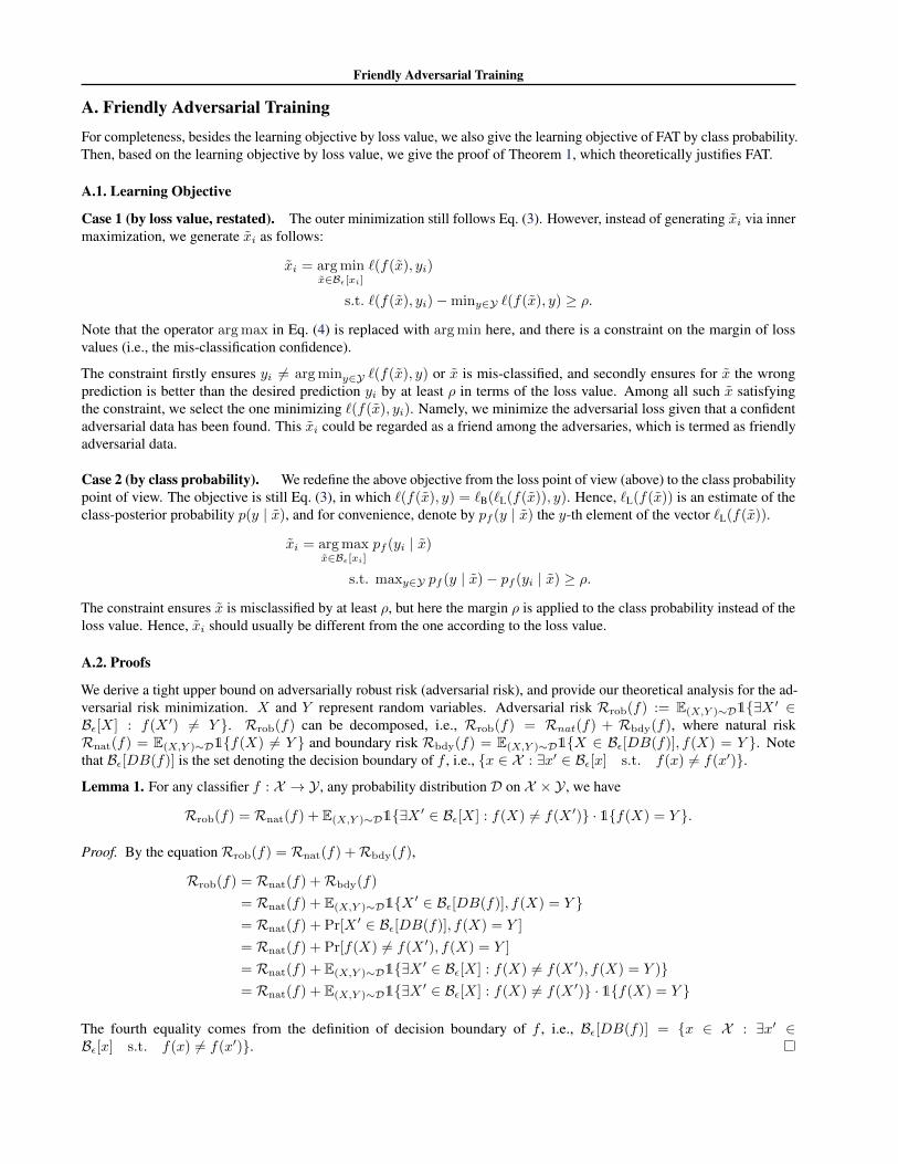
Minimizing 𝑅"#$
Figure 8. Solid line is the classifier. The area between dashed line is decision boundary of the classifier. Minimizing robust risk Rrob is tofind a classifier, where data is less likely located within decision boundary of the classifier.
Figure 8 illustrates the message of Lemma 1. Minimizing robust risk Rrob encourages the learning algorithm to find aclassifier whose decision boundary contains less training data. Meanwhile, the classifier should correctly separate data fromdifferent classes. Finding such a classifier is hard. As we can see in Figure 8, the hypothesis set of hyperplanes is enough forminimizing the natural risk (the left figure). However, a robust classifier (the right figure) has much curvatures, which ismore complicated. Nakkiran (2019) states that robust classification needs more complex classifiers (exponentially morecomplex, in some examples). This implies that in order to learn a robust classifier, our learning algorithm needs (a) setting alarge hypothesis set and (b) fine-tuning the decision boundary.
Theorem 1 (restated). For any classifier f , any non-negative surrogate loss function ` which upper bounds 0/1 loss, andany probability distribution D, we have
Rrob(f) ≤ E(X,Y )∼D`(f(X), Y )︸ ︷︷ ︸For standard test accuracy
+ E(X,Y )∼D,X′∈Bε[X,ε]`∗(f(X ′), Y )︸ ︷︷ ︸
For robust test accuracy
,
where
`∗ =
{min `(f(X ′), Y ) + ρ, if f(X ′) 6= Y ;
max `(f(X ′), Y ), if f(X ′) = Y.
ρ is the small constant.
Friendly Adversarial Training
Proof.
Rrob(f) = Rnat(f) +Rbdy(f)
≤ E(X,Y )∼D`(f(X), Y ) +Rbdy(f)
= E(X,Y )∼D`(f(X), Y ) + E(X,Y )∼D1{X ∈ Bε[DB(f)], f(X) = Y }= E(X,Y )∼D`(f(X), Y ) + Pr[X ∈ Bε[DB(f)], f(X) = Y ]
= E(X,Y )∼D`(f(X), Y ) + Pr[f(X) 6= f(X ′), f(X) = Y ]
≤ E(X,Y )∼D`(f(X), Y ) + Pr[f(X ′) 6= Y ]
= E(X,Y )∼D`(f(X), Y ) + E(X,Y )∼D1{∃X ′ ∈ Bε[X] : f(X ′) 6= Y }≤ E(X,Y )∼D`(f(X), Y ) + E(X,Y )∼D,X′∈Bε[X,ε]`
∗(f(X ′), Y )
The first inequality comes from the assumption that surrogate loss function ` upper bound 0/1 loss function. The secondinequality comes from the fact that there exists misclassified natural data within the decision boundary set. Therefore,Pr[f(X) 6= f(X ′), f(X) = Y ] ∪ Pr[f(X) 6= f(X ′), f(X) 6= Y ] = Pr[f(X ′) 6= Y ]. The third inequality comes from theassumption that surrogate loss function ` upper bound 0/1 loss function, i.e., in Figure 2, the adversarial data X ′ (purpletriangle) is on line of logistic loss (blue line), which is always above the 0/1 loss (yellow line).
Our Theorem 1 informs our strategy to fine tune the decision boundary. To fine-tune the decision boundary, the data “near”the classifier plays an important role. Those data are easily wrongly predicted with small perturbations. As we show in theFigure 2, when adversarial data are wrongly predicted, our adversarial data (purple triangle) increases to minimize the lossby a violation of a small constant ρ. Thus, our adversarial data can help fine-tune the decision boundary “bit by bit” over thetraining.
B. Alternative Adversarial Data Searching AlgorithmIn this section, we give an alternative adversarial data searching algorithm to generate friendly adversarial data via modifyingthe method to update x in Algorithm 1. We remove the constraint of ε-ball projection in Eq. (5), i.e.,
x(t+1) = x(t) + α sign(∇x(t)`(fθ(x(t)), y)),∀t ≥ 0 (6)
where x0 is a natural data and α > 0 is step size.
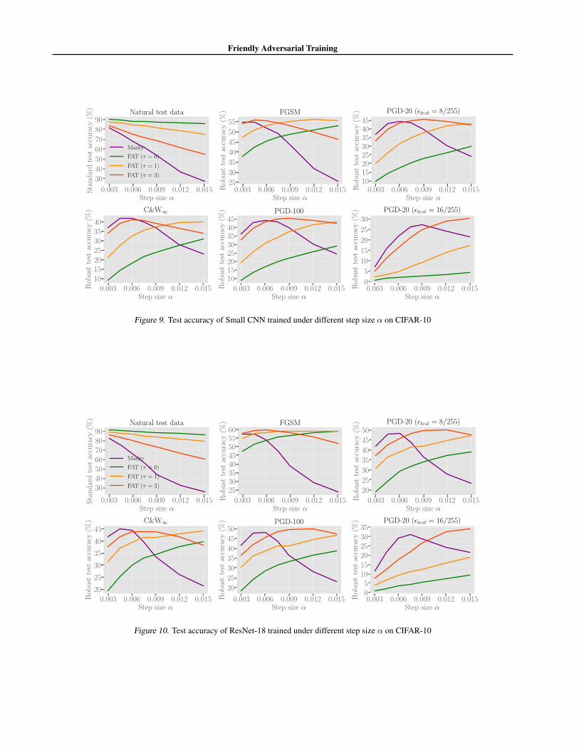
We employ Small CNN and ResNet-18 to show the performance of deep models against FGSM, PGD-20, PGD-100 andC&W∞ in Figure 9 and Figure 10. Deep models are trained using SGD with 0.9 momentum for 80 epochs with the initiallearning rate 0.01 divided by 10 at 60 epoch. We compare FAT combined with the alternative adversarial data searchingalgorithm (τ = 0, 1, 3) and standard adversarial training (Madry) with different step size α, i.e., α ∈ [0.003, 0.015]. Themaximum PGD step K is fixed to 10. All the testing settings are the same as those are stated in Section 6.1.
Friendly Adversarial Training
0.003 0.006 0.009 0.012 0.015Step size α
30
40
50
60
70
80
90
Sta
nd
ard
test
accu
racy
(%)
Natural test data
Madry
FAT (τ = 0)
FAT (τ = 1)
FAT (τ = 3)
0.003 0.006 0.009 0.012 0.015Step size α
25
30
35
40
45
50
55
Rob
ust
test
accu
racy
(%) FGSM
0.003 0.006 0.009 0.012 0.015Step size α
1015202530354045
Rob
ust
test
accu
racy
(%) PGD-20 (εtest = 8/255)
0.003 0.006 0.009 0.012 0.015Step size α
10152025303540
Rob
ust
test
accu
racy
(%) C&W∞
0.003 0.006 0.009 0.012 0.015Step size α
1015202530354045
Rob
ust
test
accu
racy
(%) PGD-100
0.003 0.006 0.009 0.012 0.015Step size α
0
5
10
15
20
25
30
Rob
ust
test
accu
racy
(%) PGD-20 (εtest = 16/255)
Figure 9. Test accuracy of Small CNN trained under different step size α on CIFAR-10
0.003 0.006 0.009 0.012 0.015Step size α
30405060708090
Sta
nd
ard
test
accu
racy
(%)
Natural test data
Madry
FAT (τ = 0)
FAT (τ = 1)
FAT (τ = 3)
0.003 0.006 0.009 0.012 0.015Step size α
2530354045505560
Rob
ust
test
accu
racy
(%) FGSM
0.003 0.006 0.009 0.012 0.015Step size α
20
25
30
35
40
45
50
Rob
ust
test
accu
racy
(%) PGD-20 (εtest = 8/255)
0.003 0.006 0.009 0.012 0.015Step size α
20
25
30
35
40
45
Rob
ust
test
accu
racy
(%) C&W∞
0.003 0.006 0.009 0.012 0.015Step size α
20
25
30
35
40
45
50
Rob
ust
test
accu
racy
(%) PGD-100
0.003 0.006 0.009 0.012 0.015Step size α
05
101520253035
Rob
ust
test
accu
racy
(%) PGD-20 (εtest = 16/255)
Figure 10. Test accuracy of ResNet-18 trained under different step size α on CIFAR-10
Friendly Adversarial Training
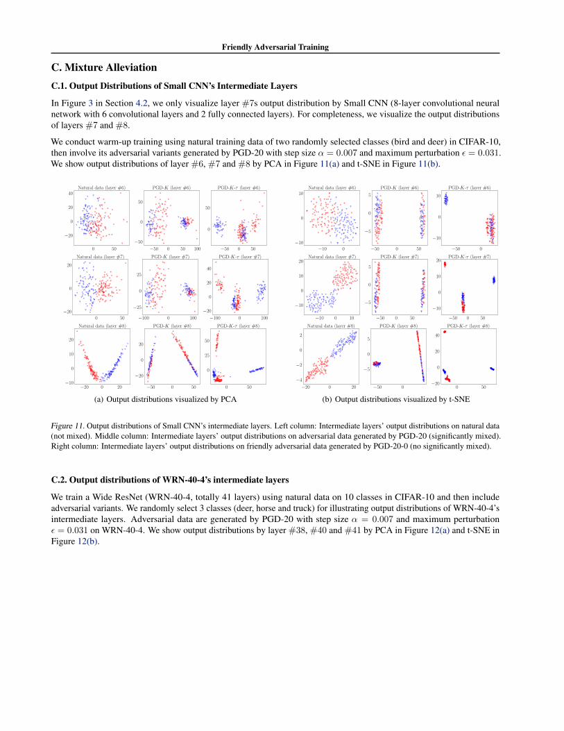
C. Mixture AlleviationC.1. Output Distributions of Small CNN’s Intermediate Layers
In Figure 3 in Section 4.2, we only visualize layer #7s output distribution by Small CNN (8-layer convolutional neuralnetwork with 6 convolutional layers and 2 fully connected layers). For completeness, we visualize the output distributionsof layers #7 and #8.
We conduct warm-up training using natural training data of two randomly selected classes (bird and deer) in CIFAR-10,then involve its adversarial variants generated by PGD-20 with step size α = 0.007 and maximum perturbation ε = 0.031.We show output distributions of layer #6, #7 and #8 by PCA in Figure 11(a) and t-SNE in Figure 11(b).
0 50
−20
0
20
40Natural data (layer #6)
−50 0 50 100
−50
0
50
PGD-K (layer #6)
−50 0 50
0
50
PGD-K-τ (layer #6)
0 50
−20
0
20
Natural data (layer #7)
−100 0 100
−25
0
25
PGD-K (layer #7)
−100 0 100
−20
0
20
40
PGD-K-τ (layer #7)
−20 0 20−10
0
10
20
Natural data (layer #8)
−50 0 50
−20
0
20
PGD-K (layer #8)
0 50
0
25
50
PGD-K-τ (layer #8)
(a) Output distributions visualized by PCA
−10 0−10
0
10Natural data (layer #6)
−50 0 50
−5
0
5
PGD-K (layer #6)
−50 0
−10
0
10
PGD-K-τ (layer #6)
−10 0 10
−10
0
10
20Natural data (layer #7)
−50 0 50
−5
0
5
PGD-K (layer #7)
−50 0 50
−10
0
10
20PGD-K-τ (layer #7)
−20 0 20
−4
−2
0
2
Natural data (layer #8)
−50 0
−5
0
5
PGD-K (layer #8)
0 50−20
0
20
40
PGD-K-τ (layer #8)
(b) Output distributions visualized by t-SNE
Figure 11. Output distributions of Small CNN’s intermediate layers. Left column: Intermediate layers’ output distributions on natural data(not mixed). Middle column: Intermediate layers’ output distributions on adversarial data generated by PGD-20 (significantly mixed).Right column: Intermediate layers’ output distributions on friendly adversarial data generated by PGD-20-0 (no significantly mixed).
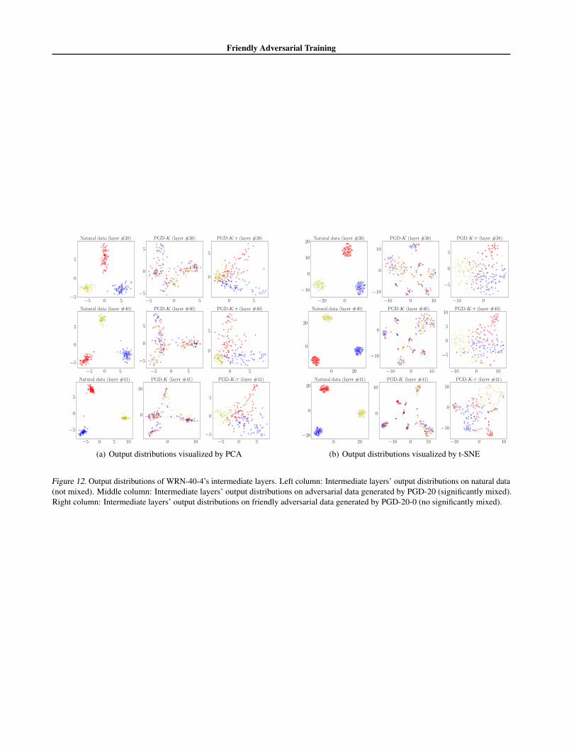
C.2. Output distributions of WRN-40-4’s intermediate layers
We train a Wide ResNet (WRN-40-4, totally 41 layers) using natural data on 10 classes in CIFAR-10 and then includeadversarial variants. We randomly select 3 classes (deer, horse and truck) for illustrating output distributions of WRN-40-4’sintermediate layers. Adversarial data are generated by PGD-20 with step size α = 0.007 and maximum perturbationε = 0.031 on WRN-40-4. We show output distributions by layer #38, #40 and #41 by PCA in Figure 12(a) and t-SNE inFigure 12(b).
Friendly Adversarial Training
−5 0 5−5
0
5
Natural data (layer #38)
−5 0 5
−5
0
5
PGD-K (layer #38)
0 5
0
5
PGD-K-τ (layer #38)
−5 0 5
−5
0
5
Natural data (layer #40)
−5 0 5
−5
0
5
PGD-K (layer #40)
0 5
0
5
PGD-K-τ (layer #40)
−5 0 5 10
−5
0
5
Natural data (layer #41)
0 10
0
10
PGD-K (layer #41)
−5 0 5
−5
0
5
PGD-K-τ (layer #41)
(a) Output distributions visualized by PCA
−20 0
−10
0
10
20Natural data (layer #38)
−10 0 10
−10
0
10
PGD-K (layer #38)
−10 0
−5
0
5
PGD-K-τ (layer #38)
0 20
0
20
Natural data (layer #40)
−10 0 10
−10
0
PGD-K (layer #40)
−10 0 10
−5
0
5
10PGD-K-τ (layer #40)
0 20
−20
0
20
Natural data (layer #41)
−10 0 10
0
10
PGD-K (layer #41)
−10 0 10
−10
0
10
PGD-K-τ (layer #41)
(b) Output distributions visualized by t-SNE
Figure 12. Output distributions of WRN-40-4’s intermediate layers. Left column: Intermediate layers’ output distributions on natural data(not mixed). Middle column: Intermediate layers’ output distributions on adversarial data generated by PGD-20 (significantly mixed).Right column: Intermediate layers’ output distributions on friendly adversarial data generated by PGD-20-0 (no significantly mixed).

Friendly Adversarial Training
D. FAT for TRADESD.1. Learning Objective of TRADES
Besides the standard adversarial training, TRADES is another effective adversarial training method (Zhang et al., 2019b),which trains on both natural data x and adversarial data x.
Similar to virtual adversarial training (VAT) adding a regularization term to the loss function (Miyato et al., 2016), whichregularizes the output distribution by its local sensitivity of the output w.r.t. input, the objective of TRADES is
minf∈F
1
n
n∑i=1
{`(f(xi), yi) + β`KL(f(xi), f(xi))
}, (7)
where β > 0 is a regularization parameter, which controls the trade-off between standard accuracy and robustness accuracy,i.e., as β increases, standard accuracy will decease while robustness accuracy will increase, and vice visa. Meanwhile, xi inTRADES is dynamically generated by
xi = arg maxx∈Bε[xi] `KL(f(x), f(x)), (8)
and `KL is Kullback-Leibler loss that is calculated by
`KL(f(x), f(x)) =
C∑i=1
`iL(f(x)) log
(`iL(f(x))
`iL(f(x))
).
D.2. FAT for TRADES - Realization
Algorithm 3 PGD-K-τ (Early Stopped PGD for TRADES)Input: data x ∈ X , label y ∈ Y , model f , loss function `KL, maximum PGD step K, step τ , perturbation bound ε, stepsize αOutput: xx← x+ ξN (0, I)while K > 0 do
if arg maxi f(x) 6= y and τ = 0 thenbreak
else if arg maxi f(x) 6= y thenτ ← τ − 1
end ifx← ΠB[x,ε]
(α sign(∇x`KL(f(x), f(x)) + x
)K ← K − 1
end while
In Algorithm 3, N (0, I) generates a random unit vector of d dimension. ξ is a small constant. `KL is Kullback-Leibler loss.
Given a dataset S = {(xi, yi)}ni=1, where xi ∈ Rd and yi ∈ {0, 1, ..., C − 1}, adversarial training (TRADES) with earlystopped PGD-K-τ returns a classifier θ∗:
θ∗ = arg minθ
n∑i=1
{`CE(fθ(xi), yi) + β`KL(fθ(xi), fθ(xi))
}(9)
where fθ : Rd → RC is DNN classification function, fθ(·) outputs predicted probability over C classes, The adversarialdata xi of xi is dynamically generated according to Algorithm 3, β > 0 is a regularization parameter, `CE is cross-entropyloss, `KL is Kullback-Leibler loss.
Based on our early stopped PGD-K-τ for TRADES in Algorithm 3, our friendly adversarial training for TRADES (FAT forTRADES) is
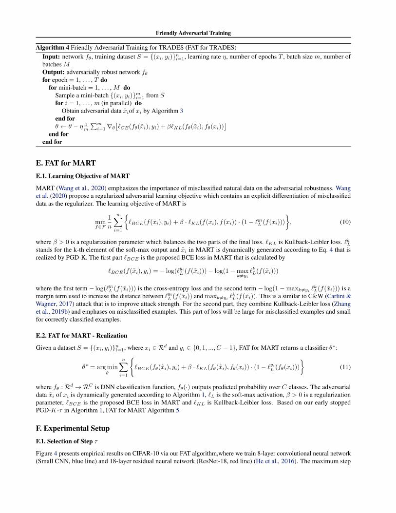
Friendly Adversarial Training
Algorithm 4 Friendly Adversarial Training for TRADES (FAT for TRADES)Input: network fθ, training dataset S = {(xi, yi)}ni=1, learning rate η, number of epochs T , batch size m, number ofbatches MOutput: adversarially robust network fθfor epoch = 1, . . . , T do
for mini-batch = 1, . . . , M doSample a mini-batch {(xi, yi)}mi=1 from Sfor i = 1, . . . , m (in parallel) do
Obtain adversarial data xiof xi by Algorithm 3end forθ ← θ − η 1
m
∑mi−1∇θ
[`CE(fθ(xi), yi) + β`KL(fθ(xi), fθ(xi))
]end for
end for
E. FAT for MARTE.1. Learning Objective of MART
MART (Wang et al., 2020) emphasizes the importance of misclassified natural data on the adversarial robustness. Wanget al. (2020) propose a regularized adversarial learning objective which contains an explicit differentiation of misclassifieddata as the regularizer. The learning objective of MART is
minf∈F
1
n
n∑i=1
{`BCE(f(xi), yi) + β · `KL(f(xi), f(xi)) · (1− `yiL (f(xi)))
}, (10)
where β > 0 is a regularization parameter which balances the two parts of the final loss. `KL is Kullback-Leibler loss. `kLstands for the k-th element of the soft-max output and xi in MART is dynamically generated according to Eq. 4 that isrealized by PGD-K. The first part `BCE is the proposed BCE loss in MART that is calculated by
`BCE(f(xi), yi) = − log(`yiL (f(xi)))− log(1−maxk 6=yi
`kL(f(xi)))
where the first term − log(`yiL (f(xi))) is the cross-entropy loss and the second term − log(1 −maxk 6=yi `kL(f(xi))) is a
margin term used to increase the distance between `yiL (f(xi)) and maxk 6=yi `kL(f(xi)). This is a similar to C&W (Carlini &
Wagner, 2017) attack that is to improve attack strength. For the second part, they combine Kullback-Leibler loss (Zhanget al., 2019b) and emphases on misclassified examples. This part of loss will be large for misclassified examples and smallfor correctly classified examples.
E.2. FAT for MART - Realization
Given a dataset S = {(xi, yi)}ni=1, where xi ∈ Rd and yi ∈ {0, 1, ..., C − 1}, FAT for MART returns a classifier θ∗:
θ∗ = arg minθ
n∑i=1
{`BCE(fθ(xi), yi) + β · `KL(fθ(xi), fθ(xi)) · (1− `yiL (fθ(xi)))
}(11)
where fθ : Rd → RC is DNN classification function, fθ(·) outputs predicted probability over C classes. The adversarialdata xi of xi is dynamically generated according to Algorithm 1, `L is the soft-max activation, β > 0 is a regularizationparameter, `BCE is the proposed BCE loss in MART and `KL is Kullback-Leibler loss. Based on our early stoppedPGD-K-τ in Algorithm 1, FAT for MART Algorithm 5.
F. Experimental SetupF.1. Selection of Step τ
Figure 4 presents empirical results on CIFAR-10 via our FAT algorithm,where we train 8-layer convolutional neural network(Small CNN, blue line) and 18-layer residual neural network (ResNet-18, red line) (He et al., 2016). The maximum step
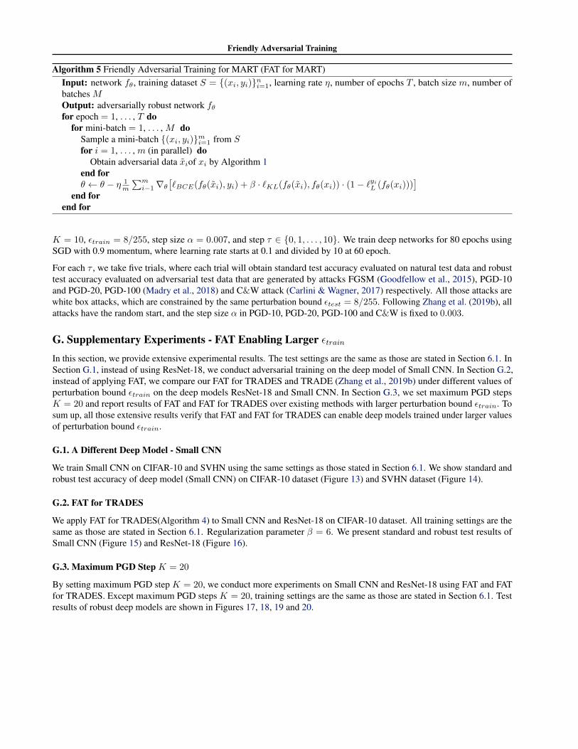
Friendly Adversarial Training
Algorithm 5 Friendly Adversarial Training for MART (FAT for MART)Input: network fθ, training dataset S = {(xi, yi)}ni=1, learning rate η, number of epochs T , batch size m, number ofbatches MOutput: adversarially robust network fθfor epoch = 1, . . . , T do
for mini-batch = 1, . . . , M doSample a mini-batch {(xi, yi)}mi=1 from Sfor i = 1, . . . , m (in parallel) do
Obtain adversarial data xiof xi by Algorithm 1end forθ ← θ − η 1
m
∑mi−1∇θ
[`BCE(fθ(xi), yi) + β · `KL(fθ(xi), fθ(xi)) · (1− `yiL (fθ(xi)))
]end for
end for
K = 10, εtrain = 8/255, step size α = 0.007, and step τ ∈ {0, 1, . . . , 10}. We train deep networks for 80 epochs usingSGD with 0.9 momentum, where learning rate starts at 0.1 and divided by 10 at 60 epoch.
For each τ , we take five trials, where each trial will obtain standard test accuracy evaluated on natural test data and robusttest accuracy evaluated on adversarial test data that are generated by attacks FGSM (Goodfellow et al., 2015), PGD-10and PGD-20, PGD-100 (Madry et al., 2018) and C&W attack (Carlini & Wagner, 2017) respectively. All those attacks arewhite box attacks, which are constrained by the same perturbation bound εtest = 8/255. Following Zhang et al. (2019b), allattacks have the random start, and the step size α in PGD-10, PGD-20, PGD-100 and C&W is fixed to 0.003.
G. Supplementary Experiments - FAT Enabling Larger εtrain
In this section, we provide extensive experimental results. The test settings are the same as those are stated in Section 6.1. InSection G.1, instead of using ResNet-18, we conduct adversarial training on the deep model of Small CNN. In Section G.2,instead of applying FAT, we compare our FAT for TRADES and TRADE (Zhang et al., 2019b) under different values ofperturbation bound εtrain on the deep models ResNet-18 and Small CNN. In Section G.3, we set maximum PGD stepsK = 20 and report results of FAT and FAT for TRADES over existing methods with larger perturbation bound εtrain. Tosum up, all those extensive results verify that FAT and FAT for TRADES can enable deep models trained under larger valuesof perturbation bound εtrain.
G.1. A Different Deep Model - Small CNN
We train Small CNN on CIFAR-10 and SVHN using the same settings as those stated in Section 6.1. We show standard androbust test accuracy of deep model (Small CNN) on CIFAR-10 dataset (Figure 13) and SVHN dataset (Figure 14).
G.2. FAT for TRADES
We apply FAT for TRADES(Algorithm 4) to Small CNN and ResNet-18 on CIFAR-10 dataset. All training settings are thesame as those are stated in Section 6.1. Regularization parameter β = 6. We present standard and robust test results ofSmall CNN (Figure 15) and ResNet-18 (Figure 16).
G.3. Maximum PGD Step K = 20
By setting maximum PGD step K = 20, we conduct more experiments on Small CNN and ResNet-18 using FAT and FATfor TRADES. Except maximum PGD steps K = 20, training settings are the same as those are stated in Section 6.1. Testresults of robust deep models are shown in Figures 17, 18, 19 and 20.
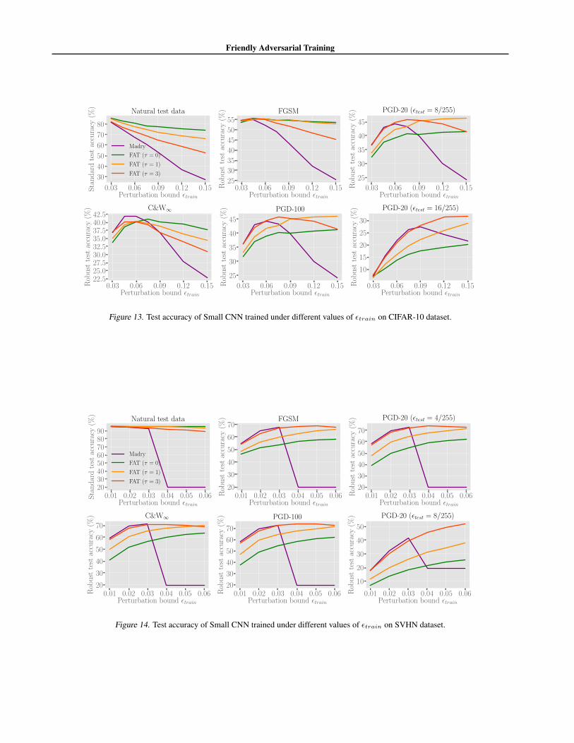
Friendly Adversarial Training
0.03 0.06 0.09 0.12 0.15Perturbation bound εtrain
30
40
50
60
70
80
Sta
nd
ard
test
accu
racy
(%)
Natural test data
Madry
FAT (τ = 0)
FAT (τ = 1)
FAT (τ = 3)
0.03 0.06 0.09 0.12 0.15Perturbation bound εtrain
25
30
35
40
45
50
55
Rob
ust
test
accu
racy
(%) FGSM
0.03 0.06 0.09 0.12 0.15Perturbation bound εtrain
25
30
35
40
45
Rob
ust
test
accu
racy
(%) PGD-20 (εtest = 8/255)
0.03 0.06 0.09 0.12 0.15Perturbation bound εtrain
22.525.027.530.032.535.037.540.042.5
Rob
ust
test
accu
racy
(%) C&W∞
0.03 0.06 0.09 0.12 0.15Perturbation bound εtrain
25
30
35
40
45R
obu
stte
stac
cura
cy(%
) PGD-100
0.03 0.06 0.09 0.12 0.15Perturbation bound εtrain
10
15
20
25
30
Rob
ust
test
accu
racy
(%) PGD-20 (εtest = 16/255)
Figure 13. Test accuracy of Small CNN trained under different values of εtrain on CIFAR-10 dataset.
0.01 0.02 0.03 0.04 0.05 0.06Perturbation bound εtrain
2030405060708090
Sta
nd
ard
test
accu
racy
(%)
Natural test data
Madry
FAT (τ = 0)
FAT (τ = 1)
FAT (τ = 3)
0.01 0.02 0.03 0.04 0.05 0.06Perturbation bound εtrain
20
30
40
50
60
70
Rob
ust
test
accu
racy
(%) FGSM
0.01 0.02 0.03 0.04 0.05 0.06Perturbation bound εtrain
20
30
40
50
60
70
Rob
ust
test
accu
racy
(%) PGD-20 (εtest = 4/255)
0.01 0.02 0.03 0.04 0.05 0.06Perturbation bound εtrain
20
30
40
50
60
70
Rob
ust
test
accu
racy
(%) C&W∞
0.01 0.02 0.03 0.04 0.05 0.06Perturbation bound εtrain
20
30
40
50
60
70
Rob
ust
test
accu
racy
(%) PGD-100
0.01 0.02 0.03 0.04 0.05 0.06Perturbation bound εtrain
10
20
30
40
50
Rob
ust
test
accu
racy
(%) PGD-20 (εtest = 8/255)
Figure 14. Test accuracy of Small CNN trained under different values of εtrain on SVHN dataset.
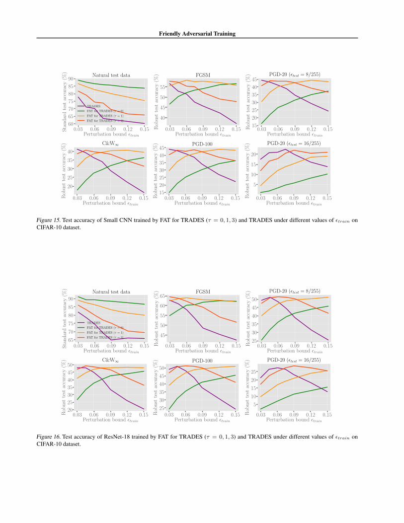
Friendly Adversarial Training
0.03 0.06 0.09 0.12 0.15Perturbation bound εtrain
60
65
70
75
80
85
90
Sta
nd
ard
test
accu
racy
(%)
Natural test data
TRADES
FAT for TRADES (τ = 0)
FAT for TRADES (τ = 1)
FAT for TRADES (τ = 3)
0.03 0.06 0.09 0.12 0.15Perturbation bound εtrain
40
45
50
55
Rob
ust
test
accu
racy
(%) FGSM
0.03 0.06 0.09 0.12 0.15Perturbation bound εtrain
15
20
25
30
35
40
45
Rob
ust
test
accu
racy
(%) PGD-20 (εtest = 8/255)
0.03 0.06 0.09 0.12 0.15Perturbation bound εtrain
20
25
30
35
40
Rob
ust
test
accu
racy
(%) C&W∞
0.03 0.06 0.09 0.12 0.15Perturbation bound εtrain
15
20
25
30
35
40
45
Rob
ust
test
accu
racy
(%) PGD-100
0.03 0.06 0.09 0.12 0.15Perturbation bound εtrain
5
10
15
20
Rob
ust
test
accu
racy
(%) PGD-20 (εtest = 16/255)
Figure 15. Test accuracy of Small CNN trained by FAT for TRADES (τ = 0, 1, 3) and TRADES under different values of εtrain onCIFAR-10 dataset.
0.03 0.06 0.09 0.12 0.15Perturbation bound εtrain
65
70
75
80
85
90
Sta
nd
ard
test
accu
racy
(%)
Natural test data
TRADES
FAT for TRADES (τ = 0)
FAT for TRADES (τ = 1)
FAT for TRADES (τ = 3)
0.03 0.06 0.09 0.12 0.15Perturbation bound εtrain
45
50
55
60
65
Rob
ust
test
accu
racy
(%) FGSM
0.03 0.06 0.09 0.12 0.15Perturbation bound εtrain
25
30
35
40
45
50
Rob
ust
test
accu
racy
(%) PGD-20 (εtest = 8/255)
0.03 0.06 0.09 0.12 0.15Perturbation bound εtrain
20
25
30
35
40
45
50
Rob
ust
test
accu
racy
(%) C&W∞
0.03 0.06 0.09 0.12 0.15Perturbation bound εtrain
25
30
35
40
45
50
Rob
ust
test
accu
racy
(%) PGD-100
0.03 0.06 0.09 0.12 0.15Perturbation bound εtrain
5
10
15
20
25
Rob
ust
test
accu
racy
(%) PGD-20 (εtest = 16/255)
Figure 16. Test accuracy of ResNet-18 trained by FAT for TRADES (τ = 0, 1, 3) and TRADES under different values of εtrain onCIFAR-10 dataset.
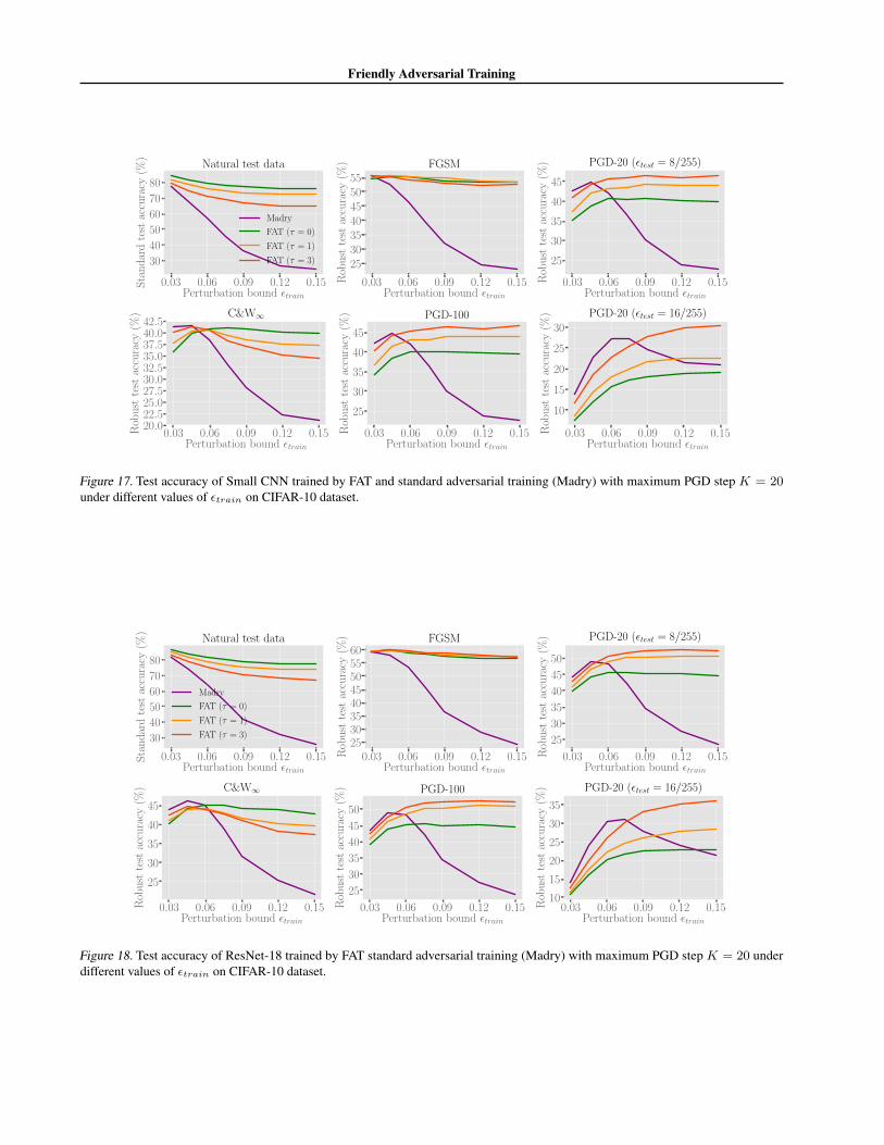
Friendly Adversarial Training
0.03 0.06 0.09 0.12 0.15Perturbation bound εtrain
30
40
50
60
70
80
Sta
nd
ard
test
accu
racy
(%)
Natural test data
Madry
FAT (τ = 0)
FAT (τ = 1)
FAT (τ = 3)
0.03 0.06 0.09 0.12 0.15Perturbation bound εtrain
25303540455055
Rob
ust
test
accu
racy
(%) FGSM
0.03 0.06 0.09 0.12 0.15Perturbation bound εtrain
25
30
35
40
45
Rob
ust
test
accu
racy
(%) PGD-20 (εtest = 8/255)
0.03 0.06 0.09 0.12 0.15Perturbation bound εtrain
20.022.525.027.530.032.535.037.540.042.5
Rob
ust
test
accu
racy
(%) C&W∞
0.03 0.06 0.09 0.12 0.15Perturbation bound εtrain
25
30
35
40
45R
obu
stte
stac
cura
cy(%
) PGD-100
0.03 0.06 0.09 0.12 0.15Perturbation bound εtrain
10
15
20
25
30
Rob
ust
test
accu
racy
(%) PGD-20 (εtest = 16/255)
Figure 17. Test accuracy of Small CNN trained by FAT and standard adversarial training (Madry) with maximum PGD step K = 20under different values of εtrain on CIFAR-10 dataset.
0.03 0.06 0.09 0.12 0.15Perturbation bound εtrain
30
40
50
60
70
80
Sta
nd
ard
test
accu
racy
(%)
Natural test data
Madry
FAT (τ = 0)
FAT (τ = 1)
FAT (τ = 3)
0.03 0.06 0.09 0.12 0.15Perturbation bound εtrain
2530354045505560
Rob
ust
test
accu
racy
(%) FGSM
0.03 0.06 0.09 0.12 0.15Perturbation bound εtrain
25
30
35
40
45
50
Rob
ust
test
accu
racy
(%) PGD-20 (εtest = 8/255)
0.03 0.06 0.09 0.12 0.15Perturbation bound εtrain
25
30
35
40
45
Rob
ust
test
accu
racy
(%) C&W∞
0.03 0.06 0.09 0.12 0.15Perturbation bound εtrain
25
30
35
40
45
50
Rob
ust
test
accu
racy
(%) PGD-100
0.03 0.06 0.09 0.12 0.15Perturbation bound εtrain
10
15
20
25
30
35
Rob
ust
test
accu
racy
(%) PGD-20 (εtest = 16/255)
Figure 18. Test accuracy of ResNet-18 trained by FAT standard adversarial training (Madry) with maximum PGD step K = 20 underdifferent values of εtrain on CIFAR-10 dataset.
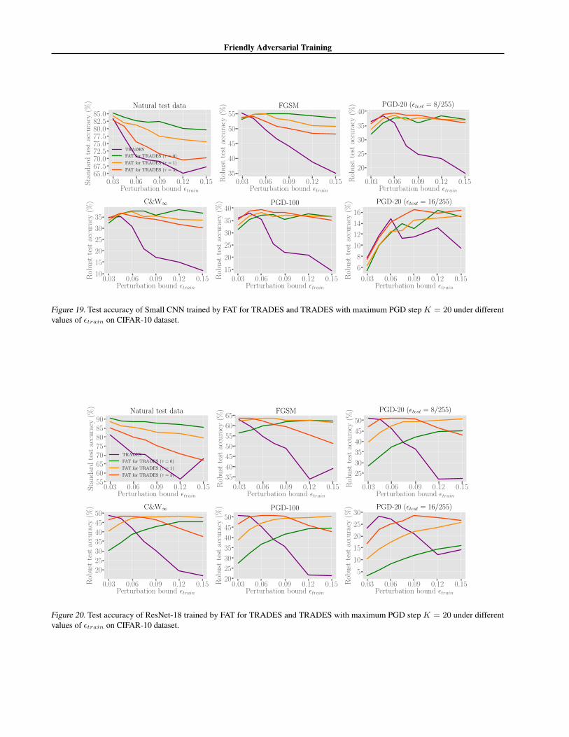
Friendly Adversarial Training
0.03 0.06 0.09 0.12 0.15Perturbation bound εtrain
65.067.570.072.575.077.580.082.585.0
Sta
nd
ard
test
accu
racy
(%)
Natural test data
TRADES
FAT for TRADES (τ = 0)
FAT for TRADES (τ = 1)
FAT for TRADES (τ = 3)
0.03 0.06 0.09 0.12 0.15Perturbation bound εtrain
35
40
45
50
55
Rob
ust
test
accu
racy
(%) FGSM
0.03 0.06 0.09 0.12 0.15Perturbation bound εtrain
20
25
30
35
40
Rob
ust
test
accu
racy
(%) PGD-20 (εtest = 8/255)
0.03 0.06 0.09 0.12 0.15Perturbation bound εtrain
10
15
20
25
30
35
Rob
ust
test
accu
racy
(%) C&W∞
0.03 0.06 0.09 0.12 0.15Perturbation bound εtrain
15
20
25
30
35
40
Rob
ust
test
accu
racy
(%) PGD-100
0.03 0.06 0.09 0.12 0.15Perturbation bound εtrain
6
8
10
12
14
16
Rob
ust
test
accu
racy
(%) PGD-20 (εtest = 16/255)
Figure 19. Test accuracy of Small CNN trained by FAT for TRADES and TRADES with maximum PGD step K = 20 under differentvalues of εtrain on CIFAR-10 dataset.
0.03 0.06 0.09 0.12 0.15Perturbation bound εtrain
5560657075808590
Sta
nd
ard
test
accu
racy
(%)
Natural test data
TRADES
FAT for TRADES (τ = 0)
FAT for TRADES (τ = 1)
FAT for TRADES (τ = 3)
0.03 0.06 0.09 0.12 0.15Perturbation bound εtrain
35
40
45
50
55
60
65
Rob
ust
test
accu
racy
(%) FGSM
0.03 0.06 0.09 0.12 0.15Perturbation bound εtrain
25
30
35
40
45
50
Rob
ust
test
accu
racy
(%) PGD-20 (εtest = 8/255)
0.03 0.06 0.09 0.12 0.15Perturbation bound εtrain
20253035404550
Rob
ust
test
accu
racy
(%) C&W∞
0.03 0.06 0.09 0.12 0.15Perturbation bound εtrain
20
25
30
35
40
45
50
Rob
ust
test
accu
racy
(%) PGD-100
0.03 0.06 0.09 0.12 0.15Perturbation bound εtrain
5
10
15
20
25
30
Rob
ust
test
accu
racy
(%) PGD-20 (εtest = 16/255)
Figure 20. Test accuracy of ResNet-18 trained by FAT for TRADES and TRADES with maximum PGD step K = 20 under differentvalues of εtrain on CIFAR-10 dataset.
Friendly Adversarial Training
G.4. C&W Attack Analysis
As is shown in Figure 6 along with Figure 13 in Section G.1, both standard adversarial training and friendly adversarialtraining do not perform well under C&W (Carlini & Wagner, 2017) attack with larger εtrain (e.g., εtrain > 0.075). Wediscuss the reasons for these phenomena.
C&W attack. Given x, we choose a target class t and then search for adversarial data x under C&W attack in the Lpmetric by solving
minimize ‖x− x‖p + c · h(x)
with h defined as
h(x) = max(maxi6=t
f(x)i − f(x)t,−κ).
The parameter c > 0 balances two parts of loss. κ > 0 encourages the solver to find adversarial data x that will be classifiedas class t with high confidence. Note that this paper follows the implementation of C&W∞ attack in (Cai et al., 2018)1 and(Wang et al., 2019)2 where they replace the cross-entropy loss with h(x) in PGD, i.e.,
xi = arg maxx∈Bε[xi](maxi 6=yi
f(x)i − f(x)yi − κ). (12)
Analysis. In Figure 6, with larger εtrain, the performance evaluated by PGD attacks increases, while performanceevaluated by C&W attack decreases. The reason is that C&W and PGD have different ways of generating adversarial dataaccording to Eq. (12) and Eq. (4) respectively. The two interactive methods search adversarial data in different directionsdue to gradients w.r.t. different loss. Therefore, the distributions of C&W and PGD adversarial data are inconsistent. Asperturbation bound εtrain increases, there are more PGD adversarial data generated within εtrain-ball. A DNN learned frommore PGD adversarial data becomes more defensive to PGD attacks, but this deep model may not effectively defend C&Wadversarial data.
1curriculum adversarial training GitHub2dynamic adversarial training GitHub
Friendly Adversarial Training
H. Extensive State-of-the-art Results on Wide ResNetH.1. Training Details of FAT on WRN-32-10
In Table 1, we compare our FAT with standard adversarial training (Madry), CAT (Cai et al., 2018) and DAT (Wang et al.,2019).
We use FAT (εtrain = 8/255 and 16/255 respectively) to train WRN-32-10 for 120 epochs using SGD with 0.9 momentum,and weight decay is 0.0002. Maximum PGD step is 10 and step size is fixed to 0.007. The initial learning rate is 0.1 reducedto 0.01, 0.001 and 0.0005 at epoch 60, 90 and 110. We set step τ = 0 initially and increase τ by one at epoch 50 and 90respectively. The maximum step K = 10. We report performance of the deep model at the last epoch. For fair comparison,in Table 1 we use the same test settings as those in DAT (Wang et al., 2019). Performance of robust deep model is evaluatedstandard test accuracy for natural data and robust test accuracy for adversarial data, that are generated by FGSM, PGD-20(20-steps PGD with random start), PGD-100 and C&W∞(L∞ version of C&W optimized by PGD-30).
All attacks have the same perturbation bound εtest = 0.031 and step size in PGD is α = εtest/4. The same as DAT (Wanget al., 2019), there is random start in PGD attack, i.e., uniformly random perturbations ([−εtest,+εtest]) added to naturaldata before PGD perturbations. We report the median test accuracy and its standard deviation over 5 repeated trails ofadversarial training in Table 1.
H.2. Training details of FAT for TRADES on Wide ResNet
In Table 2, we use FAT for TRADES (εtrain = 8/255 and 16/255 respectively) train WRN-34-10 by FAT for TRADES for85 epochs using SGD with 0.9 momentum and 0.0002 weight decay. Maximum PGD step K = 10 and step size α = 0.007.The initial learning rate is 0.1 and divided 10 at epoch 75. We set step τ = 0 initially and increased by one at epoch 30, 50and 70. Since TRADES has a trade-off parameter β, for fair comparison, our FAT for TRADES use the same β. In Table 2,we set β = 1 and 6 separately, which are endorsed by (Zhang et al., 2019b).
For fair comparison, we use the same test settings as those are stated in TRADES (Zhang et al., 2019b). All attacks have thesame perturbation bound εtest = 0.031 ( without random start), and step size α = 0.003, which is the same as stated inthe paper (Zhang et al., 2019b). Performance of robust deep model is evaluated standard test accuracy for natural data androbust test accuracy for adversarial data, that are generated by FGSM, PGD-20, PGD-100 and C&W∞(L∞ version of C&Woptimized by PGD-30). We report the median test accuracy and its standard deviation of the deep model at the last epochover 3 repeated trials of adversarial training in Table 2.
Fair comparison based on TRADES’s experimental setting. However, in TRADES’s experimental testing3, they userandom start before PGD perturbation that is deviated from the statements in the paper (Zhang et al., 2019b). For faircomparison, we also retest the robust deep models under PGD attacks with random start. We evaluate their publicly releasedrobust deep model4 WRN-34-10 and compare it with ours trained by FAT for TRADES. The test results are reported inTable 3.
FAT for TRADES on larger WRN-58-10. We employ Wide ResNet with larger capacity, i.e., WRN-58-10 to showour superior performance achieved by FAT for TRADES in Table 3. All the training settings are the same as details onWRN-34-10 in this section. The regularization parameter β is fixed to 6.0. All attacks have the same perturbation boundεtest = 0.031 and step size α = 0.003, which is the same as TRADES’s experimental setting. Robustness against FGSM,PGD-20(20-steps PGD with random start) and C&W∞ is reported in Table 3.
H.3. FAT for MART on Wide ResNet
We train WRN-34-10 by FAT for MART (εtrain = 8/255 and 16/255 respectively) using SGD with 0.9 momentum and0.0002 weight decay. Maximum PGD step K = 10 and step size α = 0.007. The initial learning rate is 0.1 and divided10 at epoch 60 and 90 respectively. We set step τ = 0 initially and increase τ by one at epoch 20, 40, 60 and 80. Theregularization parameter β is fixed to 6.0. The maximum step size K = 10.
3TRADES GitHub4TRADES’s pre-trained model
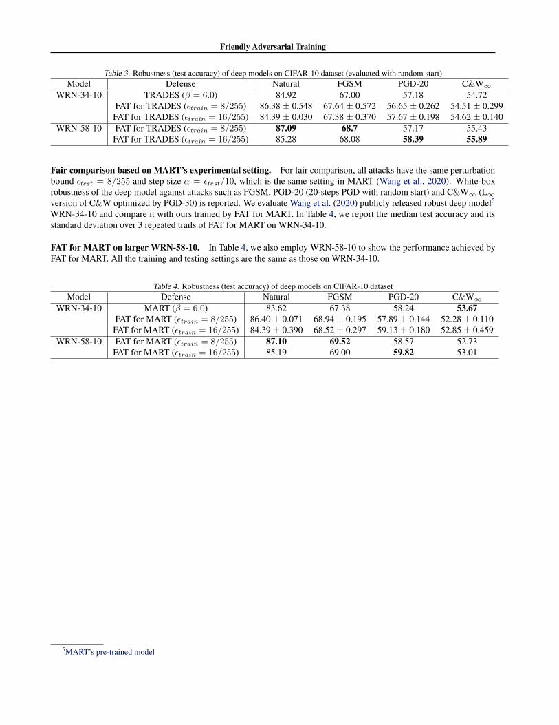
Friendly Adversarial Training
Table 3. Robustness (test accuracy) of deep models on CIFAR-10 dataset (evaluated with random start)Model Defense Natural FGSM PGD-20 C&W∞
WRN-34-10 TRADES (β = 6.0) 84.92 67.00 57.18 54.72FAT for TRADES (εtrain = 8/255) 86.38 ± 0.548 67.64 ± 0.572 56.65 ± 0.262 54.51 ± 0.299FAT for TRADES (εtrain = 16/255) 84.39 ± 0.030 67.38 ± 0.370 57.67 ± 0.198 54.62 ± 0.140
WRN-58-10 FAT for TRADES (εtrain = 8/255) 87.09 68.7 57.17 55.43FAT for TRADES (εtrain = 16/255) 85.28 68.08 58.39 55.89
Fair comparison based on MART’s experimental setting. For fair comparison, all attacks have the same perturbationbound εtest = 8/255 and step size α = εtest/10, which is the same setting in MART (Wang et al., 2020). White-boxrobustness of the deep model against attacks such as FGSM, PGD-20 (20-steps PGD with random start) and C&W∞ (L∞version of C&W optimized by PGD-30) is reported. We evaluate Wang et al. (2020) publicly released robust deep model5
WRN-34-10 and compare it with ours trained by FAT for MART. In Table 4, we report the median test accuracy and itsstandard deviation over 3 repeated trails of FAT for MART on WRN-34-10.
FAT for MART on larger WRN-58-10. In Table 4, we also employ WRN-58-10 to show the performance achieved byFAT for MART. All the training and testing settings are the same as those on WRN-34-10.
Table 4. Robustness (test accuracy) of deep models on CIFAR-10 datasetModel Defense Natural FGSM PGD-20 C&W∞
WRN-34-10 MART (β = 6.0) 83.62 67.38 58.24 53.67FAT for MART (εtrain = 8/255) 86.40 ± 0.071 68.94 ± 0.195 57.89 ± 0.144 52.28 ± 0.110FAT for MART (εtrain = 16/255) 84.39 ± 0.390 68.52 ± 0.297 59.13 ± 0.180 52.85 ± 0.459
WRN-58-10 FAT for MART (εtrain = 8/255) 87.10 69.52 58.57 52.73FAT for MART (εtrain = 16/255) 85.19 69.00 59.82 53.01
5MART’s pre-trained model