Attachment B Selenium QAPP

Lion Oil Company

Quality Assurance Project Plan for

Use Attainability Analysis of Loutre Creek

FINAL DRAFT March 25, 2009

Quality Assurance Project Plan for Use Attainability Analysis of Loutre Creek Prepared for: Lion Oil Company 1000 McHenry Ave El Dorado, AR 71730

Prepared by: GBMc & Associates 219 Brown Lane Bryant, AR 72022

FINAL DRAFT March 25, 2009

I. Project Management (Group A) Revision #1

3/25/09

I. PROJECT MANAGEMENT (GROUP A)

A1 Title and Approval Sheet

Title: Use Attainability Analysis of Loutre Creek Completed By: GBMc & Associates for Lion Oil, El Dorado, Arkansas

QAPP Approved by: Russell Nelson _________________ Water Quality Coordinator Signature EPA Region VI _________________ Date Sarah Clem _________________ Branch manager, Water Division Signature ADEQ _________________ Date Chuck Hammock _________________ Coordinator Signature Lion Oil _________________ Date Roland McDaniel _________________ Project manager Signature GBMc and Associates _________________ Date Greg Phillips. _________________ Quality Assurance Officer Signature GBMc and Associates _________________ Date Effective Date:____________________


3/25/09

A2 Table of Contents

I. PROJECT MANAGEMENT (GROUP A) Page A1 Title and Approval Sheet 1 A2 Table of Contents 2 A3 Distribution List 3 A4 Project/Task Organization 4 A5 Problem Definition/Background 6 A6 Project/Task Description 8 A7 Data Quality Objectives for Measurement Data 11 A8 Special Training Requirements/Certification 13 A9 Documentation and Records 14 II. DATA GENERATION AND ACQUISITION (GROUP B)

B1 Sampling Process Design 16 B2 Sampling Methods Requirements 19 B3 Sample Handling and Custody Requirements 25 B4 Analytical Methods Requirements 26 B5 Quality Control Requirements 27 B6 Instrument/Equipment Testing, Inspection, and

Maintenance Requirements 29

B7 Instrument Calibration and Frequency 30 B8 Inspection/Acceptance Requirements for Supplies and

Consumables 31

B9 Data Acquisition Requirements (Non-Direct Measurements) 32

1


3/25/09

B10 Data Management 33 III. ASSESSMENT AND OVERSIGHT (GROUP C) C1 Assessments and Response Actions 35 C2 Reports to Management 36 IV. DATA VALIDATION AND USEABILITY (GROUP D) D1 Data Review, Validation, and Verification Requirements 37 D2 Validation and Verification Methods 38 D3 Reconciliation with Data Quality Objectives 39

FIGURES

Figure 1. Organizational Chart...............................................................5

Figure 2. Sampling stations/Reaches for UAA .......................................7

TABLES

Table B1.1. Description of Sample Sections .......................................13

Table B1.2. Summary of Sample Design.............................................18

Table B2.1. Summary of Sampling Methods .......................................23

Table B2.2. Summary of Water Samples Taken for Analytical

Analysis for each Monitoring Period.................................24

Table B4.1. Summary of Analytical Methods.......................................26

Table B5.1. Summary of laboratory QA Requirements .......................28

Table B9.1. Summary of Use of Non-Direct Data (Existing)

Data in the Study..............................................................32

APPENDICES Appendix A - Selenium Data from Lion Oil Company Outfall 001 Appendix B - GBMc SOP Appendix C - Ana-Lab SOP’s

2


3/25/09

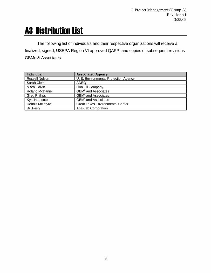
A3 Distribution List The following list of individuals and their respective organizations will receive a

finalized, signed, USEPA Region VI approved QAPP, and copies of subsequent revisions

GBMc & Associates:

Individual Associated Agency Russell Nelson U. S. Environmental Protection Agency Sarah Clem ADEQ Mitch Colvin Lion Oil Company Roland McDaniel GBMc and Associates Greg Phillips GBMc and Associates Kyle Hathcote GBMc and Associates Dennis McIntyre Great Lakes Environmental Center Bill Perry Ana-Lab Corporation

3


3/25/09

A4 Project/Task Organization

Russell Nelson USEPA Region VI USEPA Project Officer

Responsible for QAPP review & approval, and final report approval.

Sarah Clem Water Division ADEQ

Responsible for QAPP review & approval, and final report approval.

Mitch Colvin Lion Oil Project Coordinator

Responsible for project coordination

Roland McDaniel GBMc and Associates Project Manager

Responsible for project management

Greg Phillips GBMc and Associates Quality Assurance Officer

Responsible for adherence to QAPP

Kyle Hathcote GBMc and Associates Field Study Coordinator

Responsible for field studies and data collected from field studies

Dennis McIntyre Great Lakes Environmental Center Research Scientist

Responsible for selenium uptake and sub-lethal effects testing

Bill Perry Ana-Lab Corporation Lab Manager

Responsible for analytical lab analysis

4


3/25/09

Figure 1. Organizational chart.

5


3/25/09

A5 Problem Definition/Background Study Objective - The objective of the study is to complete a Use Attainability

Analysis (UAA) of Loutre Creek to determine if the system is fully supporting its fisheries

use, and if not, to develop a sub-category of the fisheries use that characterizes the

existing use and is consistent with the long term historical land uses of the watershed.

The sub-category fisheries use designation will then allow a site specific water quality

criterion to be developed for selenium through the 3rd party rule making process reflection

of the long term historical selenium concentrations of the receiving stream.

Background – Loutre Creek is a small sub-watershed (less the 4 mi2) to Bayou de

Loutre (less than 5 mi2 at the mouth of Loutre Creek) in Union county Arkansas that

drains the southern portion of the City of El Dorado (Figure 2.) The Loutre Creek

watershed is largely represented by oil field and industrial land-uses that have existed for

over 80 years. Lion Oil Company operates a refinery in the watershed and discharges

treated wastewater to Loutre Creek through NPDES Outfall 001 (NPDES No. AR000647).

Lion Oil is the only permitted discharger in the Loutre Creek Watershed.

During the most recent NPDES permit renewal, final permit limits for total selenium

at Outfall 001 was established as 5.8 micrograms per liter (µg/L) monthly average and

11.65µg/L daily maximum. The sampling during the interim period of the new permit

indicated the discharge from Outfall 001 would on occasion exceed the monthly maximum

concentration (Appendix A). This condition, in addition to other permit issues (e.g. final

zinc limitations, dissolved minerals rulemaking and storm water segregation project) led to

the development of the consent administrative order (CAO LIS No. 08-104). In

accordance with Item 3 of the CAO, Lion Oil developed a Compliance Action Plan that

outlined a plan of action to remedy the selenium compliance issue. One of the major

components of the CAP was to complete a UAA and develop site specific criteria (SSC)

for selenium in Loutre Creek and potentially in Bayou De Loutre.

6


3/25/09

7

Figure 2. Sample Stations/Reaches for the UAA.


3/25/09

A6 Project/Task Description The following tasks support the UAA and associated SSC development.

Task 1 - Biological Assessment

An biological assessment (bioassessment) will be completed to document the

existing conditions of the streams aquatic communities and physical habitat. Fish and

macroinvertebrate collections will be completed once during the spring season and once

during the summer season to assess the health of the biota and maintenance of biological

integrity. Detailed habitat assessment will be completed to document the available

habitat, the existing condition of the channel and the condition of the riparian corridor.

Fish will be collected using electro fishing techniques supplemented with seine hauls

where appropriate. Macroinvertebrates will be collected with kick nets using multi-habitat

protocols. All specimens will be identified to the lowest taxonomic level practicable.

Collections will be analyzed with several biometrics to determine community status. Data

generated during this Project will be compared to available historical data to evaluate

long-term trends in biological communities.

Task 2 - Toxicity Assessment

An evaluation of selenium toxicity will be completed to determine the effect of

selenium on resident biota from Loutre Creek. The assessment will focus on reproductive

and embryological effects to fishes in the Centrachidae (sunfish) family. Selenium levels

from the water column, sediment and within primary producer and primary consumer

trophic levels will be measured to develop a relationship between water column levels and

those affecting the test sunfish species.

Additionally, the historical Whole Effluent Toxicity (WET) test results completed as

a requirement of the NPDES permit will be reviewed and summarized to document that

the effluent from Outfall 001 has consistently PASSED biomonitoring at high critical

dilution requirements and the potential effects of selenium in those test results.

Task 3 - Chemical and In-Situ Analysis

8


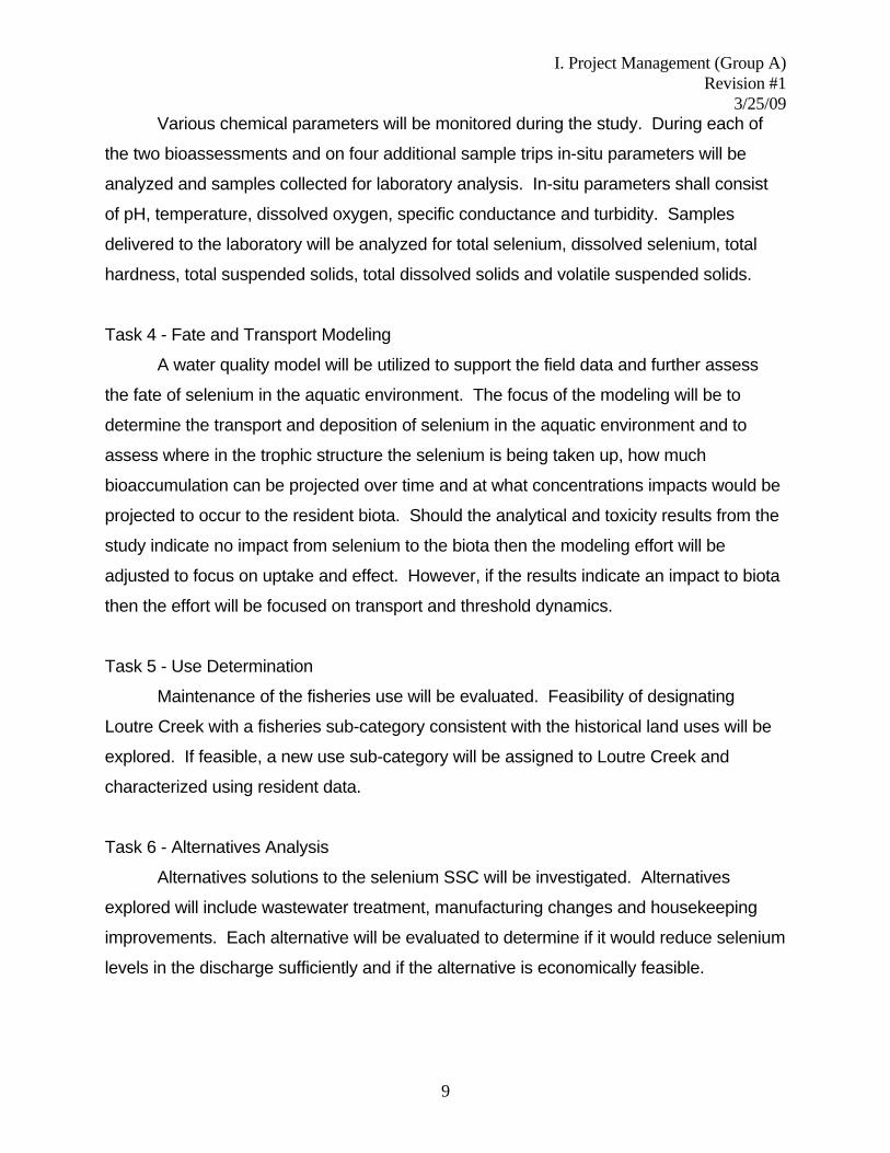
3/25/09 Various chemical parameters will be monitored during the study. During each of

the two bioassessments and on four additional sample trips in-situ parameters will be

analyzed and samples collected for laboratory analysis. In-situ parameters shall consist

of pH, temperature, dissolved oxygen, specific conductance and turbidity. Samples

delivered to the laboratory will be analyzed for total selenium, dissolved selenium, total

hardness, total suspended solids, total dissolved solids and volatile suspended solids.

Task 4 - Fate and Transport Modeling

A water quality model will be utilized to support the field data and further assess

the fate of selenium in the aquatic environment. The focus of the modeling will be to

determine the transport and deposition of selenium in the aquatic environment and to

assess where in the trophic structure the selenium is being taken up, how much

bioaccumulation can be projected over time and at what concentrations impacts would be

projected to occur to the resident biota. Should the analytical and toxicity results from the

study indicate no impact from selenium to the biota then the modeling effort will be

adjusted to focus on uptake and effect. However, if the results indicate an impact to biota

then the effort will be focused on transport and threshold dynamics.

Task 5 - Use Determination

Maintenance of the fisheries use will be evaluated. Feasibility of designating

Loutre Creek with a fisheries sub-category consistent with the historical land uses will be

explored. If feasible, a new use sub-category will be assigned to Loutre Creek and

characterized using resident data.

Task 6 - Alternatives Analysis

Alternatives solutions to the selenium SSC will be investigated. Alternatives

explored will include wastewater treatment, manufacturing changes and housekeeping

improvements. Each alternative will be evaluated to determine if it would reduce selenium

levels in the discharge sufficiently and if the alternative is economically feasible.

9


3/25/09 Task 7 - SSC Development

Upon assignment of the fisheries use sub-category to Loutre Creek a site SSC for

selenium will be developed for Loutre Creek. The SSC will be based on historical

selenium data from the stream and from Lion Oil Outfall 001.

Task 8 – Project Schedule A project schedule was developed for and adopted from the COA Lis No.08-10.

However, due to the protracted period required to finalize the CAO; the complex nature of

UAA documentation; field conditions; unforeseen natural occurrences, and extended

regulatory reviews, the ultimate project completion date may be modified. Any additional

modifications to the project schedule will be communicated as early in the process or

practicable.

Schedule:

Task No.

Task Description Start Date Completion Date

1 Biological Assessment February 1, 2009 October 30, 2009 2 Toxicity Assessment April 1, 2009 November 30, 2009 3 Chemical and in-Situ Analysis February 1, 2009 November 30, 2009 4 Fate and Transport Modeling May 1, 2009 November 30, 2009 5 Use Determination July 1, 2009 November 30, 2009 6 Alternative Analysis January 1, 2009 August 30, 2009 7 SSC Development November 30, 2009 May 2010 8 Deliverable - Draft

Report --- June 2010

9 Deliverable - Final Report --- July 2010

10


3/25/09

A7 Data Quality Objectives for Measurement Data Task 1 – Biological Assessment

Field teams collecting biota are led by experienced aquatic biologists and ecologists.

Field forms designed specifically for collection studies and set up to include all pertinent

field data are completed for each sample site. All field forms are reviewed at the end of

the study for completeness and accuracy. Identification of fish and macroinvertebrates is

verified in the laboratory by an experienced invertebrate biologist. Periodic spot checks to

verify laboratory identifications are made by a qualified biologist on the team. Collection

techniques are largely based on EPA bioassessment methodologies (Barbour, 1999) and

are considered comparable to results attained by other regional agencies, including the

ADEQ.

Representativeness and precision are measured for macroinvertebrate assessment

through collection of duplicate samples. Duplicate samples are collected at one of ten

study sites. One duplicate sample will be collected during each season (spring and

summer). A similarity index is calculated for the duplicate and base samples. Index

results indicating similarity less than 65% are suspect and require investigation.

Fish sampling equipment is routinely inspected to maintain and ensure proper working

order prior to a sampling trip. Electro shocking equipment is adjusted in the field to

ensure the most productive collection at each station. All available habitats are shocked

to ensure a representative sample is collected. Consistent level of effort (pedal down

time) is exerted at all stations to ensure results are comparable.

Task 2 – Toxicity Assessment

Routine WET testing has been completed following the EPA specific guidance for WET

testing (EPA-821-R-02-012 and EPA-821-R-02-013). Use of Quality Assurance

consistent with those guidelines and sufficient to meet DMR reporting requirements

provides an adequate level of data quality for this study and ensures data comparability.

Toxicity testing repeatability and precision is monitored through routine reference toxicity

testing. Reference toxicant endpoints should fall within the laboratory defined control

limits to ensure the test results are precise and repeatable. The completeness criteria for

11


3/25/09 the toxicity portion of the project is that 90% of the historical, testing results in data

meeting the data quality objectives.

Selenium reproductive and embryological effects testing will be completed consistent with

general EPA toxicity testing guidelines to ensure data is accurate and repeatable. That is,

test subjects (eggs and embryo-larval fish) will be tested in replicate, include controls,

utilize a reference condition, and test conditions will be monitored and controlled

according to specific guidelines. Toxicity endpoints (measures of toxic effects) will be

defined (see Section B4) specifically in this QAPP and strictly adhered to, to ensure

repeatability and limit bias.

Task 3 – Chemical and In-Situ Analysis

Sample collection techniques are based on those recommended by EPA for specific

media types in various guidance documents. Use of accepted methodology ensures that

the results are comparable. The completeness criteria for this project are that 90% of the

samples from each media provide usable results. That is, through the collection, handling

and analysis process there is an allowance that 10% of the samples (maximum) could be

lost, contaminated or rendered unusable due to field technician or laboratory error.

Representativeness of samples collected is assured by collecting a field duplicate

sample at a rate of 10% of samples collected, one per day of sampling, minimum.

Duplicates within +/- 20% of each other, are considered to prove the representativeness

of collection techniques.

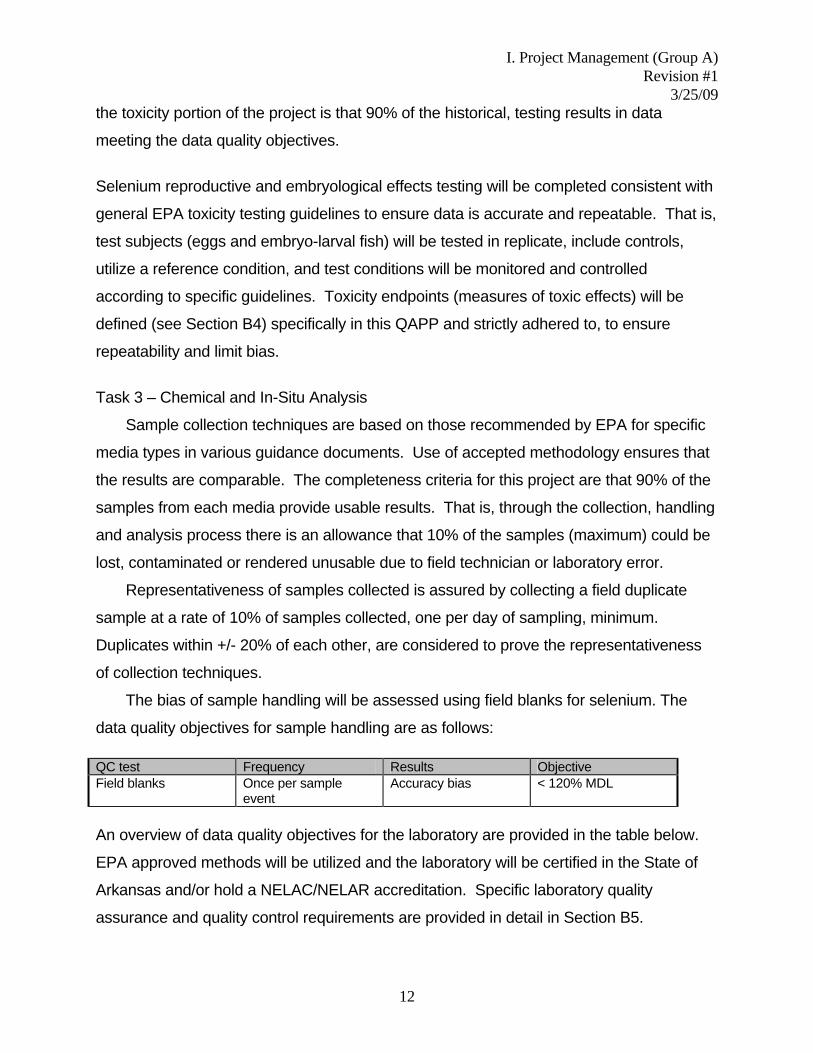
The bias of sample handling will be assessed using field blanks for selenium. The

data quality objectives for sample handling are as follows: QC test Frequency Results Objective Field blanks Once per sample

event Accuracy bias < 120% MDL

An overview of data quality objectives for the laboratory are provided in the table below.

EPA approved methods will be utilized and the laboratory will be certified in the State of

Arkansas and/or hold a NELAC/NELAR accreditation. Specific laboratory quality

assurance and quality control requirements are provided in detail in Section B5.

12


3/25/09 Sample Analysis Parameter Source/Method Units MDL Duplicate RPD Total Selenium EPA200.8 ug/l 1.0 ±20%* Dissolved Selenium EPA200.8 ug/l 1.0 ±20%* Fish Tissue Selenium EPA6020 mg/kg 0.1 ±20%* Total Alkalinity SM2320B mg/l 2.0 ±20% TDS SM2540C mg/l 1.0 ±20% TSS SM2540D mg/l 1.0 ±20% VSS EPA160.4 /

SM2540E mg/l 1.0 ±20%

Total Solids (Fish Tissue)

Sm2540G % 0.1 ±20%

Chlorophyll a SM10200H ug/l 2.0 ±15% *In the case of selenium the duplicates are matrix spike duplicates

13


3/25/09

A8 Special Training Requirements/Certification

All personnel participating in studies have been trained by experienced

scientists/engineers to complete the necessary tasks or are in the process of being

trained with appropriate oversight. Personnel participating in scientific studies shall be

familiar with the SOPs appropriate to that particular study and the QAP. Personnel

participating in scientific studies conducted pursuant to specific procedures specified by a

regulatory authority (e.g., a state or federal environmental agency) shall be familiar with

those specific procedures.

GBMc & Associates will oversee all sample collections, including collection of aquatic

biota. All field technicians will be trained for proper sample handling, preventative

maintenance, calibration and sample custody procedures. GBMc & Associates is

responsible for assuring that all field technicians are properly trained.

Great Lakes Environmental Center is responsible for toxicity testing and related

laboratory testing. All technicians are trained in the appropriate techniques and familiar

with the appropriate GLEC SOP’s. An SOP specific to the reproduction and embryo-

laurel terratogenicity test will be developed prior to initiation of the spring bioassessment.

This SOP will be site specific to the species of sunfish identified during early spring

reconnaissance.

AnaLab is responsible for chemical analysis of water, sediment and tissue samples.

All technicians are trained in the appropriate techniques and familiar with Analab SOP’s.

14


3/25/09

A9 Documentation and Records

A bound field logbook will be maintained documenting field activities during the

study. Log book entries shall include, dates of field activities, type of activities completed,

list of samples collected, and general observations pertinent to the study. Field data,

including sample collection and collection of aquatic biota will be recorded in a field log

book or on a field data sheet designed specifically for the field activity. Entries will include:

date and time of sample collection, name of person collecting samples, problems

encountered, and date and time of sample delivery. Logbooks and field data sheets will

be kept at the GBMc & Associates office except when in the field. Copies will be made of

all entries once per quarter.

All data collected during scientific studies should be checked by the team leader for

completeness and accuracy. Field data forms should be complete and initialed by the

completing scientist and the reviewing scientist.

Data entry to spreadsheets and databases along with spreadsheet calculations

shall be checked for accuracy at a rate of 10% (minimum) of the entries and calculation

cells. Copies of the checked data and spreadsheets should be initialed by the reviewer

and retained in the records.

All calculations should be detailed in the body of written reports, or shown on

GBMc & Associates Calculation Pages. Good notes regarding calculations should be

kept and filed in the project notebook.

All scientific reports shall be peer reviewed and/or reviewed by the Project

Manager prior to approval by a GBMc & Associates Principal.

Quality Assurance Assessment Reports will be prepared and submitted electronically

to the Project Manager at the mid point of the study and upon study completion. These

reports will document all QA problems and corrective actions, if any.

All laboratory data (from both toxicity testing and analytical analyses) shall be

reported quarterly, at a minimum, to GBMc & Associates in both hard copy and electronic

format. Data will be stored at GBMc & Associates for a minimum of 3 years.

15


3/25/09

The QAPP will be updated as necessary following an adaptive management protocol.

The Project Manager is responsible for providing updates to all of the parties listed in

element A3.

16

II. Data Generation and Acquisition (Group B) Revision #1

3/25/09

II. DATA GENERATION AND ACQUISITION (GROUP B) B1 Sampling Process Design The objective of the study is to complete a UAA of Loutre Creek and to develop a

SSC for Selenium based on the determined designated use and the historical water

quality. Figure 1 provides the locations of the sampling sites that will be utilized during the

study and Table B1.1 describes the stations. Field assessments and all sample collection

will be completed by GBMc & Associates field teams.

Table B1.1. Description of and Rationale for Project Sample Stations. Station I.D. Station Description

LC-0 Secondary background station on Loutre Creek, upstream of Outfall 001 and direct storm water influences from developed urban watershed.

LC-1 Background station on Loutre Creek, upstream of Outfall 001 and direct storm water influences from Lion Oil.

LC-3 Loutre Creek downstream of Outfall 001 in area of greatest effluent concentrations.

LC-4 Loutre Creek downstream of Outfall 001 and immediately upstream of confluence with Bayou De Loutre.

BDL-1 Background station on Bayou De Loutre, upstream of confluence with Loutre Creek but in potential land-use area affected by historical oil field uses.

BDL-2 Bayou De Loutre downstream of confluence with Loutre Creek.

Task 1 – Biological Assessment

A biological assessment (bioassessment) will be completed by GBMc & Associates at

each of the four sample stations to document the existing conditions of the streams

aquatic communities and physical habitat. Fish and macroinvertebrate collections will be

completed once during the spring season and once during the summer season to assess

the health of the aquatic community, maintenance of biological integrity and maintenance

of fishery uses. Detailed habitat assessment will be completed during each assessment

to document the available habitat, the existing condition of the channel and the condition

of the riparian corridor. Habitat data will be used to help discern if the aquatic community

15


3/25/09

is being impacted by habitat alone or also by water quality or combination thereof. Fish

will be collected using electro fishing techniques supplemented with seine hauls where

appropriate. Macroinvertebrates will be collected with kick nets using multi-habitat

protocols. All specimens will be identified to the lowest taxonomic level practicable.

Collections will be analyzed with several biometrics to determine community status.

Results of the assessment will be used to determine if Loutre Creek is maintaining an

perennial or seasonal fishery and if the biological integrity is impacted in such a way from

historical land uses that these uses are unattainable an warrant development of a sub-

category use. A summary of the experimental design is included in Table B1.2.



selenium on resident biota from Loutre Creek. The assessment will focus on reproductive

and embryological effects to fishes in the Centrachidae (sunfish) family. During the

spring/summer sampling season fertile females will be stripped and the eggs field

fertilized. Eggs will be sent to Great Lakes Environmental Centers laboratory for hatching

and development to a 96-hour stage. Eggs will be evaluated for fecundity and embryo-

larval stage fish will be evaluated for deformity to ascertain the potential impact of

selenium. Section B4 provides details of the testing protocol and the deformity

assessment. Selenium levels from the water column, eggs, fish tissue, sediment and

within primary producer (periphyton, phytoplankton, etc.) and primary consumer

(macroinvertebrates, fish, etc.) trophic levels will be measured at this time to develop a

relationship between water column levels and those affecting the test sunfish species.

That is, this relationship will be used to link total selenium levels in the water to levels that

cause impacts to fish reproduction in Loutre Creek. Samples from each media will be

collected at each sample station during the spring biological assessment event. Samples

of fish tissue, sediment and within primary producer and primary consumer trophic levels

will also be collected during the summer event. Sample size for fish tissue analysis will be

a minimum of four fish per station. A summary of the experimental design is included in

Table B1.2.

16


3/25/09


Various chemical parameters will be monitored during the study. During each of

two bioassessments and on four additional sample trips in-situ parameters will be

analyzed and samples collected for laboratory analysis from each sample station and

from Outfall 001. In-situ parameters shall consist of pH, temperature, dissolved oxygen,

specific conductance and turbidity. Water samples delivered to the laboratory will be

analyzed for total selenium, dissolved selenium, total alkalinity, total suspended solids,

total dissolved solids and volatile suspended solids. Samples from other media, if

collected, will be analyzed for total selenium. Additional parameters may be added as

necessary. In-Situ parameters will be measured by GBMc & Associates. Samples from

other media will be analyzed by AnaLab. Data from the chemical analysis will be utilized

to set-up and calibrate the fate and transport model. A summary of the experimental

design is included in Table B1.2.

Task 4 – Fate and Transport Modeling

A water quality model will be utilized to support the field data and further assess the fate

of selenium in the aquatic environment. The focus of the modeling will be to determine

the transport and deposition of selenium in the aquatic environment and to assess where

in the trophic structure the selenium is being deposited and/or taken up, and how much

bioaccumulation might be anticipated over time. Data for model initial conditions and

calibration will originate from the field data collected during this study. That is, upstream

measured water quality will serve as the background condition (or boundary condition) in

the modeling. The water quality inputs from Outfall 001 will serve as inputs to the system

and the downstream water quality will serve as targets for the calibration via coefficients

adjustments. In the case of the food chain model (trophic structure), data from each tier in

the food chain (producers, consumers, etc.) at each station, will serve as inputs and a

calibration guide for the modeling. Constants, coefficients and rates may be determined

from the field data collected, originate from the body of literature or be set by the

calibration process (but staying within the range of literature values).

17


3/25/09

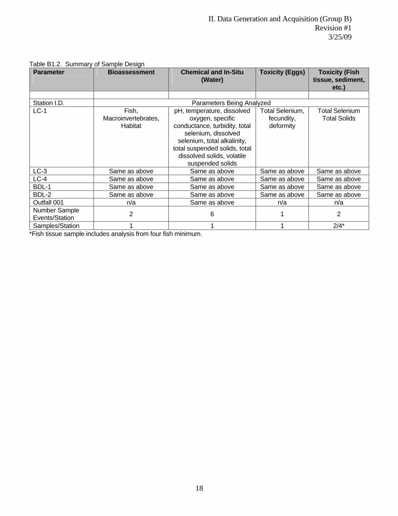
Table B1.2. Summary of Sample Design

Parameter

Bioassessment Chemical and In-Situ (Water)

Toxicity (Eggs) Toxicity (Fish tissue, sediment,

etc.) Station I.D. Parameters Being Analyzed LC-1 Fish,

Macroinvertebrates, Habitat

pH, temperature, dissolved oxygen, specific

conductance, turbidity, total selenium, dissolved

selenium, total alkalinity, total suspended solids, total

dissolved solids, volatile suspended solids

Total Selenium, fecundity, deformity

Total Selenium Total Solids

LC-3 Same as above Same as above Same as above Same as above LC-4 Same as above Same as above Same as above Same as above BDL-1 Same as above Same as above Same as above Same as above BDL-2 Same as above Same as above Same as above Same as above Outfall 001 n/a Same as above n/a n/a Number Sample Events/Station 2 6 1 2

Samples/Station 1 1 1 2/4* *Fish tissue sample includes analysis from four fish minimum.

18


3/25/09

B2 Sampling Methods Requirements The following section provides details of the sampling methodology and

procedures that will be utilized during the Loutre Creek UAA. Table B2.1 provides a

summary of sampling methodologies to be used during the study. GBMc & Associates

maintains a Quality Assurance Plan (QAP) for field data collection and data handling

(GBMc & Associates, 2008). Standard operating procedures (SOP’s) from the QAP

referenced in this section are provided in Appendix B.

Trained scientists will conduct the field sampling and other associated activities at

each sample location. Notes will be kept in field notebooks and/or specific field data

forms that record information collected during the study, unusual observations, and a log

of each day’s activities. All data forms, calibration logs, field notes, and other study

documentation will be reviewed by the Project Manager or Senior Scientist for

completeness and accuracy. Concerns over field data collection success or required

deviations to SOP will be reported to the project Quality Assurance Officer for review. Any

deviations to the methodologies described in this QAPP will be recorded and presented, in

detail (including an assessment of potential effect on data), in the final project report.

Task 1 – Biological Assessment

Bioassessments will be completed at each sample station to document the existing

conditions of the streams aquatic communities and physical habitat. Fish and

macroinvertebrate collections will be completed once during the spring season and once

during the summer season and detailed habitat assessment will be completed during

each bioassessment. Habitat assessment protocols will follow the SOP for Semi-

Quantitative Habitat Assessment as described in the GBMc & Associates Quality

Assurance Plan (QAP). The habitat assessment will cover an area of stream (the reach)

equal to a distance of at least 20X the average bankfull width. A two man field team will

complete the assessment. Data collected during the habitat assessment includes

qualitative (dominant substrate, bank stability, canopy density, etc) and quantitative

(thalwag depth, bankful depth and width, velocity, flow, etc) measures. Flow

19


3/25/09

measurements will be made at each station as part of the habitat assessment. Flow will

be measured using a velocity meter and wading rod and following GBMc SOP. Flow will

be calculated according to the velocity area method. Habitat data will be used to help

discern if the aquatic community is being impacted by habitat alone or also by water

quality.

Fish will be collected within the defined habitat reach using electro fishing

techniques supplemented with seine hauls where appropriate. Fish collection procedures

will follow the GBMc SOP as found in their QAP (GBMc & Associates, 2008). Collected

fish will be placed in a 5-gallon style bucket prior to analysis. After cursory field

identification and enumeration large healthy specimens are returned to the stream and

recorded as “released” in the log book and on the field record sheet. The remainder of

the collection is preserved in formalin for transport to GBMc & Associates. Fish will be

positively identified by trained taxonomists at GBMc & Associates. Each assemblage

collected will be evaluated with several biometrics to determine health of the community

and maintenance of biological integrity. Comparisons will be made between stations to

determine the maintenance of the fishery use downstream of Outfall001.

Macroinvertebtrate collections will be completed within the defined habitat reach

using a kick net in multiple habitats (multi-habitat consisting of rootwads, emergent

vegetation, undercut banks, deposition, etc.) found in the pool dominated stream system.

The method utilized is generally based on the Rapid Bioassessment (RBA) Protocols of

the USEPA (Barbour, 1999) where a dip net is utilized to sample a defined area of aquatic

habitat (typically 3m2) or for a defined time period (typically 3 minutes) in each sample

reach. Material from each bucket is condensed and field sorted or, preserved and

transported to the lab for sorting and enumeration. A grid and sorting tray (Caton style) is

used to randomly select sub-samples of the collected material for picking (organism

removal). Each randomly selected grid was picked until all organisms were removed.

Following protocol, when the number of picked organisms exceeds 90 (100 ± 10%) the

sub-sample is considered complete. If the number of organisms is less than 90, another

grid is randomly selected and all organisms are removed. This process continues until the

number of organisms exceeds 90. All organisms are preserved in 70% ethanol and

identified to the lowest practicable taxonomic level, generally to genus. Further detail on

20


3/25/09

these protocols can be found in the GBMc QAP. Collections will be analyzed with several

biometrics to determine community status.



selenium on resident biota from Loutre Creek. Samples from each media (water column,

eggs, fish tissue, sediment and within primary producer (periphyton, phytoplankton, etc.)

and primary consumer (macroinvertebrates, fish, etc.) trophic levels) will be collected at

each sample station during the spring biological assessment event and analyzed for

selenium and other constituents (see Task 3 below). Samples of fish tissue, sediment

and primary producer and primary consumer trophic levels will also be collected during

the summer event. Sample size for fish tissue analysis will be a minimum of four fish per

station. The assessment will focus on reproductive and embryological effects to fishes in

the Centrachidae (sunfish) family. During the spring sampling season fertile females will

be captured, striped and the eggs field fertilized. Eggs will be assessed and hatched by

Great Lakes Environmental Centers laboratory. Eggs will be incubated, monitored

individually and fecundity recorded. Once hatched the fish will be raised to an age of 5-

days and evaluated for deformity using a deformity index (GSI, etc.) Details on the

deformity index are provided in Section B4. This process will be completed for each of the

sample stations, including the LC-1 station which will serve as a baseline for fecundity and

deformity. Specific details of the sampling for the toxicity assessment are provided below.

A. Source of test organisms - Eggs from a sunfish species will be collected from each

monitoring station. Eggs will be collected from 5 to 10 fish from each site (same

species for all sites).

B. Collection of eggs - Eggs will be fertilized in the field using milt from males

collected from the same site. Eggs will be hand-expressed from the females. Milt

will be hand expressed or gonads will be simply removed from 2 to 3 ripe males

and then composited. Each batch of eggs will be fertilized with one to two ml of

sperm and gently mixed. Dead and/or broken eggs will be removed. Fertilized

eggs will be water-harden for 1 to 2 hours. The water-hardened eggs will be

21


3/25/09

transported to an on-site or local laboratory in O2-saturated laboratory or reference

water.

C. Tissue analysis - After removing the eggs, female lengths and weights will be

measured. Selenium will be measured in the each female from which eggs were

collected (muscle and whole body) and in a sub-sample of each batch of eggs.

Tissue samples will be kept frozen prior to analysis.


Various chemical parameters will be monitored during the study. During each of six

sample events in-situ parameters will be analyzed and samples collected for laboratory

analysis from each sample station and from Outfall 001. In-situ parameters shall consist

of pH, temperature, dissolved oxygen, specific conductance and turbidity. In-Situ

parameters will be measured at the time of sample collection using a portable field

meter(s). Field meters will be calibrated following the SOP from the GBMc & Associates

QAP which generally adheres to manufacturer’s recommendations.

Water samples will be collected as grab samples from the main flow area in the

channel. Water samples delivered to the laboratory will be analyzed for total selenium,

dissolved selenium, total alkalinity, total suspended solids, total dissolved solids and

volatile suspended solids. Sediment samples will be collected with clean stainless steel

sample apparatus (spoons, corers, etc.) and placed in clean containers for shipment to

the laboratory. Samples from other media will be collected following similar protocols

using clean containers. Samples from all media will be analyzed for total selenium.

Additional parameters may be added as necessary. In-Situ parameters will be measured

by GBMc & Associates. Samples from other media will be analyzed by AnaLab. Data

from the chemical analysis will be utilized to set-up and calibrate the fate and transport

model.

Samples will be analyzed in the laboratory according to the procedures outlined in

the most current release of Standard Methods for the Examination of Water and

Wastewater. Where specific EPA approved analysis methods exist the laboratory shall

use them. Table B2.2 summarizes the samples taken, the analytical method, the

preservative, and the holding time. A laboratory certified in the state of Arkansas shall

22


3/25/09

conduct all chemical analyses. AnaLab will serve as the laboratory of record for the

analytical analyses.

Table B2.1. Summary of Sampling Methods Sample Type GBMc

QAP SOP Number

Sampling Equipment

Field Processing Protocol

Storage Vessel

Preservative Designated Record Sheet (Y / N)

Fish SOP 10.0 Electro Shocker, Seines

Sort, Cursry ID and Tally, Preserve, Label, Store

Large PE Bottles/Buckets

Formalin Y

Macroinvertebrates

SOP 9.0 Aquatic Dip Net Condense, Qualitative Tallies, Preserve, Store

Large PE Bottles/Buckets

70% Ethanol or Kaylee’s

Y

Habitat SOP 7.0, 5.0

Wading Rod, Tape Measure, Flow Meter

n/a n/a n/a Y

Water SOP 12.0 Sample Bottles Label and Store in Ice Chest

Various Bottles (see Table ##)

Various (see Table ##)

Y

In-Situ SOP 1.0, 2.0, 3.0, 4.0, 14.0

Field Meters Calibrate, Measure in Main Channel

n/a n/a Y

Sediment n/a Stainless Steel Spoons, Corer

Label and Store in Ice Chest

Wide Mouth Glass Jars

4° C Y

Eggs n/a Gloves, Glass Containers, Mixing Containers


Plastic Widemouth Bottles

None Y

Fish Tissue SOP 17.0 Knives, Calibrated Scales, process Composite


Decon. Aluminum Foil, Foil/Brown Pot Plastic Bags

4° C Y

Biomass (whole body/cell)

SOP 15.0, 16.0

Periphytometer, Dip Nets, Sample Bottles


PE Bottles or Whirl Paks

4° C N

23


3/25/09

Table B2.2. Summary of water samples taken for analytical analysis for each monitoring event.

Parameter Number Samples/Event

Analytical Method Preservative Holding Time

Total Selenium 6 EPA200.8 HNO3, 4° C 180 Days Dissolved Selenium 6 EPA200.8 HNO3, 4° C 180 Days Total Alkalinity 6 SM2320B 4° C 14 Days TDS 6 SM2540C 4° C 4 Days TSS 6 SM2540D 4° C 7 Days VSS 6 EPA160.4 / SM2540E 4° C 7 Days Chlorophyll a 6 SM10200H Frozen 21 Days1

SM = Standard Methods for the Examination of Water and Wastewater. 1 Filtered and frozen in field prior to shipment to extend holding time.

24


3/25/09

B3 Sample Handling and Custody Requirements All samples will be placed in the appropriate clean containers supplied by the

laboratory. Each sample container will be labeled with the sample I.D., date, time, and

initials of collector(s). Samples will be placed in ice chests and maintained at 4º C for

delivery to the laboratory in a timely manner conducive to maintenance of regulatory

holding times. Samples collected for chlorophyll-a analysis will be filtered and frozen prior

to shipping to prolong the holding time to 21 days. Chain of Custody (COC) forms that

include information on each sample delivered to the laboratory for analysis will be

completed. Each COC form will be signed by each person handling the samples from

collection in the field to receipt in the laboratory. The COC form will include all required

information and will be checked for completeness prior to submission of samples to the

laboratory.

.

25


3/25/09

B4 Analytical Methods Requirements Chemical Analysis

All procedures used for analyzing chemical parameters of water quality for

reporting purposes will follow USEPA approved methods and/or Standard Methods for the

Examination of Water and Wastewater (latest edition).

Analytical methods are listed below, along with specific performance requirements.

All analytical analyses will be completed by a laboratory certified in the State of Arkansas.

All analytical methods will be conducted under the AnaLab Quality Assurance Plan in

which there is a specific SOP for each method (Appendix C). All methods fall under the

specific quality control requirements outlined in the Quality Assurance Plan. Any failure in

the analytical systems will be the responsibility of AnaLab to apply necessary corrective

action.

Failures in the QA system encountered by AnaLab shall be reported to the project

Quality Assurance Officer (QAO) as soon as reasonably possible.

Table B4.1. Summary of analytical methods. Parameter Source/Method Units MDL Total Selenium EPA200.8 ug/l 1.0 Dissolved Selenium

EPA200.8 ug/l 1.0

Fish Tissue EPA6020 Mg/kg 0.1 Total Alkalinity SM2320B mg/l 2.0 TDS SM2540C mg/l 1.0 TSS SM2540D mg/l 1.0 VSS EPA160.4 / SM2540E mg/l 1.0 Total Solids SM2540G % 0.1 Chlorophyll a SM10200H ug/l 2.0

Toxicity Assessment

The toxicity assessment task is focused on the reproductive and embryo-larval effect. A

description is provided below.

Reproductive and embryo-larval effect assessment

26


3/25/09

Fertilized eggs will be monitored in a Great Lakes Environmental Center laboratory or on-

site laboratory for:

• Percent hatch

• Larval survival (to swim-up stage, 5 days post hatch)

• Embryo-larval malformations, including

o Edema

o Skeletal deformities (lordosis, kephosis, and scoliosis)

o Craniofacial deformities (head, eyes, or jaw)

o Fin deformities

o Embryo-larval malformations will be graded using a scoring system

termed graduated severity index (GSI)

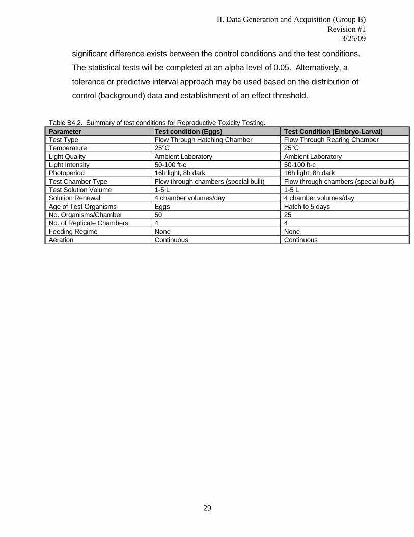
A detailed description for the toxicity assessment is provided below. Table B4.2 provides

a summary of the test conditions.

A. Egg and Larvae Rearing for Effects Assessment – Sub-samples from each batch

of eggs will be assessed for percent hatch/larval survival and malformations.

B. Percent hatch and larval survival - From a given batch of eggs, 200 fertilized eggs

will be divided into 4 replicate hatching jars (50 eggs/jar). Hatching jars will have a

screen (e.g., 35 mesh) on the bottom. Hatching jars will be submerged in a

temperature controlled aquaria containing reference water. A rocker arm will

continuously move the jars up and down in the aquaria to maintain movement of

fresh water across the eggs. The reference water in the aquaria will be aerated

and replaced at a rate of at least 4 tank turnovers per day via a flow through

system. The number of hatched larvae will be monitored daily.

From each hatching jar, 25 newly hatched larvae will be transferred to a separate

beaker with a screen on the bottom for the 5-day larval survival assessment; i.e.,

for each batch of eggs there will be 4 replicate larval survival beakers containing 25

larvae each. Each survival beaker will be suspended in a temperature controlled

27


3/25/09

flow-through aquarium containing well aerated reference (synthetic) water. Survival

will be monitored daily through the swim-up stage, 5 days post hatch.

C. Malformations (deformity) assessment - From a give batch of eggs, 500 fertilized

eggs will be placed into a hatching jar for the assessment of embryo-larval

malformations. The bottom of each hatching jar will be a screen (35 mesh). The

hatching jar will submerged in an aquarium and fitted to a rocker arm similar to that

described above. At the completion of yolk sac absorption, larvae will be sacrificed

with MS-222 (0.8 g/L) and preserved in Davidson’s solution.

All hatched larvae after yolk absorption will be assessed for the frequency and

severity of skeletal (lordosis, kephosis, and scoliosis), craniofacial (head, eyes, or

jaw) and fin deformities as well as edema. For each deformity type, the number of

deformed progeny from a single adult will be summed and divided by the total

number of larvae assessed from that adult (×100) to obtain a mean percentage of

deformities. Each fish will be scored on the basis of the severity of each type of

deformity on a scale from 0 (normal) to 3 (severely deformed). Photographs of the

deformities and associated scores will be taken and used in the grading of the

graduated severity index (GSI). In general, scoring of the deformities will be: 0 =

normal, 1 = slight defect of size or structure, 2 = moderate defect of size or

structure, and 3 = severe defect of size or structure. The sum of the individual

scores for each larva will be calculated for each of the four malformations (edema,

skeletal, craniofacial and fin deformities) and a GSI score will be determined for

female/batch of eggs. At least 10% of the scores made by the primary analyst will

be confirmed by a separate analyst to confirm consistency in scoring. If there is

greater than a 20% difference in scoring, samples will be reanalyzed after

consultation with the analysts and review of the criteria for scoring provided with the

photographs.

A statistical procedure consistent with those used for routine toxicity testing

(ANOVA, Bonferroni test, Kruskal-Wallis test, etc.) will be used to determine if a

28


3/25/09

significant difference exists between the control conditions and the test conditions.

The statistical tests will be completed at an alpha level of 0.05. Alternatively, a

tolerance or predictive interval approach may be used based on the distribution of

control (background) data and establishment of an effect threshold.

Table B4.2. Summary of test conditions for Reproductive Toxicity Testing. Parameter Test condition (Eggs) Test Condition (Embryo-Larval) Test Type Flow Through Hatching Chamber Flow Through Rearing Chamber Temperature 25°C 25°C Light Quality Ambient Laboratory Ambient Laboratory Light Intensity 50-100 ft-c 50-100 ft-c Photoperiod 16h light, 8h dark 16h light, 8h dark Test Chamber Type Flow through chambers (special built) Flow through chambers (special built) Test Solution Volume 1-5 L 1-5 L Solution Renewal 4 chamber volumes/day 4 chamber volumes/day Age of Test Organisms Eggs Hatch to 5 days No. Organisms/Chamber 50 25 No. of Replicate Chambers 4 4 Feeding Regime None None Aeration Continuous Continuous

29


3/25/09

B5 Quality Control Requirements Field Sampling

Duplicate samples for key constituents (Total Selenium, TSS, and VSS) shall be

collected at a minimum frequency of 10% of the samples collected for the entire study. At

least one duplicate sample will be collected for each day of sampling. Duplicate samples

shall vary by no more than 20% relative percent difference (RPD) or the sample results

will be considered suspect. In the event an RPD exceeds 20%, the Project QAO will

investigate the incident to determine the cause of the exceedance and what action, if any,

is necessary.

One field blank will be collected during each sample event for analysis of total

selenium. Field blanks will consist of a sample of ultra pure laboratory water poured into

the appropriate sample container in the field to simulate all possible contaminant

exposures. Sampling methodology and equipment must be the same for field blanks as

for routine sampling in the study. If a field blank is found to be contaminated, by a

chemical of concern, an analysis will be conducted to determine the potential impact of

the contamination on the results of the associated batch of samples. The Project QAO

will determine the appropriate course of action from the results of the analysis.

Analytical Laboratory

The laboratory will validate analytical data by use of blanks, laboratory controls,

spikes, and spike duplicates. Laboratory blanks measure the amount of each respective

analyte contributed from the analytical procedure. A laboratory blank is considered out of

control for a specific analyte if the value exceeds the higher of either the minimum

detection limit (MDL) or 5% of the measured concentration in the sample. A laboratory

control measures the ability of the laboratory to recover an analyte from a blank matrix.

The laboratory spike sample is used to evaluate the laboratory’s ability to recover an

analyte in the sample matrix. The QC exceedence criteria for laboratory controls and

spikes is based on upper and lower control limits derived from the laboratory’s method

specialized limits. The laboratory spike duplicate is used to evaluate the laboratory’s

precision (ability to attain similar analytical results from duplicate samples). A RPD is

30


3/25/09

calculated for the spike and spike duplicate. The RPD is compared to method specialized

limits to determine QC exceedance. Any significant excursion from one of the QC

parameters will result in a repeat of the analysis in question following an investigation by

the laboratory as to the cause of the QC excursion and a report of the corrective actions

taken to the project QAO.

Specific laboratory quality control requirements for each analytical method is listed

for each parameter in the table below.

Table B5.1. Summary of laboratory QA requirements.

Parameter Source/Method Duplicate RPD (%)

LCS Recovery

(%)

LCS RPD (%)

Matrix Spike

Recovery (%)

Matrix Spike RPD (%)

Total Selenium EPA200.8 n/a 85-115 20 70-130 20 Dissolved Selenium

EPA200.8 n/a n/a n/a 70-130 20

Fish Tissue Selenium

EPA6020 n/a 85-115 20 70-113 20

Total Alkalinity SM2320B 20 n/a n/a 10 n/a TDS SM2540C 20 15 n/a n/a n/a TSS SM2540D 20 10 n/a n/a n/a VSS EPA160.4/SM2540E 20 n/a n/a n/a n/a Total Solids (fish tissue)

SM2540G 20 n/a n/a n/a n/a

Chlorophyll a SM10200H 15 15 n/a n/a n/a Toxicological Laboratory Great Lakes Environmental Center will validate toxicity data through use of a reference

site condition and laboratory controls. Eggs from fish collected from a reference site will

be carried through the testing process to serve as a baseline for selenium effects.

Laboratory controls demonstrate that the test organisms used are healthy and able to

produce reasonable results. Potential variability in the malformation assessment phase

will be controlled by regular audits of the scores and by duplication of scoring on selected

batches at a rate of 10%.

31


3/25/09

B6 Instrument/Equipment Testing, Inspection, and Maintenance Requirements

Equipment cleaning and maintenance procedures will follow manufacturer

recommendations. Records of maintenance of field sampling equipment will be kept in a

record book listing name of technician, date and type of maintenance. Portable field

meters should be calibrated in the lab at least twice/month (every other week) to monitor

readiness and ensure proper functionality. Each day during a field trip equipment should

be inspected before use (during calibration, etc.) to ensure functionality. All equipment will

be inspected and cleaned immediately following a field trip and stored in a safe place to

allow its future readiness.

Where appropriate, calibration and performance tests are described in the SOP of

the respective application. Generally, all equipment will be utilized per the manufacturer’s

directions. If during the course of the field activities equipment fails to conform to known

QA/QC requirements, the equipment will be repaired or replaced with similar equipment

that will meet QA/QC requirements.

32


3/25/09

B7 Instrument Calibration and Frequency Field meters will be calibrated prior to each sampling event. DO Probes will be

corrected for barometric pressure and calibrated to 100% saturation. Ph probes will be

calibrated using a pH 4 and a pH 7 calibration solution. Turbidity meter readings will be

checked against standards, if more than 20% off the known value the meter will be

calibrated following the SOP. Specific conductance will be checked against known

standards, if more than 20% off the known value the meter will be calibrated following the

SOP. All meter calibrations will be completed following GBMc SOP’s which are provided

in Appendix B of this document.

.

33


3/25/09

B8 Inspection/Acceptance Requirements for Supplies and Consumables

Supplies and consumables used for this project will include sample bottles,

preservative, toxicity sample materials, laboratory reagents necessary for the tests

performed and calibration standards. All sample bottles will be new clean bottles of a

style and material consistent with analytical requirements. All consumables will be

purchased new. All lab supplies and consumables will be approved by the Project

Manager or the Lab Manager (in the case of analytical or toxicity testing). All chemicals

and reagents will be dated and inspected for proper expiration date when purchased and

prior to use. All supplies will be inspected when purchased and any damaged or open

containers or packaging will be refused.

34


3/25/09

B9 Non-Direct Measurements Existing data from past studies and from the existing literature will be used in

portions of this study. The table below outlines the data that will be used, where it will be

used in the study and the acceptance criteria for its use.

Table B9.1. Summary of use of non-direct data (existing) data in the study. Data Description Use in Study Acceptance Criteria Selenium data from recent studies. Media include water, sediment and fish tissue.

Support for toxicity testing, modeling and SSC development.

Meets same rigors as that outlined in this QAPP.

Routine WET Test as required by the NPDES permit.

Support for toxicity testing and SSC development.

Meets NPDES program requirements for reporting on DMR’s.

Scientific studies from the body of literature dealing with Selenium toxicity and bioaccumulation

Support in toxicity testing and SSC development.

Only peer reviewed scientific literature or published test books will be considered.

Scientific literature for modeling rates, constants and coefficients.

Aid in development of modeling rates, constants and coefficients for prediction of selenium fate and transport in the aquatic environment.

Only peer reviewed scientific literature or published test books will be considered. Focus will be given to EPA guidance documents.

Scientific literature concerning selenium treatability.

Support alternatives analysis. Only peer reviewed scientific literature or published test books will be considered.

35


3/25/09

B10 Data Management

Upon conclusion of all activities at a given study location, the QAPP/study plan

should be reviewed to ensure all necessary data was collected. The field team should

review all completed data forms and sample labels for accuracy, completeness, and

legibility, and make a final inspection of samples. If information is missing from the forms

or labels, the team leader should fill in the missing information prior to proceeding to the

next study location. Any missing and/or compromised samples should be collected

immediately. A field notebook should be maintained by the field team leader (at a

minimum) to document field activities, data collected, deviations from method, and

general observations and information related to the study. Every person should maintain

individual field logs to document activities and observations during daily activities.

All data collected during scientific studies should be checked by the team leader for

completeness and accuracy. Field data forms should be complete and initialed by the

completing scientist and the reviewing scientist. All field data sheets and log books will be

kept at GBMc and maintained for a period of 5 years.

All field data will be entered to spreadsheets (or databases) or scanned into pdf

files for electronic storage. Data will be stored electronically in project files on a secure

network. The network is backed up weekly onto magnetic tape media. Data entry to

spreadsheets and databases along with spreadsheet calculations shall be checked for

accuracy at a rate of 10% (minimum) of the entries and calculation cells. Copies of the

checked data and spreadsheets should be initialed by the reviewer and retained in the

records. All calculations should be detailed in the body of written reports, or shown on

GBMc & Associates Calculation Pages. Good notes regarding calculations will be kept

and filed in the project notebook.

GBMc & Associates is responsible for the compilation of all data (in-situ,

bioassessment, analytical, toxicity, etc.) collected during the study. Analytical and toxicity

results as well as QA/QC results will be reported in electronic format to the Project

Manager once per quarter, at a minimum. This data will be stored on the GBMc &

Associates network for a minimum of fine years after the end of the project.

36


3/25/09

All deliverables (scientific reports, QA/QC reports, etc.) developed as part of this study

shall be peer reviewed and/or reviewed by the Project Manager prior to being sent to Lion

Oil, ADEQ or EPA.

37

III. Assessment and Oversight (Group C) Revision #1

3/25/09

III. ASSESSMENT AND OVERSIGHT C1 Assessments and Response Actions Data will be reviewed by the GBMc QA Officer to evaluate the QAPP and its

implementation. The review will include the following objectives:

a) collection of samples

b) corrective actions

Laboratory performance may be checked using external audit samples. GBMc QA

Officer will be the internal individual responsible for detecting any errors or malfunctions

and performing corrective actions. If errors are detected or anomalous data is suspected,

the data will be traced back through the acquisition process until the error is found. In the

advent that no error is found the data will be considered appropriate for reporting. If an

error is found and cannot be resolved, then the effected data will be discarded.

Regulatory reviews by ADEQ and EPA of the draft and final documents will

facilitate adherence to the QAPP.

38

III. Assessment and Oversight (Group C) Revision #1

3/25/09

C2 Reports to Management Quarterly progress reports will be made to the Project Manager by Great Lakes

Environmental Center (GLEC) and Ana-Lab detailing significant occurrences related to

the project including number of samples taken, surveys completed operational problems

and corrective actions. Quarterly Quality Assurance reports will be made to the QAO and

the Project Manager by the Field Coordinator, GLEC and Ana-Lab detailing all QA

problems and corrective actions. Copies of all reports will be maintained at the GBMc &

Associates office for a period of five years.

As required by the CAO Lis No 08-104, quarterly reports relating schedule

compliance will be submitted to ADEQ NPDES Enforcement Section.

39

IV. Data Validation and Useability (Group D) Revision #1

3/25/09

IV. DATA VALIDATION AND USABILITY D1 Data Review, Validation, and Verification

Requirements Chemical results will be rejected if they fall outside of the standard deviation for the

respective parameter as outlined in Section A7. The review, validation and verification of

the analytical data are the responsibility of Ana-Lab. The review, validation and

verification of the toxicological data are the responsibility of GLEC.

The review, validation and verification of field data and lab results for reporting are

the responsibility of GBMc & Associates.

40


3/25/09

D2 Validation and Verification Methods The field and lab data will be combined in the spreadsheets and reported to the

Project Manager once per quarter at a minimum. GBMc & Associates will validate and

verify the data in the reports to be correct by checking all entries against lab results and

field notebook entries.

41


3/25/09

D3 Reconciliation with Data Quality Objectives Laboratory data quality objectives and their fulfillment will be assessed immediately

after the analyses are performed. Data found to be outside objectives will be reanalyzed

immediately if possible and discarded if not. Laboratory objectives and assessment in

element B5.

Sample handling data quality objectives will be assessed by analysis of field

blanks. Sample handling quality objectives will be assessed quarterly, at a minimum once

per year and reported in the final report.

Sampling data quality objectives will be met by designing the sampling protocol so

that the error involved in sampling is equal to or less than the prescribed objective. They

will be assessed by analysis of field duplicates. They should agree with each other within

20 percent.

Any deviations from the objectives will be reported to the GBMc QAO quarterly and

attempts will be made to determine and fix the causes of the data not meeting objectives.

42

Appendix A Selenium Data from Lion Oil Company Outfall 001

Appendix B GBMc SOP

c

1.0 pH Meter Calibration SOP Purpose This SOP describes the methods for calibration and use of portable pH meters (capable of 2-point calibration) such as the Orion® Star Series pH meter and YSI Multi Probe System (MPS). Field forms used for meter calibration and measurement recording are attached to this SOP. Procedure Orion® Star Series (or similar pH meter) Calibration 1. Be sure that the electrode (probe) is properly attached and that a good battery is

installed. 2. Turn the meter on and check the read-out for any warning messages (“Low Bat.”,

etc.) If problems occur refer to the owners manual for help. 3. Record the proper information (date, time, etc.) on the Calibration Field Form

(attached) or in a field logbook. 4. Remove the probe protection cap, rinse and place the probe in pH buffer solution

7.00 (yellow in color) submerging the end to at least 1 inch. Allow the meter to adjust to the buffers pH for approximately 1 minute.

5. Press the Calibration button on the meter to begin the calibration process. The

display should read “CAL.1” along with the pH reading. 6. When the meter has accepted the buffer the pH will stop flashing. Press the

Calibration button to accept the value and proceed to the next calibration point “CAL.2”

7. Remove the probe from the 7.00 buffer and rinse with distilled water to remove any

excess buffer solution. 8. Place the probe in the second buffer solution, 4.01 (pink) or 10.01 (blue),

whichever best brackets the expected pH range to be measured, and stir it gently.

GBM v1.2 January 2008 Page 1 of 5

c

9. When the meter has accepted the value the pH will stop flashing as in step 6 above. Press “Save” to accept this value. Record this number on the pH Calibration Record sheet.

10. The display will immediately show the slope, a number that should be between

92% and 102%. Record this number on the pH Calibration Record sheet. If the slope is larger or smaller than this range the meter should be recalibrated.

11. A calibration check should be done once the meter is calibrated. This is done by

rinsing the probe with distilled water and then placing it in the pH 7.00 buffer solution and taking a reading. Make sure the measure symbol is lit, if not press the “Measure” button to return to measurement mode. When the pH stops flashing record this reading on the pH Calibration Record form. If the reading is between 6.90 and 7.10 then the original calibration remains valid. If the measurement falls outside this range then the meter should be recalibrated.

12. Gently shake or rinse off excess liquid from the probe. The meter is now ready for

use. 13. The pH meter should be calibrated once per day on days that it is used. The pH

meter should have its calibration checked once for each sampling trip or once every 10 samples whichever is greater. This is done simply by placing the probe in the pH 7.00 buffer solution and taking a reading. Record this reading on the pH Calibration Record form. If the reading is between 6.90 and 7.10 then the original calibration remains valid. If the measurement falls outside this range then the meter should be recalibrated. Furthermore, if the battery or probe is ever disconnected from the meter during use, a new calibration would be required.

YSI MPS 1. Be sure that the pH electrode (probe) is properly attached and that a good battery

is installed.

2. Turn the meter on and check the read-out for any warning messages (“Low Bat.”, etc.) If problems occur refer to the owners manual for help.

3. Record the proper information (date, time, etc.) on the Calibration Field Form

(attached) or in a field logbook. 4. Press the On/off key to display the run screen then press the Escape key to

display the Main Menu screen.

5. Use the arrow key to highlight the Calibrate selection and press Enter.


c

6. Use the arrow keys to highlight the pH selection and press Enter to display the pH calibration screen.

7. Select the 2-point option to calibrate the pH sensor using two calibration standards

then press Enter. The pH Entry Screen is displayed.

8. Remove the transport/calibration cup from the end of the probe and place the probe in pH buffer solution 7.00 (yellow in color) so that the sensor is completely immersed, approximately 30 mL.

9. Screw the transport/calibration cup on the threaded end until securely tightened.

Gently rotate and/or move probe module up and down to remove any bubbles from the pH sensor.

10. Use the keypad to enter the calibration value of the buffer being used and press

Enter. The pH calibration screen is displayed. Allow at least one minute for temperature equilibration before proceeding.

11. Observe the reading under pH, when the reading shows no significant change for

approximately 30 seconds, press Enter. The screen will indicate that the calibration has been accepted and prompt you to press Enter to Continue.

12. Press Enter. This returns you to the Specified pH Entry Screen. Rinse the probe

module, transport/calibration cup and sensors in distilled water. 13. Repeat steps 8 through 11 using the second pH buffer solution, 4.01 (pink) or

10.01 (blue), whichever best brackets the expected pH range to be measured. 14. Press Escape to return to Main Menu. Use the keypad and select Run. 15. A calibration check should be done once the meter is calibrated. This is done

simply by placing the probe in the pH 7.00 buffer solution and taking a reading. Record this reading on the pH Calibration Record form. If the reading is between 6.90 and 7.10 then the original calibration remains valid. If the measurement falls outside this range then the meter should be recalibrated.

16. Gently shake or rinse off excess liquid from the probe. The meter is now ready for

use.

17. The pH meter should be calibrated once per day on days that it is used. The pH meter should have its calibration checked once for each sampling trip or once every 10 samples whichever is greater. This is done simply by placing the probe in the pH 7.00 buffer solution and taking a reading. Record this reading on the pH Calibration Record form. If the reading is between 6.90 and 7.10 then the original calibration remains valid. If the measurement falls outside this range then the


c

meter should be recalibrated. Furthermore, if the battery or probe is ever disconnected from the meter during use, a new calibration would be required.

pH Measurements Orion® Star Series (or similar pH meter) 1. Place the probe in the liquid to be analyzed and stir it gently. The probe should be

submerged so that the sensor is at least 1 inch into the liquid. 2. Press the “Measure” button to begin. The measure symbol will flash until the

reading is stable. When the pH stops flashing record the reading to the nearest tenth of a unit.

3. Be sure to turn off the meter when the final pH measurement has been taken and

recorded. YSI MPS 1. Select Run from the main menu to display run screen.

2. With probe sensor guard installed, completely immerse all sensors into sample.

3. Allow the meter to stabilize and record the pH reading to the nearest tenth of a unit.

Meter Maintenance/Storage Orion® Star Series (or similar pH meter) 1. Store the meter in a safe dry place. 2. Keep the probe cover on the probe when not in use and between measurements. 3. A small piece of sponge or paper towel soaked in pH buffer 7.00 should be placed

in the bottom of the probe cover to keep the probe surface wetted with the buffer. The probe should never be allowed to dry out.

4. Use only “Low Maintenance Triode” ATC probes with the Star series pH meters

(model # 9107BNMD or equivalent.)


c

YSI MPS 1. Store the meter in a safe dry place. 2. Keep a moist sponge in the transport/calibration cup and keep sealed when not in

use and between measurements. The probes should never be allowed to dry out. Quality Assurance/Quality Control 1. Meters are calibrated biweekly (at a minimum) to ensure proper function and

accuracy. 2. Values measured during biweekly calibrations are compared between meters to

verify accuracy. 3. Duplicate measurements should be taken at a rate of 10% (minimum) of samples

analyzed.


2.0 Dissolved Oxygen (D.O.) Meter Calibration SOP Purpose

This SOP describes the methods for calibration and use of the portable YSI Model 58 and Model 85 D.O. meters as well as the YSI MPS. Field forms used for meter calibration and measurement recording are attached to this SOP.

Procedure

Calibration

Model 58 1. Be sure that the oxygen probe is properly attached to the meter and that the end of

the probe is affixed in storage bottle containing a piece of wet sponge or towel to keep the probe moist, and to provide a water-saturated air environment.

2. Turn the meter on and check the read-out for the “LOBAT” warning, and for the

normally observed display readings. If problems occur refer to the owners manual for help.

3. Record the proper information (date, time, etc.) on the Dissolved Oxygen

Calibration Record sheet or in a field logbook. 4. Set the D.O. meter to “ZERO” and use the “O2 ZERO” knob to adjust the display to

0.0. If the meter will not adjust to zero refer to the owners manual for guidance. 5. Perform a Calibration according to one of the following procedures:

Winkler Titration (verification calibration) a) Fill a container with at least 500 mL distilled water (or tap water if distilled not

available) and allow it to acclimate. It can be aerated overnight to achieve 100% oxygen saturation if desired.

b) Fill each of two BOD bottles with the water from the container by gently submerging them into the container.

c) Add one each of the HACH manganous sulfate and alkaline iodide-azide powder pillows to each bottle. Cap the bottles and invert them 15-20 times to mix the solution thoroughly.

d) Allow the bottles to settle until a precipitate appears in the bottom half of the bottle. This will usually take 3-5 minutes.

e) Add one HACH sulfamic acid powder pillow to each BOD bottle. Invert the bottles until all the precipitate has been dissolved.


c

f) Using a graduated cylinder measure and place 200 mL of the solution into a

flask. g) Add 1 mL of HACH starch indicator to the flask. The solution should turn

black. h) Using a burette filled with sodium thiosulfate (at room temperature) titrate the

solution in the flask drop-wise until the solution turns clear. i) Record the starting and ending volumes from the burette. j) Repeat this titration (steps f-I) for a second flask filled with fresh solution. k) Subtract ending volumes from starting volumes to arrive at the volume used

for each titration. The volume used is equivalent to the dissolved oxygen content of the water in mg/L.

l) If the D.O. values from the two titrations differ by more than 5%RPD then the titrations should be repeated.

m) Remove the D.O probe from the storage bottle and place it in the container holding the water. It must be submerged at least 1 inch below the waters surface. Set the meter to the “0.1 mg/l” measurement mode. Swirl the probe gently and slowly in the water.

n) Calibrate the meter to the average of the two dissolved oxygen measurements by turning the “O2 CALIB” knob until the display reads the corresponding D.O. concentration. Record the final calibrated value.

Air Calibration (Standard Calibration) a) Set the meter to the temperature measurement mode (“TEMP…”). b) Record the temperature of the probe in the storage bottle on the record form

or in a field logbook. c) Refer to the attached table presenting Solubility of Oxygen in Water values

(also on back of meter) and find the solubility of oxygen at the corresponding temperature.

d) Record the appropriate barometric pressure or altitude (use pressure when available).

e) Refer to the attached table presenting Calibration Values at Various Pressures and Altitudes (also on back of meter) and record the “CALIB VALUE” in % saturation at the corresponding pressure or altitude.

f) Using the solubility of oxygen value and the % saturation value as a decimal calculate the calibration value by multiplication (i.e. at an altitude Of 1413 ft. and a temperature of 20°C the calibration value would be 8.64 mg/L or 8.6 mg/L).

g) Set the meter to the D.O. measurement mode (“0.1 mg/l”) and adjust the display using the “O2 CALIB” knob to read the calibration value as calculated.

h) Record the final calibrated value on the record form or in a field logbook.


c

Model 85

1. Turn on the meter and make sure the meter is in the D.O. mode (will display mg/L). 2. Wet the sponge in the calibration/storage chamber and insert the probe into the

chamber. 3. Allow the D.O. and Temperature readings to stabilize (up to 15 minutes). 4. Press the up arrow and down arrow buttons simultaneously. 5. When prompted to do so, enter the local altitude in hundreds of feet by scrolling up

or down with the up or down arrow buttons. 6. Press enter when the correct altitude is displayed. Base altitude on barometric

pressure when possible, as it will have an affect on the calibration. See “Air Calibration” above for details.

7. When the percent reading is stable, press enter. Save will be displayed on the

screen for a few seconds, then the meter will return to the normal operation mode.

NOTE: Each time either of the meters is turned off they should be recalibrated.

YSI MPS Air Calibration (Standard Calibration) 1. Be sure that the D.O. electrode (probe) is properly attached and that a good

battery is installed.

2. Turn the meter on and check the read-out for any warning messages (“Low Bat.”, etc.) If problems occur refer to the owners manual for help.

3. Record the proper information (date, time, etc.) on the Calibration Field Form

(attached) or in a field logbook. 4. Press the On/off key to display the run screen then press the Escape key to

display the Main Menu screen.

5. Use the arrow key to highlight the Calibrate selection and press Enter.

6. Use the arrow keys to highlight the Dissolved Oxygen selection and press Enter to display the DO calibration screen.

7. Highlight the DO % selection and press Enter. The DO Barometric Pressure Entry

Screen is displayed.


c

8. Place approximately 3 mm (1/8 inch) of water in the bottom of the

transport/calibration cup or ensure the sponge is “dripping” wet and engage only 1 or 2 threads of the transport/calibration cup to the probe module to ensure the DO sensor is vented to the atmosphere. Make sure the DO and temperature sensors are not in an upright position and immersed in the water.

9. Use the keypad to enter the current local barometric pressure either measured by

the YSI556 or from the NWS/NOAA for your area. Barometer readings from the NWS/NOAA are generally corrected to sea level and must be uncorrected before use. For field DO calibrations, use the following equation to correct National Weather Service & NOAA sea level corrected barometric pressure to absolute barometric pressure:

BP ~ SLBP – 2.5(A/100) SLBP = sea level BP A = altitude in feet above sea level

10. Press Enter. The DO % saturation calibration screen is displayed. Allow

approximately ten minutes for the air in the transport/calibration cup to become saturated and for temperature to equilibrate before proceeding.

11. Observe reading under DO %. When the reading shows no significant change for

approximately 30 seconds, press Enter. The screen will indicate that the calibration has been accepted and prompt you to press Enter to Continue. Record the resulting % saturation value, which should be between 95% and 105%.

12. Press Enter to return to the DO calibration screen then press Escape to return to

the calibrate menu. 13. Gently shake or rinse off excess liquid from the probe. The meter is now ready for

use. Winkler Titration (verification calibration)

1. DO calibration in mg/L may also be carried out using a known concentration of

dissolved oxygen. 2. Go to the DO calibrate screen and highlight the DO mg/L selection. Press Enter. 3. Repeat the calibration steps (a. through m.) under Model 58 Winkler Titration. 4. Observe the DO mg/L reading after the reading has stabilized for approximately 30

seconds. Record calibration reading then press Enter. The screen will indicate that the calibration has been accepted and prompt you to press Enter to Continue.


c

5. Press Enter to return to the DO calibration screen and press Escape to return to

the calibrate menu. Rinse probe and sensors in distilled water. D.O. Measurements

Model 58 and 85 1. Set the meter to the D.O. measurement mode. Place the probe in the liquid to be

analyzed and stir it gently and slowly to keep water passing over the probe membrane. The probe should be submerged at least 1 inch into the liquid.

2. Allow the meter to stabilize on a reading (should take less than one minute). Once

the meter has stabilized record the reading. 3. If the meter will not stabilize check the probe for air bubbles. If bubbles are found

shake the probe firmly but not violently a couple of times and re-measure. If problems still occur, probe maintenance is necessary.

4. The meter should be placed in the “ZERO” mode between measurements to

conserve battery life. Be sure to turn off the meter when the final D.O. measurement has been taken and recorded.

YSI MPS 1. Select Run from the main menu to display run screen.


3. Allow the meter to stabilize and record the DO reading to the nearest tenth a mg/L.

Meter Maintenance/Storage

1. Store the meter in a safe dry place. 2. Keep the probe cover on the probe when not in use and between measurements. 3. A small piece of sponge or paper towel soaked in clean water should be place in

the bottom of the probe cover to keep the probe surface moist. The probe should never be allowed to dry out.

4. The probe membrane should be replaced at a minimum every 6 months or

whenever the meter fails to perform to standard. 5. Use only YSI replacement parts and probes with the meter.


c

Quality Assurance/Quality Control 1. Meters are calibrated biweekly (at a minimum) to ensure proper function and



analyzed.


c

3.0 Conductivity Meter Calibration and Measurement SOP

Purpose

This SOP describes the methods for calibration and use of portable YSI Model 30 meter, the Model 85 conductivity meter, and the YSI MPS meter. Field forms used for meter calibration and measurement recording are attached to this SOP. Procedure Calibration and Bi-Weekly Accuracy Checks Model 30, Model 58 and YSI MPS Calibration of YSI Model 58 and Model 85 conductivity meters is performed by the manufacturer and is rarely needed. However, the accuracy of the meter should be monitored bi-weekly and before each use. The bi-weekly monitoring of accuracy should be recorded in the calibration log book, along with date/time performed and name of person performing task. Accuracy Check 1. Turn the instrument on and allow it to complete its self test procedure. 2. Bi-weekly the instrument should be checked for accuracy using a standard of 200

uS/cm (±10%). The meter should be set to measure specific conductance. The steps listed below under “Conductivity Measurements” should be followed for checking conductivity accuracy. This standard check should be recorded in the calibration log book.

3. YSI conductivity meters are calibrated a minimum of once a year or when there is

reason to believe the instrument is reading incorrectly (outside the range of the standard ±10% in uS/cm during the accuracy check).

Calibration Model 30 & 85 1. To calibrate, select a calibration solution, which is most similar to the sample you

will be measuring. The following should serve as a guideline: for sea water choose a 50 mS/cm conductivity standard, for fresh water choose a 1 mS/cm or 500 mS/cm conductivity standard, and for brackish water choose a 10 mS/cm conductivity standard.

GBMc v3.2 January 2008 Page 1 of 4

2. Place at least 3 inches of solution in a clean glass beaker. 3. Insert the probe into the beaker deep enough to completely cover the oval shaped

hole on the side of the probe. Do not rest the probe on the bottom of the container -- suspend it above the bottom at least 1/4 inch.

4. Allow at least 60 seconds for the temperature reading to become stable. 5. Move the probe vigorously from side to side to dislodge any air bubbles from the

electrodes. 6. Press and release the up and down keys (∧,∨) at the same time. The CAL symbol

will appear at the bottom left of the display to indicate that the instrument is now in Calibration Mode.

7. Use the up or down arrow key to adjust the reading on the display until it matches

the value of the calibration solution you are using. 8. Once the display reads the exact value of the calibration solution being used press

the ENTER key once. The word "SAVE" will flash across the display for a second indicating that the calibration has been accepted.

YSI MPS Calibration 1. Select Calibrate from the main menu and use the arrow keys to highlight the

Conductivity selection. 2. Press Enter and then highlight the Specific Conductance selection, press Enter. 3. The Conductivity Calibration Entry Screen is displayed. Place approximately 55

mL of conductivity standard into dry or pre-rinsed transport/calibration cup. Note: It is ideal to pre-rinse with a small amount of standard that can be discarded.

4. When calibrating, select a calibration solution, which is most similar to the sample you will be measuring. The following should serve as a guideline:

for sea water choose a 50 mS/cm conductivity standard, for fresh water choose a 1 mS/cm or 500 mS/cm conductivity standard, and for brackish water choose a 10 mS/cm conductivity standard. 5. Carefully immerse the sensor into the solution and gently rotate to remove any

bubbles from the conductivity cell. Screw the transport/calibration and securely tighten.


6. Use the keypad to enter the calibration value of the standard being used. Be

sure to enter the value in mS/cm at 25ºC, press Enter. 7. The Conductivity Calibration Screen is displayed. Allow at least one minute for

temperature equilibration before proceeding. 8. Observe the reading under Specific Conductance until no significant change or

for approximately 30 seconds, press Enter. After calibration has been accepted, press Enter to continue.

9. Press Enter and then press Escape to return to calibrate menu. Rinse probe and

sensors with distilled water. Gently shake or rinse off excess liquid from the probe. The meter is now ready for use.

Conductivity Measurements Model 58 and Model 85 1. Press the "ON/OFF" button to turn the meter on. The meter will go through a self-

test procedure, which will last for several seconds. The cell constant will be displayed when the self-test is finished. Consult the Operations Manual if an error is displayed during the self-test.

2. Select the mode of measurement on the meter by pressing and releasing the

"MODE" button on the meter. GBMC generally measures specific conductance in its field studies. The following are the modes of measurement capable of the YSI 30 meter:

Conductivity - measurement of the conductive material in the liquid sample without regard to temperature. Displayed when the large numbers on the display will be followed by the respective units, and the temperature units will not be flashing. Specific Conductance - temperature compensated conductivity which automatically adjusts the reading to a calculated value which would have been read if the sample had been at 25°C. Displayed when the large numbers on the display will be followed by the respective units, and the temperature units will be flashing. Salinity - A calculation done by the instrument electronics, based upon the conductivity and temperature readings. Displayed when large numbers on the display will be followed by ppt.

3. Insert the probe into the solution being measured for conductivity, making sure that the probe is inserted deep enough to cover the hole located on its side. If possible, refrain from touching any solid located in the solution, and hold the probe at least 1/4


inch from the bottom and sides of any container used to hold the sample. The probe should also be vigorously shaken in the solution to dislodge any air bubbles, which may be adhered.

NOTE: The YSI meters are factory calibrated, and retain the last calibration conducted. This means that once batteries are installed, or when the meter is turned on, you are ready to begin taking measurements. YSI MPS 1. Select Run from the main menu to display run screen.


3. Allow the meter to stabilize and record the Conductivity reading.

Meter Maintenance/Storage Always rinse the conductivity cell with clean water after each use. Cleaning the conductivity cell 1. Dip the cell in cleaning solution of 1:1 isopropyl alcohol and 10N HCl, and agitate

for two to three minutes. 2. Remove the cell from the cleaning solution. 3. Use a nylon brush to dislodge any contaminants from inside the electrode

chamber. 4. Repeat steps one and two until the cell is completely clean. Rinse the cell

thoroughly in deionized water. 5. Store the conductivity cell in the meter storage chamber. Quality Assurance/Quality Control 1. Meters are calibrated biweekly (at a minimum) to ensure proper function and



analyzed.


4.0 Temperature Measurement/Check SOP Purpose This SOP describes the methods for the measurement of temperature using various instruments including the Orion Star Series pH meter, YSI MODEL 58 DO meter, YSI MODEL 30 conductivity meter, YSI MODEL 85 combination meter and YSI MPS as well as other meters with temperature capability. Field forms used for meter calibration and measurement recording are attached to this SOP.

Procedure Accuracy Check for all Instruments 1. Insert the probe for the corresponding instrument into a container holding water,

and allow the temperature reading to stabilize. 2. Record the temperature displayed on each respective instrument in the calibration

log book along with date/time and individual performing the task. 3. Compare the actual temperature of the water measured with a certified calibrated

thermometer to the temperature measured by the respective instruments. 4. If the temperature relative percent difference exceeds 20%, then do not use that

particular meter for temperature analysis.

Temperature Measurement Orion Star Series pH meter 1. Connect the combination pH/temperature electrode to the meter. 2. Turn the meter on, and allow it to go through its self-test. 3. Insert the probe into the solution to be measured. 4. The temperature read out is located in the upper left of the LCD on the meter.

HACH EC10 pH/mV/temperature meter 1. Connect the combination pH/temperature electrode to the meter. 2. Turn the meter on, and allow it to go through its self-test. 3. Insert the probe into the solution to be measured. 4. The temperature read out is located in the prompt line followed by ATC. YSI Model 30 Conductivity meter and YSI Model 85 Combination meter 1. Turn the meter on. 2. Insert the probe into the solution to be measured. 3. The temperature read out is located in the lower right of the LCD on the meter.


YSI Model 58 Dissolved Oxygen meter 1. Turn the meter to temperature mode. 2. Insert the probe into the solution to be measured. 3. The temperature read out is located on the screen. YSI MPS 1. Select Run from the main menu to display run screen. 2. With probe sensor guard installed, completely immerse all sensors into sample. 3. Allow the meter to stabilize and record the Temperature reading. Quality Assurance/Quality Control 1. Meters are calibrated biweekly (at a minimum) to ensure proper function and



analyzed.


5.0 Flow Measurements SOP Purpose This SOP describes the procedure used in the determination of water flow, which is necessary for the calculation of water volume passing through a given water body. No single method for measuring discharge is applicable to all types of stream channels. The preferred procedure for obtaining discharge data is based on "velocity-area" methods (e.g., Rantz and others, 1982; Linsley et al., 1982). For streams that are too small or too shallow to use the equipment required for the velocity-area procedure, two alternative procedures are presented. Stream discharge is equal to the product of the mean current velocity and vertical cross sectional area of flowing water. Discharge measurements are critical for assessing pollutant loading and reaeration rates used for dissolved oxygen modeling, as well as, other characteristics that are very sensitive to stream flow differences. Discharge will be measured at a suitable location within the sample reach that is as close as possible to the location where chemical samples are collected so that these data correspond. Field data forms for recording measurements are attached to this SOP.

Procedure

Velocity Area Procedure Because velocity and depth typically vary greatly across a stream, accuracy in field measurements is achieved by measuring the mean velocity and flow cross-sectional area of many increments across a channel. Each increment gives a subtotal of the stream discharge, and the whole is calculated as the sum of these parts. A Marsh McBirney Model 201 Portable Water Current Meter will be used whenever conditions allow. The site selected for flow measurements will be chosen on the basis of the most uniform streambed cross-section. This facilitates the best measurements since non-uniform streambeds may cause errors in velocity and depth. Manmade structures (bridges and culverts) may be used as flow measurement sites, but are not ideal. Discharge measurements are generally made at only one carefully chosen channel cross section within the sampling reach. It is important to choose a channel cross section that is as much like a canal as possible, void of obstructions, as this provides the best conditions for measuring discharge by the velocity-area method. Rocks and other obstructions may be removed to improve the cross-section before any measurements are made. However, because removing obstacles from one part of a


cross-section affects adjacent water velocities, you must not change the cross-section once you commence collecting the set of velocity and depth measurements.

The procedure for obtaining depth and velocity measurements is outlined below: 1) Locate a cross-section of the stream channel for discharge determination that

exhibits as many of these qualities as possible: Segment of stream above and below cross-section is straight, depths mostly greater than .5 feet, and velocities mostly greater than 0.5 feet/second. Do not measure discharge in a pool, when possible. Flow should be relatively uniform, with no eddies, backwaters, or excessive turbulence.

2) Stretch a tape measure across the stream perpendicular to its flow, with the "zero"

end of the rod or tape on the left bank, as viewed when looking downstream. Tightly suspend the measuring tape across the stream, approximately one-foot above water level and secure at both ends.

3) Record the total wetted distance indicated by the tape from the left descending

bank (LDB) to the right descending bank (RDB).

4) Attach the velocity meter probe to the calibrated wading rod that indicates depth and holds the flow probe at 60% depth. Check to ensure the meter is functioning properly and the correct calibration value is displayed. If necessary the meter and probe can be calibrated according to the instructions in the QA/QC section of this SOP (which is based on manufacturer’s recommendations).

5) Divide the total wetted stream width into equally sized intervals, generally one foot

wide (minimum of ten measurement locations, but never less than 1/2 foot increments).

6) Stand downstream of the tape and to the side of the midpoint of the first interval

(closest to the LDB).

7) Place the wading rod in the stream at the midpoint of the interval. Record the distance from the left bank (in feet) and the depth indicated on the wading rod (in tenths of a foot) on the Flow Measurement Form.

8) Stand downstream of the probe to avoid disrupting the stream flow. If the water

depth is less than or equal to 2.5 ft., adjust the position of the probe on the wading rod so it is at 60% of the measured depth below the surface of the water (Meador et al., 1993). The probe is set at the 60% depth by adjusting the foot scale on the sliding rod with the tenth scale on the depth gauge rod. If the water depth is greater than 2.5 ft., take measurements at 20% and 80% of the depth from the water surface. The average of these two readings is considered the water velocity for the respective measurement point. To set the probe at the 20% depth, first multiply the water depth by two, and then use the calculated number to line up the


foot scale as with the 60% depth. The same method is used for the 80% depth, except the calculated value is the water depth divided by two.

9) Face the probe upstream at a right angle to the cross-section. Do not adjust the

angle of the probe, even if local flow eddies hit at oblique angles to the cross-section.

10) Wait 20 seconds to allow the meter to equilibrate then measure the velocity.

Record the value on the Flow Measurement Form. For the electromagnetic current meter (e.g., Marsh-McBirney), use the lowest time constant scale setting on the meter that provides stable readings.

11) Move to the midpoint of the next interval and repeat Steps 6 through 8. Continue

until depth and velocity measurements have been recorded for all intervals. 12) Record the data from each measurement on the Discharge Flow Recording form. Timed Filling Procedure In channels too "small" for the velocity-area method, discharge can be determined directly by measuring the time it takes to fill a container of known volume. "Small" is defined as a channel so shallow that the current velocity probe cannot be placed in the water, or where the channel is broken up and irregular due to rocks and debris, and suitable cross-section for using the velocity area procedure is not available. This can be an extremely precise and accurate method, but requires a natural or constructed spillway of free-falling water. If obtaining data by this procedure will result in a lot of channel disturbance or stir up a lot of sediment, wait until after all biological and chemical measurements and sampling activities have been completed. Choose a cross-section of the stream that contains one or more natural spillways or plunges that collectively include the entire stream flow. A temporary spillway can also be constructed using a portable V-notch weir, plastic sheeting, or other materials that are available onsite. Choose a location within the sampling reach that is narrow and easy to block when using a portable weir. Position the weir in the channel so that the entire flow of the stream is completely rerouted through its notch. Impound the flow with the weir, making sure that water is not flowing beneath or around the side of the weir. Use mud or stones and plastic sheeting to get a good waterproof seal. The notch must be high enough to create a small spillway as water flows over its sharp crest. Make sure that the entire flow of the spillway is going into the bucket. Record the time it takes to fill a measured volume on the Field Measurement Form. Repeat the procedure five times. If the cross-section contains multiple spillways, you will need to do separate determinations for each spillway. If so, clearly indicate which time and volume data replicates should be averaged together for each spillway; use additional field measurement forms if necessary.


Neutrally-Buoyant Object Procedure

In streams too shallow to use the velocity-area method the neutrally-buoyant object method may be employed. This procedure involves measuring the time it takes a floating object to pass a known stream distance. This is done using buoyant objects that float low in the water such as key limes, sticks, or small rubber balls. The following steps should always be followed to ensure accurate results. 1. Mark off on the stream bank the starting and ending points. These should be far

enough apart to allow at least 10 seconds of drift time between them. Record the distance between the two points in feet to the nearest 0.1 foot.

2. Place the buoyant object in the water upstream of the starting point and begin

timing on a stopwatch when the object reaches the start line. 3. Record the elapsed time till the object crosses the end line, in seconds to the

nearest 0.1 seconds. 4. Repeat steps two and three at least three times to develop an average time of

passage in seconds. 5. Average velocity is equal to distance divided by average elapsed time. 6. Measure cross sectional depths and width in the middle of the flow path to

acquire a cross sectional wetted area. This can be used along with the average velocity to determine flow in cubic feet per second.

Observations and Calculations Discharge is usually determined after collecting water chemistry samples. Although discharge is part of the physical habitat indicator, it is presented as a separate section.

Flow data will be recorded on the Discharge Flow Recording forms or on a field computer. Any additional observations will be recorded in field notebooks. Calculations will be performed using hand held calculators to determine flow volume in CFS. The calculated volume will be evaluated for reasonableness and may be repeated if there are questions regarding the flow accuracy. A sketch of the stream cross section can be added to the flow form, especially if there were critical conditions that may have impacted the flow measurement. The following calculations are used to calculate flow/discharge:

a. Calculate Area (A) by multiplying Width (W) X Depth (D). b. Calculate discharge (Q) by multiplying Velocity (V) by Area (A). c. Calculate total Area (A) and Discharge (Q) in each respective column.


d. Calculate average Velocity (V) by dividing summed Discharge (Q) by

summed area or by taking an average of each velocity measurement.

QA/QC Stream flow Current Velocity Meters Field teams will be using an electromagnetic type meter (e.g., Marsh McBirney Model 201 D). General guidelines regarding performance checks and inspection of current meters are presented below. If required the operating manual for the specific meter will be referenced for information as necessary. Periodically or prior to field studies, the meter is calibrated to a zero value using a bucket of quiescent water and the following routine. The probe is placed in the bucket and allowed to sit for 30 minutes with no disturbance. The velocity value obtained should be 0.0 + 0.1. The meter is adjusted to zero if the value is outside this range. Duplicate flow measurements are taken for at least one in ten sites where flow is measured. Duplicates do not have to be taken at the same exact location but should be in the same reach to avoid potential water gains or losses. A relative percent difference (RPD) is calculated, and must be less than 20% to be within control parameters. Any values exceeding 20% are investigated to determine the cause and the need for corrective action. When possible flow measurement values are compared to gauging station data or data from fixed flow meters as a QA check


7.0 Semi-Quantitative Habitat Assessment SOP Purpose Physical habitat in streams includes all those physical attributes that influence or provide sustenance to biological attributes, both botanical and zoological, within the stream. Stream physical habitat varies naturally, as do biological characteristics; thus, habitat conditions differ even in the absence of point and anthropogenic non-point disturbance. Within a given ecoregion, stream drainage area, stream gradient and the geology are likely to be strong natural determinants of many aspects of stream habitat, because of their influence on discharge, flood stage, and stream energy (both static and kinetic). Kaufmann (1993) identified seven general physical habitat attributes important in influencing stream ecology and the maintenance of biological integrity:

1) channel dimensions, 2) channel gradient, 3) channel substrate size and type, 4) habitat complexity and cover, 5) riparian vegetation cover and structure, 6) anthropogenic alterations, and 7) channel-riparian interaction.

Land use activities can directly or indirectly alter any and/or all of these attributes. Nevertheless, the trends for each attribute will naturally vary with stream size (drainage area) and overall gradient. The relationships of specific physical habitat measurements described in this section to these seven attributes are discussed by Kaufmann (1993). Although they are actually biological measures, aquatic macrophytes, riparian vegetation, in-stream habitat and canopy cover are included in this and other physical habitat assessments because of their role in habitat structure and light inputs.

The objectives of a habitat characterization are to:

1) assess the availability and quality of habitat for the development and maintenance of benthic invertebrate and fish communities, and

2) evaluate the role of habitat quality in relation to the attainment of designated uses and biological integrity.

There are three main headings for the components of the physical habitat characterization each with several categories. Measurements for each of the components (14 categories total) are recorded on copies of a two-page field form entitled Stream Habitat Assessment (Semi-Quantitative), and include:

1) Channel Morphology

a) Reach Length Determination b) Riffle-Pool Sequence c) Depth and Width Regime

GBMc v7.1 August 2008 Page 1 of 13

2) In-Stream Structure

a) Epifaunal substrate b) In-Stream Habitat c) Substrate Characterization d) Embeddedness e) Sediment Deposition f) Aquatic Macrophytes and Periphyton

3) Riparian Characteristics a) Canopy Cover b) Bank Stability and slope c) Vegetative Protection d) Riparian Vegetative Zone Width e) Land-use Stream Impacts

Field physical habitat measurements from a field habitat characterization are used in conjunction with water chemistry, temperature, macroinvertebrate and vertebrate (typically fish) community analyses, and other data sources to assess attainment of designated uses, potential aquatic life impacts from stressors or maintenance of an expected level of biological integrity. These procedures are intended for evaluating physical habitat in wadeable streams, but may be adapted for use in larger streams as necessary. The field procedures applied to this characterization are most efficiently applied during low flow conditions and during times when terrestrial vegetation is active, but can also be applied during spring seasonal conditions when higher base flows are present; or during fall or winter low flow conditions. This collection of procedures is designed for monitoring applications where robust, quantitative or semi-quantitative descriptions of habitat are desired. This semi-quantitative habitat procedure is usually used in conjunction with the General Physical Habitat Characterization and the Qualitative Habitat Assessment to provide a detailed view of the streams habitat condition. The habitat characterization protocol provided herein differs from other rapid habitat assessment approaches (e.g., Plafkin et al., 1989, Rankin, 1995) by employing a, systematic spatial sampling that minimizes bias in the placement and positioning of measurements. Measures are taken over defined channel areas and these sampling areas are placed systematically at spacing that is proportional to the length of the entire study reach. This systematic sampling design provides resolution appropriate to the length of the study reach. The habitat assessment protocol summarized in this SOP is based on those of USEPA in their EMAP and RBP procedures (Lazorchak, 1998 and Barbour, 1999), USGS NAWQA program (Fitzpatrick, 1998) and Missouri Department of Natural Resources ESP (Sarver, 2000). We strive to make the protocol objective and repeatable by using previously developed methods to produce repeatable measures of physical habitat in place of estimation techniques wherever possible. Two people typically complete the specified assessment, including stream flow measurements, in about two hours of field time. However, the time required can vary considerably with channel characteristics. The procedures are employed on a sampling reach of length equal to 20 times the bankfull width, or at least 100 yards of in-stream distance. The semi-quantitative habitat sampling reach length should coincide as much as possible with that of the fish and macroinvertebrate


collection reaches. Measurements are taken in each of 10 sub-reaches, which are systematically placed, at intervals equal to approximately one tenth (1/10) the length of the represented study reach. Measurements and observations for each habitat characteristic are made in each of the sub-reaches as the assessment team moves along the stream channel. An average or total of the scores for each of the 10 sub-reaches is then calculated resulting in a mean value for each characteristic for the entire reach.

Procedure The habitat assessment will be conducted within (or to the extent possible) the stream reach from which the benthic and fish communities are to be characterized. The physical habitat will be characterized from measurements and observations of stream attributes made within 10 sub-reaches. The team assessing habitat should move along the stream channel (near the thalwag) observing habitat characteristics within each sub-reach. A description of and the rational for measuring each of the attributes is provided below. The details of how these attributes are recorded/evaluated are also described below in the following sections. Channel Morphology Channel morphology (or geomorphology) is a characterization of the shape of the stream channel including measurements and/or visual estimates of channel dimensions and riffle-pool sequences. i.e. a measure of the amount of riffles, runs and pools that occur in a given reach. The channel observed includes that portion of the stream between the base flow wetted area and the top of the normal high water channel often referred to as the bankfull stage (Figure 1.) The "bankfull" or "active" channel is defined as the channel that is filled by moderate-sized flood events that typically occur every one or two years. Such flow levels are on the verge of entering the flood plain and are believed to control channel dimensions in most streams.

Bankfull stage

Baseflow Stage

Flood Plain

Terrace

Figure 1. Stream channel depicting bankfull stage.


1) Reach and Sub Reach Length Determination

Reach length is determined by measuring bankfull width at five locations, deriving an average bankfull width and multiplying that average by 20. First, bankfull stage or normal high water is identified at 5 transects within the study area. At least two separate riffles (or alternatively runs in streams not exhibiting riffle morphology) must be included among the 5 transects. Then bankfull width and depth (bankfull depth can only be determined from the riffle/run morphology) is determined from the 5 streams transects and recorded on the record sheet. Transect locations should be selected to include each prominent morphology type represented in the stream. Bankfull widths are measured to the nearest foot and bankfull depths are measured to the nearest 1/10 foot using a wading rod and tape measure/range finder, respectively. This total reach length (average width x 20) is then divided by ten to determine the length of each of ten sub-reaches for analysis. Analysis of the first sub-reach should begin at the head of a given stream morphology type (i.e. riffle, run or pool).

2) Riffle-Pool Sequence

Stream morphology refers to the abundance and placement (sequencing) of riffles, runs, and pools in a stream system. This sequencing is an indicator of a streams hydrological regime and stability as well as a determinant of its potential to sustain diverse aquatic communities. Within the overall reach and beginning at the head of a morphological type (riffle, run or pool) the length of each morphological type in the sub-reach should be measured using a tape measure range finder or and recorded on the record sheet. The sequence of each morphological type should be depicted for that sub-reach on the record sheet using the provided notations so as to create a map or drawing to the location of each riffle, run or pool. The resulting measurements should provide a quantitative measure of the percent of the overall study reach representing each stream morphological type (i.e. 40% riffle, 30% run, 30% pool, etc).

3) Depth and Width Regime

Average stream depth and width will be calculated in riffles (or runs in the absence of riffles) and pools in each sub-reach as follows. Depths will be measured across the stream, similar to that depicted in Figure 2, in a representative section of each riffle, run, and pool within the sub-reach. Depths are generally taken in the thalwag (deepest area in stream channel) and approximately half way between the thalwag and the left and right banks. An estimated average depth for riffles, runs, and pools occurring in a sub-reach is derived from the cross-sectional depth measurements and recorded on the record sheet to the nearest 1/10 foot. An average thalwag depth is also recorded on the record sheet to the nearest 1/10 foot. Once completed for all 10 sub-reaches this should provide accurate semi-quantitative measurements of riffle, run and pool average depth and depth variability across the entire stream reach.

Stream wetted widths will be measured along a transect in a representative section of each riffle, run and pool in the sub-reach. An estimated average width for each morphological type in a sub-reach should be recorded on the record sheet to the nearest foot. Once completed for all 10 sub-reaches this should provide accurate semi-quantitative measurements of riffle, run and pool widths across the entire stream reach.


Looking downstream

left bank left 1/4 center 1/2 right 1/4 right bank

Figure 2. Approximate position of measurements across transect. In-Stream Structure In-stream structure describes the characteristics of the stream within the wetted perimeter that makes up the habitat suitable for colonization of aquatic biota. This includes information about natural substrates (gravel, boulders, etc), aquatic plants and algae, and debris that has been washed into or fallen into the stream, such as logs, leaves, etc. A stream capable of sustaining diverse aquatic communities will contain a variety of in-stream structure including some that is permanent and some that is mobile during high flow events.

4) Epifaunal Substrate (Macroinvertebrates)

Epifaunal substrate refers to the area on the bottom of the stream (entire wetted bottom) where macroinvertebrates inhabit. This attribute is scored as a percentage of the stream bottom in a sub-reach which contains substrates suitable for macroinvertebrate colonization. Scoring for this attribute should rely heavily on the stability of the substrate, the size of the interstitial spaces, and the cleanliness (not covered in thick algae or sediment deposits) of the substrate. Cobbles and coarse gravel will score higher percentages as they contain larger interstitial spaces for colonization, while sand and silt would score lower since they provide little spaces. In addition, root wads along the bank would score higher as they are more stable features than are depositional areas or small woody debris. Epifaunal substrate is scored on a “percent stable habitat coverage” within the sub-reach.

5) In-Stream Habitat (Fish)

In-stream habitat refers to the habitat features within the wetted area of the stream sub-reach which are available for fish colonization. This attribute is scored as the percentage of the wetted stream bottom in a sub-reach which is covered with fish


habitat. Similar to the epifaunal substrate attribute, substrates composed of cobbles and boulders score higher for fish cover as they provide better spaces for colonization. Other habitats that score high are large woody debris (individual logs with diameter >4 inches or complex woody structures composed of rootwads, logs, or limbs with diameter of 1.5 ft. or greater)and undercut banks. While habitats that score lower are those such as depositional areas, leaf packs, and fine sediments or sand. In-stream habitat is scored on a “percent stable habitat coverage” within the sub-reach.

6) Substrate Characterization

The dominant stream substrate size classification for riffles and pools within each sub-reach will be recorded on the record sheet. Only substrates within the wetted perimeter are evaluated. This information will be used to characterize the similarities and or differences in substrate structure and complexity in the riffles, runs and pools of the study reach as it relates to the development and maintenance of the systems biological integrity. Classify the particle into one of the size classes listed on the Semi-Quantitative Habitat Assessment Field Form based on the size of the intermediate axis (median dimension) of its length, width, and depth. This "median" dimension is the sieve size through which the particle can pass.

Bedrock smooth or rough Boulder >25 cm (>10 in.) Cobble 6-25 cm (3 – 10 in.) Coarse Gravel 1.6 – 6 cm (<3 in.) Fine Gravel 0.2 – 1.6 cm Sand <0.2 cm Silt/Mud/Clay fine, not gritty

Always make notations for unusual substrates such as concrete or asphalt and denote these artificial substrates as "other" and describe them in the comments section of the field data form. Code and describe other artificial (such as large appliances, tires, car bodies, etc.) substrates in the same manner.

7) Embeddedness

Embeddedness is the fraction of a particle's surface that is surrounded by (embedded in) sand or finer sediments on the stream bottom. By definition, the embeddedness of sand, silt, clay, and muck is 100 percent and the embeddedness of hardpan and bedrock is 0 percent. For this attribute estimations are not made per sub-reach but for the entire stream reach as a whole. An estimation of the "percent embedded" is recorded for coarse riffle substrates in the study reach. This is accomplished by removing 12 pieces of cobble, gravel, or small boulders in at least two different riffles (three maximum) and recording the percent embedded for each. Percent embedded can be visually observed as the darkened portion of the coarse substrate that was buried in the streams fine bed material. If the darkened area covers half the coarse substrates height than the percent embedded is 50%, etc (Figure 3.)


Figure 3. Depiction of percent embedded characteristics.

50% Embedded

20% Embedded 60%

Embedded

8) Sediment Deposition The sediment deposition attribute refers to the amount of stream bottom (in the wetted perimeter) that is covered by fine sediments and/or particulate organic matter. This attribute is scored as a percentage of the wetted portion of the stream bottom in each sub-reach which is covered by such loose materials.

9) Aquatic Macrophytes and Periphyton Coverage

An estimate of the percentage of area covered by macrophytes and periphyton in a sub-reach is made and recorded for riffles, runs and pools. Macrophytes refers to aquatic plants that grow in the stream (both emergent and submerged), and periphyton refers to algae that grows on fixed surfaces. This attribute helps biologists determine stream productivity from a nutrient enrichment perspective and also for the availability of food sources for aquatic biota.

Riparian Characteristics The riparian area includes the area from the stream bank in a direction away from the stream into the upland areas. It is these stream-side riparian zones that ultimately help shape the stream and provide organic material as nutrients to the aquatic system. A well developed riparian area protects stream banks form erosion, provides shading, inputs nutrients, provides materials as habitat (in-stream structure) and filters run-off entering the stream. In the absence of well developed riparian zones the stream is more impacted by encroaching land-uses.


10) Canopy Cover Canopy cover (percent stream shading) over the stream is determined for each of the sub-reaches. Estimates of cover are made by looking into the canopy over the stream channel. Estimates are made from mid-channel and each quarter channel to determine the average percent canopy cover for the width of the stream in the sub-reach. Percent stream shading at each measurement point can be estimated visually or by use of a spherial densiometer.

11) Bank Stability, Height, and Slope

Bank stability is an important attribute that is an indication of a stream reaches overall hydrologic equilibrium. A bank’s stability also determines its ability to provide stable habitat for biota and its propensity to release large sediment yields to the stream, which ultimately cause high turbidity and deposition in downstream reaches. The right and left banks are classified separately according to the following categories:

Score 9-10 = Stable, little evidence of erosion, < 5% bank eroding Score 6-8 = Moderately stable, some evidence of new erosion, 5-29% bank eroding Score 3-5 = Moderately unstable, obvious new erosion, 30-59% bank eroding

Score 1-2 = Unstable, most of bank actively eroding, 60-100% bank eroding Banks composed of sands and gravels are much less stable than banks composed of silt/mud/clay or cobbles. The density of well rooted (more permanent) vegetation and root structure also help to improve a banks stability. Stability is determined by visual observation. Average bank height (in feet) in each sub-reach is recorded for each bank (left & right). Bank height affects stability of a bank and is an indicator of erosion potential. Bank height can also be an indicator of vertical movement within the stream (i.e. down-cutting). Bank height is estimated by visual observations. Average bank slope (in degrees) in a sub-reach, is recorded for each bank (left and right). Bank slope affects the stability of a bank and is an indicator of past erosion. A gentle slope may average 30º while a steep or undercut bank may average 90º or 100º, respectively. Bank slope is estimated by visual observation.

12) Vegetative Protection

Bank vegetative protection is evaluated as a percent of the bank surface area which is covered by stable riparian vegetation and their associated roots in a sub-reach. The percent protected is that portion that is stable and not prone to erode by high flows. Each bank (right and left) is assessed separately and the value recorded on the record sheet. Banks are assessed by visual observation from the edge of the water to the top of the first terrace or normal top of bank.

13) Riparian Vegetative Zone Width

Riparian zone width encompasses the area from the top of the normal stream bank outwards into the upland area. The broader the riparian vegetative zone width the more protected the stream banks are from alteration, the fewer pollutants will enter the stream


from run-off, and the more available food sources there are to be deposited into the stream from the surrounding forest. Riparian zone width is scored for each bank in a sub-reach according to the following scale:

Score 9-10 = Riparian Zone Width > 18 meters Score 6-8 = Riparian Zone Width 18 - 12 meters Score 3-5 = Riparian Zone Width 11 - 6 meters Score 1-2 = Riparian Zone Width < 6 meters The width of the riparian zone is estimated by visual observation. Typically, particularly if stream banks are tall, the observation is from the top of the stream bank looking outward. It is often not possible to determine riparian width from the stream.

14) Land-Use Stream Impacts

Significant Alteration of the land-uses in the immediate riparian area can have detrimental affects on the stream habitat and biota. Urban and agricultural activities are often considered the more prominent of those land-uses that may impact a stream. These impacts are assessed by indicting a specific land-use impact associated with a sub-reach (on either bank) on the record sheet and assigning a degree of impact score to the land-use. Land use assessments should be made while arriving or leaving the site by observation of land uses in the general area of the stream. The following land-use categories and impact scoring system are provided:

Land-uses: C = Cattle, R = Row Crops, U = Urban encroachment, I = Industrial Encroachment, and O = Other (noted on field form) Scoring: 0 = no land-use impacts, 1 = minor impacts, 2 = moderate impacts, and 3 = major impacts

Scoring and Analysis of Habitat Assessment Data Scores from the Semi-Quantitative Habitat Assessment can be utilized in two different ways. First, data collected for each attribute (assessment category) can be used independently to describe the study reach collectively. This method results in information such as: average riffle depth, average pool width, %riffle in entire reach, average bank stability, average (median) substrate size class in pools and riffles, mean %canopy cover, etc. Second, the data collected during the assessment can be used in conjunction with the Qualitative Habitat Assessment procedure to score each of the ten “qualitative” indices with near quantitative accuracy (semi-quantitative). A combination of the two methodologies should be incorporated into all intensive aquatic biota field studies where habitat assessment accuracy and repeatability is critical. The following sections outline the scoring of the qualitative habitat indices using the semi-quantitative data.


High Gradient (riffle-pool stream complexes)

1) Epifaunal Substrate / Available Fish Cover

Average values from semi-quantitative categories 4 (Epifaunal Substrate) and 5 (In-Stream habitat) are combined into an overall average percent coverage and used to score this metric. The following table presents the scoring criteria:

Rank Optimal Sub-Optimal Marginal Poor

% Coverage >70% 40%-70% 20%-39% <20% Score 20 -16 15 -11 10 - 6 5 - 1

2) Embeddedness

Reach average percent embedded (from category 7) is used directly to score this metric.


% Embedded <25% 25%-50% 49%-75% >75% Score 20 -16 15 -11 10 - 6 5 - 1

3) Velocity / Depth Regime

Semi-Quantitative categories 2 (Riffle-Pool Sequence) and 3 (Depth and Width regime) along with flow and velocity data collected in the reach is used to score this metric. Use the following table to determine which regimes are present:

Rank Slow-deep Slow-shallow Fast deep Fast shallow

Velocity <1 fps <1 fps >1 fps >1 fps Depth Regime

>1.6 feet <1.6 feet >1.6 feet <1.6 feet

Typical Morphology

Deep pool Shallow pool run riffle

If a reach has deep and shallow pools, and distinctive run and riffle morphology, then you have at least three regimes and possible all four regimes. Score each rank lower if shallow regimes are the missing regimes. Scoring is applied as per the following table.


No. Regimes Four regimes present

Three regimes present

Two regimes present

One regime present

Score 20 -16 15 -11 10 - 6 5 - 1


4) Channel Alteration

Scored from visual assessment of entire reach. Not aided by semi-quantitative attributes.

5) Sediment Deposition

Reach average percent bottom affected by deposition (from category 8) is used directly to score this metric.


% Bottom Affected

<5% 5%-30% 31%-50% >50%

Score 20 -16 15 -11 10 - 6 5 - 1

Utilize the lower end of each scale to represent reaches where recent sediment bar formation is evident.

6) Frequency of Riffles

Using semi-quantitative category 3 (Depth and Width Regime) the average width of the stream is determined as the average of riffle and pool widths combined. Using category 2 (Riffle-Pool Sequence) the distance between riffles can be calculated using the sequencing notations and the morphological lengths. The table presented below should be used to develop scores for this metric. Example: a reach with an average width of 18 feet, with 4 riffles separated by a 50 foot pool, a 20 foot run, and a 100 foot pool would result in an average distance between riffles of 57 feet. Therefore, the ratio = 57/18 = 3.2 and would rank as Optimal (score @ 18).


Ratio (distance between riffles : stream width)

<7 : 1 7 – 15 : 1 16 -25 : 1 >25 : 1

Score 20 -16 15 -11 10 - 6 5 - 1

In continuous riffle streams the consistent placement of boulders and logs provides scores in the highest range of the optimal category.


7) Channel Flow Status

Scored from visual assessment of entire reach. Not aided by semi-quantitative attributes.

8) Bank Stability

The average bank stability score for each represented bank from the semi-quantitative assessment (category 11) is directly applied to the qualitative assessment scoring for this metric (i.e. an average reach score of 8 for the right bank and 7 for the left bank gets transferred directly to the qualitative score sheet as such.)

9) Vegetative Protection

Reach average percent bank protected (from category 12 of the semi-quantitative record sheet) is used directly to score this metric for the right and left bank.


% Protected >90% 70% - 90% 50% - 69% <50% Score 10-9 8-6 5-3 2-1

10) Riparian Vegetative Zone Width

The average riparian zone width score for each represented bank from the semi-quantitative assessment (category 13) is directly applied to the qualitative assessment scoring for this metric (i.e. an average reach score of 8 for the right bank and 7 for the left bank gets transferred directly to the qualitative score sheet as such.)

Alternative Metrics for Low Gradient Streams (pool dominated complexes)

1) Pool Substrate Characterization (replacement for Embeddedness)

Using the Substrate Characterization data from the semi-quantitative assessment (category 6) and the aquatic vegetation assessment (category 9) the following table may be used to score this metric.


Substrate Cobble or Gravel Sand/Silt/Clay Sand/Silt/Clay Bedrock or Clay Only

Macrophytes Present

Yes No Yes No No

Score 20 - 18 17 - 16 15 - 11 10 - 6 5 - 1


2) Pool Variability (replacement for Velocity/Depth Regime)

Semi-Quantitative categories 2 (Riffle-Pool Sequence) and 3 (Depth and Width regime) are used to help score this metric. Use the following table to determine pool variability.

Pool

Characteristic Large-Deep Large-Shallow Small-Deep Small-Shallow

Size Length ≥ Width Length ≥ Width Length < Width Length < Width Depth ≥3.2 feet < 3.2 feet ≥3.2 feet < 3.2 feet

An equal balance of all four pool types achieves higher scores. A prevalence of shallow pools scores lower.

3) Channel Sinuosity (replacement for Frequency of Riffles)

This metric is assessed separately from the semi-quantitative data. It can be estimated in the field, measured during a longitudinal survey or calculated from current aerial photographs.


9.0 Benthic Macroinvertebrate Protocol SOP

Purpose Benthic invertebrates inhabit the sediment or live on the bottom substrates of streams. The diversity and the presence of an expected level of benthic community reflect the maintenance of a systems biological integrity. Monitoring these assemblages is useful in assessing the status of the water body and detecting trends in ecological condition. Benthic communities respond to a wide array of stressors in different ways so that it is often possible to determine the type of stress that has affected a macroinvertebrate community (e.g., Klemm et al., 1990). Because many macroinvertebrates have relatively long life cycles of a year or more and are relatively immobile, macroinvertebrate community structure can be a function of present or past conditions. The benthic invertebrate community also reflects the effects of habitat availability, and the long-term exposure to physical and chemical properties of the water in which they develop and live. The benthic macroinvertebrate protocol is intended to evaluate the biological integrity of wadeable streams for the purpose of detecting stresses on community structure, assessing the relative severity of these stresses, and determine the maintenance of the designated uses. The approach is based on the Rapid Bioassessment Protocols for Wadeable Streams and Rivers published by the U.S. Environmental Protection Agency (Barbour, 1999). Variations of the approach are utilized by the U.S. Geological Survey for their National Water-Quality Assessment Program (NAWQA; Cuffney et al., 1993) and by the EPA in their Environmental Monitoring and Assessment Program (EMAP, Lazorchak, 1998). The protocol requires only one person and is the preferred macroinvertebrate collecting method where habitat is variable (a second person can be used for water safety and to keep time and record information on the field forms). The methodology used by GBMc & Associates is a modification of the EPA “Multi-habitat Approach” (Barbour, 1999) designed to better assess pool dominated streams and riffle dominated streams using similar but different collection techniques. The approach can be generally considered a semi-quantitative methodology, in that there is some measure of abundance on a per sample basis and data is comparable to other collections. This protocol typifies the methodology used in GBMc & Associates aquatic biologists. However, variations on this approach is commonly utilized to fit specific state monitoring program methodology, such that direct collection comparisons can be made. Procedure Pool Dominated Stream/Multihabitat Approach (Timed Method) An aquatic dip net is used to sample all available microhabitats present within the stream reach. Sampling is conducted using kicking, jabbing, and sweeping techniques. Kicking involves placing the net on the substrate and kicking the substrate upstream of the net allowing the dislodged invertebrates and debris to float into the net. Jabbing involves quick jabs of the net into submerged or exposed habitat types (macrophytes, root wads, branches, etc.) in an effort to dislodge invertebrates for capture. Sweeping entails sweeping the net through or above a habitat type to dislodge and capture invertebrates. Sweeping is often done above sandy and silty areas and root wads so as to capture as little debris as possible but still dislodge organisms. Sampling effort is timed on a stopwatch for a total of three minutes. Only time


actually spent kicking, jabbing, or sweeping is allowed to accrue on the timer. The number of kicks, jabs or sweeps may be tallied to provide a measure of area sampled. That is, for every kick, jab or sweep approximately 0.25m2 is sampled, dependent on the size of the net and the approach utilized by the collector. The net is periodically emptied into a bucket for transport of the sample up and down the stream reach. Riffle Dominated Stream Approach (Timed Method) An aquatic dip net (generally the rectangular sort at least 16” wide) is used to sample the riffle habitat in a stream. The net is placed on the stream bottom and the substrate upstream of the net is vigorously kicked or raked by the sampler to dislodge invertebrates allowing them to drift into the net. Sampling is conducted in this manner at different riffle locations throughout the study reach for a total kick time of 5 minutes. It may be useful to sweep the net through the dislodged and drifting debris in an effort to pick up as many invertebrates as possible. Kick time is monitored with a stop watch allowing time to accrue only during kicking and subsequent drift time. The net contents are placed in a bucket for holding after each riffle sample is collected. An area of approximately 1m2 should be kicked at each location sampled, and the total number of locations sampled should be tallied to provide an estimate of total sampled area. Riffle Focused Multi-habitat Approach (Area Method) An alternate sampling protocol for collection of macroinvertebrates in riffle dominated streams involves the collection of all dominant habitats with an emphasis in the riffles. In this protocol 5m2 of riffle habitat are sampled as described above and 5m2 of non-riffle, pool and run habitat (root wads, deposition, vegetation, etc.) are sampled as described in the pool dominated stream protocol. The two samples (riffle and non-riffle) are kept in separate buckets and processed separately so that analysis in the lab will provide a riffle collection and a run/pool collection. Sample Processing After collection, samples are initially sorted and concentrated using a series of U.S. standard sieves the smallest of which has a #35 mesh with an opening size of 500μm. One of two processing methods may be utilized. Either method can be completed in the field.

1. Random Pick Method - Random sub-samples of the concentrated sample will be placed on a white sorting tray from which the macroinvertebrates will be removed. A 100 organism sub-sample will be randomly picked from the tray and field identified to the lowest possible taxon. A representative amount of the concentrated sample is picked to be sure that each type of debris (i.e. leafs, algal mats, sediment, etc.) have been checked for macroinvertebrates.

2. Random sub-sampling – The sample collected is condensed and spread evenly in a sorting tray (caton style or similar). The tray is composed of several equal sized grids and random numbers are drawn (or rolled on dice) to determine which grid(s) is picked. The debris from selected grids is removed and placed in a tray. All organisms from the debris, from a single grid, are removed This process is continued until the appropriate sample size (100, 200 etc.) within ±10% is achieved. It may take on e grid or several grids, dependent on organism abundance, top attain the


required sample size. Once picking of a grid begins all organisms must be removed regardless of surpassing the target sample size. As an alternative to the grided sorting tray a 4” ring (crochet style) may be tossed at random into a tray debris spread evenly. All the debris within the ring is removed and processed in the same manner as for a grid. This process is also repeated until the required sample size is attained.

The sub-samples will be preserved in Kaylee’s Solution (a fixative, 15 pts. ethanol, 6 pts. formalin, 1 pt. glacial acetic acid, 30 pts. deionized water) or 70% ethanol for lab verification of field identifications and as a voucher to be used if more detailed analysis becomes necessary. If the sample is placed in Kaylee’s solution it is removed and placed in 70% ethanol within 7-days. Each sample is labeled inside with a waterproof label and outside with laboratory tape containing the following information:

• station I.D., • location (waterbody, county, state), • project number, • date/time, • initials of collector, and • collection method/duration.

After the random sample is collected, labeled and preserved, the larger debris items (e.g. leaves, sticks, rocks etc.) in the collected sample will be examined for clinging benthic macroinvertebrates. Any organisms will be removed prior to the debris being discarded. The remainder of the original sample not utilized in the selection of the sub-sample will be concentrated and retained as a voucher for the sample picking (sub-sampling) techniques used. The voucher samples will be preserved in either Kaylee’s Solution (7-day maximum) or 70 % ethanol. Voucher samples will be held at GBMc for a period of 24 months, from the conclusion of the study at which time the samples may be submitted to an academic zoological collection. For each study site, a complete tabulation of taxa, numbers of individuals and their percent composition will be included on the Benthic Macroinvertebrates Field Data Form (attached). The first page of the form will include general information identifying the sample reach and investigators as well as site observations to include:

1. time sampled, 2. relative abundance of aquatic trophic level communities (periphyton, macrophytes,

etc.), 3. percent of major habitats sampled, 4. percent of specific microhabitats sampled, and 5. relative abundance of the ordinal groups observed during sample collection.

The second page provides for the listing of the taxa comprising the 100 organism sub-sample and the field identifications and the numbers of each. Also included on page 2 are the general reach identifiers and preliminary summary sections to be used in the application of selected biometric scoring criteria. All macroinvertebrate identifications shall be verified in the laboratory by experienced invertebrate biologists. Laboratory verification will be accomplished using general keys including but not limited to Merritt & Cummings, (1996); and Pennak, (1989). In addition more


taxa specific keys such as Mayflies of North and Central America (Edmunds et, al, 1976), Dragonflies of North America, (Needham & Westfall, 1975) or species specific keys developed for a state or region will be utilized for the laboratory verification of the field identifications. Community Biometric Analysis The qualitative samples are used to taxonomically characterize the aquatic community, identify indicator taxa and determine relative abundance of taxa and ecological types. The macroinvertebrate assemblages from each station are analyzed according to several benthic community biometrics. These will include richness (number of different taxa), EPT richness (number of different taxa represented in the orders Ephemeroptera, Plecoptera, and Trichoptera), percent EPT, percentage of dominant ordinal groups, species diversity as determined by the Shannon-Wiener diversity Index, a biotic index (measure of species tolerance to perturbation) such as Hilsenhoff’s Biotic Insex (HBI) and and functional feeding group assessment. The analysis may also include the seven biometrics used by the State of Arkansas (ADPC&E, 1988) in their RBA scoring system, as well as other state specific biotic indexes. The biometric scoring activity will indicate the impacts to a benthic community when compared to the benthic community of different reaches, to demonstrate effects of point and or non-point source contributions between reaches. Alternative Sampling and Processing Methodologies An alternative processing technique may be used for the macroinvertebrate samples collected using the preceding RBA protocols. This technique involves concentrating the entire sample in the field and preserving it for transport to the laboratory. No on-site picking occurs. Once in the lab the sample is further concentrated and sorted to size using standard sieves. The sample is then placed into white sorting trays. Every macroinvertebrate in the sample is either picked out individually or a grid may be used to random pick a specific amount of debris. Once the entire sample has been picked and all organisms are in a single container the macroinvertebrates are poured onto a gridded and numbered sorting tray and swirled to distribute them randomly and as evenly as possible throughout the tray. Random numbers are then drawn that correspond to a given grid. All of the macroinvertebrates found in that grid are then removed and tallied. This process continues until a sample of sufficient size has been achieved, usually 100, 200, or 300 macroinvertebrates. The final sample size is dependant on the level of random error that is acceptable in the study. The macroinvertebrates are then identified to the lowest taxonomic level possible and the assemblage is analyzed as outlined above. In addition to the semi-quantitative sampling protocols described in the preceding sections other semi-quantitative and quantitative methodology may be utilized where circumstances require a more detailed and precise assessment of the macroinvertebrate community. Quantitative and semi-quantitative protocols utilize sampling devices where a known area of substrate is sampled (i.e. 1.0 ft2, 0.1 m2, etc.) such as with a Surber Sampler or a Hester-Dendy , respectively. Quantitative techniques require processing of the entire sample collected to remove all macroinvertebrates captured. Macroinvertebrates are identified to the lowest possible taxonomic level, enumerated, and calculations of density per unit area are completed at varying taxonomic levels. Biometric analysis can then be completed using the same metrics as in the semi-quantitative assessment.


Quality Control Field teams collecting macroinvertebrates are led by experienced aquatic biologists or ecologists. Field forms designed specifically for macroinvertebrate collection studies and set up to include all pertinent field data are completed for each sample site. All field forms are reviewed at the end of the study for completeness and accuracy. Identification of macroinvertebrates is verified in the laboratory by an experienced invertebrate biologist. Periodic spot checks to verify laboratory identifications are made by a qualified biologist on the team. Efforts are made to remain abreast of current research in macroinvertebrate biology and identification techniques through scientific journals and conferences. In addition, EPA document updates and new information on macroinvertebrate community assessment is tracked via the internet. Macroinvertebrate duplicate samples are collected at one of ten study sites. In years where less than ten sites are sampled a minimum of one duplicate sample should be collected at a given site. Duplicate samples are treated the same way as the base sample for processing and identification. A similarity index is calculated for the duplicate and base samples. Index results indicating similarity less than 65% are considered out of control. In the case of an “out of control” condition the organism identifications will be assessed as will the collection techniques. Corrective action will be determined by the project manager and/or the senior biologist and could include adjustments to techniques or a re-sampling of the sites in question.


10.0 Fish Collection Protocol SOP

Purpose/Objective The fish community supported in a stream is in direct response to available habitat, food sources, and water quality of that particular stream. The presence of a certain level of species richness and diversity along with a community structure similar to that expected in typical streams of a ecoregion are indicators of aquatic ecosystem health. The objective of the fish community characterization is to collect and identify a representative sample of all except very rare species in the assemblage reflective of the relative abundance within the community. Backpack electrofishing equipment is used as the principal sampling gear supplemented by block netting and seining in habitats where flow, substrate and structure affect the capture of fish species. Other methods of fish sampling may be implemented when conditions are not adequate for backpack eletrofishing or seining; these may include, using boat electrofishing equipment and/or hook and line sampling equipment. Usually 2 – 4 team members will make up the sampling team involved in collecting the aquatic vertebrates. Major factors that influence collecting include flows, water depth, in-stream obstructions, water turbidity, temperature and conductivity. The primary tool utilized in the fish collections will be a Smith-Root backpack electroshocker. However, seines and block nets may be utilized as necessary to adequately characterize a sampling reach. The shocker is equipped with an automated timing mechanism which records the amount of time that electricity is actually being applied, or “pedal down time” (PDT). Sampling fish species to determine their proportionate abundance will be conducted after all water quality parameters and/or samples are collected but prior to the collection of the macroinvertebrate sample and habitat data. Shocked fish will be captured with hand held dip nets and held in buckets while the sampling continued. The entire stream width within the sampling reach will be sampled. PDT time will continue for not less than 30 minutes unless the wetted habitat of any reach limits the PDT or if the principal investigator determines that a representative collection has been obtained. In addition to the PDT, the total collection time will be recorded. Unless specified in a project specific sampling analysis plan (SAP), there will not be a maximum time limit for the collection period, however the collections may be terminated when the principal investigator determines that a representative collection has been obtained. Sampling information is recorded on the Fish Community Collection Form, general comments (perceived fishing efficiency, missed fish, fish released and gear operation suggestions) will be recorded on the lines provided on this form.


An effort to search for and collect fish will be completed at all targeted reaches, even if the stream is extremely small, and it appears that sampling may not collect any specimens. If no specimens are collected, complete the "NONE COLLECTED" field on the Fish Collection Form. Provide an explanation in the comments section of the form. Procedure Electroshocking The procedure to sample with the backpack electrofisher unit is presented below: Initially a decision will have to be made on what type of current to be used, alternating current (AC) or direct current (DC). AC flows between the anode and the cathode with an alternating direction of current flow. This alternating flow of current causes the fish to have strong muscle contractions, resulting in immobilization. AC has the highest electrofishing success rate but also poses the highest risk of permanent injury to the fish (particularly to larger specimens). DC is the direct flow of electrical current from the cathode to the anode. DC causes the fishes muscles to contract in such a way that the fish swim towards the anode probe. Muscle contractions occur until the fish is so close to the probe that the higher level of electricity stuns the fish. DC pulse length and duration can be adjusted with the shocking unit mode switches to more efficiently apply electricity that will draw fish to the probe without causing injury. Make sure that the unit is full of properly mixed gas and oil (100:1), attach cathode (cable tail that drags behind operator, and anode (actual shocking probe with thumb switch to control electricity current) Select the initial voltage based on the measured conductivity of the stream. For high conductivity water (300 - 1200 μS) use a voltage setting of 100 - 400 volts. For medium conductivity water (100 – 300 μS) use a voltage setting of 500 - 800 volts. For low conductivity water (10 – 100 μS) use a voltage setting of 900 - 1100 volts. Select the initial frequency and/or wavelength based on the expected size of fish. Find a setting, using the number dial (1 – 16) and the letter dial (A – P), that will allow you to have maximum amperage output without overloading the unit, typically 0.7 – 1.9 amps. Start with a setting of I-6 and adjust letters then numbers to find your setting. A higher mode setting provides more amperage as does a higher voltage setting. Typical setting used by GBMc & Associates are I (5-7) and J (5-7) at a voltage of 100-300 volts. Record the latitude and longitude of the starting location and the starting time for electrofishing. Start the electrofisher, place the generator on the 300VA position for full generator output, set the timer to zero, and depress the switch to begin fishing. Starting at the bottom of the reach, fish in an upstream direction. Adjust voltage and waveform output according to sampling effectiveness and incidental mortality to specimens. The backpack unit is equipped with an audio alarm that sounds when the output voltage exceeds 30 V. It also serves as an input current indicator for pulse


cycles greater than 5Hz. It begins as a strong continuous tone and begins to beep slowly at currents of 1.25 amps. It beeps faster as input current increases. In case of an overload (in excess of 3 amps), the beep becomes very rapid and the overload indicator comes on. Release the anode switch and adjust voltage and waveform and continue fishing. When fishing, slowly sweep the anode wand from side to side in the water in riffles and pools. Sample available cut-bank and snag habitat areas as well as riffles and pools. Move the wand in and out of large snags or deep cuts or release the electrode switch, move the wand away slightly, depress the switch again and sweep the wand away from the cover to draw fish out into open. In fast, shallow water, it may be more effective to use a seine or a couple of handheld nets as a block net; sweep the anode and fish downstream into the net. In streams wider than can be effectively sampled during a single pass (generally 5 ft or more), it may be necessary to work from the midline of the stream channel to the banks. Be sure that deep, shallow, fast, slow, complex, and simple habitats are all sampled. In stretches with deep pools, fish the margins of the pool as much as possible, being extremely careful not to step into deep water. One or two netters follow along beside or slightly behind the person operating the electrofisher (on the anode side). Each netter uses an insulated dip net to retrieve stunned individual fish, which are then deposited into a bucket carried by one of the netters for later processing At the completion of electrofishing, record the location, note the PDT, total sampling time, the total distance sampled, and information obtained while sampling. Record this information on the Fish Collection Form or in a team member’s field notebook. Electrofishing Precautions Because fishes and amphibians are collected using portable electrofishing units, safety procedures must be followed meticulously at all times. Primary responsibility for safety while electrofishing rests with the principal investigator. Electrofishing units have a high voltage output and may deliver a dangerous electrical shock. While electrofishing, avoid contact with the water unless sufficiently insulated against electrical shock. Use chest waders and rubber gloves to prevent the chance of electric shock Avoid contact with the anode and cathode at all times due to the potential shock hazard. While electrofishing avoid reaching into the water. If it is necessary for a team member to reach into the water to pick up a fish or something that has been dropped, do so only after the electrical current has been interrupted and the anode is removed from the water. Do not resume electrofishing until all individuals are clear of the electroshock hazard. The electrofishing equipment is equipped with a 45o tilt switch that interrupts the current and may shut off the unit completely in the event the person carrying the unit


falls. Do not make any modifications to the electrofishing unit that would bypass the unit’s automatic shutoff features. Electrofishing equipment will not be utilized near unprotected people, pets, or livestock. Activity will be discontinued during thunderstorms or heavy rain. Seining Seining may be used in conjunction with electrofishing to ensure sampling of those species which may otherwise be under presented by an electrofishing survey alone (e.g., darters, madtoms, and benthic cyprinids). Seining may also be used in sites where the stream is too deep for electrofishing to be conducted safely or in turbid, simple, soft-bottomed streams where it is more effective. Depending on the particular use (block netting vs. active seining) and the habitat, different sizes of seines are used. In riffle habitats, the seine is held stationary while team members disturb the substrate immediately upstream of the net. In pools, the seine is pulled back and forth across the pool, using the shore and other natural habitat breaks as barriers, or pulled rapidly downstream through the pool and then swept toward the shore. Block nets may be used in very large pools to limit escape or as seines. Large nets are typically deployed parallel to the current and swept to shore. Proceed upstream through the reach, allocating the seining effort among habitat areas (riffles and pools) so that the entire reach is sampled. Deposit fish collected by seining into a bucket for later processing. It is not necessary to segregate the fish collected via electroshocking or seining. However the number of seine hauls and the time expanded in seining will be recorded on the Fish Field Data Sheet. At the completion of sampling activities (electrofishing and/or seining), record the total fishing time on the Fish Field Data Sheets. Sample Processing Sample processing involves tallying and identifying fish, examining individual specimens for external anomalies, preparing voucher specimens for taxonomic confirmation and archival at GBMc. Unless otherwise specified in a project specific SAP, at the end of each sampling effort fish from the entire reach are preserved in formalin for identification in the lab. For each study site, a complete tabulation of taxa, numbers of individuals and their percent composition will be included on the 2 page Field Data Sheets – Fish (attached). The first page of the 2-page data form will include general information identifying the sample reach and investigators as well as site observations to include:

time sampled, pedal down time (PDT), relative abundance of aquatic trophic level communities, percent of major habitats sampled,


percent of specific microhabitats sampled, and relative abundance and scoring of substrate.

The second page provides for the listing of the taxa (field identification) and the numbers of each. Also included on page 2 are the general reach identifiers. Ultimately, the fish identification will be verified in the lab using keys in the Fishes of Arkansas (Robison, 1988) and the Fishes of Missouri (Pflieger, 1975) to species level where possible. The fish collections at each reach will be compared according to several biometrics which may include: species richness (number of taxa); sunfish richness; species diversity; abundance; dominant ordinal groups; percent of tolerant species; trophic structure; percent of hybrids; and percent of diseased fish. The analysis may also include the eight biometrics used by the State of Arkansas in their RBA scoring system. This scoring system places a value of 0, 2, or 4 on each of the eight biometrics to achieve a final mean score. The final mean score (0 to 32, 0-8=not supporting, 9-16=impaired, 17-24=generally supporting, 25-32=fully supporting) will indicate the impacts to a fish community when compared to the fish community of different reaches, to demonstrate effects of point and or non-point source contributions between reaches. Sample Maintenance At the conclusion of all identifications, all fish collections are placed in 40% - 50% isopropyl alcohol for permanent preservation. The fish collections are maintained at GBMc & Associates for a period of three years after the completion of the project. An archive list of all fish collections is on file at GBMc & Associates. After the three year time period is up preserved fish may be offered to a scholastic institution or museum, discarded in an appropriate manner, or remain in storage at GBMc & Associates. Quality Control Field teams collecting fish are led by experienced aquatic biologists. A team of qualified personnel using proven sampling techniques makes field collections. Sampling equipment is routinely inspected to maintain and ensure proper working order prior to a sampling trip. Adjustment in the field to the equipment and/or techniques can be made in the field by the sampling team to improve the collection results. All aspects of the fish collection are documented in team members’ personal field books, as well as specific field forms. The field forms are designed specifically for fish collection studies and are set up to include all pertinent field data. Field forms are completed for each sample site. All field forms are reviewed at the end of the study for completeness and accuracy. Identification of the collected fish starts in the field and is conducted by one or more experienced aquatic biologists that were involved in the collection effort. Field identifications are later verified in the laboratory by an experienced aquatic biologist. Laboratory identifications are then confirmed by a senior biologist to ensure completeness and accuracy. Efforts are made to remain abreast of current research in


fisheries biology and identification techniques through scientific journals and conferences. In addition, EPA document updates and new information on fish assessment is tracked via the internet.


12.0 Sample Collection and Custody Purpose This SOP describes the materials and methods necessary for the routine collection of water and wastewater samples for the analysis of various conventional and unconventional pollutants. It also gives guidance for the completion of the COC forms necessary for each set of samples collected for laboratory analysis. This SOP provides general guidance and should not be substituted for a study specific work plan and/or Sampling and Analysis Plan. Procedures

Sample Collection

1. Fill out an Equipment Checklist for each sampling trip, checking ( ) all the necessary gear for

sample completion. 2. Clean sample bottles should be supplied by the laboratory or a reputable scientific supply

company. Be sure to have an extra set of sample bottles on hand on each field trip. 3. Check all bottles prepared by the lab to ensure the proper analyses are covered with the

correct type of preservation. (Table 1) 4. A duplicate sample for a given analyte shall be taken, 1 for every 10 samples collected. That

is, a duplicate sample will be collected 10% of the time. A duplicate sample is simply a second sample taken from the same location immediately following the original sample. The duplicate sample serves as a quality control check for the sample sources (stream water, etc.) variability, and the sampling methodology repeatability.

5. A field blank shall be collected 10% of the time (1 in 10 samples) when metals or organic

chemicals are being analyzed. A field blank is simply a sample bottle filled with deionized water (blank water) on-site at the study location to represent any potential contamination present at the site or in the sampling techniques.

6. A trip blank should be collected at the rate of 1 per 10 samples when metals or organic

chemicals are being analyzed. A trip blank is a bottle filled in the lab with deionized water to verify blank water and sample bottle purity.

7. Use appropriate safety precautions while collecting the samples (i.e., wear latex gloves,

Tyvek® suits, etc.) as necessary. 8. Place a label on the sample bottle, prior to collecting the samples, and record the following

information on the label using a permanent marker (e.g., Sharpie®):

a. sample identification, b. date of collection, c. time of collection, d. initials of collectors, and e. parameters to be analyzed (NH3-N, Total Cu, etc.)


9. Fill each bottle per site completely, and place the cap securely each bottle.

When filling sample bottles be sure to choose a representative sample location which is accessible in a manner as to prevent bottom and/or attached solid materials from entering the sample bottle. Samples should be taken in flowing water where possible. Samples should be taken from below the water surface if depth allows.

10. Place the bottle in an ice filled ice chest to keep the sample cool (4°C±2). If the ice chest(s)

will be shipped to a laboratory, ice should be placed in a plastic bag(s) to prevent possible sample contamination from melting.

11. Record sample information on the Field Data Form or in a field notebook, along with any

pertinent observations. If available, record instantaneous flow at the time of sample collection. This is important if the samples are from an NPDES discharge or other regulatory monitored system.

12. If samples are to be composited according to flow (flow-weighted) the following protocol

should be followed:

a) record a flow for each sample time on the COC form b) include compositing instructions on the COC form for laboratory use c) or composite on-site prior to delivery to the lab

13. Measure any necessary in-situ parameters (pH, temperature, dissolved oxygen, specific

conductivity) and record on the appropriate field form or in a field notebook. 14. When sampling is complete a COC form should be completed. 15. Take note of sample holding times (Table 1) and make an effort to return samples to lab as

soon as possible. Chain of Custody (COC) 1. A COC form (attached) must be filled out for all samples submitted to the laboratory for

analysis. 2. The COC form must be filled out with a ballpoint pen, and signed in the appropriate locations

by each individual receiving the sample(s). 3. The following information must be completed on each COC form:

a. company/facility, b. contact name, c. address, d. phone number, e. sample id, f. sample description (where taken), g. date (from sample bottle), h. time (from sample bottle), i. number of containers,


j. preservative, k. parameters to analyze at lab, l. sampler(s), m. shipment method, n. turnaround time required, o. coc form completed by, p. coc form checked by, and q. relinquished by.

4. Each completed COC form shall be photocopied and the copy filed. 5. If shipping ice chests to a laboratory, the original COC form should be placed in a ziplock bag

and then taped to the inside top of the ice chest for shipment. 6. At the lab the COC form will be received and signed. A copy of the COC form should be

returned by the lab, along with the analysis results, when completed.


14.0 Turbidity Meter Calibration SOP Purpose

This SOP describes the methods for calibration and use of the portable HACH Model 2100P Turbidimeter. Calibration Calibration of the 2100P Turbidimeter should be completed annually or when the Gelex® standards fall outside the acceptable range >± 10%. Procedure

1. Prepare formazin 20, 100, and 800 NTU calibration dilutions immediately before

calibrating. The solutions are made with a well mixed 4000 NTU stock solution and high quality dilution water (<0.5 NTU) as follows:

• Dilution water--Deionized water. The deionized water should have a

turbidity reading <0.5 NTU. • 20 NTU--Add 0.5 mL stock solution to a 100 mL volumetric flask and bring

to volume. • 100 NTU--Add 2.5 mL stock solution to a 100 mL volumetric flask and

bring to volume. • 800 NTU--Add 20 mL stock solution to a 100mL volumetric flask and bring

to volume. • (The 4000 NTU solution is stable for up to a year, but dilutions deteriorate

more rapidly.) 2. Use the same sample cuvette for each different dilution reading. Rinse the clean

cuvette with dilution water three times; then fill to the line with dilution water. 3. Place the instrument on a flat surface. Then insert the sample cuvette into the

cuvette compartment with the orientation mark on the cuvette aligned with the mark on the front of the compartment. Close the lid and press I/O.

4. Turn the signal average off by pressing the Signal Average key until off is indicated.

Then press calibrate (CAL). CAL and S0 should be displayed on the screen along with the value for the S0 standard for the last calibration.

5. Press READ. After the count down is completed, the blank value will be displayed,

then the display will advance to the next standard. Remove the sample cuvette. (In case of error, refer to manual.)


c

6. S1 and 20 NTU will be displayed on the screen.

7. Rinse the sample cuvette 3 times with the well mixed, 20 NTU standard. Then fill

the cuvette to the line with the 20 NTU standard. 8. Clean the outside of the cuvette with a soft, lint-free cloth removing water spots and

fingerprints. Then apply a thin film of silicone oil and spread the oil evenly over the outside surface with a soft cloth.

9. Insert the sample cuvette into the cuvette compartment with the orientation mark on

the cuvette aligned with the mark on the front of the compartment.

10. Close the lid and press READ. After the count down is completed, the standard value will be displayed, then the display will advance to the next standard. Remove the sample cuvette.

11. Repeat steps 6 through 10 for the S2 and S3 samples (100 and 800 NTU,

respectively.)

12. After S3 has been read, the display will show S0. Remove the sample cuvette. Press CAL to accept the calibration.

13. Once the calibration has been accepted, the instrument will automatically proceed to

measurement mode.

(If any errors occur during calibration, revert to manual for explanation.) Calibration Verification The 2100P Turbidimeter does not require calibration before every measurement. Gelex® Standards are used for routine calibration checks. Routine calibration checks should be performed bi-monthly. If the Gelex® standards read more than 5% from their recorded value, the meter should be recalibrated. Procedure Assigning values to the Gelex® standards 1. Calibrate the meter as described above. 2. Select the automatic range mode using the RANGE key. 3. Turn the signal average off by pressing the SIGNAL AVERAGE key until SIG AVG is

not displayed on the screen.


c

4. Clean the outside of the Gelex® vile with a soft, lint-free cloth removing water spots

and fingerprints. Then apply a thin film of silicone oil and spread the oil evenly over the outside surface with a soft cloth.

5. Insert the 0-10 NTU Gelex® standard into the cuvette compartment with the

orientation mark on the vile aligned with the mark on the front of the compartment. Close the compartment lid.

6. Press READ and record the displayed value after the lamp signal is no longer

displayed on the screen. 7. Remove the vile and mark the value on the band near the top of the vile with a

permanent marker. 8. Repeat steps 3 through 6 for the other Gelex® standards. 9. The values for each Gelex® standard should be reassigned each time a new

calibration is performed. Checking meter calibration 1. The Gelex® standards should be used as a routine check for instrument calibration.

If the standards do not read within 5% of the assigned value, the instrument should be recalibrated before use, and new values assigned to the Gelex® standards.

2. Place the instrument on a flat surface. 3. After turning the instrument on, select the automatic range mode using the RANGE

key. 4. Turn the signal average off by pressing the SIGNAL AVERAGE key until SIG AVG is

not displayed on the screen. 5. Clean the outside of the Gelex® vile with a soft, lint-free cloth removing water spots

and fingerprints. Then apply a thin film of silicone oil and spread the oil evenly over the outside surface with a soft cloth.

6. Insert the 0-10 NTU Gelex® standard into the cuvette compartment with the

orientation mark on the vile aligned with the mark on the front of the compartment. Close the compartment lid.

7. Press READ and record the displayed value after the lamp signal is no longer

displayed on the screen.


c

8. Remove the vile and compare the value on the band near the top of the vile with the

recorded value. If the recorded value is within 5% of the value marked on the vile, continue to step 8. Otherwise recalibrate the instrument.

9. Repeat steps 3 through 6 for the other Gelex® standards. Turbidity Measurements

Procedure 1. Collect a representative sample of the liquid to be analyzed in a clean container.

Rinse the clean sample cuvette three times with the sample water and fill to the line with sample, taking care to prevent the formation of air bubbles and not leave fingerprints on the sides of the cuvette.

2. Clean the outside of the cuvette with a soft, lint-free cloth removing water spots and

fingerprints. Then apply a thin film of silicone oil and spread the oil evenly over the outside surface with a soft cloth.

3. Place the instrument on a flat surface and turn it on by pressing I/O. 4. Insert the sample cuvette into the cuvette compartment with the orientation mark on

the cuvette aligned with the mark on the front of the compartment and close the lid. 5. Select automatic range by pressing the RANGE key until AUTO RNG is displayed. 6. Turn the signal average off by pressing the SIGNAL AVERAGE key until SIG AVG is

not displayed on the screen. 7. Press READ and record the turbidity value after the lamp symbol is no longer

displayed on the screen. Meter Maintenance/Storage

1. Store the meter in the designated portable carrying case. 2. The meter should not be stored or left in a "dirty" condition. 3. The sample cuvette, silicone oil, and Gelex® standards should be stored in clean

state in the proper boxes in the portable carrying case. 4. The 4000 NTU stock solution should be stored in a refrigerator at 50 C.


c

Quality Assurance/Quality Control 1. Meters are calibrated biweekly (at a minimum) to ensure proper function and

accuracy. 2. Duplicate measurements should be taken at a rate of 10% (minimum) of samples

analyzed.


c

15.0 Chlorophyll a Sample Preparation SOP Purpose

This SOP describes the methods for preparing water samples for chlorophyll a analysis. The preparation technique described below allows holding time to be extended to 21-days. This technique is usable only for water samples with a pH of 7.0 s.u. or higher. The contents of this SOP are based on the procedures in Standard Methods for the Examination of Water and Wastewater (20th Ed.) Procedure

1. Collect water samples for chlorophyll a analysis in amber sample bottles with a volume of at least 500 mL’s. Store samples in ice chests at 4ºC±2 following collection.

2. As soon as possible (within 24-h) filter a 500 mL sample (a smaller volume may be used

if the water is rich in phytoplankton) through a glass fiber filter or membrane filter (0.45 µm porosity).

a) Glass fiber filters may be Whatman GF/F (0.7µm), GF/B (1.0 μm), Gelman AE (1.0

μm), or equivalent. (membrane filters should be mixed cellulose/ester type) b) Use a solvent-resistant filter assembly. c) Various size filters and assemblies can be used but 47 mm versions are preferred. d) A syringe style filter assembly or a vacuum assembly may be used. e) Carefully rinse the filter and filter assembly with deionized water prior to filtering the

water sample. f) If filter apparatus are to be re-used for the next sample be sure to clean the

apparatus carefully with soap and water and a thorough deionized water rinse. Do not use acids to clean the filter apparatus.

3. Record the volume filtered through each filter disk on a data form or in a field logbook.

Also, record the total volume filtered on the Chain of Custody form for each sample I.D.

4. Carefully remove the filter(s) containing the phytoplankton filtrate from the filter apparatus and place it in an airtight plastic bag (Whirl-Pak® or equivalent).

5. Label the outside of the plastic bag with the sample I.D., date, time, initials of sampler,

and volume of sample filtered.

6. Wrap the plastic bag in aluminum foil and label the outside of the foil with the same information as in number 5 above.

7. Freeze the wrapped samples immediately.

8. Deliver frozen samples to the laboratory in ice filled coolers (dry ice can be used) as

soon as possible, to prevent sample thawing.


16.0 Periphyton Protocol SOP Purpose Periphyton (benthic algae) are primary producers and form the base of most aquatic food webs. The abundance and diversity of periphyton may serve as an indication of habitat suitability and water quality, particularly in regards to nutrient enrichment and energy availability. This protocol provides two methods to determine periphyton biomass in a stream system. Semi-quantitative assessments of benthic algal biomass can be made rapidly with a viewing bucket marked with a grid and a biomass scoring system. This technique enables rapid assessment of algal biomass over large spatial scales. Coarse-level taxonomic characterization of communities is also possible with this technique. This field-based technique, taken from EPA’s Rapid Periphyton Survey (Barbour, 1999) protocol, is a simple survey of the existing natural substrate and requires no laboratory processing. Quantitative assessment of periphyton biomass requires collection of the algae from substrates over known areas. This allows accurate determination of biomass as either chlorophyll-a or dry weight per unit area. The periphyton protocols are intended to evaluate the biological integrity of wadeable streams for the purpose of detecting stresses on community structure, assessing the relative severity of these stresses, and determine the maintenance of the designated uses. Each approach is based on the Rapid Bioassessment Protocols for Wadeable Streams and Rivers published by the U.S. Environmental Protection Agency (Barbour, 1999). The field-based rapid periphyton surveying technique was developed by (Stevenson and Reir, 1998), University of Louisville. The technique requires only one person and is a quick and easy periphyton assessment method where habitat is suitable. This methodology is used by GBMc & Associates to better assess riffle-pool and step-pool dominated stream systems. The approach is considered a semi-quantitative methodology, in that there is some measure of abundance on a per sample basis and data is comparable to other collections. The periphyton biomass method is a quantitative method which returns biomass of algae as either chlorophyll-a per unit area or grams of algae per unit area. This technique requires removal of all algae cells from a specified area on multiple substrates in the stream. Typically the most suitable substrates are cobbles, large gravel, bedrock and large woody debris. Artificial substrates (periphytometers) may be utilized in streams with little suitable periphyton habitat. Once samples are collected and composited this method also allows for algal sub-samples for taxonomic analysis should detailed assessments be necessary.


c

Rapid Periphyton Survey (RPS) Field Equipment

• Viewing bucket with 50-dot grid (made by cutting out the bottom of a large plastic bucket (5 gal), leaving a small ridge around the edge. A piece of clear acrylic sheet, marked with 50 dots in a 7 x 7 grid on the top surface is fitted to the bottom of the plastic bucket with small screws and silicon caulk to water proof. Another dot is added outside the 7 x 7 grid to make the 50-dot grid (7 x 7 + 1).

• Tape Measure • Pencil • Rapid Periphyton Survey Field Sheet

Procedure

1. Fill in top of RPS Field Sheet. 2. Establish at least 3 transects across the representative habitat being sampled

(preferably riffles or runs within the reach being characterized). 3. Select 3 locations along each transect (e.g. stratified random locations on right,

middle, and left bank) in wetted area of stream. If wetted width ≤8 feet then 2 locations is acceptable.

4. Characterize algae in each selected location by immersing the bucket with 50-dot grid in the water as follows:

• First, characterize macroalgal biomass.

Observe the bottom of the stream through the bottom of the viewing

bucket and count the number of dots that occur over macroalgae under which substrates cannot be seen. Record the number of dots and type of macroalgae under the dots on the RPS field sheet.

Measure and record the maximum length of the macroalgae. If two or more types of macroalgae are present, count the dots, measure

and record information for each type separately.

• Second, characterize microalgal cover (suitable habitat). While viewing the same area, record the number of dots under which

substrata occur that are suitable size for microalgal accumulation (gravel > 2 cm in size).

Determine the microalgal and estimate the thickness of microalgae under each dot using the following thickness scale: 0 - substrate rough with no visual evidence of microalgae 0.5 – substrate slimy, but no visual accumulation of microalgae is evident 1 – a thin layer of microalgae is visually evident


c

2 – accumulation of microalgal layer from 0.5-1 mm thick is evident 3 – accumulation of microalgal layer from 1 mm to 5 mm thick is evident 4 - accumulation of microalgal layer from 5 mm to 2 cm thick is evident 5 - accumulation of microalgal layer greater than 2 cm thick is evident

Record the number of dots that are over each of the specific thickness ranks separately for diatoms, blue-green algae, or other microalgae.

5. Statistically characterize density of algae on substrate by determining:

• Total number of grid points (dots) evaluated at the site (Dt); • Number of grid points (dots) over macroalgae (Dm) • Total number of grid points (dots) over suitable substrate for microalgae at the

site (dt); • Number of grid points over microalga if different thickness ranks for each

type of microalgae (di); • Average percent cover of the habitat by each type of macroalgae (i.e. 100X

Dm/Dt); • Maximum length of each type of macroalgae; • Mean density (i.e., thickness rank) of each type of macroalgae on suitable

substrate (i.e., Σdiri/dt); maximum density of each type of macroalgae on suitable substrate.

Periphyton Biomass Analysis Field Equipment

• Scrapers (small metal scrapers work well) • Brushes • Wash bottles • Sample containers • Underwater extraction tube (only for immovable substrates) • Periphytometers (optional)

Substrate Procedure

1. Establish a minimum of three transects in each reach across the representative habitat being sampled (preferably at riffles or shallow runs). Transects should coincide with the RPS if both protocols are being utilized.

2. A minimum of one substrate (2 preferable) is identified at each transect for

sampling. Ideal substrates are removable to the bank (cobbles, large gravel, small boulders or pieces of bedrock, large hard woody debris, etc.) to simplify extraction of the periphyton sample.


c

3. A known area of periphyton (typically about 14 cm2) is scraped from the substrate and rinsed into a sample bottle. A narrow metal paint scrapper works well. Care is taken to ensure the entire mass of algae is removed. This may require use of brushed and rinsing of brushes into the sample bottle.

4. If substrates are not removable, a 4” (or larger) PVC table with a rubber gasket

on one end may be lowered into shallow water and the sample scraped from within the tube. The tube must form a good seal with the substrate to prevent loss of algal cells. All the water in the tube must be siphoned into the sample bottle when this approach is utilized to ensure the entire algal is collected.

5. All periphyton samples from a reach are composited into the same bottle and

stored at 4ºC for processing.

6. If chlorophyll-a biomass is to be analyzed the sample should be filtered and frozen within 24-hours of collection and handled according to GBMc SOP #__.

7. Sub-sampling for taxonomic analysis, if necessary, should be completed as soon

as possible to provide good cell condition for species identification. Periphytometer Procedure

1. In water bodies that have insufficient habitat conducive to use of the substrate procedure, periphytometers may be used.

2. A minimum of 4 periphytometer samples (replicates) should be utilized in a given

reach. 3. Periphytometers are placed at the appropriate depth, anchored and left for 2-8

weeks. 4. Once retrieved, accumulated sediment is gently removed from the samplers, the

algae samples are scraped from the samplers and treated from that point forward in a manner consistent with the Substrate Procedure (starting at No. 5).

Analysis Periphyton biomass may be analyzed as biomass of chlorophyll-a per unit area (g/m2) or as dry weight of algal mass in g/m2. When calculating either indices the area of periphyton in the sample and the volume of the sample must be recorded.


c

QA/QC QA/QC includes: training of observers for use of repeatable techniques; allowing one observer to complete all relevant sites that may be compared; comparing coverage results to habitat analysis (GBMc SOP # 7) and quantitative biomass analysis of same stream reach; and comparison of duplicate assessments/analysis.


c

17.0 Processing of Fish Tissue Samples Purpose Fish tissue may accumulate some chemicals (heavy metals, organic chemicals, etc.) in their muscle tissue and/or other body organs. Fish tissue samples are commonly collected and analyzed to determine the bioaccumulation of various toxic chemicals in an effort to protect human health from over consumption of contaminated fish species. Procedure The processing of tissue samples for analyses will generally follow procedures outlined by the Mid-America Contaminants Group and the Environmental Protection Agency Guidance for Assessing Chemical Contaminant Data for Use in Fish Advisories. For routine edible tissue analysis the following procedure is generally followed.

1) Composite samples composed of individual filets from the left side of the carcass will be analyzed, unless tissue mass per individual is not sufficient in which case both left and right filets may be utilized. A minimum of five filets from the targeted species and size range will be composited and analyzed for the chemical of concern (COC). The right filet will be processed and archived (frozen) and available for analysis if required.

2) The processing of each specimen will follow the procedure below.

a. Fish will be weighed to nearest gram. b. Length will be measured in Total Length (TL) to nearest 0.1 inch; c. Latex gloves (non-powdered) will be worn by the individuals filleting and

processing the fish flesh samples. d. Fish will be positioned on a clean cutting board that may be wrapped in

decontaminated aluminum foil, if organic chemicals are the COC. The left filet and then right filet is removed and weighed. Each filet will be double wrapped in either decontaminated aluminum foil (for organic COC), shiny side out and over-wrapped in brown paper; or alternatively if metals are the COC, wrapped in clean butcher paper and/or clean high grade plastic bags.

e. An identification tag will be placed (attached) to each wrapped filet and separate filets will be placed into heavy duty freezer bag with label inserted into each plastic bag.

f. The filet knife will be decontaminated using ETOH, hexane, and deionized water; the cutting board surface, if covered with aluminum or butcher paper, and disposable gloves will be replaced prior to the next composite being processed.

GBMc v17.1 December 2008 Page 1 of 2

3) Once processed, the left filets from one species will be placed in a larger freezer bag, labeled appropriately, and frozen. Subsequently, all left side filets collected from all stations will be shipped frozen for analysis to a certified analytical laboratory that has demonstrated the ability to analyze for the COC to a minimum that will be determined by the target analyte. The appropriate chain of custody will be executed for tracking all samples.

4) The right side filets will be placed in a plastic bag and frozen; one right side

composite will be selected at random for analysis along with the left filet composite to serve as a measure of analysis variability. The remaining right side filets will be archived for duplicate analysis, if required. All archived samples will be maintained for a minimum of 24 months from collection.

5) In the case where whole body or a particular organ from the fish is desired for

analysis, rather than only the filet, the same protocol is followed as for the left side filet according to bullets 1 through 3 in this procedure.

Quality Control All protocols will be followed and care will be taken to ensure samples are free of contamination from the sample process. At a minimum, one of the right side composites will be during each study analyzed to provide an evaluation of analytical variability and QA/QC. In the case of whole body or organ analysis true duplicate samples are not possible. Therefore, variability of COC bioaccumulation in replicate fish specimens will be closely evaluated. Should variability be greater than 40% the results will be examined for possible errors and necessary corrective measures.

GBMc v17.1 December 2008 Page 2 of 2

Appendix C Ana Lab SOP

Attachment B Selenium QAPP

Documents

Transcript of Attachment B Selenium QAPP