IGBP/GAIM REPORT SERIES REPORT #4

Atmospheric Tracer Transport Model Intercomparison Project (TransCom)A special project of IGBP-GAIM

By: A. Scott Denning1, Peter J. Rayner

2, Rachel M. Law

2, and Kevin R. Gurney

1

1 Donald Bren School of Environmental Science and Management,University of California, Santa Barbara, CA, 93106-5131 USA

2 Cooperative Research Center for Southern Hemisphere Meteorology,Monash University, Clayton, Victoria 3168, Australia

I G B P

G A I M

Edited by Dork Sahagian G L B A LOCHANGE

I G B P

Global Analysis, Interpretation International Geosphere and Modelling Biosphere Programme

1

Acknowledgments

TransCom is a special project of the IGBP Global Analysis, Interpretation,and Modelling (GAIM) Task Force. Support for TransCom coordinationwas provided by the NASA EOS Interdisciplinary Science Program, undercontract NAS5-97146.

Operating funds for the GAIM office have been provided by:

US National Science Foundation (NSF)US National Oceanographic and Atmospheric Administration (NOAA)US Department of Energy (DOE)US Environmental Protection Agency (EPA)

2

Overview

The goal of Atmospheric Tracer Transport Model Intercomparison Project (TransCom) is to quantify and diagnose theuncertainty in inversion calculations of the global carbon budget that result from errors in the simulated transport. Thespecific objectives of the TransCom project are (1) quantify the degree of uncertainty in current carbon budget estimates thatresults from uncertainty in model transport; (2) identify the specific sources of uncertainties in the models; and (3) identifykey areas to focus future transport model development and improvements in the global observing system that will reducethe uncertainty in carbon budget inversion calculations. Our initial intercomparison of global transport models used in theCO2 inversion problem revealed that inversion estimates of some carbon budget components may currently be uncertain byabout a factor of two due to transport alone [Law et al., 1996; Rayner and Law, 1995]. Because the models used in thisexercise also form the dynamical core of many models of reactive chemical species, this problem is also of serious concernto those in the global atmospheric chemistry community.

The project is part of a larger GAIM research program which aims to develop coupled ecosystem-atmosphere models thatdescribe time evolution of trace gases with changing climate and changes in anthropogenic forcing. Atmospheric chemicaltracer transport models (CTMs) serve three crucial functions in the development, testing, and validation of global Earthsystem models:

1) predictions of trace gas fluxes at the Earth's surface may be used to drive CTMs and the resulting simulations of atmospheric concentrations may be compared to observations to test Earth system models;

2) trace gas fluxes at the surface may be calculated from observations of atmospheric concentration "inversion" of the data with a CTM, improving process-level understanding and directly validating Earth system models; and

3) simulation of the fate and temporal evolution of reactive trace gases such as methane (CH4) and nitrous oxide (N2O) requires a detailed atmospheric chemistry module in Earth system models, which includes both transport and chemical transformation.

An important source of uncertainty in these calculations is the simulated transport itself, which varies among the manytransport models used by the community. TransCom investigators have conducted a series of 3-dimensional tracer modelintercomparison experiments with leading transport codes which are intended to (1) quantify the degree of uncertainty incurrent carbon budget estimates that results from uncertainty in model transport; (2) identify the specific sources ofuncertainties in the models; and (3) identify key areas to focus future transport model development and improvements in theglobal observing system that will reduce the uncertainty in carbon budget inversion calculations. Results of an initialintercomparison of simulations of fossil fuel CO2 and the influence of seasonal vegetation were reported by Rayner andLaw, [1995] and by Law et al., [1996]. A second phase of TransCom, involving calibration simulations of sulfurhexafluoride (SF6) has been conducted as well (Denning et al. in Review).

Atmospheric trace gas concentration is affected both by chemical and physical processes. Some trace gases such as methaneare chemically reactive in the atmosphere, being lost to oxidation. They are also physically transported so that itsatmospheric distribution is not directly related to its ground sources. Both mechanisms must be quantified in order tounderstand global atmospheric trace gas distribution, but atmospheric trace gas transport codes have been highly variable intheir results, and in need of reconciliation. In order to effectively diagnose transport codes, they must be first compared intheir prediction of passive trace gases, so that the physical effects can be separated from the chemical. Consequently, wehave begun by considering the simpler case of chemically non-reactive CO2, and as a first step, we examine some passivetracers which have no sinks so that we can most effectively compare model results and thus promote model refinement. Wewill later treat reactive species such as methane separately, in preparation for ultimately incorporating these into thedemonstrably realistic transport codes developed in association with the transport component of the project.

Phase 1 of TransCom involved simulation of the response of atmospheric CO2 to anthropogenic emissions and to seasonalexchange with the terrestrial biosphere. Intercomparison of about a dozen such simulations showed a surprising degree ofvariability, even in the annual mean north-south gradient. Many of the same models are also used for investigation of thedistribution of reactive species such as CH4, so significant disagreement on CO2 distribution is unsettling since thetransport of a passive tracer should be relatively easy to simulate. The models behaved similarly for the fossil fuelexperiment, with most simulating about 4 ppm difference between the Arctic and the Antarctic, although there were outliers

3

that led to an overall distribution of about a factor of two. This relative consensus was not present aloft, with qualitativedisagreement among the models in the middle and upper troposphere. The simulated response to purely seasonal exchangewith plants and soils was reasonably successful at capturing the observed seasonal amplitude. However, consistent phaseerrors among the models suggested that a previously published estimate of terrestrial CO2 exchange fails to properlyrepresent the boreal spring uptake. In the annual mean, some models produced a strong north-south gradient due to thesepurely seasonal exchanges due to interactions between the terrestrial flux and the simulated atmospheric transport.Unfortunately, these experiments did not include a complete carbon budget (no air-sea fluxes were prescribed, for example),so a direct comparison to observations was not possible. An additional set of experiments was planned for "calibration" ofthe models against a trace gas for which adequate data could be used to determine which simulations were in error.

Phase 2 of TransCom involved intercomparison of the distribution of SF6, which has very slowly varying sources, nosinks, and is reasonably well observed around the globe. The results of this experiment showed that most of the modelsagree quite well with the data at the surface in remote marine locations, with the degree of consensus decreasing incontinental interiors and aloft where data coverage is poor. Those models which were most successful at reproducing theobserved north-south gradient in remote marine locations systematically overestimated SF6 levels near source regions, andvice versa. This experiment included much more detailed diagnostics of the mechanisms by which the models transportedthe tracer. A significant finding was that the north-south gradient at the surface is primarily controlled not byinterhemispheric mixing, but rather by vertical mixing, which occurs at unresolved spatial scales and must be parameterizedin the models. Interhemispheric transport in most models was dominated by resolved advection, with a minority of thecodes relying more on parameterized diffusion to achieve mixing into the southern hemisphere. In general, differencesamong the models were explained to a large degree by differences in the subgrid-scale parameterized transport rather than bydifferences in numerical advection schemes or differences in spatial resolution. Analysis of the results of this experiment iscontinuing.

A third phase of the TransCom project is currently being initialized, and involves an intercomparison of inversioncalculations of the atmospheric CO2 budget. The models will be used to simulate the atmospheric response to an agreed-upon set of surface emission "basis functions" representing regional emissions and uptake of CO2 due to various processes(industrial emissions, ecosystem metabolism, air-sea gas exchange, biomass burning, etc). The focus of this inversionintercomparison activity is to produce a formal estimate of the degree of uncertainty in inversion calculations that arisesdirectly from model transport as represented by the population of participating models. We will also conduct a set ofsensitivity experiments to isolate the components of the models that are most responsible for the differences in behavior,using the results to recommend priorities for future model development to reduce uncertainty.

Motivation

A key component in the projection of future global change is the ability to predict future concentrations of atmosphericgreenhouse gases such as carbon dioxide (CO2) and methane (CH4). Unfortunately, the current state of the science cannotcompletely account for the growth rate and interannual variations of atmospheric CO2 and CH4 with confidence, so accurateprediction of future concentrations is difficult. One of the objectives of GAIM is to develop coupled ecosystem-atmospheremodels that describe time evolution of trace gases with changing climate and changes in anthropogenic forcing. Suchcoupled models must include an atmospheric module which adequately describes the chemical transformations with theatmosphere, and biospheric modules which describe the emissions from different ecosystems as well as how the emissionsreact to climate changes. The models must be based on process-level understanding of trace gas exchanges andtransformations, but can be constrained by trace gas concentrations measured by the global observing network. This ispossible only with a quantitative understanding of transport processes between sources, sites of chemical activity, andobservation positions.

Only about half of the anthropogenic CO2 remains in the atmosphere, and the fate of the other half is not completelyunderstood. Both the ocean and terrestrial biosphere currently act as significant sinks for anthropogenic CO2, but theirrelative contributions are a matter of intense debate [Houghton et al., 1995]. The terrestrial net sink is very difficult tomeasure directly, even at a single location, because it results from a small imbalance between large natural uptake andefflux by photosynthesis and ecosystem respiration, neither of which can be accurately measured at large spatial scales.Until the mechanisms involved in the terrestrial uptake are more clearly elucidated, predicting the future behavior of such asink (and therefore the atmospheric concentration) will be very difficult. A significant step toward this end was taken in therecent GCTE synthesis [Walker and Steffen, 1997].

4

The spatial and temporal distribution of atmospheric trace gas concentrations contains a great deal of information about thedistribution of sources and sinks at the surface [e.g. Conway et al., 1994; Francey et al., 1995; Keeling et al., 1995]. Thisinformation is key to the overall effort to understand ecosystem-atmosphere interactions because (1) the concentration fieldprovides validation data for the testing of coupled ecosystem-atmosphere models (a "bottom-up" approach to the problem);and (2) careful analysis of the changing distribution of trace gases can yield estimates of surface fluxes on the largest spatialscales (a "top-down" or "inverse" approach). Direct observation of trace gas concentrations through flask sampling andaircraft campaigns provides the data for these calculations, but calculation of surface emissions and uptake requires a detailedunderstanding of the atmospheric transport and chemical transformation that occur prior to samples being collected. Thisrequires a numerical simulation model of scalar tracer transport by the atmosphere, which may be driven by analyzed windsor from meteorological principles, and may include gas transport, reactive chemistry, or both. The "top-down" or"inversion" approach has long been used to study sources and sinks of atmospheric CO2 [Ciais et al., 1995; Enting andMansbridge, 1989; Enting and Mansbridge, 1991; Enting et al., 1995; Fung et al., 1983; Heimann and Keeling, 1989;Tans et al., 1989; Tans et al., 1990]. It has also been used to study atmospheric CH4 [Fung et al., 1991],chlorofluorocarbons [Hartley and Prinn, 1993; Prather et al., 1987], and many other trace gases, both reactive and inert.

As high time-resolution global data on additional species become available (δ13C and δ18O of atmospheric CO2 andatmospheric O2/N2 ratio), the use of synthesis inversion techniques with atmospheric tracer transport models will result inmuch more reliable estimates of the changing global carbon budget of the atmosphere. Improvements in the quality andquantity of the observational data and in the mathematical formalism associated with the inversion calculation have broughtus to the point where one of the greatest sources of uncertainty now lies in the transport models themselves.

Simulations of the distribution of reactive species are being evaluated through several other programs (IGAC-GIM, WMO,WCRP, etc.). In these activities, models differ both in terms of scalar transport and reactive chemistry, complicatingaccurate diagnosis of the mechanisms producing the differences among the results. Previous model intercomparison studieshave also addressed the transport of passive tracers such as CFC-11 [Prather, 1996] and 222Rn [Jacob et al., 1997].TransCom has focused instead on the CO2 problem for several reasons:

1) CO2 is the primary anthropogenic greenhouse gas;

2) It is nonreactive, so that differences in model simulations can be understood in terms of differences in transport rather than some combination of transport, reactive chemistry, or interactions among these;

3) Unlike CFCs, 222Rn, or other previously studied passive tracers, the surface exchange of CO2 has a verystrong seasonal and diurnal cycle which is superimposed on the relatively weak anthropogenic emissions and natural sinks; and

4) The biological processes which control natural CO2 exchange at the land surface also affect atmospheric circulation, which may complicate the interpretation of spatial distribution measured by field sampling [Denning and Randall, 1995].

The first set of experiments performed by TransCom investigators [Law et al., 1996; Rayner and Law, 1995] involved theeffects of transport on anthropogenic emissions of CO2 due to fossil fuel combustion, which is strongly concentrated in thenorthern hemisphere (assumed to have no temporal variations), and exchange with terrestrial ecosystems which have verystrong seasonality (assumed to have no annual net source or sink at any location). This approach allowed an evaluation ofthe different model formulations with respect to interhemispheric exchange of the fossil fuel tracer, the amplitude of theseasonal cycle of the biosphere tracer, and covariance between surface flux and atmospheric transport of the biosphere tracer.Unfortunately, it is impossible to observe the atmospheric concentrations of CO2 specifically related to either fossil fuelemissions or exchange with terrestrial ecosystems. So although these experiments exhibited a surprising degree of model-to-model differences, it is impossible to rate the various simulations in absolute terms of agreement with the realatmosphere.

To understand the performance of the various models with respect to interhemispheric gradients of passive tracers, we neededto move beyond the simulations of unobserved (and unobservable) fossil fuel CO2 to a tracer that is well observed andwhose atmospheric budget is not complicated by missing sinks. This requires a tracer with well-documented concentrationsaround the world, with a quantifiable emissions field, and preferably with insignificant sinks. Previous studies have usedCFCs for this purpose, but since the Montreal Protocols were implemented, the emissions of CFCs have been declining so

5

rapidly that the concentration field has been out of equilibrium with the emissions field, making the observations difficultto interpret. Instead, we chose sulfur hexafluoride (SF6), a nonreactive anthropogenic tracer which is released primarily fromelectrical distribution equipment [Maiss et al., 1996]. The advantages of SF6 are that it has no sinks and therefore has asmoothly increasing time series which is easy to interpret, and that it is now measured at a relatively large number ofstations around the world [Crutzen et al., 1998; Geller et al., 1997; Maiss et al., 1996]. Because the emissions andconcentration field for SF6 are much better known than for CO2, we have been able to use the results of this "calibrationexperiment" to evaluate the realism of the large-scale interhemispheric transport characteristics of each model in a contextfor which we know the "right answer." In addition, the calibration experiment included the calculation of transportdiagnostics designed to help elucidate the mechanisms by which the various models produce their different tracerdistributions. We hope that the results of the intercomparison and calibration phases of the project can be used to diagnoseproblems with the existing transport codes.

The next phase of the project will involve intercomparison of inversion calculations of the carbon budget of theatmosphere, with the objective of quantifying the uncertainty in such calculations that arises directly from uncertainty inthe simulated transport. Finally, we will perform a set of sensitivity experiments and conduct a detailed diagnosis of thevarious components of the transport (resolved advection, cumulus convection, diffusion, etc.), to identify the mechanismsthat lead to discrepancies between the models and the observations. Each modelling group is expected to use the results ofthese experiments to improve their codes. Computation of the contemporary carbon budget of the atmosphere using thesuite of calibrated and improved models will provide both more reliable estimates of the terrestrial sink and a better set oftracer transport models for future research.

Participating Models:

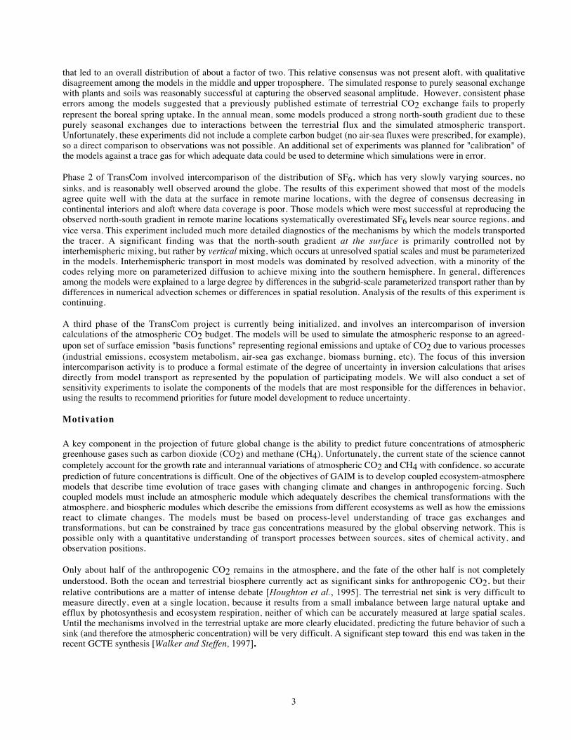
Twelve modelling groups submitted results for Phase 1 of the project. Ten groups submitted results for the SF6experiment (Phase 2), including most of the participants in the TransCom 1 intercomparison as well as several additionalmodels (Table 1). "On-line" models, (CCC, CSU, and GFDL-SKYHI) simulate tracer transport in a fully prognosticgeneral circulation model (GCM), calculating winds and subgrid-scale transport on time steps of minutes. "Off-line" models(CTMs) calculate tracer transport from either analyzed winds (NIRE, TM2) or GCM output (GFDL-GCTM, GISS, GISS-UVic, MUTM, TM3). The off-line models are able to use much longer time steps, and specify input wind fields withfrequencies varying from 1 hour to 1 day. Subgrid-scale vertical transport was parameterized in all models, using a varietyof techniques. Off-line models generally include schemes to calculate these terms from the prescribed wind input, whereasonline models calculate subgrid-scale transports at the same time as the dynamical calculation of the GCM winds. GCMcalculations used on-line winds calculated using climatological sea-surface temperatures as a lower boundary condition. Eachmodel is described in more detail in Appendix 1.

Phase 1: Meridional Gradients and Seasonal CyclesMethod

Two sources of CO2 were chosen for this part of the model intercomparison. The first was the emissions of CO2 due tofossil fuel burning and cement production. This is one of the best known components of the CO2 budget and makes a goodtest of a model’s interhemispheric transport since 95% of the fossil fuel emissions occur in the northern hemisphere. Thesource data used were provided by I. Fung and have been used previously [Tans et al., 1990]. They are based on countryestimates [Andres et al., 1990] which have been distributed within countries according to population density. They includeno temporal variation. The data were provided on a 1 x 1 degree grid with modelers aggregating this to their own modelresolution.

The second source used was the exchange of CO2 with the biosphere. The data were compiled by combining satelliteestimates of photosynthesis with local measurements of respiration and net primary productivity [Fung et al., 1987]. Thesources were validated by comparing modeled (using the GISS model) and observed seasonal cycles of CO2 concentration.This source is the major contributor to the observed seasonal cycle of CO2, at least in the northern extra-tropics. Thussome comparisons can be made between modeled and observed seasonal cycles. There is also considerable interest in theannual mean CO2 field which results from the combination of seasonal sources and seasonal variation in transport.

6

Table 1

TRANSCOM Participating Models - PHASE 1 Parameterized Transport

Model Modeller Type HorizontalResolution

VerticalResolution

Advection Wind Freq Hdiff

Vdiff

Conv

Turb PBL

ANU Tayler Off 2.5˚ 7 pressure Lagrangian ECMWF(80)

Stats Y Y - - -

CSIR 09 Watterson On 3˚x5.6˚ 9 sigma semi-lag. - - - - Y Y -CSU Denning On 4˚x5˚ 17 sigma 2nd order - - - - Y Y Y

GFDL Rayner Off 265 km 11 sigma 2,4 order CFDLGCM

6 hr Y Y - - -

GISS Trudinger Off 8˚x10˚ 9 sigma slopes GISSGCM

4 hr Y - Y - -

MUGCIM Law On R21 9 sigma spectral - - Y Y Y - -MUTM Law Off R21 9 sigma spectral MU GCM 24 hr Y Y Y - -NCAR Erikson On 2.8˚ 18 sigma semi-lag. - - - Y Y - YNIRE Taguchi Off 2.5˚ 15 sigma semi-lag. ECMWF

(92)6 hr - - - - Y

TM1 Piper Off 8˚x10˚ 9 sigma slopes ECMWF(79)

12 hr Y - Y - -

TM2 Heimann Off 4˚x5˚ 9 sigma slopes ECMWF(86)

12 hr - Y Y - -

TM2Z Ramonet Off 2.5˚ 9 sigma slopes ECMWF(90)

12 hr - Y Y - -

Participating Models PHASE 2 Parameterized Transport

Model Modeller Type Reference HorizontalGrid

# Levels Advection Wind Freq HDiff

YDiff

Conv PBL

CCC Holzer GCM McFarlane etal, 1992

3.75˚ 10 sigma/pres

Spectral On-line - Y Y B N

CSU Denning GCM Denning et al,1996

4˚x 5˚ 17 sigma 2nd order On-line - N N C Y

GFDL-GCTM

Fan CTM Mahlman andMoxim, 1978

256 km 11 sigma 2nd order GFDLZODIAC

6 hr Y Y A N

GFDL-SKYHI

Fan GCM Hamilton et al,1995

3˚x3.6˚ 40 sigma 2nd order(horiz),4th(vert)

On-line - Y Y A N

GISS Fung CTM Hansen et al,1997

4˚x 5˚ 9 sigma Slope GISSGCMII

4 hr Y N B N

GISS-UVIC

Fung/Friedlingstein

CTM Hansen et al,1997

4˚x 5˚ 9 sigma Slope GISSGCMII

1 hr N N C N

MUTM Law CTM Law et al,1992

3.3˚x5.63˚

9 sigma Spectral MUGCM7

24hr

Y Y B N

NIRE Taguchi CTM Taguchi et al,1996

2.5˚ 15 sigma/pres

Semi-Lagrangian

ECMWF(93)

6 hr N N N Y

TM2 Bakanski/Bousquet

CTM Bousquet et al,1996

7.5˚x7.5˚ 9 sigma Slope ECMWF(93)

12hr

N Y C N

TM3 Heimann CTM Heimann,1995

3.75˚x 5˚ 19 sigma Slope ECHAM3 GCM

6 hr N Y C N

-Convection Categories:A. Simple DiffusionB. Pair-wise layer MixingC. Penetrative Mass Flux

The experiments, referred to here as the fossil fuel and biosphere experiments, were run for at least three years from aninitial atmosphere with uniform CO2. This provides sufficient time for the model atmosphere to establish "equilibrium"(annually repeating) concentration distributions determined by the surface sources. Contributing modellers suppliedconcentration fields for the surface layer, 500 and 200 mb. In addition, zonal mean cross-sections were analyzed. Each set ofresults has been normalized such that the January global three-dimensional mean is zero.

7

Fossil Fuel Experiment

Differences in interhemispheric transport between models can be seen in the zonal annual mean surface concentrations (Fig.1). While each model gives a broadly similar distribution, with maximum concentrations around 50˚N and relatively smallgradients through the southern hemisphere, there are large differences in the maximum and minimum concentrations. Therange of concentrations found for the northern mid-latitudes can be reduced by almost half if the CSIRO9 and GFDL resultsare excluded. It is likely that this smaller range is more realistic since there have been reported calibrations of meridionalmixing using krypton-85 for the GISS and TM1 models [Heimann and Keeling, 1989; Jacob et al., 1987] which lie inthis range.

The variation among models can be summarized by the interhemispheric concentration difference (northern minus southernhemisphere mean concentration); listed alongside each model identifier in Figure 1. The interhemispheric differences vary bya factor of two. It is important to note that these differences are surface values and the variation between models reflectsdifferences in both vertical and cross-equatorial transport. The CSIRO9 model produces the largest difference (4.7 ppmv) andthe MU models the smallest (2.4 ppmv). In order to understand this difference better, MUTM (an offline model) was runwith winds taken from the CSIRO9 model. This simulation produced an interhemispheric difference of 3.6 ppmv whichindicates that, in this case, the large-scale winds account for about half the difference between the model results with thesub-grid scale parameterizations accounting for the other half.

The qualitative agreement in model responses at the surface breaks down at 200 mb (Fig. 1). Approximately half themodels produce maximum concentrations around 0˚–30˚N while the remainder have mid to high northern latitude maxima.The models that produce the highest surface concentrations in the source region (CSIRO9 and GFDL-GCTM) produceamong the lowest values aloft. This suggests that the high surface values may be more closely related to vertical "trapping"of the tracer in the vicinity of strong emissions rather than weak southward transport. The tropical maxima at 200 mb insome simulations probably result from strong cumulus convection whereas minima in higher latitudes reflect weak verticalmotion. Nakazawa et al.[1991] measured CO2 concentration in the upper troposphere on flights between Tokyo and Sydney(36˚N to 30˚S) and found maximum annual mean concentrations around 0˚–10˚ N. This would be more consistent withthose models that produce low latitude maxima at 200 mb. However, it is important to note that the observed values are forCO2 from all sources whereas the modeled results are for the fossil source only. Also, the model data at 200 mb mayinclude stratospheric air whereas this has been excluded from the observed data. The ANU model produces a more uniformdistribution than the other models. This suggests that there is rapid horizontal mixing acting to reduce the meridionalgradient. Weak vertical mixing could also contribute but this is less likely because the ANU 200 mb global meanconcentration is similar to those from other models.

Biosphere Experiment

The seasonal nature of the biospheric source provides many options for characterizing the models’ responses. We choosehere to focus on the amplitude of the seasonal cycle and the surface annual mean response.

The peak to peak (ptp) amplitudes are calculated as the difference between the maximum and minimum monthly meanconcentration at each grid point. The zonal mean ptp amplitude at the surface (Fig. 2) increases from around 1–2 ppmv inthe southern mid and high latitudes to between 22 and 52 ppmv (32 without CSIRO9 or GFDL) around 65˚N. The largervalues produced by CSIRO9 and GFDL are probably due to slow mixing out of the surface layer. This interpretation isconsistent with the strong meridional gradients produced by these models in the fossil experiment and also with the lowconcentrations these models exhibit at 200 mb above the source region. As in the fossil experiment, the results from theCSIRO9 and MU models are very different. We have also performed the biosphere experiment forcing MUTM with theCSIRO9 winds. The ptp amplitudes that result are almost identical to those produced by MUTM (forced with MUGCMwinds), particularly in the northern mid and high latitudes. This suggests that the sub-grid scale parameterizations controlthe amplitude of the seasonal cycles at these latitudes.

Figure 2 shows the amplitude of the seasonal cycle at Barrow, and the surface monthly mean concentration for each modelat this site. Also shown is the observed seasonal cycle represented by the first two harmonics fitted to detrended data fromConway et al., [1994]. In general there is close agreement between models in the structure of the seasonal cycle althoughthere are large discrepancies in the magnitudes of the maximum and minimum concentrations. Comparison of the modelswith the observed seasonal cycle reveals some systematic problems, however. All models produce a maximum value which

8

is too large and occurs too late. The winter concentrations are too low but the August-November period is reasonablysimulated. Since all the models are producing similar errors, this suggests an error with the input sources rather than withthe model transport, particularly as similar discrepancies are seen at most of the high northern latitude sites. Low light andlong atmospheric path lengths result in errors in the NDVI (and hence CO2 fluxes) at high latitudes in Spring. There mayalso be errors in the respiration estimates through the use of air temperatures rather than soil temperatures. This illustratesthe potential extra information that can be gained by running a range of transport models. Had only one result beenavailable it would be more difficult to distinguish between source and transport errors.

Surface 200 mb

Latitude Latitude

Figure 1: Zonal mean annual mean mixing ratio of CO2 response to fossil fuel emissions assimulated by 12 tracer transport models. The value at the south pole has been subtracted. The left panelshows the response at the Earth's surface (or in the lowest model layer), and the right panel shows theresponse at the 200 mb pressure level. Note that the CSIRO9, GFDL-GCTM, and ANU models,behaved differently from the others.

While the annual mean biospheric source is zero everywhere, this is not true of the spatial distribution of annual meanconcentration resulting from this source. The interaction of seasonal variations in transport with the seasonal sourceproduces non-zero annual mean concentrations. The zonal annual mean (Fig. 3) shows that for some models (CSIRO9,CSU, GFDL, NCAR and NIRE) the north-south gradient is around half that produced in the fossil experiment. Mostmodels produce small positive concentrations around the equator. These result from the seasonal shift of the InterTropicalConvergence Zone (ITCZ). The positive concentrations in the northern mid-latitudes appear to be more associated withseasonality in vertical transport. For example, experiments with MUTM have shown that seasonality of convection isimportant.

The annual mean response of the ANU model is qualitatively different from the other models. Taylor (pers. comm.) hasindicated that the negative concentrations result from the use of 1980 winds at only 7 levels; small positive concentrationswere obtained in subsequent experiments when winds from the 1990s at 14 or 15 levels were used. When the ANUCSIRO9 and GFDL-GCTM models (which appear to exhibit unrealistic vertical trapping) are removed (Fig. 3), theremaining results cluster into two populations. Models with explicit formulations of vertical mixing in a variable-depthplanetary boundary layer exhibit strongly elevated annual mean surface concentrations over the northern hemisphere,whereas the others do not. It is likely that the seasonality of the Planetary Boundary Layer (PBL) depth contributes to thepositive annual means due to "rectification" of the seasonal fluxes [Denning et al., 1995; Keeling, 1989; Taguchi, 1996].The ability to resolve changes in vertical mixing due to the diurnal cycle may also be important [Denning et al., 1996].

9

Zonal Mean Amplitude Phase at Barrow, Alaska

Latitude

Figure 2: Seasonal cycle of CO2 response to terrestrial exchange fluxes of Fung et al. [1987]simulated by 12 atmospheric tracer transport models. The left panel shows zonal mean annual peak-to-peak amplitude at the surface; right panel shows monthly mean surface values for the grid cellcorresponding to Point Barrow, Alaska, with circles indicating the observed seasonal cycle [Conway etal., 1994].

Terrestrial Biosphere ExperimentAll Models "Outliers" Removed

Latitude Latitude

Figure 3: Annual mean zonal mean surface CO2 mixing ratio response to purely seasonal exchangewith the terrestrial biosphere as simulated by 12 atmospheric tracer transport models. The left panelshows all the models. The right panel is identical except that the "outlier" models have been removed.

10

Conclusions from Phase 1

We have compared the simulation of CO2 concentration due to fossil fuel emissions and biospheric exchange by 12atmospheric tracer transport models. While each model produces broadly similar concentration distributions there is a largerange in the efficiency of transport among models. For example, surface interhemispheric exchange times varied by a factorof two, although this range can be significantly reduced by removing a few outlier responses.

The implications of these results for CO2 budget studies are substantial. In addition to the range in meridional gradientproduced by the fossil experiment, there is no clear consensus among models on the annual mean response to the biosphereexchange. The uncertainties in transport produce uncertainties in regional carbon budgets comparable to those from otherelements of the inversion. Uncertainties in transport can also be expected to impact modelling of other chemical species inthe atmosphere whenever the lifetime is long enough for transport to affect the distribution of the species. More detailedobservations of CO2 and other species, particularly aloft and over the continents, can play a major role in constraining bothtransport and net sources.

Phase 2: Calibration and Diagnosis with SF6

Sulfur hexafluoride is an anthropogenic trace gas with an atmospheric lifetime of over 3000 years [Ravishankara et al.,1993], whose mixing ratio is increasing rapidly in the troposphere [Geller et al., 1997; Levin and Hesshaimer, 1996; Maissand Levin, 1994; Maiss et al., 1996]. It is believed to be emitted by slow leakage primarily from electrical switchingequipment, which is its main industrial use. Its time series is very "clean" and easy to interpret. Unlike other anthropogenictracers such as CFCs and krypton-85, the rate of global emissions is relatively steady, so the annually averagedconcentration field is in a quasi-stationary state (Fig. 4). The global source has been estimated from the time series of itsmixing ratio at various locations using archived air samples [Maiss et al., 1996]. The spatial pattern of SF6 mole fractionat the surface is reasonably well characterized by a set of flask sampling programs and by intensive sampling programs, andthe sampling density is growing rapidly.

Experimental Method

The experiment consisted of integrating each model surface forcing of SF6 emissions prescribed as closely as possible tothe real values, and saving model data corresponding to observations. We also saved a suite of diagnostic fields forcomparison from model to model.

Emissions of SF6 were prescribed according to the global estimates [Levin and Hesshaimer, 1996]. These global estimateswere linearly interpolated to daily values defined on the fifteenth of each month between December 1988 and January 1994to avoid “shocks” associated with changing emission rates at year boundaries. The global emissions were distributedgeographically on a 0.5° x 0.5° grid, according to electrical power usage by country [United Nations, 1994] and populationdensity [Tobler, 1995]. This distribution reflects the predominant electronical equipment source of SF6 to the troposphere.Each participating group then computed the area-weighted average of the emissions distribution onto their (coarser) modelgrid, and scaled the values to preserve the global integrity.

The models were initialized with a globally uniform tracer distribution for January 1, 1989. An initial condition of 2.06parts per trillion by volume (pptv) was specified, using the model of Maiss et al., [1996]. Each model then integrated thetracer calculation for 5 years, updating the emissions field daily, ending on December 31, 1993. Results were archived forthe final 12 months of the integration, and each group submitted a large set of simulated tracer statistics and transportdiagnostics, as described below.

Diagnostic output was designed to provide both an opportunity to compare the simulated SF6 abundance toobservational data, and to elucidate mechanisms for the different behavior of the model simulations. Our experience inTransCom Phase 1 suggested that this would require information about both resolved advective transport and subgrid-scaleparameterized transport. Interpolation of transport diagnostics to pressure coordinates and the use of vertically integratedmass transport slabs was intended to allow budgets to be estimated and to allow quantitative comparison of the variouscomponents of such budgets. Resolved advection was calculated in terms of mass fluxes, and subgrid-scale parameterizedtransport was

11

Fig

ure

4

12

presented as tendencies. Mass fluxes were calculated from "local anomaly" mixing ratios ( 0CCC −≡+ ) after subtracting

the global mean (background) mixing ratio of sulfur hexafluoride (C0), to provide a more robust estimate of the divergenceof the advective transport.

Observational data

Observational data used to evaluate model performance were gathered from a number of sources representing various timeperiods and frequencies (Fig. 5). Time series of SF6 mole fraction from continuous analyzers and archived air samples wereavailable for five stations representing the remote troposphere at latitudes from 83° N to the Antarctic coast over timeperiods ranging from one to twenty-five years [Levin and Hesshaimer, 1996; Maiss et al., 1996]. A meridional profile wasobtained from measurements taken during a cruise in the Atlantic Ocean during October/November 1993 [Maiss et al.,1996]. Flask samples from a subset of the NOAA-CMDL network have been analyzed for SF6 since early 1996 (E.Dlugokencky and P. Tans, personal communication). Hourly time series of SF6 have been measured along with a suite ofother trace gases near the top of tall television towers in North Carolina (WITN-TV) and Wisconsin, USA (WLEF-TV)since 1994 [Hurst et al., 1997]. Two SF6 transects across Eurasia from Moscow to Vladivostok were measured during 1996by Crutzen et al., [in press] on the Trans-Siberian Railroad. Many of the observational data have become available since theexperimental protocol was developed. The rapid accumulation rate of SF6 in the troposphere precludes the direct comparisonof these data to the model simulations for 1993. Data collected in other years was extrapolated in time to 1993 forcomparison to models by one of two methods (Table 2): (1) data from sites with sufficiently long time series wereextrapolated using a linear trend determined from the data; and (2) other data were extrapolated using the quadratic fit to theglobal mean trend suggested by Maiss et al., [1996].

Heidelberg data (Maiss et al, 1996)

Atlantic Transect, November 1993 (Maiss et al, 1996)

Trans-Siberian Railroad Transect (Crutzen et al, 1997)

NOAA-CMDL Flask Data (E. Dlugokencky and P. Tans, per. comm)

Figure 5: Locations of Stations Compared to Models.

13

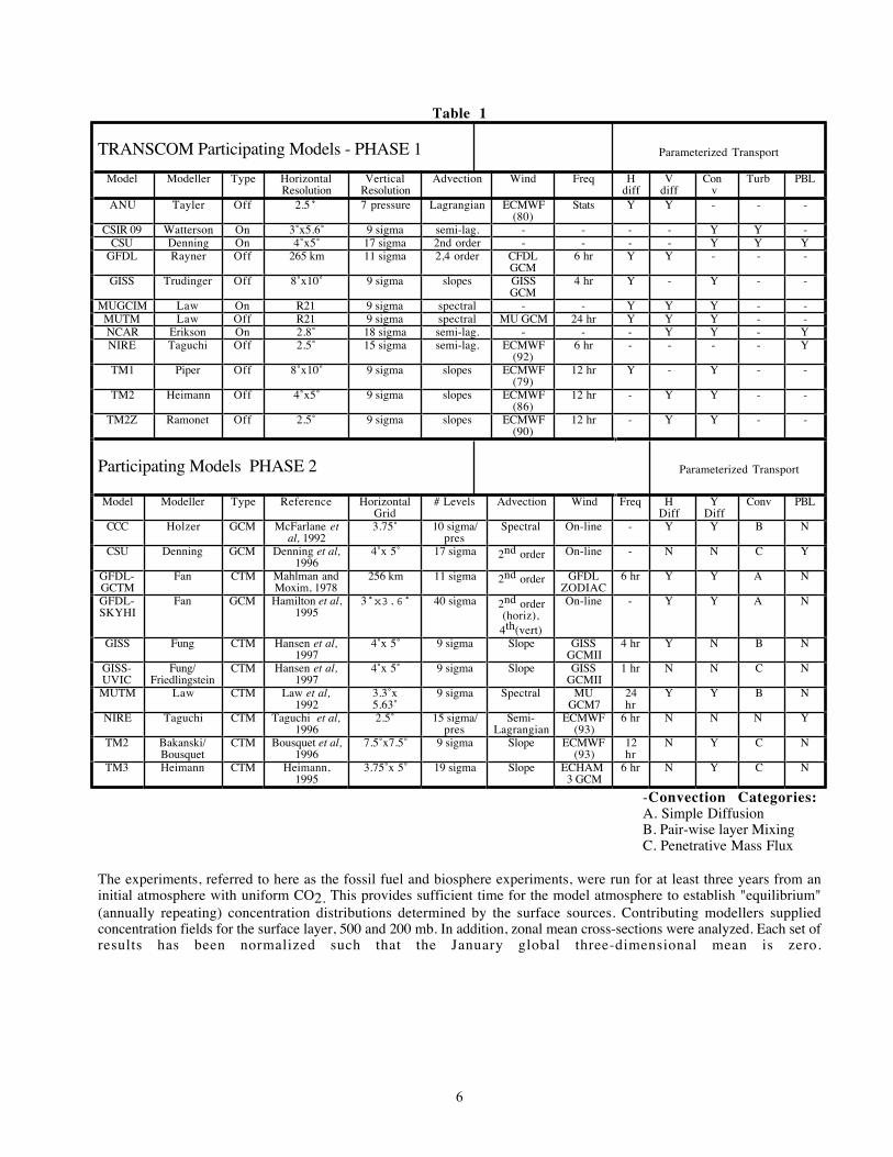
Table 2. SF6 mole fraction at measurement sites: observations and model simulations.

Simulated Surface Mixing Ratio: Comparison to Observations

Simulated surface mole fractions display a pole-to-pole difference of about 10% (0.3 pptv) from the Arctic to the Antarctic(Fig.6). Most of the models are reasonably successful in capturing the observed magnitude of this meridional gradient, withconsiderably less model-to-model variance than was apparent in the zonal mean distributions presented in TransCom 1 [Lawet al., 1996]. This may be due to improvements in some of the models since the earlier experiment, and may also reflectthat one model (CSIRO9) which produced much stronger than average meridional gradients at the surface was not includedin TransCom 2. Less variation is expected for "clean air" sites in the marine boundary layer than the surface zonal meanswhich were compared in TransCom 1. The elevated SF6 values at Kumukahi and the Azores may be an artifact introducedby the extrapolation of data collected in 1996 back in time to compare to the 1993 simulations.

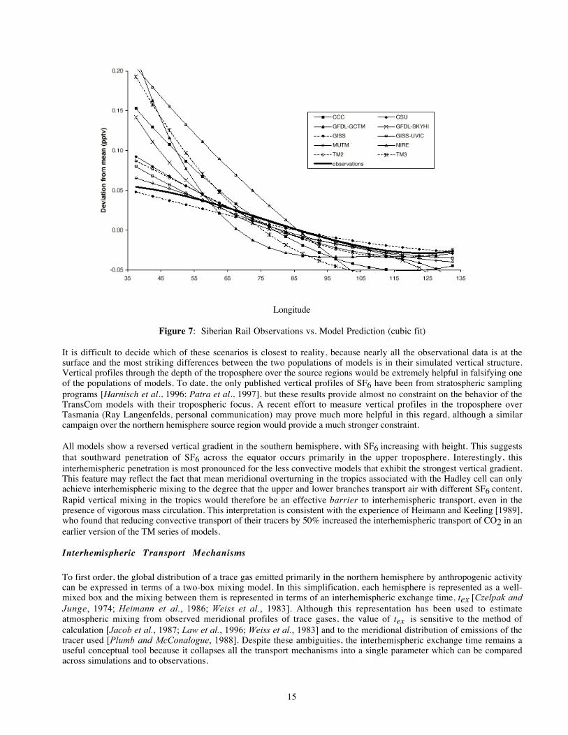
An additional observational constraint on the degree of tracer accumulation in the source regions is provided by thelongitudinal gradient through the "plume" of elevated SF6 concentrations extending eastward from the European sourceregion across Eurasia. The models with the highest concentration maxima (NIRE, GFDL-GCTM, TM3, and possiblyCCC) all overestimate the gradient between Moscow and central Siberia as measured by the railroad transect [Crutzen et al.,1997] (Fig. 7). This could be indicative of insufficient advective transport in the vicinity of strong horizontal concentrationgradients. Alternatively, it could indicate excessive vertical trapping, as shown by the higher global mean surface molefractions in these models as discussed above. Horizontal redistribution cannot account for these differences in the globalmean surface mole fraction.

Meridional profiles of surface concentrations of anthropogenic tracers have frequently been interpreted in terms of meridionaltransport and interhemispheric exchange. Such an interpretation is complicated for the results presented here because boththe simulations and the observations show considerable longitudinal variation. Interhemispheric gradients estimated fromthese data will depend strongly on the locations of observing stations, and may reflect the degree to which tracer mass isretained in the source regions against zonal or vertical mixing as well as meridional mixing. We note that the area-weightedglobal surface mean mole fractions are significantly lower for those models with the weakest meridional gradients (CSU,MUTM, GISS) than for those with the strongest gradients (NIRE, GFDL-GCTM, TM3).

14

Latitude

Figure 6: Marine Boundary Layers (MBL) Surface SF6 Observations (time adjusted) and ModelPredictions (emissions adjusted).

None of the models simultaneously satisfies the constraints of the meridional gradient in the marine boundary layer and thelongitudinal gradient across Eurasia. This could be accomplished by more vigorous horizontal transport in the lowertroposphere, reducing regional maxima in the regions, and increasing values in the remote Marine Boundary Layers (MBL).The "less convective" models would have to compensate by allowing more vertical mixing of traver to preventoverestimating the MBL data. Similarly, the "more convective" models would have to have reduced vertical mixing toprevent underestimates of the east-west gradient.

Zonal Mean Vertical and Meridional Structure

Zonal mean cross-sections of annual mean simulated mole fraction for each model are compared in Figure 8. All modelsshow elevated mole fractions at the surface in the northern hemisphere source region. The models can be classified into twopopulations based on these cross-sections: one group (CSU, GISS, MUTM, and TM2) simulates relatively weak verticalgradients over the northern extra tropics, whereas a second group (CCC, both GFDL models, GISS-UVic, TM3, andespecially NIRE) simulate stronger vertical gradients over the source region. This probably reflects differences in thesubgrid-scale parameterized transport be convection and diffusion.

The division of the models into a "strongly mixed" and a "weakly mixed" population also seems to explain many of thedifferences in simulated surface tracer distributions discussed above. The weakly mixed models tend to accumulate more SF6in the lower troposphere of the northern hemisphere, and thus have stronger surface meridional gradients than the stronglymixed models. The most strongly vertically mixed models (CSU GISS, MUTM) tend to underestimate the surface molefraction at most observing stations (cf. Fig. 6). The more weakly mixed models (NIRE, TM3, and the GFDL models) aregenerally quite successful at simulating the observed meridional gradient in the remote marine boundary layer (Fig. 6), butsystematically overestimate SF6 at continental sites and near the western end of the Siberian transect (Fig. 7). These resultssuggest that differences in parameterized vertical transport among the models, rather than differences in resolved advection,may account for most of the differences in meridional structure at the surface.

15

Longitude

Figure 7: Siberian Rail Observations vs. Model Prediction (cubic fit)

It is difficult to decide which of these scenarios is closest to reality, because nearly all the observational data is at thesurface and the most striking differences between the two populations of models is in their simulated vertical structure.Vertical profiles through the depth of the troposphere over the source regions would be extremely helpful in falsifying oneof the populations of models. To date, the only published vertical profiles of SF6 have been from stratospheric samplingprograms [Harnisch et al., 1996; Patra et al., 1997], but these results provide almost no constraint on the behavior of theTransCom models with their tropospheric focus. A recent effort to measure vertical profiles in the troposphere overTasmania (Ray Langenfelds, personal communication) may prove much more helpful in this regard, although a similarcampaign over the northern hemisphere source region would provide a much stronger constraint.

All models show a reversed vertical gradient in the southern hemisphere, with SF6 increasing with height. This suggeststhat southward penetration of SF6 across the equator occurs primarily in the upper troposphere. Interestingly, thisinterhemispheric penetration is most pronounced for the less convective models that exhibit the strongest vertical gradient.This feature may reflect the fact that mean meridional overturning in the tropics associated with the Hadley cell can onlyachieve interhemispheric mixing to the degree that the upper and lower branches transport air with different SF6 content.Rapid vertical mixing in the tropics would therefore be an effective barrier to interhemispheric transport, even in thepresence of vigorous mass circulation. This interpretation is consistent with the experience of Heimann and Keeling [1989],who found that reducing convective transport of their tracers by 50% increased the interhemispheric transport of CO2 in anearlier version of the TM series of models.

Interhemispheric Transport Mechanisms

To first order, the global distribution of a trace gas emitted primarily in the northern hemisphere by anthropogenic activitycan be expressed in terms of a two-box mixing model. In this simplification, each hemisphere is represented as a well-mixed box and the mixing between them is represented in terms of an interhemispheric exchange time, tex [Czelpak andJunge, 1974; Heimann et al., 1986; Weiss et al., 1983]. Although this representation has been used to estimateatmospheric mixing from observed meridional profiles of trace gases, the value of tex is sensitive to the method ofcalculation [Jacob et al., 1987; Law et al., 1996; Weiss et al., 1983] and to the meridional distribution of emissions of thetracer used [Plumb and McConalogue, 1988]. Despite these ambiguities, the interhemispheric exchange time remains auseful conceptual tool because it collapses all the transport mechanisms into a single parameter which can be comparedacross simulations and to observations.

16

Figure 8: Annual and Zonal Mean SF6 Mole Fraction (pptv)

17

Critical to the assessment of interhemispheric exchange time is the way in which the hemispheric mixing ratios arecomputed. Table 3 shows tex based on both model results and measurements comprising different definitions of thehemispheric mean SF6 mixing ratios. Interhemispheric exchange times were calculated both for the October-Novemberperiod, to facilitate comparison with the observational tex from the Atlantic transect, and as annual means, which are morerepresentative of overall model performance. To highlight relative differences among the models, the annual mean texvalues are also indicated in terms of their "rank," with fastest interhemispheric transport indicated by 1 and the slowest by10.

Table 3. Interhemispheric Transport Comparison

(tex in years)

October/November Annual

S-S tex (1-D) tex (1-D) tex (2-D) tex (3-D) tex (1-D) Rank tex (2-D) Rank tex (3-D) Rank

CCC 1.31 1.88 1.53 0.57 1.14 5 1.53 5 0.58 2

CSU 0.90 0.91 1.01 0.66 0.90 2 1.18 2 0.72 4

GFDL-GCTM 1.46 2.06 1.51 0.71 1.32 6 1.66 6 0.83 6

GFDL-SKYHI 0.92 0.91 1.21 0.69 1.05 4 1.44 4 0.73 5

GISS 0.90 0.96 1.15 0.84 1.00 3 1.22 3 0.88 8

GISS-UVIC 1.47 1.76 1.97 1.40 1.60 8 1.95 8 1.28 10

MUTM 0.76 0.82 1.03 0.57 0.82 1 1.12 1 0.63 3

NIRE 1.98 3.93 2.46 1.06 1.72 10 1.95 9 0.84 7

TM2 1.42 2.08 2.24 0.56 1.33 7 1.75 7 0.50 1

TM3 1.60 1.93 2.01 1.20 1.54 9 1.99 10 1.04 9

Observations 1.34

In the first case, labeled "S-S tex (1-D)", the hemispheric mean SF6 mixing ratios were computed based onOctober/November 1993 Atlantic transect SF6 measurements. All the measurement locations north (south) of the equatorwere averaged (weighted by the cosine of latitude) to achieve the northern (southern) hemisphere mean SF6 mixing ratios.The monthly mean 1993 model predictions for the Atlantic measurement locations were retrieved and interpolation betweenthe October mean and the November mean were made to achieve a value consistent with the transect measurement dates.As can be seen in the table, this leads to interhemispheric exchange times of roughly one to two years for both the steady-state case and the instantaneous case (labeled "tex (1-D)". Note that this is the method used to estimate interhemisphericexchange from field programs, and that it implicitly assumes that each point measurement is both zonally and verticallyrepresentative. Figure 8 clearly demonstrates that this is not the case for SF6 in the models. The assumption that verticaland longitudinal variations can be neglected in the calculation of a two-box mixing time is probably quite unrealistic innature as well.

The average hemispheric SF6 mole fractions were also computed as surface-area weighted means (for the models only), andused to calculate an exchange time labeled "tex (2-D)" in the table. The interhemispheric exchange time calculated from allsurface locations is larger than the one-dimensional case for all the models. This reflects the higher mole fractions inlongitudinal regions strongly influenced by SF6 source areas such as the eastern portion of North America and WesternEurope. The interhemispheric exchange time calculated in this way implicitly assumes that each surface point represents a

18

column mean. Note that the ranking of the tex values among models changes very little in going from station-based 1-Destimation to the full 2-D surface global mean mole fractions. The only change in the relative strengths of apparentinterhemispheric exchange from the 1-D to 2-D cases is that NIRE and TM3 have switched positions for the slowest amongthe suite of models.

The extent to which tex increases over the one-dimensional case also reflects the magnitude with which the models mixSF6 zonally and vertically. For example, those models that exhibit strong vertical mixing exhibit two-dimensional textimes that are less affected by the inclusion of source regions in the northern hemisphere mean SF6 mole fraction, becausethey retain less tracer near the surface in the source regions. Hence, their two-dimensional tex times do not increase asmuch over the one-dimensional case as is the case for those models with less vigorous vertical mixing. This is supportedby the relative change in tex for the GISS and GFDL-SKYHI models. Both models have a nearly identical one-dimensionaltex time yet the two-dimensional values diverge with the more vertically-mixed model, GISS, increasing to a tex of 1.22years versus the larger GFDL-SKYHI value of 1.44 years.

In addition, tex was estimated by incorporating three-dimensional, mass-weighted mean mixing ratios for the northern andsouthern hemispheric mean SF6 values. Interhemispheric exchange times derived in this way are true to the spirit of thetwo-box mixing model in that they represent the true hemispheric mean concentrations in each box, but still violate thewell-mixed assumption. Not surprisingly, the interhemispheric exchange times calculated from 3-D means are much lowerthan their 2-D analogs, reflecting both the lesser absolute mixing ratio in the northern hemisphere and the diminishedinterhemispheric gradient of SF6 aloft in all the models.

Using the full three-dimensional hemispheric means to calculate the two-box exchange time produces shifts in the relativeintensity of inferred interhemispheric exchange among the models. These changes are much more significant than thechanges in the relative ranks among models in going from a 1-D calculation to a 2-D calculation. Models that exhibitgenerally greater vertical mixing tend to have the lowest tex values (CSU, MUTM, and GISS), but some models behavevery differently in 3-D than we inferred from 2-D means. The CCC model has one of the slowest exchange times asestimated from surface gradients, yet is one of the fastest when true mass-weighted means are used. The GISS-UVic model,on the other hand, exhibits the slowest tex in 3-D, though has only the fourth-fastest tex in 2-D. NIRE has by far theslowest tex when surface means are used, yet is faster than either GISS-UVic or TM3 when the full mass-weightedhemispheric mean values are used.

The exchange time estimated from surface values, especially at only a small number of longitudes, is clearly a poorpredictor of true interhemispheric mixing in these models. The fact that the relative intensity of interhemispheric mixing isnearly unchanged from the 1-D to the 2-D case, but changes dramatically from the 2-D case to the 3-D case indicates thatdifferences in vertical structure among the models dominate the differences in true interhemispheric exchange.

Interhemispheric exchange time was also estimated for many of the same models from the fossil fuel experiment inTransCom 1 [Law et al., 1996]. In general, most models that participated in both experiments showed slower exchangetimes for SF6 than for fossil fuel CO2. This must be interpreted with care however, because (1) several of the models havebeen modified significantly between the two experiments, and (2) Law et al. [1996], used a steady-state approach tocalculate the exchange times. Nevertheless, our results confirm the general TransCom 1 results of Law et al., [1996]: texincreases from station-based 1-D estimates to a full 2-D surface mean, but using the full 3-D mass-weighted mean mixingratios produces the fastest exchange time estimates. The increase from estimates based on data collected in the remote MBLto the 2-D estimate reflects the inclusion of regional concentration maxima in source regions, and the decrease from 2-D to3-D estimates removes the confounding effects of vertical tracer gradient that can so easily be misinterpreted as meridionalgradients.

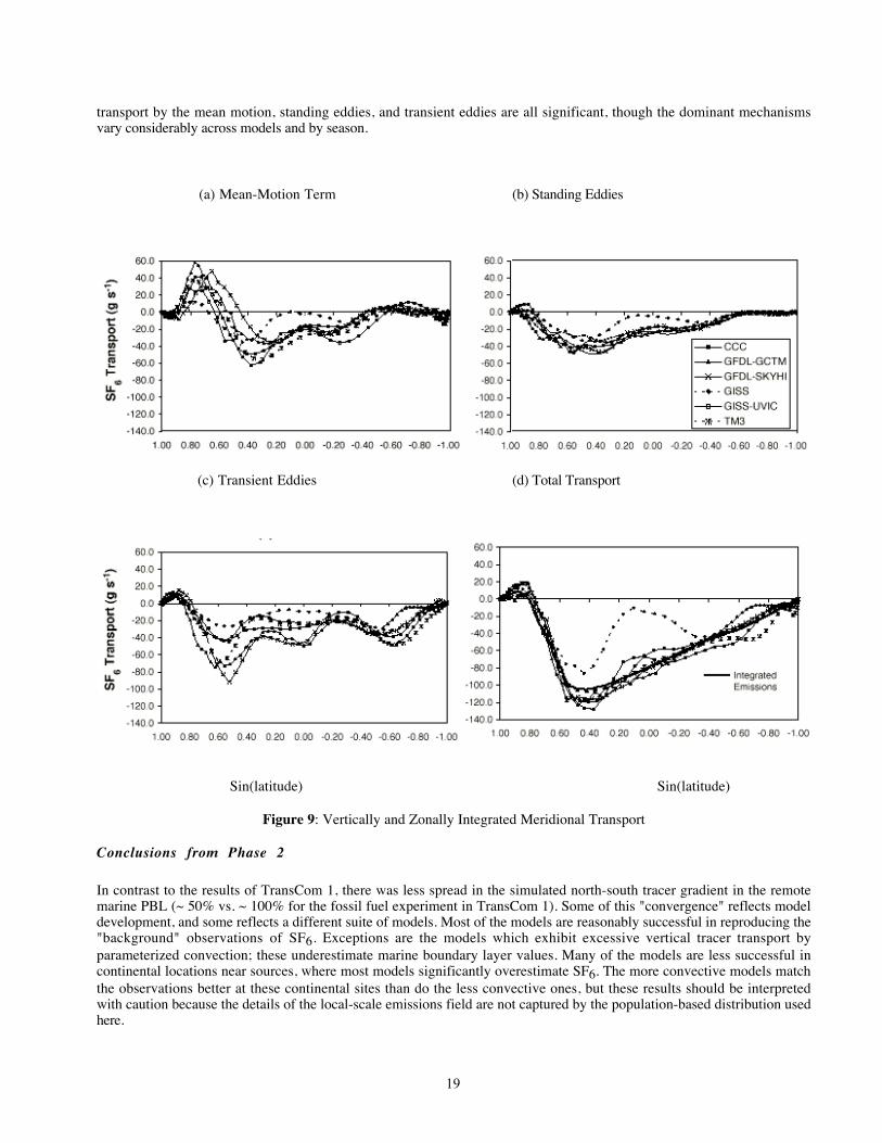
Another approach to the diagnosis of interhemispheric transport is to decompose the total meridional tracer transport intocontributions by the time-averaged zonal mean motion (e.g., by the Hadley and Ferrel Cells); the standing eddies (time-averaged deviations from the zonal mean that span a range of longitudes, such as blocking highs, the Aleutian low, and theAsian Monsoon); and the transient eddies (deviations in both space and time from the mean flow, such as those caused bywinter storms in the middle latitudes). We performed this decomposition for a subset of the SF6 simulations (Fig. 9). Thetotal column integrated resolved meridional transport is not very different among the models, and is in fact constrained tobalance the integrated surface emissions. The only major exception to this statement is the GISS model, whichaccomplishes much of its meridional transport via parameterized subgrid-scale horizontal diffusion. In all cases, meridional

19

transport by the mean motion, standing eddies, and transient eddies are all significant, though the dominant mechanismsvary considerably across models and by season.

(a) Mean-Motion Term (b) Standing Eddies

(c) Transient Eddies (d) Total Transport

Sin(latitude) Sin(latitude)

Figure 9: Vertically and Zonally Integrated Meridional Transport

Conclusions from Phase 2

In contrast to the results of TransCom 1, there was less spread in the simulated north-south tracer gradient in the remotemarine PBL (~ 50% vs. ~ 100% for the fossil fuel experiment in TransCom 1). Some of this "convergence" reflects modeldevelopment, and some reflects a different suite of models. Most of the models are reasonably successful in reproducing the"background" observations of SF6. Exceptions are the models which exhibit excessive vertical tracer transport byparameterized convection; these underestimate marine boundary layer values. Many of the models are less successful incontinental locations near sources, where most models significantly overestimate SF6. The more convective models matchthe observations better at these continental sites than do the less convective ones, but these results should be interpretedwith caution because the details of the local-scale emissions field are not captured by the population-based distribution usedhere.

20

Our results generally agree with the TransCom 1 findings that strong meridional gradients in simulated fossil fuel CO2 atthe surface were systematically associated with weak meridional gradients in the upper troposphere, and vice versa. Inaddition, the importance of vertical transport for interpreting observed meridional structure at the surface was underlined bythe TransCom 1 biosphere experiment, which showed that models with a large degree of vertical trapping of fossil fuelCO2 exhibited stronger than observed meridional gradients in the amplitude of biospheric CO2.

Although there are distinct differences in the intensity of interhemispheric exchange among the models, these differencescannot be understood in terms of spatial distributions of tracer at the surface. The ranking of estimated tex using 1-Dstation data or the 2-D surface global mean mole fraction is nearly the same, whereas the true tex calculated from 3-Dmass-weighted mean mole fractions produces an entirely different ranking. This result confirms that differences ininterhemispheric exchange times among the models are dominated by differences in vertical structure. Observed meridionalgradients of tracers should be interpreted with caution, since a two-box mixing model derived from surface observations canclearly produce qualitatively false results in which vertical mixing is misconstrued as interhemispheric transport.

Modelling the Methane Cycle

In addition to applications to non-reactive trace gases, insights provided by the results of the Transport CodeIntercomparisons will set the stage for developing models of the methane cycle. Methane has been identified as a majorclimate gas in the atmosphere and a key compound in the chemical processes affecting tropospheric ozone chemistry. Therecent 1995 IPCC assessment has strongly upgraded its climatic role compared to previous assessments, mainly due to itschemical impact on the atmosphere. Measurements have clearly demonstrated that its atmospheric concentration has beenincreasing over the last century, and is now believed to be more than a factor of two higher than the pre-industrial values.This increase has undoubtedly had a profound impact both on climate and atmospheric chemistry. Methane has increasedover the last decade by 0.8% per year on average, while the rate over the last few years has been substantially less. Thecause of the long term trend, and the decrease in recent years are not fully understood. Both could be either the result ofchanges in the magnitude of surface sources or in the atmospheric sinks. Anthropogenic sources of methane are related toagricultural and industrial activities. In particular, there is poor quantification of the potential changes in soil emissions andconsumption associated with changes in land-use and other modifications in terrestrial ecosystems.

Methane is simpler in one respect than the CO2 cycle in that it does not have large and poorly constrained sinks in theocean and terrestrial systems. However, methane is not conservative in the atmosphere, being subject to oxidation. Theatmospheric chemical interaction of methane is being studied in a joint GAIM/IGAC 3-D model intercomparison activity.This study focuses on the atmospheric response to changes in emissions, and therefore links naturally to the proposedmethane cycle study. For instance, 3-D model estimates of temporal and spatial variations of methane oxidation can be usedtogether with observed variations of methane to estimate emissions from wetlands.

As a first step in exploring the methane cycle, we have focused on terrestrial sources, the largest of which are natural andartificial wetlands. The methane budget is strongly affected by wetland sources, both natural and anthropogenic.Consequently, in order to correctly account for methane terms in global biogeochemical models, it is essential to understandthe role of wetlands in methane production as well as the effect of changing wetland distribution. The extent of wetlands isuncertain because there is no clear basis for identification and functional classification of wetlands on a global scale. Inaddition, the areal extent of wetlands is being modified as a result of land-use changes, so that once a globally consistentclassification scheme is established, the areal distribution must be monitored and recompiled. New data are becomingavailable from remote sensing which provide a global perspective on wetland distribution and classification, but which arenot yet reconciled with ground-based ecological and hydrological data. There remains a gulf between the scale of trace gasemissions as measured from the ground, and the measurable atmospheric effects of this based on remote sensing. Theseconceptual and technical discontinuities need to be reconciled.

As a first step, we have constructed a wetland functional classification scheme [Sahagian, 1998]. This, in conjunction withdevelopments in understanding of emissions from rice paddies and ruminants will provide the input boundary flux foratmospheric methane necessary for climate and biogeochemical models. This flux will be balanced against oxidation andatmospheric accumulation, as modulated by atmospheric transport, to be provided by the transport codes as tested in Phase1.

With sources, sinks, and atmospheric transport terms in hand, methane cycle models can be subsequently developed whichwill accurately predict atmospheric methane concentration evolution in response to human activity as well as naturalcauses.

21

General Conclusions

We have made significant progress in understanding the mechanisms for differences among the models. Our resultsunderline the importance of subgrid-scale parameterized vertical transport, even for the interhemispheric transport of a long-lived passive tracer. Differences in the meridional gradient of SF6 at observing sites in the remote marine boundary layeramong models cannot be explained in terms of differences in meridional transport or interhemispheric mixing. Rather, acombination of vertical and meridional transport is involved, with meridional gradients at the surface associated with strongvertical gradients in the source regions. The differences among models are best explained in terms of differences in theintensity of subgrid-scale parameterized vertical transport rather than in terms of distinctions between CTMs and GCMs, orthe use of analyzed wind observations rather than GCM simulated winds for the resolved transport.

The vertical distribution of atmospheric trace gases is much more difficult and expensive to quantify through observingprograms than is the horizontal spatial structure at the surface. Observational data collected at the surface may easily bemisinterpreted in terms of meridional transport and interhemispheric mixing unless a better constraint is placed on verticalprofiles in areas of elevated surface concentrations and on meridional gradients aloft. A series of regular vertical profiles ofSF6 over western Europe and the northeastern United States would provide a useful constraint for model validation. If sucha program were combined with periodic meridional profiles in the middle to upper troposphere, it would be feasible tofalsify one or the other of the two "families" of simulations considered here.

We note that both TransCom 1 and TransCom 2 have found significant differences in simulated meridional and especiallyvertical tracer structure that result entirely from differences in the simulated transport among models. Some of the models inthese experiments are also being used to simulate the distribution of reactive trace gases in the troposphere, andinterpretation of the results of such experiments must be done with caution since transport differences are involved withdifferences in reactive chemistry in such experiments. A systematic program to quantify the 3-dimensional distribution ofan easy-to-measure nonreactive tracer such as SF6 would be prudent to allow the simulated transport to be calibrated amongthese models. Such a program would add significant value to observing programs which measure reactive gases.

One important aspect of the transport model incorporation was the striking difference between models in the simulatedsurface meridional gradient of CO2 in the TransCom 1 biospheric experiment. The Arctic-to-Antarctic CO2 gradient in thatexperiment varied from 2.5 ppm in models with strong rectification (CSU, CCM2, NIRE) to less than 0.5 ppm for thosemodels with weak rectification (GISS, MUTM, TM2), to -1.5 ppm for the ANU model, which appears to exhibit negativerectification [Law et al., 1996]. This important difference has a direct and significant bearing on the use of these models inCO2 inversion studies [Denning et al., 1996; Denning et al., 1995]. Unfortunately, neither the SF6 experiment nor a222Rn calibration can directly address the question of rectification. Correct vertical transport by subgrid-scale processes is anecessary condition for correct simulation of rectification, and can be tested with better data on the vertical and seasonalchanges in tropospheric 222Rn. Terrestrial CO2 flux is different from 222Rn in that it changes sign from night to day andfrom summer to autumn; it is the covariance between flux and the vertical transport that must be simulated correctly.Calibrating this aspect of model transport may best be accomplished at smaller scales using intensive field data rather thanglobal simulations using occasional and widely scattered column constraints.

The use of tracer transport codes for atmospheric inversion studies is a valuable tool that can add significant informationabout sources and sinks of atmospheric trace gases. Such calculations currently face considerable uncertainty due todifferences in simulated transport. Future activities will seek to quantify the uncertainty in carbon cycle inversioncalculation arising from the transport directly, through an inversion intercomparison.

22

References:

Andres, R.J., G. Marland, I. Fung, and E. Matthews, A 1-degrees-X1-degrees distribution of carbon dioxide emmisionsfrom fosil fuel consumption and cement manufacture, Global Biogeochemical Cycles, 10, 419-429, 1990.

Ciais, P., P. Tans, J. White, M. Trolier, D. Schimel, and others, Partitioning of Ocean and Land Uptake of CO2 asInferred by Delta-C-13 Measurements from the NOAA Climate Monitoring and Diagnostics Laboratory Global AirSampling Network, J. Geophys. Res., 100, 5051-5070, 1995.

Conway, T.J., P. Tans, L. Waterman, K. Thoning, D. Buanerkitzis, K. Masarie, and N. Zhang, Evidence for interannualvariability of the carbon cycle from the NOAA/CMDL global air sampling network, J. Geophys. Res., 99D, 22831-22855, 1994.

Crutzen, P., T. Rockmann, C. Brenninkmeijer, and P. Neeb, Ozonolysis of nonmethane hydrocarbons as a source of theobserved mass independent oxygen isotope enrichment on tropospheric CO., J. Geophys. Res., 103, 1463-1470, 1998.

Crutzen, P.J., N.F. Elansky, M. Hahn, M. Golitsyn, and others, Trace gas measurements between Moscow andVladivostok using the Trans-Siberian Railroad, Atmos. Chem., in press.

Czelpak, G., and C. Junge, Studies of interhemispheric exchange in the troposphere by a diffusion model., Adv. Geophys.,18B, 57-72, 1974.

DelGenio, A.D., V. Alekseev, V. Dymnikov, V. Galin, and E.M. Volodin, Cloud feedback in atmospheric generalcirculation models- an update, J. Geophys. Res.,101, 12791-12794, 1996.

Denning, A.S., M. Holzer, K. Gurney, M. Heimann, R. Law, P. Rayner, I. Fung, and others, Three-Dimensional transportand concentration of SF6: A model intercomparison study (TransCom 2), Tellus, in review.

Denning, A.S., G.J. Collatz, C.G. Zhang, D.A. Randall, and e. al, Simulations of Terrestrial Carbon Metabolism andAtmospheric in a General Circulation Model. 1. Surface Carbon Fluxes, Tellus Series B-Chemical and PhysicalMeteorology, 48, 521-542, 1996.

Denning, S., I. Fung, and Randall, Latitudinal gradient of atmospheric CO2 due to seasonal exchange with land biota,

GISS Research Publications, 49-50, 1995.Denning, S., and D. Randall, Investigations of transport, sources, and sinks of atmospheric CO2 using a general circulation

model, Department of Atmospheric Science, Colorado State University, Fort Collins, CO., 1995.Enting, I., and J. Mansbridge, Seasonal sources and sinks of atmospheric CO2. Direct inversion of filtered data, Tellus,

39B, 318-325, 1989.Enting, I., and J. Mansbridge, Latitudinal distribution of sources and sinks of CO2: Results of an inversion study, Tellus,

43B, 156-170, 1991.Enting, I., C. Trudinger, and R. Francey, A synthesis inversion of the concentration and delta 13C of atmospheric CO2,

Tellus, 47B, 35-52, 1995.Fowler, A.C., V. Alekseev, V. Dymnikov, V. Galin, and E.M. Volodin, Cloud feedback in atmospheric general circulation

models-an update, J. Geophys. Res., 101, 12791-12794, 1996.Francey, R.J., P. Tans, C. Allison, I. Enting, J. White, and M. Trolier, Changes in oceanic and terrestrial carbon uptake

since 1982, Nature, 373, 326-330, 1995.Fung, I., J. John, J. Lerner, E. Matthews, and others., 3-Dimensional model synthesis of the global methane cycle, J.

Geophys. Res., 96, 13033-13065, 1991.Fung, I., K. Prentice, E. Mathews, J. Lerner, and G. Russell, Three-dimensional tracer model study of atmospheric CO2:

Response to seasonal exchanges with the terrestrial biosphere., J. Geophys. Res., 88, 1281-1294, 1983.Fung, I., C. Tucker, and K. Prentice, Application of very high resolution radiometer vegetation index to study atmosphere

biosphere exchange of CO2., J. Geophys. Res. 92, 2999-3015, 1987.Geller, L.S., J.W. Elkins, J.M. Lobert, A.D. Hurst, and e. al, Troposhperic SF6: Observed latitudinal distribution and

trends, derived emissions and interhemispheric exchange time, Geophys. Res. Lett., 24, 675-678, 1997.Hamilton, K., R.J. Wilson, J.D. Mahlman, and L.J. Umscheid, Climatology of the SKYHI troposphere- stratospere-

mesosphere general circulation model, J. Atm. Sci., 52, 5-43, 1995.Hansen, J., Lacis, A., Ruedy, R., Sato, M., and others.,Forcings and chaos in interannual to decadal climate change,

J.Geophys.Res. 102, 25679-25720.Hansen, J., G. Russell, D. Rind, P. Stone, A. Lacis, S. Lebedeff, R. Ruedy, and L. Travis, Efficient three-dimensional

global models for climate studies: Models 1 and 2, Monthly Weather Rev., 111, 609-662, 1983.Harnisch, J., R. Borchers, P. Fabian, and M. Maiss, Tropospheric trends of CF4 and C2F6 since 1982 derived from SF6

dated stratospheric air, Geophys. Res. Lett., 23, 1099, 1996.Hartke, G.J., and D. Rind, Improved Surface and Boundary layer models for the Goddard Institute for Space Studies general

circulation model., J. Geophys. Res., 102, 16407-16442, 1997.

23

Hartley, D., and R. Prinn, Feasibility of determining surface emissions of trace gases using an inverse method in a three-dimensional chemical transport model, J. Geophys. Res., 98, 5183-5197, 1993.

Heimann, M., Atmospheric Chemistry - Dynamics of the Carbon Cycle, Nature, 375, 629-630, 1995.Heimann, M., and C. Keeling, A three-dimensional model of atmospheric CO2 transport based on observed winds: 2.

Model description and simulated tracer experiments. In: Aspects of Climate Variability in the Pacific and WesternAmericas, (D.H. Peterson, ed.), 55, 237-275, 305-363, 1989.

Heimann, M., C.D. Keeling, and I.Y. Fung, Simulating the atmospheric carbon dioxide distribution with a three-dimensional tracer model. In: The Changing Carbon Cycle: A Global Analysis, (J. R. Trabalka and D. E. Reichle,eds.), 16-49, 1986.

Houghton, J.T., L.G.M. Filho, B.A. Callandar, N. Harris, A. Kattenberg, and K. Maskell, Climate Change 1995:Contribution of Working Group 1 to the Second Assessment Report of the Intergovernmental Panel on ClimateChange., 572 pp., Climate Change 1995: The Science of Climate Change, Cambridge University Press, new York,1995.

Hurst, D.F., P.S. Bakwin, R.C. Myers, and J.W. Elkins, Behavior of trace gas mixing ratios on a very tall tower in NorthCarolina, J. Geophys. Res., 102, 8825-8835, 1997.

Jacob, D.J., M.J. Prather, P.J. Rasch, R.L. Shia, and others, Evaluation and intercomparison of global atmospherictransport models using Rn-222 and other short-lived tracers, J. Geophys. Res., 102, 5953-5970, 1997.

Jacob, D.J., M.J. Prather, S.C. Wofsy, and M.B. McElroy, Atmospheric distribution of 85Kr simulated with a generalcirculation model., J. Geophys. Res., 92, 6614-6626, 1987.

Kasibhatla, P.S., H.L. II, and W.J. Moxim, Global NOx, HNO3, PAN and NO distributions from fossil-fuel combustionemissions: A model study, J. Geophys. Res., 98, 7165-7180, 1993.

Keeling, C., T. Whorf, M. Wahlen, and J.V.D. Plicht, Interannual extremes in the rate of rise of atmospheric carbondioxide since 1980, Nature, 375, 666-670, 1995.

Keeling, W., Evaluation of Conservation Tillage Cropping Systems for Cotton on the Texas Southern High Plains,J. Prod. Agricul., 2, 269-273, 1989.

Law, Simmons, and Bud, Applications of an atmospheric tracer model to the high southern latitudes, Tellus, 44B, 358-370, 1992.

Law, R., P. Rayner, A. Denning, D. Erickson, I.Y. Fung, M. Heimann, S. Piper, M. Ramonet, S. T. Aguchi, J. Taylor,C. Trudinger, and I. Watterson, Variations in modeled atmospheric transport of carbon dioxide and the consequences forCO2 inversions, Global Biogeochem. Cycles, 10, 783-796, 1996.

Levin, I., and V. Hesshaimer, Refining of Atmospheric Transport Model Entries by the Globally Observed Passive TracerDisbributions of (85)Krypton and Sulfur Hexafluoride (SF6), J. Geophys. Res., 101, 16745-16755, 1996.

Levy, H., J.D. Mahlman, and W.J. Moxim, Tropospheric N20 variability, J.Geophys. Res., 87, 3061-3080, 1982.Louis, J.F., A parametric model of vertical eddy fluxes in the atmosphere, Boundary Layer Meteorol, 17, 187-202, 1979.Mahlman, J.D., and S.E. Strahan, Evaluation of the SKYHI general circulation model using aircraft N20 measurements.

Tracer variability and diabatic meridional circulation, J. of Geophys. Res., 99, 10319-10332, 1994.Mahlman, J.D., and L.J. Umscheid, Dynamics of the middle atmosphere: successes and problems of the GFDL "SKYHI"

general circulation models, In: Dynamics of the Middle Atmos., (J.R. Holton and T. Matsuno, Eds.), 501-525, 1984.Maiss, M., and I. Levin, Global Increase of SF6 Observed in the Atmosphere, Geophysical Research Letters, 21, 569-572,

1994.Maiss, M., L.P. Steele, R.J. Francey, P.J. Fraser, and others, Sulfur Hexafluoride--A Powerful New Atmospheric Tracer,

Atmo. Envi. 30, 1621-1629, 1996.McFarlane, N.A., G.J. Boer, J.P. Blanchet, and M. Lazare, The Canadian Climate Centre second generation circulation

model and its equilibrium climate, J. Clim., 5, 1013-1044, 1992.Nakazawa, T., K. Miyashita, S. Aoki, and M. Tanaka, Temporal and Spatial Variations of Upper Tropospheric and Lower

Stratospheric Carbon Dioxide, Tellus Series B-Chem. & Phys. Meteor., 43, 106-117, 1991.Patra, P.K., S. Lal, B.H. Subbaraya, C.H. Jackman, and P. Rajaratnam, Observed vertical profile of sulfur hexafluoride and

it's atmospheric applications, J.Geophys. Res., 102, 8855-8859, 1997.Plumb, R.A., and D.D. McConalogue, On the meridonial structure of long-lived tropospheric constituents., J. Geophys.

Res., 93, 15897-15913, 1988.Prather, M., Time scales in atmospheric chemistry- Theory, GWPS for CH4 and CO, and Runaway Growth, Geophys.

Res. Lett., 23, 2597-2600, 1996.Prather, M., M. McElroy, S. Wofsy, G. Russel, and D. Rind, Chemisty of the global troposphere: Fluorocarbons as

tracers of air motion, J. Geophys. Res., 92, 186, 1987.Randall, D., P. Sellers, and J. Berry, A revised land surface parameterization (SiB2) for atmospheric GCMs. Part III: The

greening of the Colorado State University General Circulation Model, J. Clim., 9, 738-763, 1996.

24

Randall, D.A., and D.M. Pan, Implementation of the Arakawa-Schubert parameterization with a prognostic closure, in TheRepresentation of Cumulus Convection in Numerical Models, (K. Emanuel, and D. Raymond, eds.), 137-144,American Medeorological Society, Boston, 1993.

Randall, D.A., Q. Shao, and C.H. Moeng, A second order bulk boundary layer model, J. Atmo. Sci., 49, 1903-1923,1992.

Ravishankara, A.R., S. Solomon, A.A. Turnispeed, and R.F. Warren, Atmospheric lifetimes of long-lived halogenatedspecies, Science, 259, 194-199, 1993.

Rayner, P., and R. Law, A comparison of modelled responses to prescribed CO2 sources, CSIRO Division of AtmosphericResearch, 1995.

Russell, G., and J. Lerner, A new finite deifference scheme for tracer transport equation, J. Appl. Meteor., 20, 1485-1498,1981.

Sahagian, D.L., Global Wetland Distribution and Functional Characterization: Trace Gases and the Hydrologic Cycle,IGBP, Stockholm, 1998.

Sellers, P., C. Tucker, G. Collatz, S. Los, C. Justice, D. Dazlick, and D. Randall, A revised land surface parameterization(SiB2) for atmospheric GCMs. Part II The generation of global fields of terrestrial biophysical parameters fromsatellite data, J.Clim., 9, 706-737, 1996.

Suarez, M.J., A. Arakawa, and D.A. Randall, Parameterization of the planetary boundary layer in the UCLA generalcirculation model: Formulation and Results., Monthly Weather Rev., 111, 2224-2243, 1983.

Taguchi, S., A three-dimensional model of atmosheric CO2 transport based on analyzed winds: model description andsimulation results for TRANSCOM, J. Geophys. Res., 101, 15099-15109, 1996.

Tans, P., T. Conway, and T. Nakazawa, Latitudinal distribution of the sources and sinks of atmospheric carbon dioxidederived from surface observations and an atmospheric transport model, J. Geophys. Res., 94, 5151-5172, 1989.

Tans, P., I. Fung, and T. Takahashi, Observational constraints on the global atmospheric CO2 budget, Science, 247, 1431-1438, 1990.

Tiedke, M., A comprehensive mass flux scheme for cumulus parameterization in large-scale models., Monthly WeatherRev., 117, 1779-1800, 1989.

Tobler, W., Population database of the Consortium for International Earth Science Information Network (CIESIN) and theEnvironmental Systems research Institute, Inc. (ESRI), through the national Center for Geographic information andAnalysis, Universtiy of California Department of Geography, Santa Barbara, 1995.

United Nations, 1992 Energy Statistics Yearbook, Department for Economic and Social Information and Policy Analysis,New York, 1994.

Vorosmarty, C.J., R. Wasson, and J. Richey (eds.), Modelling the Transport and Transformation of Terrestrial Materials toFreshwater and Coastal Ecosystems, IGBP Report 39, Stockholm, 1997.

Walker, B., W. Steffen, (eds.), A Synthesis of GCTE and Related Research, GCTE, IGBP Science #1,Stockholm, 1997.Weiss, W., A. Sittkus, H. Stockburger, and H. Sartorius, Large-scale atmospheric mixing derived from meridonial profiles

of Krypton 85, J. Geophys. Res, 88, 8574-8578, 1983.

25

Appendix 1: Model Descriptions

C C C

The simulations submitted by the Canadian Climate Centre were performed with CCC GCMII [McFarlane et al., 1992],which is a spectral model with T32 triangular truncation and 10 hybrid sigma/pressure vertical levels with an upperboundary at 10 mb. The tracer advection was performed spectrally without any hole filling. The very accurate transports ofthe spectral method (as for example measured by the local closure of the column budget), are found to outweigh occasionalGibbs overshoots, which are not an impediment for a purely passive tracer such as SF6, as long as one keeps in mind thatone is dealing with a truncated spectral representation. Parameterized vertical transport consists of stability-dependentvertical diffusion and a simple moist convective adjustment scheme, both of which are consistent with what is done formoisture. A small amount of horizontal diffusion is applied spectrally to high wave numbers only and helps to control thespatial spectrum of the tracer. The horizontal diffusivity of tracers is taken to be the same as that for moisture in theabsence of any other information.

C S U

The Colorado State University (CSU) General Circulation Model (GCM) was derived from the UCLA GCM by D. Randalland colleagues. The model includes parameterizations of the effects of moist cumulus convection [Randall and Pan, 1993]and cloud microphysics [Fowler et al., 1996]. A key feature of the model is its formulation in a modified sigma coordinatewhich is defined such that the top of the PBL is a coordinate surface [Suarez et al., 1983]. The depth of the turbulent PBLis determined as a prognostic variable in the model using a second-order bulk method based on the turbulence kinetic energyequation [Randall et al., 1992]. Surface fluxes of momentum, energy, water, and carbon at land grid points are calculatedon-line using the Simple Biosphere Model SiB2, [Randall et al., 1996; Sellers et al., 1996].

Tracer transport includes large-scale advection and sub-grid scale vertical transport by penetrative cumulus convection, dryconvective mixing, and boundary-layer turbulence and entrainment [Denning et al., 1996]. Cumulus convection noworiginates in multiple model layers, and transports tracers in a penetrative manner to any higher layer in the troposphere.Tracer advection is calculated by a second-order, centered-in-space, leapfrog-in-time scheme. At the PBL top, a first-orderupstream scheme is applied separately for turbulent entrainment and loss of tracer mass from the PBL due to cumulus massflux. After each 10 leapfrog time steps, we perform a Matsuno step to suppress the computational mode. TransCom SF6experiments were integrated on a 4° x 5° grid with 17 levels, at a time step of 5 minutes.

GFDL-GCTM

The GCTM is driven by 6-hour time-averaged winds and a consistent total column precipitation field that was generated bya parent general circulation model (GCM) integrated for one year without diurnal insolation. Therefore, the GCTM can notrealistically simulate atmospheric fluctuations with periods shorter than six hours or examine interannual variability. Boththe parent GCM and the GCTM have the same resolution, a horizontal grid size of ~265 km, and 11 vertical levels atstandard pressures of 990, 940, 835, 685, 500, 315, 190, 110, 65, 38, and 10 mb. The GCTM includes parameterizationsdesigned to incorporate the effects of horizontal sub-grid scale transport, as well as vertical mixing by dry and moistconvection throughout the troposphere and a vertical wind-shear dependent turbulent transport in the boundary layer (fordetails see Appendix A of Levy et al., [1982], and Section 2 of Kasibhatla et al., [1993].

GFDL-SKYHI

The GFDL SKYHI model has a long history of development, and has a variety of options for grid size and advectionscheme [Mahlman and Strahan, 1994; Mahlman and Umscheid, 1984]. Climatology of the SKYHI model is described indetail in [Hamilton et al., 1995].

The present standard version has 40 vertical layers, with the lowest thirteen layers centered at 0.08, 0.27, 0.74, 1.4, 2.2,3.1, 4.1, 5.2, 6.5, 7.8, 9.1, 10.5, and 12.0 km altitude over the sea, and with the lowest 10 levels following surfacetopography. It has a horizontal grid size of 3° latitude by 3.6° longitude. The model uses specified values of sea surfacetemperature but calculates land temperature prognostically. The model calculates the moisture content prognostically aswell.

26

The SKYHI model calculates radiative transfer and the absorption and emission of radiation by O3, H2O and CO2molecules, and clouds. The radiation was calculated for time interval of 4 hours in the SF6 experiment. Ozone and clouddistribution and ice-free surface albedo are prescribed.

Surface exchanges of heat, moisture, and momentum are parameterized, based on the Monin-Obhukov similarity theory,with bulk aerodynamic formulas. Sea surface roughness is calculated from wind stress while land roughness is a constantspecified value. Parameterization of subgrid-scale transports uses horizontal diffusivity that is proportional to themagnitude of the horizontal velocity deformation, and uses vertical diffusivity that is proportional to the magnitude of thevertical wind shear and is a function of the moist bulk Richardson number. In a recent modification of the SKYHI model,maximum vertical diffusivity is calculated for chemical tracers that is allowed by the centered differencing scheme withoutnumerical instability, and is used to represent the rapid vertical mixing of SF6 under unstable conditions (J. Mahlman,personal communication).

G I S S

The GISS tracer model was developed in the late 1970’s and early 1980’s, and its design reflected the computationalcapabilities of that era. The circulation commonly used is derived from the 1984 version of the GISS GCM [Hansen et al.,1983], run at a resolution of 4˚ degrees latitude x 5˚ degrees longitude with 9 sigma levels in the vertical. The horizontalmass fluxes from the GCM were accumulated over 4 hour periods and archived. Advection is by the linear upstreamscheme of [Russell and Lerner, 1981]. From the GCM, the total number of mixing events in a month between twovertical layers is recorded for moist and dry convection. The monthly convective frequency is then translated into a fractionof the grid box air mass that mixes every time step (4 hours). The approach was necessitated by computer memorylimitations and was adopted to reproduce on-line GCM simulations of tracer concentrations at monthly means, but not athigher frequencies. To match the interhemispheric transport time for CFC’s, [Prather et al., 1987] introduced a sub-gridscale horizontal diffusion based on the depth of moist convection. The version of the GISS tracer model used forTransCom 1 employs the same GCM circulation statistics at 4˚x 5˚ resolution, but the mass fluxes were aggregated to8˚x10˚. In this study, the tracer model was run at the GCM resolution of 4˚x 5˚.

GISS-UVic

The GISS-UVic tracer model is derived from the 1996 version of the GISS GCM [Hansen, 1997]. The resolution of theGCM and the tracer model is 4˚x 5˚ with 9 sigma levels in the vertical. The 1996 version of the GCM has many improvedtreatments of atmospheric physics compared to the 1984 version. Important for tracers is the parameterization of moistconvection, clouds [DelGenio et al., 1996], and the planetary boundary layer [Hartke and Rind, 1997]. Moist convection islinked to mass flux closure as well as stability of the column; convective downdrafts, and mesoscale cirrus anvils areincluded. From the GCM, large scale fields of horizontal mass fluxes are archived every hour for calculation of large scaleadvection in the tracer model. The linear upstream scheme of Russell and Lerner [1981] is used. At every GCM physicstime step (1 hour for moist and dry convection), the tracer model duplicates exactly the GCM calculation of mixing bymoist convection and dry convection. For moist convection, this is achieved by archiving the 3-D fields of temperature andhumidity just before the hourly call to moist convection in the GCM, and repeating the GCM moist convection subroutinein the tracer code, which then mixes, entrains and detrains tracers in addition to temperature and humidity according to theconditions captured in the temperature and humidity profiles. For dry convection, the height of planetary boundary layer isarchived every hour. No explicit horizontal or vertical diffusion is included.

M U T M

The Melbourne University Tracer Model (MUTM), described by Law et al. [1992], is an offline transport model derivedfrom the Melbourne University General Circulation Model (GCM). It is a spectral model with rhomboidal 21 waveresolution and 9 levels. The transport is forced by daily winds from a control run of the Melbourne University GCM.There is no diurnal cycle but tests using CO2 have shown that transport is similar for 6 hourly winds with a diurnal cycle.Vertical diffusion is parameterized using the same mixing length scheme as used in the GCM for moisture. Convectivetransport is parameterized based on daily convection statistics from the GCM.

27

NIRE

NIRE-CTM-96 is a modified version of NIRE-CTM-93 [Taguchi, 1996]. Major modifications are vertical coordinates fromsigma to pressure-sigma mixture and explicit use of tropopause diagnosed from ECMWF temperature profiles. Turnovertime of stratosphere in NIRE-CTM-96 is 1.5 years which is significantly longer than 0.5 years of NIRE-CTM-93.

T M 2

The Tracer Model version 2 is modified from TM1, which was adapted by Heimann and Keeling [1989] from the GISSmodel, for use with analyzed winds. TM2 is an offline CTM which differs from TM1 in its subgrid-scale parameterizedvertical transport. TM2 simulates vertical transport by stability-dependent vertical diffusion following Louis [1979], and bycumulus convection following Tiedke [1989]. Advection by the mean flow is calculated using the slopes scheme [Russelland Lerner, 1981]. The experiments described in the present paper were performed on a horizontal grid of 7.5° x 7.5°(latitude-longitude), with 9 levels in the vertical, and a time step of 3 hours. Resolved transport was forced with windsspecified from ECMWF analyses for 1993, which were updated every 12 hours.

T M 3

The Tracer Model version 3 is the successor of the atmospheric transport model TM2 [Heimann, 1995]. It computes in anoff-line mode the transport of a tracer based on the fields from three-dimensional meteorological analyzes or from theoutput of an atmospheric general circulation model. The version used in the TransCom 2 experiments has a horizontalresolution of 5° longitude by 3.8° latitude and a hybrid (sigma-pressure) vertical coordinate with 19 layers from the surfaceto the top of the atmosphere (100 mb). The meteorology used in the SF6 simulations is from a T42 control run of theECHAM3 climate model, stored at a temporal resolution of 6 hours. Resolved transport is computed numerically with theslopes scheme [Russell and Lerner, 1981]. Subgrid scale transport in the vertical is computed by stability dependent verticaldiffusion [Louis, 1979] and cloud convection [Tiedke, 1989] Both schemes are identical to the schemes employed in the"parent" climate GCM. There is no horizontal diffusion. Diurnal cycles are only marginally resolved in the present versiondue to the coarse temporal resolution of the input fields.