Atmospheric Moisture and Cloud Cover...

Atmospheric Moisture and Cloud Cover Characteristics Forecast by AMPS*

RYAN L. FOGT� AND DAVID H. BROMWICH

Polar Meteorology Group, Byrd Polar Research Center, and Atmospheric Sciences Program, Department of Geography, The OhioState University, Columbus, Ohio

(Manuscript received 26 October 2006, in final form 15 August 2007)

ABSTRACT

Antarctic Mesoscale Prediction System (AMPS) forecasts of atmospheric moisture and cloud fraction(CF) are compared with observations at McMurdo and Amundsen–Scott South Pole station (hereafter,South Pole station) in Antarctica. Overall, it is found that the model produces excessive moisture at bothsites in the mid- to upper troposphere because of a weaker vertical decrease of moisture in AMPS thanobserved. Correlations with observations suggest AMPS does a reasonable job of capturing the low-levelmoisture variability at McMurdo and the upper-level moisture variability at South Pole station. The modelunderpredicts the cloud cover at both locations, but changes to the AMPS empirical CF algorithm removethis negative bias by more than doubling the weight given to the cloud ice path.

A “pseudosatellite” product based on the microphysical quantities of cloud ice and cloud liquid waterwithin AMPS is preliminarily evaluated against Defense Meteorological Satellite Program (DMSP) imageryduring summer to examine the broader performance of cloud variability in AMPS. These comparisonsreveal that the model predicts high-level cloud cover and movement with fidelity, which explains the goodagreement between the modified CF algorithm and the observed CF. However, this product also demon-strates deficiencies in capturing low-level cloudiness over cold ice surfaces primarily related to insufficientsupercooled liquid water produced by the microphysics scheme, which also reduces the CF correlation withobservations.

The results suggest that AMPS predicts the overall CF amount and high cloud variability notably well,making it a reliable tool for longer-term climate studies of these fields in Antarctica.

1. Introduction

Some of the most intense synoptic-scale cyclones onearth occur in the Antarctic circumpolar trough, a lowpressure belt that surrounds the Antarctic continent.When these storms enter the Ross Sea embayment,they often impact the weather at McMurdo station, thehub for the United States Antarctic Program (USAP).Serving as the largest station in Antarctica, McMurdo isvery active during the summer field season (October–February) with intercontinental flights from New Zea-land as well as intracontinental operations to the

Amundsen–Scott South Pole station (hereafter, SouthPole station) and remote field camps in the Dry Valleysand surrounding locations. Because of these operations,accurate weather forecasts are a necessity to ensure thesafety of the scientists and support staff as well as theefficiency of USAP operations.

To aid in this regard, the Polar Meteorology Groupof the Byrd Polar Research Center at The Ohio StateUniversity optimized the fifth-generation PennsylvaniaState University–National Center for AtmosphericResearch (PSU–NCAR) Mesoscale Model (MM5) forthe polar ice sheets (Bromwich et al. 2001; Cassano etal. 2001; more information available online at http://polarmet.mps.ohio-state.edu). This model, the PolarMM5 (PMM5), is run by NCAR’s Mesoscale and Mi-croscale Meteorology (MMM) division in real time tosupport USAP operations, but also has been used byother nations to support their Antarctic operations.Additionally, the model has played an important role inemergency evacuations from the continent (Monaghanet al. 2003) and the ice-trapped Magdalena Oldendorf

* Byrd Polar Research Center Contribution Number 1360.� Current affiliation: NOAA/Earth System Research Labora-

tory, Physical Sciences Division, Boulder, Colorado.

Corresponding author address: Ryan L. Fogt, NOAA/EarthSystem Research Laboratory, Physical Sciences Division, 325Broadway R/PSD, Boulder, CO 80305.E-mail: [email protected]

914 W E A T H E R A N D F O R E C A S T I N G VOLUME 23

DOI: 10.1175/2008WAF2006100.1

© 2008 American Meteorological Society

WAF2006100

(Powers et al. 2003). This experimental project betweenNCAR and Ohio State is known as the Antarctic Me-soscale Prediction System (AMPS; Powers et al. 2003).(The model products are available online in real time athttp://www.mmm.ucar.edu/rt/mm5/amps/.)

Many validation studies have been conducted usingPMM5 in Antarctica. A study by Guo et al. (2003)shows that the model performs with reasonable skill ondiurnal to annual time scales, while a recent study byBromwich et al. (2005) shows that many variables fromthe model correlate well (r � 0.9) with available obser-vations, particularly in the free atmosphere above theinfluence of the complex topography. Although AMPSwas primarily designed to support USAP operations, ithas also been used to better understand the climatologyof the region. Monaghan et al. (2005) demonstrate forthe first time that the main source of moisture at Mc-Murdo is from synoptic cyclones passing to the north-east and east of Ross Island. Additionally, their studyfinds that the low precipitation in the McMurdo DryValleys is a precipitation shadow effect, and that cloudcover and precipitation are largely determined by theamount of open water in the Ross Sea.

A common link between the validation and researchstudies is the lower skill of the cloud prediction. Guo etal. (2003) demonstrate that the lowest skill on the an-nual time scale is the deficient cloud cover in the inte-rior of Antarctica. Bromwich et al. (2005) further showthat the cloud fraction is predicted with lower skill thanstate variables such as pressure, temperature, and windspeed and direction. Therefore, the objective of thispaper is to further evaluate the moist processes inAMPS (including the prediction of cloud), find sourcesfor model error, and offer suggestions for model im-provement. From a forecasting standpoint, the moistprocesses in the form of cloud ceilings below flightminima, heavy snow, and dense fog are the phenomenathat most strongly impact the USAP operations. Froma scientific standpoint, little is understood regarding thevariability and occurrence of these phenomena in Ant-arctica, especially in the dynamically unique environ-ment represented by the McMurdo area. To the au-thors’ knowledge, this is the first time a mesoscale nu-merical weather prediction model has been evaluatedwith regard to cloud characteristics (coverage, cloudliquid water and ice content, etc.) in Antarctica. Thus,an evaluation of the AMPS’s performance in this areawill lead to a better understanding of these complexprocesses and the extent to which the model accuratelycaptures their variability.

The paper is laid out as follows. Section 2 describes inmore detail the data and methods, including the PMM5configuration. Section 3 evaluates the model perfor-

mance for the McMurdo region, and is complementedby a similar evaluation at South Pole station in section4, which represents the model performance over theinterior of the continent. A new AMPS product thatdisplays predicted cloud cover and movement is de-scribed and preliminarily evaluated in Section 5. Asummary and overall evaluation of the performance ofAMPS moist processes is offered in Section 6.

2. Data and methods

a. AMPS data and configuration

The moist processes in AMPS are examined for theperiod December 2003–February 2005. During this pe-riod, AMPS consisted of six domains: 1) a 90-km hori-zontal resolution domain covering half of the SouthernHemisphere, 2) a 30-km domain over the Antarcticcontinent, 3) a 10-km grid covering the western RossSea, 4) a 3.3-km domain covering the immediate RossIsland region, 5) a 10-km grid encompassing the SouthPole station, and 6) a 10-km domain enclosing the Ant-arctic Peninsula. Bromwich et al. (2005) examine thedifferences between the 10- and 3.3-km domains in theRoss Island region and find that the higher-resolutiondomain provides improved prediction of the near-surface winds, largely due to the better representationof the region’s complex topography with the higher-resolution grid. Because moisture variability and itstransport by the wind are also dependent upon topog-raphy, the validations performed here for McMurdoare conducted using the higher-resolution 3.3-km grid(Fig. 1), while evaluations for South Pole station aremade with the 30-km grid. It is noteworthy that in late2005, the horizontal resolution of the AMPS suite ofgrids was increased to 60, 20, 6.6, and 2.2 km, respec-

FIG. 1. The AMPS 3.3-km domain.

OCTOBER 2008 F O G T A N D B R O M W I C H 915

tively, from the 90, 30, 10, and 3.3-km configurationsdescribed above. Thus, the validation period representsthe last full field seasons and the encompassed winterbefore this resolution change, with the further benefitthat the data from this period are readily available viathe AMPS online archive maintained by the Polar Me-teorology Group at The Ohio State University (avail-able online at http://polarmet.mps.ohio-state.edu/PolarMet/ampsdb.html). Only data from the 0000 UTCinitializations are compared, with forecast hours 6–36and 6–72 retained for the 3.3- and 30-km grids, respec-tively.

b. Observational data

Cloud fraction (CF) observations in octas for Mc-Murdo, Pegasus South runway, and Williams Field (seeFig. 1 for locations) were obtained from the Universityof Wisconsin’s Antarctic Meteorological Research Cen-ter (AMRC; information online at http://amrc.ssec.wisc.edu). The observed CF in octas was converted todecimal values to compare with the modeled CF valuesfrom AMPS. Although this conversion introduces someerror, the impact of this conversion was not assessedand thought to be small. The McMurdo data are avail-able every 3 h during the summer field seasons andevery 6 h during the winter seasons, while at the run-ways data are available at hourly intervals during thesummer seasons only. In particular, at Pegasus the dataare available only when the runway is used operation-ally, that is, during the early and late summer; duringthe middle of the field season (October–December),the Ice Runway (which is closer to McMurdo) is used.These CF observations are manual ground reports fromtrained weather observers working for the USAP. Al-though observer bias may also introduce error intothese observed values, all weather observers are trainedusing the same guidelines and reference criteria, whichimplies this bias is minimal. This is verified since simul-taneous CF observations taken by different observersat these locations are in good agreement, thereby mak-ing the observations reliable enough to be used formodel validation.

The radiosonde relative humidity record for Mc-Murdo was also obtained from the AMRC as well asfrom the British Antarctic Survey (BAS; informationonline at http://www.antarctica.ac.uk/met/metlog/). Therecord is available twice daily (0000 and 1200 UTC)during the summer field season and once daily (0000UTC) during the polar winter. All data for South Polestation were obtained from the BAS, with surface dataat 6-hourly intervals and radiosonde data available as atMcMurdo.

Radiosonde humidity measurements are subject tothree main sources of error, but the magnitudes of theseerrors vary depending on the radiosonde type (Milo-shevich et al. 2001, 2004, 2006). During the validationperiod considered here, both McMurdo and South Polestation used the most recent version of Vaisala radio-sondes, the RS92. These radiosondes have faster sensorresponse times than their predecessors, the RS80-Hand RS80-A (Paukkunen et al. 2001), so temperature-dependent corrections have not been established forthis equipment (Miloshevich et al. 2004). Additionally,the RS92 radiosondes undergo a process called “regen-eration,” where the sensor is heated during launchpreparations, effectively recovering the original cali-bration accuracy and removing any contaminationsarising from the packaging (Hirvensalo et al. 2003).Miloshevich et al. (2006) show that relative humiditymeasurements from RS92 radiosondes not correctedfor the time-lag error have close agreement (�10% dif-ference) throughout the midlatitude troposphere, evenat temperatures as cold as �70°C, compared to theUniversity of Colorado Cryogenic Frostpoint Hygrom-eter (CFH), an instrument that has a known accuracy of1%–3% throughout the troposphere. Further, theirstudy demonstrates that applying the time-lag correc-tion to the RS92 can lead to an overestimation of therelative humidity in the upper troposphere. Thus, time-lag corrections are not done in this study, but theAtmospheric Infrared Sounder (AIRS) Water VaporExperiment (AWEX) empirical calibration correctionas discussed by Miloshevich et al. (2006) is performedon all the soundings, leading to adjustments of �3% inthe measured relative humidity, with maximumchanges up to 5%. The corrected measurements with-out the time-lag corrections are deemed accurateenough for the comparisons made here with modeledrelative humidity values from AMPS.

3. AMPS validation in the McMurdo region

a. Relative humidity

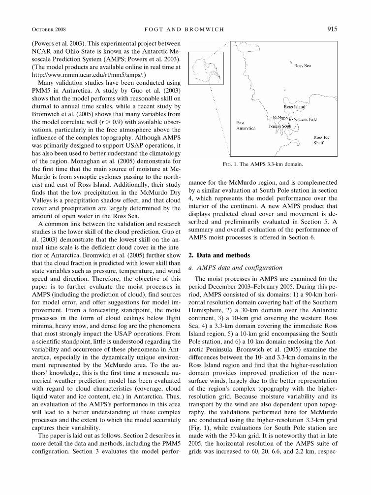
Here, the AWEX-corrected relative humidity mea-surements from the McMurdo radiosonde record arecompared to AMPS predictions at most mandatory lev-els up to 100 hPa. Figure 2 displays the relative humid-ity with respect to ice (rhice) correlation (Fig. 2a) andbias (model minus observations; Fig. 2b). The statisticshere provide insight beyond that of Bromwich et al.(2005) as they consider levels above 500 hPa and below850 hPa, observations that are corrected for measure-ment error, and are separated for various forecasthours. Interestingly, Fig. 2 demonstrates a peak in the


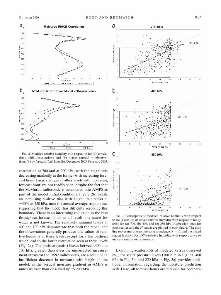
correlation at 700 and at 200 hPa, with the magnitudedecreasing markedly at the former with increasing fore-cast hour. Large changes at other levels with increasingforecast hour are not readily seen, despite the fact thatthe McMurdo radiosonde is assimilated into AMPS aspart of the model initial conditions. Figure 2b revealsan increasing positive bias with height that peaks at�40% at 250 hPa, near the annual average tropopause,suggesting that the model has difficulty resolving thisboundary. There is an interesting reduction in the biasthroughout forecast hour at all levels, the cause forwhich is not known. The relatively minimal biases at400 and 100 hPa demonstrate that both the model andthe observations generally produce low values of rela-tive humidity at these levels, except for a few outliers,which lead to the lower correlation seen at these levels(Fig. 2a). The positive (moist) biases between 400 and100 hPa, greater than even the uncorrected measure-ment errors for the RS92 radiosondes, are a result of aninsufficient decrease in moisture with height in themodel, as the vertical moisture gradient in AMPS ismuch weaker than observed up to 200 hPa.

Examining scatterplots of modeled versus observedrhice for select pressure levels (700 hPa in Fig. 3a, 400hPa in Fig. 3b, and 250 hPa in Fig. 3c) provides addi-tional information regarding the moisture predictionskill. Here, all forecast hours are retained for compari-

FIG. 2. Modeled relative humidity with respect to ice (a) correla-tions with observations and (b) biases (model � observa-tions, %) by forecast (fcst) hour (h), December 2003–February 2005.

FIG. 3. Scatterplots of modeled relative humidity with respectto ice (x axis) vs observed relative humidity with respect to ice (yaxis) for (a) 700, (b) 400, and (c) 250 hPa. Regression lines foreach scatter and the r2 values are plotted in each figure. The grayline represents one-to-one correspondence (x � y), and the boxedregion is drawn for 100% relative humidity with respect to ice toindicate saturation occurrence.


son; thus, during the summer, two forecasts are com-pared to the 1200 UTC data (the 12- and 36-h fore-casts). All months are also retained as the seasonalchanges in relative humidity correlation and bias arerelatively small (not shown), in agreement with Brom-wich et al. (2005) who similarly find little interseasonalvariation in model skill for many of the state variables(i.e., temperature, pressure). The scatterplots in Fig. 3also have a one-to-one line that helps to display biases,as positive (negative) biases fall below (above) this line.A regression line and the r2 value are also plotted foreach figure to examine the correlation and persistentbiases, while values outside of the rectangles in Fig. 3indicate saturation with respect to ice (hereafter satice),an important characteristic for cloud formation.

As expected from Fig. 2, the scatterplots demonstratethe best overall skill at 700 hPa (Fig. 3a), where theregression line is very similar to the one-to-one line andthe r2 value is the highest. At 700 hPa, satice is alsopredicted well, and at comparable frequencies in boththe model and observations. The r2 value is lowest at400 hPa (Fig. 3b), clearly generated by the large spreadof the observed rhice values at all modeled rhice values.In contrast to this, the observed rhice values are oftenvery small while the model has a much greater range inrhice values at 250 hPa (Fig. 3c). However, at 400 and250 hPa, AMPS predicts rhice �100% much more fre-quently than observed, and for a much greater range ofobserved rhice values.

b. Cloud fraction

In AMPS, CF is calculated from AMPS model out-put, based on the integrated cloud optical depth, �,adapted from the Community Climate Model, version 2(CCM2), radiation scheme that is employed by PMM5(Hack et al. 1993):

CF � � � �sfc

toa

0.1CLWP � 0.0735CIWP, 1

where CLWP is the cloud liquid water path and CIWPis the cloud ice water path at each 1⁄2 sigma level, and sfcindicates the surface and toa indicates the top of theatmosphere (50 hPa in AMPS). The CLWP and CIWPare in grams per square meter, and are based on themicrophysical quantities of cloud liquid water and iceconcentrations (CLW and CICE, respectively; g kg�1),as given in Eqs. (2) and (3):

CLWP � � p

T � 287�� CLW � dz and 2

CIWP � � p

T � 287�� CICE � dz, 3

where p is the pressure (Pa) and T is the temperature(K) at each 1⁄2 sigma level, and dz is the change inheight (m) between the 1⁄2 and full sigma levels, whichaccounts for forecast pressure changes. Cassano et al.(2001) provide further details regarding how the CLWPand CIWP are determined in PMM5. The constants0.1 m2 g�1 and 0.0735 m2 g�1 in Eq. (1) are longwaveabsorption coefficients, but were derived for midlati-tude conditions as part of the CCM2 radiation scheme.The CF is restricted to be less than or equal to 1.

Values for the CF extracted for the model grid pointsrepresenting each of the locations in Fig. 1 are com-pared with observations to better understand the cloudvariability within AMPS. The CF error distribution(model � observations) is displayed in Fig. 4a for thesummer seasons when measurements are routinelytaken at all three locations, and Fig. 4b for all seasons atMcMurdo; Table 1 lists the statistical characteristics ofthe distributions presented in Fig. 4. Notably, the per-formance at all three stations in summer is very similar,despite the fact that McMurdo is protected from thefrequent southerly winds over the Ross Ice Shelf that

FIG. 4. Cloud fraction difference (model � observations) dis-tributions for (a) Williams Field, Pegasus Field, and McMurdo forsummer and (b) McMurdo only, but by season.


often bring cloud and snow to Pegasus and WilliamsFields (cf. Fig. 10 of Bromwich et al. 2005). However,Fig. 4a and Table 1 shows that the model often under-predicts cloudiness throughout the year (largest duringthe warmer months) as determined by the CF, in agree-ment with previous studies (Guo et al. 2003; Bromwichet al. 2005). However, this study disagrees with Guo etal. (2003), who relate this negative CF bias to a low-level dry bias, since our relative humidity comparisonsindicate that AMPS has excessive rhice throughout thetroposphere (Fig. 2b), albeit small positive biases closerto the surface. The correlation with the observations isslightly lower than the relative humidity correlations(cf. Table 1 and Fig. 2), but is in agreement with Brom-wich et al. (2005).

To improve the relationship between observed andmodeled CF, several combinations of the coefficientsfor CLWP and CIWP in Eq. (1) (which were developedfor midlatitude conditions) were tested to produce thedistribution that best aligns with the observations andremoves the negative bias (underprediction of clouds).In this process it was found that the coefficients 0.075m2 g�1 for the CLWP and 0.170 m2 g�1 for the CIWPare the most optimal, where more than twice as muchweight was given to the CIWP. Lubin (1994) finds thatthe emissivity of maritime Antarctic clouds is smallerthan the CLWP used in the NCAR Community Cli-mate Model 1, and therefore finds that a better absorp-tion coefficient for CLWP was 0.065 m2 g�1, very simi-lar to the 0.075 m2 g�1 CLWP determined here.

Notably, Lachlan-Cope et al. (2001) find more icecrystals present in clouds over the Avery Plateau on theAntarctic Peninsula than expected in the midlatitudes,confirming that more weight needs to be given to theCIWP for Antarctic clouds. Their study also found su-percooled liquid water in the clouds they observed,while tethered cameras flown into clouds at the South

Pole station, representative of the interior of the con-tinent, have also noted the presence of supercooled liq-uid water primarily during December and January andrarely during October–November and February–March (M. Town 2006, personal communication). To-gether, these limited studies suggest ice particles domi-nate Antarctic cloudiness but that supercooled liquidwater is indeed present, especially during the warmersummer months; thus, at least some weight must begiven to the CLWP in the CF algorithm.

Despite the fact that little is known on cloud vari-ability in Antarctica, applying more weight to theCIWP substantially increases the ability for AMPS toaccurately predict the CF amount, as indicated in Fig. 5and the right columns of Table 1. The modified algo-rithm produces a near-zero bias in all seasons exceptwinter (which a Student’s t test indicates is statisticallydifferent from the previous distribution at p � 0.01),and reduces the underprediction of clouds by as muchas 5% on average at all sites. The modified CF algo-rithm also produces a better alignment with high valuesof relative humidity within the model and the overcastcloud layers (not shown), with improvements from theoriginal to the modified algorithm leading to changes ofas much as 20%. However, given that the CF correla-tion does not change using the new algorithm suggeststhat AMPS is accurately predicting CICE variability,but not producing enough CLW variability to matchwith the observed CF (and therefore produce a highercorrelation). This conjecture will be examined in sec-tion 5.

4. AMPS validation at South Pole station

As the performance at McMurdo extends to othercoastal stations (Bromwich et al. 2005), we now exam-

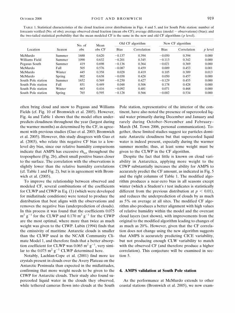
TABLE 1. Statistical characteristics of the cloud fraction error distributions in Figs. 4 and 5, and for South Pole station: number offorecasts verified (No. of obs); average observed cloud fraction (mean obs CF); average difference (model � observations) (bias); andthe two-tailed statistical probability that the mean modeled CF is the same in the new and old CF algorithms (p level).

Location SeasonNo. of

obsMean

obs CF

Old CF algorithm New CF algorithm

p levelBias Correlation Bias Correlation

McMurdo Summer 1688 0.620 �0.137 0.394 �0.050 0.394 0.000Williams Field Summer 1090 0.632 �0.201 0.345 �0.113 0.342 0.000Pegasus South Summer 419 0.698 �0.136 0.364 �0.021 0.369 0.000McMurdo Fall 505 0.576 �0.087 0.459 0.009 0.453 0.001McMurdo Winter 445 0.358 0.028 0.419 0.105 0.389 0.013McMurdo Spring 802 0.638 �0.038 0.428 0.050 0.457 0.000South Pole station Summer 1652 0.569 �0.250 0.427 �0.129 0.455 0.000South Pole station Fall 851 0.449 0.048 0.506 0.178 0.428 0.000South Pole station Winter 663 0.416 �0.092 0.481 0.071 0.468 0.000South Pole station Spring 765 0.595 �0.128 0.566 �0.002 0.534 0.000


ine the performance over the interior of the continentby employing observations from the South Pole stationcompared with AMPS data from the 30-km grid, theonly domain covering the region available in the AMPSarchive. South Pole station was chosen as it was theonly interior station to have radiosonde launches con-tinuously throughout the year, which allows for exami-nation of the relative humidity performance and cloudcover as was conducted for McMurdo.

a. Relative humidity

The relative humidity evaluations at South Pole sta-tion are presented in Fig. 6. Here, the AMPS rhice cor-relation with observations (Fig. 6a) ranges between 0.3and 0.5 throughout much of the troposphere, slightlylower than that at McMurdo (Fig. 2a). The better per-formance above 250 hPa is due to the reduced moisturevariability in the upper troposphere–lower stratosphereover the continental interior, which is adequately de-picted in AMPS despite the fact that the correlationdrops notably at these levels with increasing forecasthour. Below 250 hPa, the 24-, 48-, and 72-h forecastsshow similar (and higher) skill as only these forecastsalign with the 0000 UTC soundings taken during the offseason. The lower skill at the other forecast hours ismost likely tied to increased moisture variability in thelower troposphere during the summer at South Polestation, which is not captured as well in AMPS. Thebiases (Fig. 6b) are �10% larger than at McMurdo(Fig. 2b), and also increase with height to �50% at 250hPa, which is also near the tropopause. As at Mc-Murdo, this increasing bias with height is related to aninaccurate vertical depletion of moisture that also existsover the continental interior in AMPS. Interestingly,the biases again decrease with increasing forecast hour,for uncertain reasons.

b. Cloud fraction

Before CF comparisons can be made, some com-ments must first be made about the observed cloudcover at South Pole station, a much different environ-ment than McMurdo. Many problems complicate theground-based visual cloud cover observations at SouthPole station, including the very thin nature of clouds atall levels through which the sun/stars are often seen[these conditions tend to favor partly cloud observa-tions instead of overcast conditions; Mahesh et al.(2001); Bernhard et al. (2004); Town et al. (2007)], a6-month period of complete darkness, making cloudsdifficult to observe, and extremely cold temperaturesyear round with especially strong inversion layers in thewinter (Turner and Pendlebury 2007). Town et al.(2005) further note the persistent presence of “diamonddust” or clear-sky precipitation during the winter,which may also add to errors in observed cloud fraction.They note that the wintertime average cloud fractionobtained from spectral infrared data is 0.3–0.5 greaterthan that obtained from visual observations. Therefore,the agreement between modeled and observed cloudsshould not align as well as at McMurdo, especially dur-ing the nondaylight hours.

FIG. 5. As in Fig. 4a but for the modified CF algorithm (solid).The dashed lines are the values from the original CF algorithm(Fig. 4a).

FIG. 6. As in Fig. 2 but for South Pole station.


Seasonal CF statistics are presented for the originaland the modified CF algorithms in the bottom rows ofTable 1. Clouds are also underpredicted in AMPS usingthe original CF algorithm at South Pole station, and themean bias is �0.135 for the time period considered.Notably, there is a much more marked seasonal cycle atSouth Pole station; the bias during austral fall is smalland positive (0.048), while the bias is much farther fromzero during the summer (�0.250). However, the posi-tive bias in fall may be related to a known negative biasin observed CF compared against independent data(Town et al. 2007). Incorporating the modified CF al-gorithm again substantially reduces the mean bias to�0.004, effectively centering the error distribution overzero, with these changes being highly statistically sig-nificant (p � 0.001; Table 1). The exception is for fall,where a larger positive bias is introduced by switchingfrom the original to the modified CF algorithm; the biasusing the modified CF algorithm also becomes positiveduring winter, but both of these seasons are markedwith a negative bias in observed cloud cover (Town etal. 2007), so AMPS is likely predicting reliable CFamounts in these seasons. During the other seasons, thebiases improve by �0.12 and are closer to zero thanwhen using the previous CF values. This further dem-onstrates that adjustments to the coefficients in the em-pirical CF algorithm can reduce the bias not only in theMcMurdo region, but over the entire Antarctic conti-nent. However, the fact that the correlation againchanges little with the new CF algorithm suggestschanges in the model physics, and particularly in thecalculation of CLW (given that the changes in the CFalgorithm are primarily tied to large changes in theweight given to CICE), are needed to improve the pre-diction of CF temporal variability.

Finally, the cloud prediction performance at SouthPole station is evaluated by forecast hour for varioussky coverage criteria (overcast, CF � 0.8; partly cloudy,0.2 � CF � 0.8; and clear, CF � 0.2). To facilitateinterpretation, only the percentage of matched fore-casts (both the model and the observation indicate thesame sky coverage) with respect to the total number ofobservations is plotted against forecast hour (Fig. 7).The modified CF greatly improves the number ofmatched forecasts of the overcast conditions by asmuch as 20%, with only slight decreases in the numberof matches for clear and partly cloudy conditions forthe early to midforecast hours. However, these changesare much smaller than the large improvements gainedin the prediction of overcast conditions, which have themost impact on aircraft operations. Additionally, othertests (not shown) demonstrate that the model rarelypredicts CF that falls in the partly cloudy range, but

rather tends to predict overcast and clear conditionsinstead, in agreement with the known U distribution ofobserved cloud cover at South Pole station (Town et al.2007). Thus, the forecast skill is the lowest for the partlycloudy sky coverage regardless of the empirical algo-rithm employed. In contrast to other fields, Fig. 7 showsthat overall the model skill for cloud prediction doesnot vary substantially between forecast hours, althoughthere appears to be some slight degradation in time forovercast and partly cloudy conditions, especially thelatter using the original algorithm. A possible explana-tion for why fewer changes with forecast hour are seenin the cloud predictions (Fig. 7) compared to the rela-tive humidity predictions (Figs. 2 and 6) is that relativehumidity observations are assimilated into the initialconditions in AMPS, while clouds are generated by themodel physics. Bromwich et al. (1999) note that thedistinction between coastal and interior moisture con-ditions lessens with forecast time in older versions ofthe National Centers for Environmental Prediction(NCEP) operational Global Spectral Model. Notably,NCEP’s Aviation Model (AVN) supplies the initial andboundary conditions for AMPS, so the problems ob-served in Bromwich et al. (1999) may still affect thecurrent AMPS forecasts.

5. The pseudosatellite product

The previous validation tests have reached an impor-tant conclusion regarding the cloud variability inAMPS: changes to the coefficients of CLWP and CIWPin Eq. (1) produce a CF that has near-zero bias withobservations, while the microphysics scheme appears tonot produce enough CLW, leading to the low CF cor-relation. Although AMPS has a strong positive mois-ture bias near the tropopause, the model relative hu-midity values infrequently achieve saturation with re-

FIG. 7. Percent matches for South Pole station by forecast hourgrouped by various sky conditions. Time series with markers in-dicate matches from the new cloud fraction algorithm.


spect to ice (cf. Fig. 3c), which suggests that the positivemoisture biases are not influencing the CF bias. Fur-ther, Antarctic clouds rarely form as high as the tropo-pause (e.g., Mahesh et al. 2001), and high cloud condi-tions are classified starting at 11 000 ft (�600 hPa)above mean sea level (Turner and Pendlebury 2007).To assess the model performance further, it is necessaryto examine a more complete visualization of the cloudcharacteristics, such as in satellite imagery, as CF onlydetails cloud coverage at a single point and not thespatial variability of cloud height, thickness, or layers.Visualizations that display all these cloud featureswould also be very beneficial operationally, as Antarc-tic forecasters rely heavily on available satellite imagery(cloud characteristics) to track the timing and coverageof cloud layers and their associated precipitation (ifany) due to the lack of observations of these fields.

To aid in this regard, the Polar Meteorology Groupof the Byrd Polar Research Center recently developedand initially tested a “pseudosatellite” product. Thisproduct, now available in real time as a standard fore-cast product from AMPS (see online at http://box.mmm.ucar.edu/rt/mm5/amps/), uses the vertically inte-grated CLW and CICE species from AMPS [see Eqs.

(2) and (3)] to generate a pseudosatellite image thatroughly follows the Antarctic infrared color compositesgenerated by the AMRC. [Vukicevic et al. (2004) de-scribe a similar product based on cloud mixing ratio.]The product improves upon the CF and cloud-baseproducts in AMPS as it separates low clouds, displayedwith blue to gray shades in the product, specified fromthe vertical integral of the CLW species, from higherclouds (white shades) depicted from the vertical inte-gral of the CICE. The pseudosatellite was first availablein late 2005, and was used by forecasters during the2005–06 and 2006–07 field seasons as it successfully pro-vided additional guidance on cloud movement and as-sociated precipitation.

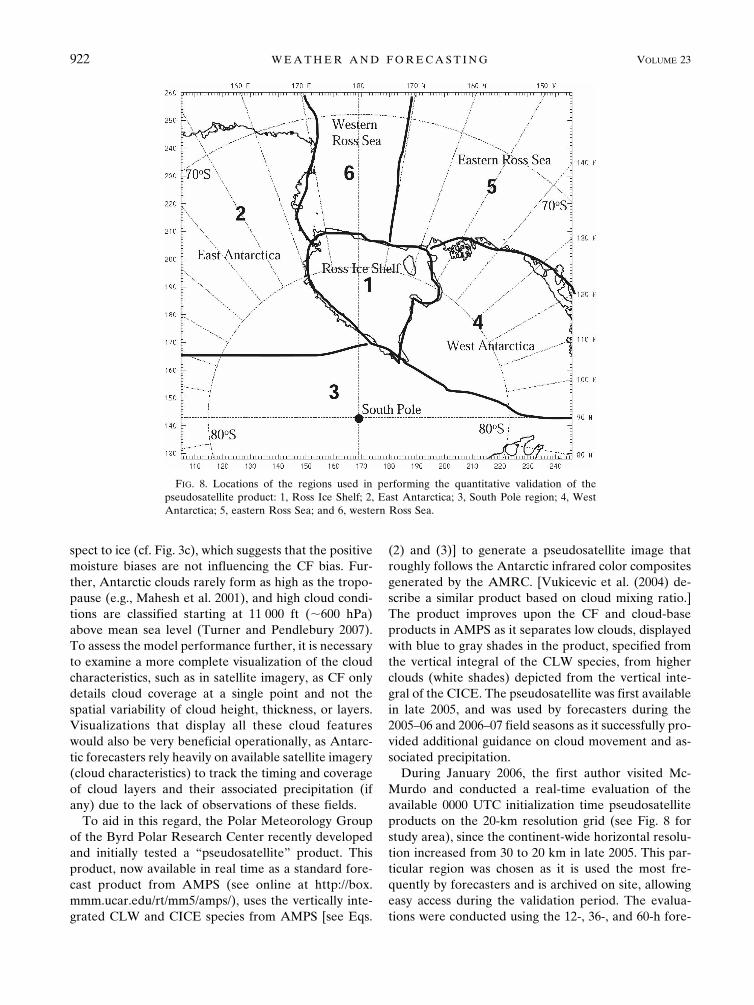
During January 2006, the first author visited Mc-Murdo and conducted a real-time evaluation of theavailable 0000 UTC initialization time pseudosatelliteproducts on the 20-km resolution grid (see Fig. 8 forstudy area), since the continent-wide horizontal resolu-tion increased from 30 to 20 km in late 2005. This par-ticular region was chosen as it is used the most fre-quently by forecasters and is archived on site, allowingeasy access during the validation period. The evalua-tions were conducted using the 12-, 36-, and 60-h fore-

FIG. 8. Locations of the regions used in performing the quantitative validation of thepseudosatellite product: 1, Ross Ice Shelf; 2, East Antarctica; 3, South Pole region; 4, WestAntarctica; 5, eastern Ross Sea; and 6, western Ross Sea.


casts initialized from 12 to 24 January 2006 for a total of35 forecasts (missing the 60-h forecast from 24 Janu-ary). Only these forecast hours were used since theyrepresent the most spatially complete concurrent De-fense Meteorological Satellite Program (DMSP) ther-mal infrared satellite image (�0.5 km resolution), withwhich the pseudosatellite forecasts were compared todetermine the skill in the cloud placement (coverageand location) and movement (timing and temporalchanges in coverage). The validations were also madeby regions (Fig. 8) that together cover many more dif-ferent synoptic environments than were previouslyevaluated at South Pole station and McMurdo. Ob-served cloud heights in the imagery are determined bytheir contrast to the surface, and because middle cloudsare not easily identified in these satellite images or inthe pseudosatellite product, a comparison of this cloudtype is not conducted explicitly here. However, it ispossible that human error may lead to the incorrectcategorization of any cloud level, and not just themidlevel clouds. Although the validation period is rela-tively short, it contains a diversity of weather features,suggesting that additional comparisons will yield similarresults. We constructed 2 � 2 contingency tables, alongwith their associated verification statistics [see Murphy(1996) and Wilks (2006) for a detailed description ofthese statistics], for each region in Fig. 8 as a means of

quantitatively evaluating the pseudosatellite product,separated by low clouds (Table 2) and high clouds(Table 3). Matched (clouds–clouds or clear–clear) fore-casts were recorded when both the model and satelliteimagery displayed nearly the same cloud cover in thesame location for each region.

For low clouds (Table 2), the percent correct is oftenless than 50% for all regions, except for East Antarcticawhere AMPS accurately predicts the infrequent low-level cloudiness. Over the continent, the biases are allless than 0.3, suggesting a strong underprediction of lowclouds, while there is an overprediction of clouds in thewestern Ross Sea. The various skill scores, with theexception of the eastern Ross Sea, are weakly positive,suggesting a slight skill above random forecasts, whilethe negative skill scores in the eastern Ross Sea implythat the model prediction of low cloudiness in this re-gion is less than would be obtained by chance, governedby the 1.0 false alarm ratio (i.e., the inability to accu-rately predict clear conditions in the region). This as-sessment of the low clouds is in direct agreement withthe conjecture that the model has difficulty in predict-ing the CLW variability, which leads to low a CF cor-relation with the observations.

Turning to the high cloud verification (Table 3), agreater level of skill is attained with the percent correctbeing above 80% in the majority of the regions, biases

TABLE 2. The 2 � 2 contingency tables and associated statistical skill scores as described in Murphy (1996) and Wilks (2006) for thelow cloud performance of the pseudosatellite product for the regions defined in Fig. 8. To be counted as a match (i.e., clouds–cloudsor clear–clear), the CLW content in the pseudosatellite product must closely match the coverage in the concurrent satellite imagery.Using the schematic, the chi-squared probability is the statistical probability that a, b, c, and d are independent; percent correct �(a � d)/n, where n is the total observations (35 here); threat score � a/(a � b � c); bias � (a � b)/(a � c); false alarm ratio �b/(a � b); false alarm � b/(b � d); hit rate � a/(a � c); HSS is the Heidke skill score; PSS is the Peirce skill score; CSS is the Claytonskill score; and GSS is the Gilbert skill score. HSS, PSS, and CSS all range from �1 to 1, with 1 indicating perfect forecast skill, 0indicating random forecast performance, and �1 indicating the worst possible skill; the GSS ranges from 0 to 1, with 1 indicating perfectforecast skill.

Schematic

AMPS

Obs

Yes No Ross Ice Shelf East Antarctica South Pole region West Antarctica Eastern Ross Sea Western Ross Sea

Yes a b 7 0 3 0 3 0 3 0 17 10 12 15

No c d 22 6 8 24 12 20 26 6 8 0 3 5

Chi-squaredprobability

0.18 0.01 0.04 0.41 0.04 0.73

Percent correct 37.14 77.14 65.71 25.71 48.57 48.57Threat score 0.24 0.27 0.20 0.10 0.49 0.40Bias 0.24 0.27 0.20 0.10 1.08 1.80False alarm ratio 0.00 0.00 0.00 0.00 0.37 0.56False alarm 0.00 0.00 0.00 0.00 1.00 0.80Hit rate 0.24 0.27 0.20 0.10 0.68 0.75HSS 0.10 0.34 0.22 0.04 �0.34 0.05PSS 0.24 0.27 0.20 0.10 �0.32 0.05CSS 0.21 0.75 0.63 0.19 �0.37 0.07GSS 0.06 0.03 0.02 0.01 0.48 0.40


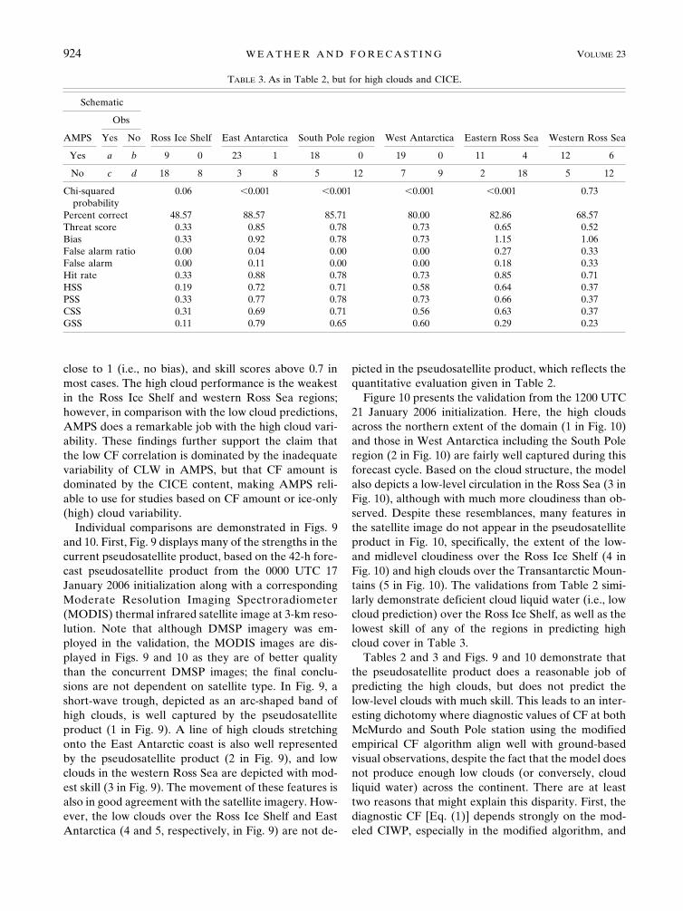
close to 1 (i.e., no bias), and skill scores above 0.7 inmost cases. The high cloud performance is the weakestin the Ross Ice Shelf and western Ross Sea regions;however, in comparison with the low cloud predictions,AMPS does a remarkable job with the high cloud vari-ability. These findings further support the claim thatthe low CF correlation is dominated by the inadequatevariability of CLW in AMPS, but that CF amount isdominated by the CICE content, making AMPS reli-able to use for studies based on CF amount or ice-only(high) cloud variability.

Individual comparisons are demonstrated in Figs. 9and 10. First, Fig. 9 displays many of the strengths in thecurrent pseudosatellite product, based on the 42-h fore-cast pseudosatellite product from the 0000 UTC 17January 2006 initialization along with a correspondingModerate Resolution Imaging Spectroradiometer(MODIS) thermal infrared satellite image at 3-km reso-lution. Note that although DMSP imagery was em-ployed in the validation, the MODIS images are dis-played in Figs. 9 and 10 as they are of better qualitythan the concurrent DMSP images; the final conclu-sions are not dependent on satellite type. In Fig. 9, ashort-wave trough, depicted as an arc-shaped band ofhigh clouds, is well captured by the pseudosatelliteproduct (1 in Fig. 9). A line of high clouds stretchingonto the East Antarctic coast is also well representedby the pseudosatellite product (2 in Fig. 9), and lowclouds in the western Ross Sea are depicted with mod-est skill (3 in Fig. 9). The movement of these features isalso in good agreement with the satellite imagery. How-ever, the low clouds over the Ross Ice Shelf and EastAntarctica (4 and 5, respectively, in Fig. 9) are not de-

picted in the pseudosatellite product, which reflects thequantitative evaluation given in Table 2.

Figure 10 presents the validation from the 1200 UTC21 January 2006 initialization. Here, the high cloudsacross the northern extent of the domain (1 in Fig. 10)and those in West Antarctica including the South Poleregion (2 in Fig. 10) are fairly well captured during thisforecast cycle. Based on the cloud structure, the modelalso depicts a low-level circulation in the Ross Sea (3 inFig. 10), although with much more cloudiness than ob-served. Despite these resemblances, many features inthe satellite image do not appear in the pseudosatelliteproduct in Fig. 10, specifically, the extent of the low-and midlevel cloudiness over the Ross Ice Shelf (4 inFig. 10) and high clouds over the Transantarctic Moun-tains (5 in Fig. 10). The validations from Table 2 simi-larly demonstrate deficient cloud liquid water (i.e., lowcloud prediction) over the Ross Ice Shelf, as well as thelowest skill of any of the regions in predicting highcloud cover in Table 3.

Tables 2 and 3 and Figs. 9 and 10 demonstrate thatthe pseudosatellite product does a reasonable job ofpredicting the high clouds, but does not predict thelow-level clouds with much skill. This leads to an inter-esting dichotomy where diagnostic values of CF at bothMcMurdo and South Pole station using the modifiedempirical CF algorithm align well with ground-basedvisual observations, despite the fact that the model doesnot produce enough low clouds (or conversely, cloudliquid water) across the continent. There are at leasttwo reasons that might explain this disparity. First, thediagnostic CF [Eq. (1)] depends strongly on the mod-eled CIWP, especially in the modified algorithm, and

TABLE 3. As in Table 2, but for high clouds and CICE.

Schematic

AMPS

Obs

Yes No Ross Ice Shelf East Antarctica South Pole region West Antarctica Eastern Ross Sea Western Ross Sea

Yes a b 9 0 23 1 18 0 19 0 11 4 12 6

No c d 18 8 3 8 5 12 7 9 2 18 5 12

Chi-squaredprobability

0.06 �0.001 �0.001 �0.001 �0.001 0.73

Percent correct 48.57 88.57 85.71 80.00 82.86 68.57Threat score 0.33 0.85 0.78 0.73 0.65 0.52Bias 0.33 0.92 0.78 0.73 1.15 1.06False alarm ratio 0.00 0.04 0.00 0.00 0.27 0.33False alarm 0.00 0.11 0.00 0.00 0.18 0.33Hit rate 0.33 0.88 0.78 0.73 0.85 0.71HSS 0.19 0.72 0.71 0.58 0.64 0.37PSS 0.33 0.77 0.78 0.73 0.66 0.37CSS 0.31 0.69 0.71 0.56 0.63 0.37GSS 0.11 0.79 0.65 0.60 0.29 0.23


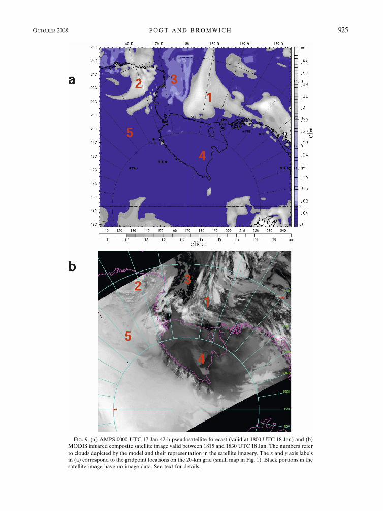
FIG. 9. (a) AMPS 0000 UTC 17 Jan 42-h pseudosatellite forecast (valid at 1800 UTC 18 Jan) and (b)MODIS infrared composite satellite image valid between 1815 and 1830 UTC 18 Jan. The numbers referto clouds depicted by the model and their representation in the satellite imagery. The x and y axis labelsin (a) correspond to the gridpoint locations on the 20-km grid (small map in Fig. 1). Black portions in thesatellite image have no image data. See text for details.


Fig 9 live 4/C

FIG. 10. (a) AMPS 12 UTC 21 Jan 45-h pseudosatellite forecast (valid at 0900 UTC 23 Jan) and (b)MODIS infrared satellite composite image valid between 0915 and 0920 UTC 23 Jan. The numbers referto clouds depicted by the model and their representation in the satellite imagery. The x and y axis labelsin (a) correspond to the gridpoint locations on the 20-km grid (small map in Fig. 1). Black portions in thesatellite image have no image data. See text for details.


Fig 10 live 4/C

not the CLWP. Therefore, deficient CLW does not nec-essarily lead to low modeled CF. Second, cloud cover(height and fraction) observations at McMurdo indicatethat high clouds play a dominating role in the total CF

amount, as cloud ceilings are reported at mid- and high(ice clouds in the pseudosatellite product) levels morethan 50% of the time, and the remaining percentage oflow cloud ceilings may often have high cloud cover not

FIG. 11. Mean summer (Dec 2003–Feb 2004 and Dec 2004–Feb 2005) vertically integrated(a) cloud ice and (b) cloud liquid water, given that the 2-m relative humidity with respect towater is �80%. Contour interval is 0.005 mm in (a) and 0.01 mm in (b) above 0.01 mm, withthe 0.0025-mm level thickened for reference in (b).


seen by manual observations. These combined effectssuggest that although deficient model physics (shortageof cloud liquid water) clearly play a role in the under-prediction of cloud seen in the original CF algorithm(and especially CF variability/correlation), the domi-nance of high clouds in determining the CF amount andthe good prediction of these clouds by AMPS demon-strates that AMPS produces sufficient CICE. This con-sequently leads to an overall good agreement betweenthe observed and modeled CFs in the modified algo-rithm, regardless of the presence or accuracy of thelow-level cloudiness prediction.

Nonetheless, it is interesting that the small skill oflow-level cloud prediction in the pseudosatellite prod-uct, and brings doubt upon the reliability of the micro-physics scheme in AMPS in producing mixed-phaseclouds. To understand this deficiency, Fig. 11 displaysthe summer average (averaged over the two summerseasons of 2003/04 and 2004/05) vertically integratedCICE (Fig. 11a) and CLW (Fig. 11b) in AMPS, themodel variables upon which the pseudosatellite productis based. The averages are only calculated for caseswhen the 2-m relative humidity with respect to water isgreater than or equal to 80% in order to provide abetter estimate on the magnitude of these cloud micro-physical quantities during cloudy conditions within themodel. Independent tests (not shown) determine thatclouds are present in satellite imagery based on thiscriterion more than 85% of the time except in the RossIce Shelf and West Antarctica regions, where the asso-ciation drops to 75%. Figure 11a demonstrates smallconcentrations of cloud ice over much of Antarctica, inagreement with known climatologies (e.g., Stone 1993),with the highest values of cloud ice found along thecoast and the Antarctic Peninsula. Meanwhile, it is ap-parent that AMPS does not produce much cloud liquidwater over the interior of the continent, as the 0.025contour roughly follows the coast of Antarctica in Fig.11b, and only extends to higher latitudes over the iceshelves and coastal West Antarctica. Despite the factthat summer near-surface temperatures can be warmerthan �34°C within the 0.025-mm contour in Fig. 11b,the coldest temperature at which Beesley et al. (2000)demonstrated the presence of supercooled liquid waterin the Arctic, AMPS rarely produces any liquid waterover the interior of the continent. Morrison et al. (2003)demonstrate a similar problem in modeling the CLW ina single-column model in the Arctic. Compared withdata from the Surface Heat Budget of the Arctic(SHEBA) project, they noted an underestimation ofthe CLW by 42%, which was found to be sensitive tothe ice crystal concentration. Other recent modelingstudies in the Arctic compared with SHEBA data note

similar deficiencies in modeling supercooled liquid wa-ter using the Reisner et al. (1998) scheme that is cur-rently used in AMPS (Morrison and Pinto 2005, 2006;Morrison et al. 2005). Consequently, Morrison andPinto (2006) find that a scheme that not only predictsmixing ratios of the hydrometeor species of cloud ice,cloud liquid water, rain, and snow within cloud layers[as in the Reisner et al. (1998) scheme], but also thenumber concentration of these species, is required togenerate sufficient supercooled liquid water that is inbetter agreement with the observations. These studieshelp to explain the deficiency in low-cloud predictionby the pseudosatellite product as well as what changesare needed to predict the CLW variability and, there-fore, likely improve the CF correlation.

6. Summary and conclusions

This paper has provided a detailed evaluation of theAMPS forecast atmospheric moisture and cloud char-acteristics. At both McMurdo and South Pole station,AMPS displays a positive relative humidity bias thatincreases with height up to 250–200 hPa, related to aweaker vertical decrease of moisture in AMPS com-pared with the observations. The bias is reduced at 100hPa, where both the model and observations have verylow values of relative humidity. The correlation withthe observations is greatest at McMurdo in the lowertroposphere where more moisture is available, andgreater at South Pole station in the upper troposphereto lower stratosphere, where both the model and ob-servations show reduced variability in atmosphericmoisture.

Cloud prediction by AMPS was evaluated using ob-servations of CF at McMurdo and South Pole stationand by comparing the pseudosatellite product, based onthe microphysical quantities of cloud liquid water andcloud ice, with DMSP imagery. After adjusting the em-pirical CF algorithm to give more than twice as muchweight to the CIWP, the CF error distribution is ap-proximately centered on zero for both McMurdo andSouth Pole station, although the correlation is not im-proved and remains �0.4. Nonetheless, the modifiedCF algorithm produces overcast conditions that betteralign with observations throughout all forecast hours atboth sites. Validations of the pseudosatellite productdemonstrate good skill in predicting high cloud cover.As high clouds are shown to dominate the total CFamount, they help to explain the strong agreement be-tween the modeled and observed CF amounts. How-ever, it was found that the microphysics scheme doesnot produce enough CLW over the interior of the con-tinent, and that improvements in the variability of


CLW in the microphysics scheme are needed to im-prove the CF correlation and prediction of low cloudsin the pseudosatellite product. Notably, the accurateCICE variability and amount appears unrelated to theexcessive model relative humidity near the tropopause,as even with these positive biases the model infre-quently produces saturation with respect to ice above500 hPa (cf. Fig. 3c).

Nonetheless, it is apparent that the skill of cloudcharacteristics predicted by AMPS exceeds that ofother similar atmospheric models. Hinkelman et al.(1999) find that the Eta Model has more inaccuratelypredicted clouds than correctly predicted clouds (basedprimarily on cloud height), as evaluated with observa-tions at the Atmospheric Radiation Measurement(ARM) site in Oklahoma. In the Arctic, the greatestdisagreement between eight different regional climatemodels was found in the predicted cloud cover, whichled to errors in the surface radiation fluxes and 2-mtemperature (Rinke et al. 2006) as evaluated with datafrom the SHEBA project. Hines et al. (2004) find simi-lar errors in predicting Antarctic clouds within theNCAR climate models, especially noting that theclouds over the interior of the continent are too opti-cally thick. Their study found that allowing for greaterquantities of precipitate to fall out of the clouds pro-duced better agreement between the observed winter-time temperatures and the downwelling shortwave ra-diation during summer. However, the validations pre-sented here indicate that the cloud prediction by AMPSshows superior skill to these models, given that the tem-perature fields in AMPS are in good agreement withavailable observations (Bromwich et al. 2005), adjust-ments to the empirical CF algorithm produces near-zero bias at both McMurdo and South Pole station, andhigh cloud variability is captured well within the regionand time period studied.

Future plans include a much more extensive evalua-tion of the pseudosatellite’s performance, including thedevelopment of a product that uses the relative humid-ity fields to display modeled clouds, as well as furthertesting of AMPS cloud prediction performance usingdownwelling radiation measurements. Despite theknown deficiencies, the pseudosatellite product cur-rently serves as an important and powerful forecastingtool, as well as a potential research tool to better un-derstand the climatology of clouds in an observationallysparse region. Given the high skill of the AMPS systemdisplayed here with the modified CF algorithm and inhigh cloud prediction, it is likely that additional re-search that considers CF amount, high cloud variability,and moist processes in general can be conducted usingAMPS. As such, model evaluations such as the one

presented here not only serve the Antarctic forecastingcommunity and AMPS users, but also the larger scien-tific community that uses AMPS archived forecasts toconduct climate studies across the Antarctic continent.

Acknowledgments. The authors thank Kathie Hilland Michael Town for discussions regarding cloud vari-ability and observations at South Pole station, DanielSteinhoff for processing and obtaining the satellite im-agery for Figs. 9 and 10 from NASA’s Level 1 Atmo-spheric Archive and Distribution System, and NSF forsupporting the site visit by RLF to McMurdo and SouthPole station in January 2006. This research was fundedby UCAR Subcontract SO1-22961 and NSF GrantOPP-0337948.

REFERENCES

Beesley, J. A., C. S. Bretherton, C. Jakob, E. L. Andreas, J. M.Intrieri, and T. A. Uttal, 2000: A comparison of cloud andboundary layer variables in the ECMWF forecast model withobservations at Surface Heat Budget of the Arctic Ocean(SHEBA) ice camp. J. Geophys. Res., 105, 12 337–12 349.

Bernhard, G., C. R. Booth, and J. C. Ehramjian, 2004: Version 2data of the National Science Foundation’s Ultraviolet Radia-tion Monitoring Network: South Pole. J. Geophys. Res., 109,D21207, doi:10.1029/2004JD004937.

Bromwich, D. H., R. I. Cullather, and R. W. Grumbine, 1999: Anassessment of the NCEP operational Global Spectral Modelforecasts and analyses for Antarctica during FROST. Wea.Forecasting, 14, 835–850.

——, J. J. Cassano, T. Klein, G. Heinemann, K. M. Hines, K.Steffen, and J. E. Box, 2001: Mesoscale modeling of katabaticwinds over Greenland with the Polar MM5. Mon. Wea. Rev.,129, 2290–2309.

——, A. J. Monaghan, J. G. Powers, and K. W. Manning, 2005:Real-time forecasting for the Antarctic: An evaluation of theAntarctic Mesoscale Prediction System (AMPS). Mon. Wea.Rev., 133, 579–603.

Cassano, J. J., J. E. Box, D. H. Bromwich, L. Li, and K. Steffen,2001: Verification of Polar MM5 simulation of Greenland’satmospheric circulation. J. Geophys. Res., 106, 13 867–13 890.

Guo, Z., D. H. Bromwich, and J. J. Cassano, 2003: Evaluation ofPolar MM5 simulations of Antarctic atmospheric circulation.Mon. Wea. Rev., 131, 384–411.

Hack, J. J., B. A. Boville, B. P. Briegleb, J. T. Kiehl, P. J. Racsh,and D. L. Williamson, 1993: Description of the NCAR Com-munity Climate Model (CCM2). NCAR Tech. Note NCAR/TN-382�STR, 108 pp.

Hines, K. M., D. H. Bromwich, P. J. Rasch, and M. J. Iacono,2004: Antarctic clouds and radiation within the NCAR cli-mate models. J. Climate, 17, 1198–1212.

Hinkelman, L. M., T. P. Ackerman, and R. T. Marchland, 1999:An evaluation of NCEP Eta Model predictions of surfaceenergy budget and cloud properties by comparison with mea-sured ARM data. J. Geophys. Res., 104, 19 535–19 549.

Hirvensalo, J., J. Währn, and H. Jauhiainen, 2003: New VaisalaRS92 GPS radiosonde offers high level of performance andGPS wind data availability. Preprints, 12th Symp. on Meteo-rological Observations and Instrumentation, Long Beach,


CA, Amer. Meteor. Soc., 4.3. [Available online at http://ams.confex.com/ams/annual2003/techprogram/paper_55648.htm.]

Lachlan-Cope, T., R. Ladkin, J. Turner, and P. Davison, 2001:Observations of cloud and precipitation particles on theAvery Plateau, Antarctic Peninsula. Antarct. Sci., 13, 339–348.

Lubin, D., 1994: Infrared radiative properties of the maritimeAntarctic atmosphere. J. Climate, 7, 121–140.

Mahesh, A., V. P. Walden, and S. G. Warren, 2001: Ground-basedinfrared remote sensing of cloud properties over the Antarc-tic Plateau. Part II: Cloud optical depths and particle sizes. J.Appl. Meteor., 40, 1279–1294.

Miloshevich, L. M., H. Vömel, A. Paukkunen, A. J. Heymsfield,and S. J. Oltmans, 2001: Characterization and correction ofrelative humidity measurements from Vaisala RS80-A radio-sondes at cold temperatures. J. Atmos. Oceanic Technol., 18,135–156.

——, A. Paukkunen, H. Vömel, and S. J. Oltmans, 2004: Devel-opment and validation of a time-lag correction for Vaisalaradiosonde humidity measurements. J. Atmos. Oceanic Tech-nol., 21, 1305–1327.

——, H. Vömel, D. N. Whiteman, B. M. Lesht, F. J. Schmidlin,and F. Russo, 2006: Absolute accuracy of water vapor mea-surements from six operational radiosonde types launchedduring AWEX-G and implications for AIRS validation. J.Geophys. Res., 111, D09S10, doi:10.1029/2005JD006083.

Monaghan, A. J., D. H. Bromwich, H. Wei, A. M. Cayette, J. G.Powers, Y. H. Kuo, and M. Lazzara, 2003: Performance ofweather forecast models in the rescue of Dr. Ronald She-menski from South Pole in April 2001. Wea. Forecasting, 18,142–160.

——, ——, J. G. Powers, and K. W. Manning, 2005: The climate ofthe McMurdo, Antarctica, region as represented by one yearof forecasts from the Antarctic Mesoscale Prediction System.J. Climate, 18, 1174–1189.

Morrison, H., and J. O. Pinto, 2005: Mesoscale modeling ofspringtime Arctic mixed-phase stratiform clouds using a newtwo-moment bulk microphysics scheme. J. Atmos. Sci., 62,3683–3704.

——, and ——, 2006: Intercomparison of bulk cloud microphysicsschemes in mesoscale simulations of springtime Arcticmixed-phase stratiform clouds. Mon. Wea. Rev., 134, 1880–1900.

——, M. D. Shupe, and J. A. Curry, 2003: Modeling clouds ob-served at SHEBA using a bulk microphysics parameteriza-tion implemented into a single-column model. J. Geophys.Res., 108, 4255, doi:10.1029/2002JD002229.

——, ——, M. D. Shupe, and P. Zuidema, 2005: A new double-moment microphysics scheme for application in cloud andclimate models. Part II: Single-column modeling of Arcticclouds. J. Atmos. Sci., 62, 1678–1693.

Murphy, A. H., 1996: The Finley affair: A signal event in thehistory of forecast verification. Wea. Forecasting, 11, 3–20.

Paukkunen, A., V. Antikainen, and H. Jauhiainen, 2001: Accu-racy and performance of the new Vaisala RS90 radiosonde inoperational use. Preprints, 11th Symp. on Meteorological Ob-servations and Instrumentation, Albuquerque, NM, Amer.Meteor. Soc., 98–103.

Powers, J. G., A. J. Monaghan, A. M. Cayette, D. H. Bromwich,Y.-H. Kuo, and K. W. Manning, 2003: Real-time mesoscalemodeling over Antarctica: The Antarctic Mesoscale Predic-tion System (AMPS). Bull. Amer. Meteor. Soc., 84, 1533–1545.

Reisner, J., R. M. Rasmussen, and R. T. Bruintjes, 1998: Explicitforecasting of supercooled liquid water in winter storms usingthe MM5 forecast model. Quart. J. Roy. Meteor. Soc., 124,1071–1107.

Rinke, A., and Coauthors, 2006: Evaluation of an ensemble ofArctic regional climate models: Spatiotemporal fields duringthe SHEBA year. Climate Dyn., 26, 459–472.

Stone, R. S., 1993: Properties of austral winter clouds derivedfrom radiometric profiles at the South-Pole. J. Geophys. Res.,98, 12 961–12 971.

Town, M. S., V. P. Walden, and S. G. Warren, 2005: Spectral andbroadband longwave downwelling radiative fluxes, cloud ra-diative forcing, and fractional cloud cover over the SouthPole. J. Climate, 18, 4235–4252.

——, ——, and ——, 2007: Cloud cover over the South Pole fromvisual observations, satellite retrievals, and surface-based in-frared radiation measurements. J. Climate, 20, 544–559.

Turner, J., and S. Pendlebury, Eds., cited 2007: The internationalAntarctic forecasting handbook. Bureau of Meteorology,Melbourne, VIC, Australia. [Available online at http://www.bom.gov.au/weather/ant/handbook/handbook_16june04.pdf.]

Vukicevic, T., T. Greenwald, M. Zupanski, D. Zupanski, T.Vonder Haar, and A. S. Jones, 2004: Mesoscale cloud stateestimation from visible and infrared satellite radiances. Mon.Wea. Rev., 132, 3066–3077.

Wilks, D. S., 2006: Statistical Methods in the Atmospheric Sciences.Academic Press, 630 pp.


Atmospheric Moisture and Cloud Cover...

Documents

Transcript of Atmospheric Moisture and Cloud Cover...