Atmospheric circulation and its effect on Arctic sea icein CCSM3 simulations at medium and high resolution

by

Eric DeWeaver

Department of Atmospheric and Oceanic SciencesUniversity of Wisconsin, Madison, Wisconsin

and

Cecilia M. Bitz

Polar Science Center, Applied Physics LaboratoryUniversity of Washington, Seattle, Washington

Submitted to the CCSM special issue of the Journal of Climate (JCL-CCSM) January 7, 2004In revised form August 29, 2005

Abstract

The simulation of Arctic sea ice and surface winds changes significantly when CCSM3 resolution is

increased from T42 ( � 2.8 deg) to T85 ( � 1.4 deg). At T42 resolution, Arctic sea ice is too thick off the

Siberian coast and too thin along the Canadian coast. Both of these biases are reduced at T85 resolution.

The most prominent surface wind difference is the erroneous North Polar summer anticyclone, present at

T42 but absent at T85.

An offline sea ice model is used to study the effect of the surface winds on sea ice thickness. In this

model, the surface wind stress is prescribed alternately from reanalysis and the T42 and T85 simulations.

In the offline model, CCSM3 surface wind biases have a dramatic effect on sea ice distribution: with re-

analysis surface winds annual-mean ice thickness is greatest along the Canadian coast, but with CCSM3

winds thickness is greater on the Siberian side. A significant difference between the two CCSM3-forced

offline simulations is the thickness of the ice along the Canadian archipelago, where the T85 winds produce

thicker ice than their T42 counterparts. Seasonal forcing experiments, with CCSM3 winds during spring

and summer and reanalysis winds in fall and winter, relate the Canadian thickness difference to spring and

summer surface wind differences. These experiments also show that the ice build up on the Siberian coast

at both resolutions is related to the fall and winter surface winds.

The Arctic atmospheric circulation is examined further through comparisons of the winter sea level

pressure (SLP) and eddy geopotential height. At both resolutions the simulated Beaufort high is quite

weak, weaker at higher resolution. Eddy heights show that the wintertime Beaufort high in reanalysis has

a barotropic vertical structure. In contrast, high CCSM3 SLP in Arctic winter is found in association with

cold lower-tropospheric temperatures and a baroclinic vertical structure.

In reanalysis, the summertime Arctic surface circulation is dominated by a polar cyclone, which is

accompanied by surface inflow and a deep Ferrel cell north of the traditional polar cell. The Arctic Ferrel

cell is accompanied by a northward flux of zonal momentum and a polar lobe of the zonal-mean jet. These

features do not appear in the CCSM3 simulations at either resolution.

1. Introduction

With its triple role as shortwave optical reflector, air-sea flux barrier, and freshwater transporter, Arctic

sea ice plays a key role in simulations of anthropogenic climate change. As a recent example, Holland and

Bitz (2004) found that climate models with relatively thin sea ice showed more northern hemisphere polar

amplification of global warming than those with thicker ice. This finding is in keeping with earlier studies

(e.g. references cited in Houghton et al. 2001) which show a prominent role for sea ice in setting the climate

sensitivity of the Arctic and even the globe as a whole (Rind et al. 1995). But accurate sea ice simulation

is hard to achieve, since ice evolves through complex interactions of mixed-phase saline thermodynamics,

radiative transfer, and rheology. Moreover, even a perfect sea ice model will generate errors given a poor

simulation of the overlying atmosphere. In particular, the spatial pattern of sea ice thickness is largely

determined by surface winds.

While possibly less mysterious than the sea ice, the Arctic surface winds are also poorly understood,

and current climate models have difficulty in reliably simulating them. In a study of several simulations

from the Atmospheric Model Intercomparison Project (AMIP; Gates 1992), Bitz et al. (2002) found a high

bias in wintertime sea level pressure (SLP) off the central Siberian coast, with an accompanying anticyclonic

bias in geostrophic surface winds. In an offline sea ice model, they found that the wind bias produced a sea

ice pattern with maximum thickness along the Siberian coast, diametrically opposed to the Canadian-side

pile up expected from observations. Weatherly et al. (1998) found a high bias in annual-mean SLP over

the Beaufort Sea in the NCAR Climate System Model (CSM), a precursor to CCSM3 with simpler sea ice

dynamics.The associated surface winds forced a sea ice pattern with maximum thickness against the Bering

Strait, a 90�

rotation from the expected Canadian thickness maximum. A study of an earlier generation of

climate models by Walsh and Crane (1992) also found substantial errors in Arctic SLP, with seasonal pattern

correlation coefficients between observed and simulated climatological SLP ranging from 0.9 to 0.17.

Previous studies have argued that wind-induced thickness errors derive from errors in the position

and strength of the wintertime (DJF) Beaufort high (Bitz et al.,Weatherly et al.). Yet models also have

severe errors in summer surface circulation (Bitz et al. Briegleb and Bromwich, 1998) which could be quite

detrimental to sea ice thickness. Some support for a summer influence can be inferred from analysis of

observations by Rigor et al. (2002), who found that decadal SLP changes in the summer and winter seasons

were accompanied by comparable changes in sea ice motion. They noted that while the summer SLP change

is smaller, the internal stress of the ice is also less for the thinner summer ice, so that the ice becomes more

sensitive to wind stress as the surface winds slacken. The enhanced sensitivity of the summertime sea ice

was also invoked by Serreze et al. (1989), who argued for a 20% reduction in ice concentration in the

Canada Basin following extended periods of cyclonic summertime surface winds (see also Hibler 1974).

The summer sensitivity was quantified by Thorndyke and Colony (1982), who found that, for geostrophic

surface winds of the same strength, the response in sea ice motion was stronger in summer than in winter by

a ratio of 11 to 8.

1

Our interest in the seasonality of the surface wind errors comes in large part from our desire to link

Arctic surface wind forcing of sea ice to the large-scale general circulation. The wintertime Beaufort high

can be regarded as a stationary wave, clearly apparent in plots of, say, the eddy geopotential height at

1000 and 700 mb. (section 5). Attempts to account for the climatological stationary waves usually involve

consideration of the strength of the zonal-mean flow, diabatic heating in stormtracks and in the tropics,

vorticity flux by transients, and stationary nonlinear interactions. Held et al. (2002) present evidence that

the wintertime stationary waves in high latitudes – including the Beaufort high – depend on the interaction

of tropical heating with midlatitude mountains (their figure 11). A better understanding of these dynamics

could be helpful in understanding why the Beaufort high is often distorted in GCMs. In contrast to the

wintertime circulation, the observed summer circulation of the Arctic is much more zonally symmetric,

dominated by a polar low and flanked by the stormtrack of the Arctic front (e.g. Serreze et al. 2001; Serreze

and Barry 1988; Reed and Kunkel 1960). The ability of a model to correctly simulate the wintertime Arctic

circulation features may thus be quite independent of its ability to simulate the summertime flow.

Motivated by the difficulty and importance of accurate sea ice simulation, the present study has three

goals: 1) to identify the biases in Arctic basin surface winds and sea ice thickness in the NCAR CCSM3;

2) to examine in detail the seasonally varying forcing of the sea ice thickness distribution by the surface

winds; and 3) to relate the basin-scale surface wind biases to the large-scale CCSM3 atmospheric circulation.

Our examination considers sea ice and circulation differences between two control runs of CCSM3, one at

relatively high (T85) resolution and one at a medium (T42) resolution (see section 2 for specifications).

Although neither resolution produces an entirely satisfactory simulation of Arctic sea ice thickness,

some improvement is evident at the higher resolution, as discussed in section 3. Are these improvements

in sea ice thickness due to genuine improvements in surface winds? If so, what are the most relevant

improvements? We examine the surface winds at the two resolutions to address these questions. We also

use an offline sea ice model to isolate the mechanical effect of surface winds on the sea ice distribution.

In the offline simulations, the surface stress on the top of the ice is calculated either from reanalysis or

CCSM3 surface winds, but all other forcings (e.g. air-ice fluxes of latent and sensible heat) are computed

from observational datasets (details in section 2.3).

The remainder of this paper is divided into 6 sections. Section 2 discusses the model integrations

and reanalysis datasets used in the study, and describes the offline sea ice model which we use to assess

the effects of spring and summer surface wind biases on sea ice thickness. Section 3 compares the sea

ice and surface winds between reanalysis and the CCSM3 integrations, and section 4 presents the offline

sea ice model experiments used to relate the winds to the ice thickness. Section 5 documents the three

dimensional structure of the observed and simulated DJF Beaufort high. This analysis is intended as a first

step in understanding how the Beaufort high at the surface is linked to the large-scale circulation of the

Northern Hemisphere winter. In section 6, we consider the summertime circulation, and show that, despite

the improvement at T85, neither resolution captures the North Polar summer low. Conclusions follow in

2

section 7.

2. Data sources and model integrations

2.1. Reanalysis data

Reanalysis data for this study come primarily from the National Centers for Environmental Prediction

(NCEP) – National Center for Atmospheric Research (NCAR) reanalysis (Kalnay et al., 1996). Monthly-

mean wind, height, temperature, and vertical velocity were obtained from the NCEP website (currently

nomad2.ncep.noaa.gov /ncep data) on 17 pressure levels. These variables are spectrally truncated to T36

by NCEP. In addition to the monthly-mean fields, the meridional flux of zonal momentum by submonthly

transients was obtained from the same site. For the discussion of low- and bandpass- frequency contribu-

tions to the northward momentum flux, daily-mean zonal and meridional winds at 200mb were downloaded

from www.cdc.noaa.gov /cdc /reanalysis /reanalysis.shtml. Daily means were used for the flux calculations

instead of instantaneous values to facilitate comparison with the archived daily data available for the model

integrations. Monthly-mean surface winds were also obtained from this website.

Reanalysis data were also obtained from the European Center for Medium-Range Weather Forecasting

(ECMWF 1997) 40-year reanalysis (ERA-40). For most fields (e.g. sea level pressure and zonal winds) the

two reanalyses agree quite closely, the exception being the vertical motion fields in figure 10. ERA-40 data

shown here is archived on a 2.5���

2.5�latitude-longitude grid.

The period of record for the reanalysis statistics shown here is December 1979 to November 1999. The

period was chosen to avoid possible differences in meteorological data relating to the advent of the satellite

observations.

2.2. CCSM3 integrations

Climate model data used here comes from the NCAR’s Community Climate System Model version 3

(CCSM3), which consists of atmosphere, land surface, ocean, and sea ice components which communicate

with each other through a flux coupler. Detailed descriptions of the component models and the flux coupler

can be found in references in this issue, as well as overviews of the atmospheric and oceanic circulations

and global climate (Collins et al. 2005a,b; Dickinson et al. 2005, Holland et al. 2005, Large et al. 2005).

We examine two control runs with radiative forcings (e.g. concentration of carbon dioxide) held fixed

at 1990 levels during the multi-century integration. The primary difference between the two control runs is

a factor of two (in each direction) increase in the horizontal resolution of the component atmosphere model,

referred to as the Community Atmosphere Model version 3 (CAM3). The higher resolution run is integrated

at T85 resolution (triangular spectral truncation at total wavenumber 85), with a 128�

256 latitude - lon-

gitude grid, while the lower is a T42 integration on a 64�

128 grid. Both resolutions use 26 levels in the

vertical, and the resolution of the ocean, land, and sea ice models is the same for both integrations at 1.125�

in longitude and � 0.5�

in latitude, except in the tropics where the latitudinal resolution is finer. In addition

to the resolution difference, the integrations differ in the tuning of various physical parameterizations (Hack

3

et al. 2005a).

Climatologies of sea ice and atmospheric circulation fields shown here were calculated using years

200 to 219 of the model integrations. The period of record is somewhat arbitrary, but it occurs after large

fluctuations during spin-up, as described in Collins et al. (2005a). While the period is somewhat short, the

key features of the sea ice and circulation are consistent with those of other periods.

2.3. The offline sea ice model

The offline sea ice model is an updated version of the one used in Bitz et al. (2002). Specifically the

model now includes a subgrid-scale parameterization of the probability density function of ice thickness,

known as an ice-thickness distribution model, using the method of Bitz et al. (2001). The physics in the

offline model is essentially identical to that in the sea ice component of CCSM3, which uses the same ice-

thickness distribution method. However the offline model uses a first order accurate numerical solutions for

horizontal advection with the ice motion field and for the so-called thickness advection of the ice-thickness

distribution that results from ice accretion or ablation. Twice as many thickness categories are used in the

offline model to compensate for the reduced accuracy of the numerics. The offline model grid is 80km

square Cartesian. Wind stress forcing is calculated from daily-mean geostrophic surface winds, which are

interpolated to the model timestep of 3 hours. The surface wind stress is computed from the geostrophic

wind assuming a constant turning angle of 25�

to account for the Ekman boundary layer.

3. Sea ice and surface winds

3.1. Sea Ice Thickness

Figure 1 shows the sea ice thickness climatology for CCSM3 at T85 (left) and T42 (center) resolutions,

together with the difference T85-T42 (right; here ice thickness is ice volume divided by total grid box area).

The annual-mean thickness patterns (top row) show that the ice is generally thicker at the lower resolution,

which has a local sea ice maximum in excess of 3m in the central Arctic, where the T85 sea ice is always

less than 2.5m. Substantial differences in the pattern of ice thickness are also apparent. On the Siberian

side, both resolutions have a local thickness maximum on the eastern coastline near Wrangell Island (near

the dateline), which is much thicker and more extensive in the T42 integration (Yeager et al. 2005 report

a similar bias at T31). There is also a substantial difference in the onshore thickness gradient along the

Canadian Archipelago, where ice thickness increases from less than 2.5m to values locally in excess of

3.5m near Greenland in the T85 integration. In the T42 case the thickness gradient is less steep near the

coast, with no Canadian pile up (a similar pattern was found by Collins et al. 2005 for CCSM2). Ice builds

up at the northern tip of Greenland in both cases, with a greater buildup at the higher resolution.

To examine the seasonal cycle of the ice thickness, we display in the bottom two rows the thickness

patterns for April (middle row), and September (bottom row), the extreme months of the cycle. The patterns

at both extremes are similar to the annual mean, with the same preference for more ice on the Canadian

coast and less on the eastern Siberian coast at higher resolution. In September the T42 run has a narrow strip

4

of thin ice (less than 2m thick) along the coast of the Canadian Archipelago (bottom center), while the T85

run has a thickness maximum at the same location (bottom left).

3.2. Surface winds

As a first step in relating the thickness pattern to the surface winds, we superimpose the annual-mean

T85 - T42 surface wind difference on the thickness difference in figure 1 (top right). Difference winds

generally blow toward higher values of difference thickness near Banks Island. There is also an association

between wind shear and thicker ice in the difference fields, especially in the east Siberian Sea (the model is

formulated so that wind shear causes the ice to ridge). It is also noteworthy that the difference wind blows

into the Arctic from the North Atlantic. This wind difference, together with the thickness difference, leads

to a reduction in ice export from the Arctic at T85. M. Holland (personal communication) calculated that

the average CCSM3 Fram Strait ice export is in excess of 0.096 Sverdrups (Sv) at T42, while about 0.087

Sv were exported at T85, consistent with the offline export difference (her calculation was for years 450-499

of the integration; see also Hack et al. 2005b, fig. 26). The observed export is estimated to be 0.09 Sv by

Vinje (2001).

In figures 2 and 3 we examine the surface winds over the Arctic basin for the T85 and T42 simulations

and the NCEP/NCAR reanalysis, with the expectation that differences in surface winds can be related to

differences in ice thickness. It must, of course, be noted that the ice motion will be slightly to the right of

the surface wind (e.g. Hibler and Flato 1992 fig. 12; Thorndyke and Colony 1982; Serreze et al. 1989, all

of whom calculate turning angles from the geostrophic wind rather than the actual wind). Figure 2 shows

surface wind vectors for the four seasons at T85 and T42 resolution, together with their difference. These

are winds from the lowest model level, at which ambient pressure divided by surface pressure is 0.992 (the

model uses a hybrid vertical coordinate which reduces to a standard sigma coordinate at the surface).

Surface winds at the two resolutions have much in common, including northerly flow from the Arctic

into the North Atlantic in all seasons, an anticyclonic circulation extending across the basin from the Siberian

coast in DJF, and flow from the Canadian Archipelago to eastern Siberia in SON. However, there are also

significant differences between the two model runs, including differences in the anticyclonic circulation

extending outward from the Siberian coast, which is stronger in DJF in the T85 integration but stronger in

SON in the T42 simulation. Also, the winds blowing from the Arctic into the North Atlantic are stronger

at T42 in all seasons except DJF, a difference which could be consequential for the export of sea ice from

the Arctic. A pronounced difference between the runs is the JJA polar anticyclone, which is present in the

T42 run but absent at T85 (see also Hack et al. 2005a fig. 11 they also show the JJA winds). The wind

difference plots show that in all seasons except DJF the T85 winds have a component toward the Canadian

islands relative to the T42 winds. This wind difference is consistent with the thickness patterns in figure 1,

which show more ice on the Canadian coast for the higher resolution.

Figure 3 compares the T85 surface winds with surface winds from the NCEP/NCAR reanalysis. Re-

analysis winds are from the lowest level of the model used to produce the reanalysis, where pressure divided

5

by surface pressure is 0.995. NCEP/NCAR winds are shown for each season in the right column, with the

wind difference T85 minus reanalysis in the left column. It is clear from the plot that wind differences

between T85 and reanalysis are as strong as the winds themselves. Furthermore, the T85 winds are gen-

erally directed more away from the Canadian Arctic and toward eastern Siberia than the reanalysis winds.

Comparing this bias with the wind difference in figure 2, one can see that the T85 run amounts to a partial

correction of the bias in the T42 run, in the sense that the T85 winds are directed more toward the Canadian

side than the T42 winds, but still less toward Canada than the reanalysis winds. In the summer (third row),

reanalysis winds have a cyclonic circulation around the pole, in striking opposition to the anticyclone in

the T42 integration. Thus we can say that that even though the T85 run does not produce the erroneous

anticyclone found at T42, it still does not capture the polar cyclone found in reanalysis.

4. Offline sea ice model experiments

To quantify the effect of the surface wind on the ice we integrate an offline sea ice model, which uses

the same ice rheology and thermodynamics as CCSM3 but isolates the influence of the surface winds. Our

modeling strategy is to first generate a thickness pattern using winds from the NCEP/NCAR reanalysis,

then generate comparable patterns using CCSM3 surface winds at both resolutions. As discussed in section

2.3, observationally derived values are used for all inputs other than the surface wind stress, so that the

differences between offline simulations can be ascribed entirely to wind forcing. In addition, only the

geostrophic component of the surface winds is used, so simulation differences can be related to the sea level

pressure differences discussed in section 5.

4.1. Offline thickness comparisons

The left column of figure 4 shows ice thickness patterns generated by the offline model forced with

NCEP/NCAR geostrophic surface winds. The figure shows annual-mean sea ice thickness (top row) together

with thickness for April and September (middle and bottom rows), the extreme months of the annual cycle.

In all three panels the thickest ice is along the Canadian coastline, with values in excess of 4m along the

whole coast and local maxima in excess of 5m between Ellsmere Island and Greenland and off the islands

of the Canadian Archipelago. Thickness decreases outward across the Arctic basin from the Canadian side,

although a second local maximum is apparent in the East Siberian Sea. The annual cycle, assessed by

comparison of the middle and bottom panels, is most evident in the cross-basin thickness gradient, as ice

thins from April to September along the Siberian and Alaskan coastlines but remains thick on the Canadian

coast. The pattern of annual-mean sea ice thickness in the model is similar, although with reduced amplitude,

to the pattern Bourke and Garrett (1987) obtained from submarine data. The amplitude difference is partly

a matter of definition, as the thickness shown here is ice volume divided by grid box area, while Bourke and

Garrett excluded ice-free areas from their mean thickness.

Comparison of the CCSM3 annual-mean patterns in figure 1 and the annual-mean NCEP/NCAR pattern

in figure 4 reveals a substantial discrepancy, as the CCSM3 sea ice does not show the strong preference for

6

thicker Canadian-side ice produced by reanalysis winds. Of the two resolutions, the T85 integration (fig. 1,

top left) is a better match with the offline reanalysis pattern in that it produces a thickness maximum along

the Canadian coast, the T42 mid-basin maximum is gone, and the Siberian pile up is much reduced. On the

other hand, the higher resolution still fails to produce the pronounced cross-basin thickness gradient found

in the offline calculation.

Offline thickness patterns generated by CCSM3 surface winds are shown in the middle (T85) and right

(T42) columns of figure 4. In general agreement with the CCSM3 output in figure 1, the annual-mean

offline thickness patterns are diametrically opposed to the reanalysis pattern (fig. 4, top left), with thickness

increasing across the middle of the basin from the Canadian to the Siberian Arctic. The comparison thus

shows that even if all temperature biases in the model were eliminated, the surface wind biases would

be sufficient to cause the major errors in CCSM3 sea ice. In particular, the reversal of the cross-basin

thickness gradient is consistent with the difference winds between CCSM3 and reanalysis (figure 3), which

are directed toward Siberia in all seasons except MAM.

Offline sea ice forced by T85 winds is thicker overall, with annual-mean values in excess of 3m across

the basin, or about 0.25m thicker than ice forced by T42 winds. This difference in overall thickness is

in opposition to the thickness difference found in the CCSM3 output (figure 1, top row). Differences in

mean thickness are usually attributed to thermodynamics (e.g. Randall et al. 1998), so the fact that the 2

meter temperature is about 2K colder at T42 than at T85 (except in summer when temperatures are near

the melting point) should be important in promoting more ice growth at the lower resolution. Hack et al.

(2005a; their figure 2) show further that the entire Arctic troposphere is warmer at T85. However, for

the offline calculations, in which atmospheric temperature is the same, the difference must be attributed to

nonlinear feedbacks between ice growth and ice motion (e.g. Zhang et al. 2002). Sea ice export from the

Arctic is one contributing factor: about 5% more ice (by volume) is exported through Fram Strait (between

Greenland and Spitzbergen) in the offline T42 case due to stronger surface winds blowing from the Arctic

to the North Atlantic (see fig. 2).

Additional inspection reveals that the two resolutions differ in the extent of the Siberian pile up, with

ice thickness in excess of 3.5m along the Siberian coast between Wrangell Island and the New Siberia

Islands (Novosibirskaya Ostrova, near 145�E) in the offline T85 run. In contrast, thickness forced by the

T42 surface winds has a local maximum offshore, with ice about 3m thick along the coast. The offshore

T42 thickness maximum is consistent with the T42 CCSM3 output in figure 1. However, the finding of

thicker offline ice along the Siberian coast with T85 winds is in opposition to the CCSM3 output, which

shows larger Siberian thickness at the lower resolution. It would be difficult to anticipate the relative extent

of the Siberian pile up from the surface winds in fig. 2. In MAM, JJA, and SON, the T85 winds appear to

be more offshore at the eastern end of the Siberian coastline, but significant thickness discrepancies extend

further west, where the wind differences tend to be oriented along the coast. In DJF, the T85 surface winds

are directed more toward land than the T42 winds along most of the relevant coastline, but this is the season

7

in which the ice should be least responsive to wind stress.

Offline ice thickness differences on the Canadian side are qualitatively consistent with the online dif-

ferences in figure 1, as the T85 surface winds produce thicker ice than their T42 counterparts. In the annual

mean, ice thickness decreases westward along the Canadian coast, with values below 2m extending from

the western archipelago to the Alaskan North Slope. In contrast, ice forced by T85 winds has thickness val-

ues in excess of 3m along the entire Canadian archipelago, with a small local maximum along the western

side of the archipelago where ice produced by T42 winds is less than 2m thick. This secondary maximum

is consistent with the ice pattern produced by reanalysis winds, although reanalysis winds produce a much

stronger maximum. Differences along the Canadian coast are most pronounced in September (fig. 4, bottom

row), when a strong offshore thickness gradient occurs along the Canadian and Alaskan coastlines in the

T42-forced simulation.

4.2. Seasonal forcing experiments

Any attempt to relate biases in ice thickness to biases in surface winds must take into account the strong

seasonality present in both. In particular, the preference for thick ice on the Siberian side in the T85- and

T42-forced offline simulations is most evident in April (fig. 4, second row), following the winter season.

Thus, although the CCSM3 winds are directed more strongly toward Siberia than the NCEP/NCAR winds

in JJA, SON, and DJF, we speculate that the winds of the winter season are more important for establishing

the excess Siberian thickness than the summer winds. On the Canadian side, the thinner T42-forced ice

is most evident in September (bottom row, left panel), following the summer season. This suggests that

resolution-related differences on the Canadian side may be more strongly related to the spring and summer

winds. Our interest in the seasonality of wind-forced thickness biases stems from our desire to relate these

biases to the large-scale circulation, particularly the strength of the Beaufort high in winter and the spurious

T42 polar anticyclone in summer.

To address the seasonality of the surface winds, we forced the offline model with reanalysis winds for

SON and DJF and then switched to CCSM3 wind forcing for MAM and JJA. The integration was performed

twice, once for each of the CCSM3 resolutions. In both of these seasonal forcing experiments, the departure

from the thickness distribution forced by reanalysis winds is due to CCSM3 biases in the spring and summer

surface geostrophic winds. An additional pair of seasonal forcing experiments was then performed in which

CCSM3 winds were used only in JJA, and reanalysis wind forcing was used in all other months.

The results of these experiments are displayed in figure 5 as difference plots between the T85/reanalysis

and T42/reanalysis integrations. The top row shows the difference between the T85- and T42-forced inte-

grations in figure 4, while the middle row shows the thickness difference between integrations in which the

wind forcing for the MAMJJA months is take alternately from the T85 and T42 CCSM3 output. Consis-

tent with figure 4, the top row shows positive thickness differences along the western Canadian and central

Siberian coastlines (thicker ice for T85 wind forcing), with larger differences in September (right panel) than

in the annual mean (left panel). Comparison of the top and middle rows suggests that virtually all of the

8

Canadian-side differences are due to differences in surface geostrophic wind during spring and summer. The

bottom row shows the thickness difference due to JJA wind differences, which accounts for almost half of

the Canadian side thickness discrepancy in the top two rows. The contribution of the JJA wind differences

to Canadian sea ice differences is even more pronounced in September (bottom right). The comparison

thus suggests that the elimination of the erroneous T42 summer anticyclone contributes substantially to the

thickening of the sea ice along the Canadian coastline.

5. Structure of the Beaufort High

Attempts to find surface wind – sea ice relationships will inevitably hinge on the subtleties of small-

scale wind features, like the the onshore component of the flow on opposite sides of the Arctic basin. On the

other hand, the quality of atmospheric general circulation model (AGCM) simulations is typically judged by

their depiction of large-scale circulation features. Are the relatively small-scale biases in the Arctic surface

winds actually manifestations of deficiencies in the large-scale climatological circulation? In fall, winter,

and spring, the surface winds of the Arctic basin are largely determined by the location and strength of the

Beaufort high and the extension of the Icelandic low into the extreme North Atlantic, while in summer the

surface winds circulate cyclonically around the polar low. Thus, we wish to relate the surface circulations

in figures 2 and 3 to the simulations of these features.

Figure 6 compares the SLP in CCSM3 and the NCEP/NCAR reanalysis in all four seasons. The winter

plots (left column) are dominated by the familiar Aleutian and Icelandic lows and the Siberian and Rocky

Mountain highs, all of which are present in the CCSM3 integration, although the simulated oceanic lows

are too low and the high over the Rockies is somewhat too strong. Over the Arctic, the DJF Beaufort high

appears in the reanalysis (top row) as a ridge which connects the Siberian high with the high over the Rocky

Mountains and separates the Aleutian and Icelandic lows. Such a connecting ridge does not appear in the

CCSM3 SLP at either resolution. Instead, the oceanic lows connect together across the Arctic basin, while

the continental highs are separated by isobars which cross Alaska and eastern Siberia from the Arctic to the

North Pacific. The SLP deficit associated with the missing Beaufort high is more pronounced at T85, since at

that resolution SLP is lower over the Beaufort sea. The lower Arctic SLP at higher resolution is accompanied

by deeper Aleutian and Icelandic lows than those found in the T42 integration. The deficiency of the

simulated Beaufort high is also evident in MAM and SON, as the oceanic lows are too strongly connected

in those seasons. The deficiency is most evident in MAM, when in reanalysis the Siberian high diminishes

and the Beaufort high emerges as a distinct, independent feature. As in the wintertime simulations, the

Icelandic and Aleutian lows are deeper at T85 than at T42 resolution in MAM and SON. Lowering of polar

SLP at higher resolution has also been noted in the AGCM of the Geophysical Fluid Dynamics Laboratory

(S. Klein, personal communication), and in earlier studies (e.g. Boville 1991).

The consequences of the SLP biases for surface winds can be appreciated by comparing figure 6 with

figures 2 and 3. The wintertime Beaufort ridge in reanalysis is accompanied by geostrophic surface flow

9

which crosses the Arctic basin from Siberia to Canada (fig. 3a). In the absence of the ridge, this cross-basin

flow does not occur in the model, which instead produces a surface flow which leaves the Siberian coast

near 90�E and returns to land near Wrangell Island on the eastern Siberian coast (fig. 2 , top left and center).

The surface wind bias toward the Siberian coast in the T85 simulation (fig. 3e) can thus be interpreted as a

consequence of the weakness of the Beaufort high. The same analysis applies at both resolutions for SON,

and for the T85 integration in MAM.

The Beaufort high is a surface feature by definition, but we expect it to have a close association with

the overlying atmosphere which could provide insights into the dynamics of the surface high. For example,

the extreme cold surface temperatures of Siberia and central Asia are usually invoked in explanations of

the Siberian high (e.g. Ramage 1971 section 3.1). This association is borne out by the baroclinic cold core

vertical structure of the high. In addition, the anticyclonic surface winds circulating around the high must be

maintained against friction by convergence of anticyclonic vorticity above the high, most of which occurs in

the upper troposphere. As a tentative first step in understanding the dynamics of the surface high, we wish to

identify the vertical structure of the flow associated with it, and determine whether the flow is best described

as barotropic or baroclinic. Our variable of choice for this task is the eddy geopotential height (departure

of geopotential height from its zonal average), plotted in conjunction with the eddy temperature field, from

reanalysis data and CCSM3 output.

DJF Eddy geopotential height for the Northern Hemisphere extratropics is plotted in figure 7 for the

NCEP/NCAR reanalysis at 1000mb (top left) and 700mb (top right), with a whitespace circle at 75�N (the

reference latitude for panel c). The 1000mb plot (panel a) shows that the most prominent SLP features –

the oceanic lows and continental highs – are well described by eddy height, as is the Beaufort high. These

features are also present at 700mb, but with the expected differences: the Aleutian and Icelandic lows are

shifted westward, and the Siberian high is much reduced, consistent with its expected cold-core structure

(e.g. Nigam and DeWeaver 2003). For our purposes, the most noteworthy feature is the Beaufort high, which

appears at 700mb as a closed isobar, separated from the Siberian high but with some connection to the high

over the Rockies. While the Siberian high diminishes from 1000 to 700mb and the Rocky Mountain high

amplifies through the same layer, the Beaufort high has the same amplitude at both levels.

The vertical structure of the Beaufort high is further examined in figure 7c, a zonal-vertical cross

section of the eddy height at 75�N in which the Beaufort high is found at and slightly to the east of the

dateline. In addition to the height contours, the figure shows the eddy temperature field at that latitude. In

agreement with the 1000 and 700mb plots the figure confirms the barotropic structure of the high, which

has some amplification in the upper troposphere/lower stratosphere and an additional intensification in the

boundary layer, where eddy temperatures are coldest. It is clear from the figure that, unlike the Siberian

high, the Beaufort high is not closely associated with cold lower tropospheric temperatures, although the

figure leaves open the possibility that the time-mean high can be viewed as a “graveyard of anticyclones”

(e.g. Serreze and Barry 1988).

10

Eddy height from the CCSM3 integrations is shown in figure 8, with horizontal plots at 1000mb in

panels a (for T85) and b (for T42). An advantage of eddy height as a marker for the surface highs and lows

is that subtracting the zonal mean factors out the general tendency for lower pressure at the higher resolution.

As with SLP in figure 6, comparison of eddy height in figures 7 and 8 shows that the Beaufort high is much

weaker in the model than in the reanalysis. The vertical structure of the eddy height and temperature at

75�N is shown in panels c and d for the T85 and T42 resolutions, respectively. These panels show that the

1000mb highs at both resolutions are associated with the coldest lower tropospheric temperatures at that

latitude, between 90�E and the dateline. In the T42 case the cold temperatures extend upward to 400mb and

are associated with a strong upper-level trough which is much weaker in the higher resolution (in examining

this figure it should be noted that�������� �����

, so for a given temperature perturbation the vertical spacing

of the height contours will be closer at lower pressure). The collocation of the upper trough and the surface

high demonstrate a clear cold-core structure which, though appropriate for the Siberian high, is not correct

for the Beaufort high. There is, however, an upper-level ridge east of the dateline which is reminiscent of

the upper part of the Beaufort high in figure 8c, so one could claim that the model is able to simulate the

upper-level eddy height associated with the surface Beaufort high.

6. Maintenance of the zonal-mean summer circulation: the Arctic Ferrel cell

The summer circulation deserves separate treatment for two reasons. First, summer is the only season

when the circulation cannot be easily described in terms of the Beaufort high and the oceanic lows. In the

absence of strong zonal asymmetries, the structure and dynamics of the summertime flow can be conve-

niently portrayed through zonal averages of the relevant dynamical variables. Second, the summer surface

circulation at T42 is in strong opposition to the reanalysis circulation, with a polar anticyclone instead of a

cyclone. In this section we examine the underlying dynamics of the anticyclonic bias and the reasons for its

reduction in the T85 integration.

Figure 9 shows the JJA zonal-mean SLP and surface zonal wind �������� , where the overbar and brackets

represent averaging in time and longitude, respectively. The difference in JJA polar SLP between the T42

(represented dotted lines in all panels) and T85 (the dashed lines) integrations is evident in panel a, in which

the T42 SLP has a maximum value of about 1016mb, comparable to midlatitude SLP values, while T85

SLP is close to 1010mb. Polar SLP from NCEP/NCAR reanalysis (panel b, solid line) is near 1009mb,

so there is a clear improvement in SLP at the higher resolution. The dashed-dotted line in panel b repre-

sents zonal-mean SLP from the ERA-40 reanalysis, which agrees closely with the NCEP/NCAR profile. In

both reanalyses, SLP has a qualitatively different structure than CCSM3, since reanalysis SLP has a local

maximum at 70�N and a minimum at the pole.

The geostrophic consequence of the polar minimum is that reanalysis �������� is westerly north of 70�N,

with a maximum just above 1ms ��� , comparable to the strength of the midlatitude westerlies. In contrast, the

T42 ���� � � is easterly for all latitudes north of about 65�N, reminiscent of the polar easterlies of the standard

11

three-cell general circulation model (e.g. Palmen and Newton 1969, figs. 1.2 and 4.1). T85 �������� is a partial

correction of the T42 easterly bias, with weaker polar easterlies than T42 and weak westerlies between 80�

and 85�N. A strong bias in CCSM3 �������� also appears in the midlatitudes, where at both resolutions the

simulated surface westerlies reach a maximum of 3ms ��� , about twice the maximum in reanalysis. A bias

towards strong surface westerlies, including Southern Hemisphere westerlies, has also been noted by Large

and Danabasoglu (2005), Yeager et al. (2005), and Hurrell et al. (2005; their results are for CAM3 AMIP

integrations).

We next consider the mean meridional circulation ( ��� !�#" �$�%�� ) accompanying the zonal-mean SLP pro-

files. Ekman balance requires that the cyclonic winds around a polar low have a poleward ageostrophic

component, with rising motion over the pole to satisfy mass continuity. The overturning motion for a model

with a polar SLP maximum would be in the opposite direction. These expectations are confirmed in figure

10, in which streamlines are used to show the sense of the Eulerian-mean meridional circulation in panels a

– d, and �&�%'� is shown in e – h.

The sense of the meridional-vertical circulation for the two reanalyses (panels a and b) is similar,

with the summer Hadley cell extending from about 15�N to the northern midlatitudes, and a Ferrel cell

with rising motion around 60�N and subsidence below and to the south of the jet core (5, 15, and 25 ms ���

isotachs of �&��(� are superimposed on the streamlines in a – d). Poleward of 60�

the standard three-cell general

circulation model has a single thermally direct polar cell, but here we find two cells: a thermally direct cell

with subsidence near 75�N – the latitude of the SLP maximum in 11b – and a thermally indirect cell with

rising motion at the pole. The strength and extent of the polar rising motion differs substantially between

NCEP/NCAR and ERA-40, with much stronger NCEP/NCAR �&�%'� values.

The CCSM3 mean meridional circulation (panels c and d) has Hadley and Ferrel cells in essentially the

same locations as the reanalysis, but north of 60�

we find a single thermally direct polar cell with subsidence

at high latitudes. In panel g the T85 �$�%'� has a nodal line very near the pole, indicating that rising motion

has been curtailed at the pole in association with the elimination of the polar anticyclone (fig. 9a). However,

neither resolution produces the polar Ferrel cell found in reanalysis.

A further difference between reanalysis and CCSM3 zonal-mean circulations is the poleward lobe

of the upper-tropospheric jet found above the latitudes of subpolar descent (around 75�N) in reanalysis.

The existence of an Arctic westerly jet, distinct from the midlatitude jet, has been documented by Serreze

et al. (2001), who showed cross-sections through the jet at several longitudes and associated it with the

Arctic frontal zone. Of course, the dynamical relationship between the mean meridional circulation and the

structure of the upper-level jets is somewhat indirect, and jet structure cannot be inferred from the mean

meridional circulation or vice versa. Nevertheless it is noteworthy that without the polar Ferrel cell CCSM3

does not produce the poleward lobe at either resolution.

We have seen that in reanalysis the zonal-mean surface westerlies are almost as strong in the Arctic as

they are in midlatitudes, and the T42 Arctic easterlies are comparable in strength to the reanalysis Arctic

12

westerlies (fig. 9c). Since the surface stress associated with these westerlies constitutes a zonal momentum

sink for the atmospheric column, convergence of zonal momentum flux is required to maintain the westerlies.

Thus the surface wind differences in figure 9c suggest large differences in zonally averaged zonal momentum

flux between reanalysis and the CCSM3 simulations.

These differences are examined in figure 11, starting in panel a with the zonally averaged meridional

flux of zonal momentum by transients � ��)* +)*� , in which � ) and ) are departures from the June-July-August

monthly-means of � and averaged over the 20 years of record (for CCSM3 we used the average of the

archived monthly-mean flux �( �, for each month, minus the steady flux ��, !, for that month, where -�. ,represents a monthly mean). The zonally and vertically averaged zonal momentum flux by the steady clima-

tological � and , including zonal-mean and zonally asymmetric winds, is shown in panel b (the pressure-

weighted vertical average is from the surface to 100kPa). In accord with the mean-meridional circulation in

figure 10, the reanalysis transient momentum flux is poleward at high latitudes (from about 75�

to 85�N),

while the CCSM3 momentum flux is equatorward for all latitudes north of about 60�N. It is evident from

panel a that, in addition to the opposite direction of the high latitude fluxes, the meridional flux of zonal

momentum is considerably stronger in CCSM3 than in reanalysis. In the midlatitudes, just north of 40�,

CCSM3 momentum flux is about 60% stronger, and in the region around 65�N where reanalysis and CCSM3

fluxes are both equatorward the CCSM3 flux is about twice as strong. CCSM3 momentum flux by the steady

(panel b) flow is also stronger near 30�N, but in high latitudes the T85 steady momentum flux agrees closely

with NCEP/NCAR flux. Finally, we note that while momentum fluxes from the T85 and T42 integrations are

in close agreement in midlatitudes, there is a reduction of polar cap momentum flux in the T85 integration.

This reduction is in general agreement with the reduction of the polar easterlies at T85.

Larger eddy momentum fluxes can be generated either by stronger eddy amplitudes or by a greater cor-

relation between � ) and ) . In figure 11c we address the question of eddy amplitude by plotting the zonally

and vertically averaged kinetic energy ��- � )0/21 ) / . ��3 � for the sub-monthly transients from panel a. Accord-

ing to figure 11c, midlatitude transient kinetic energy (TKE) is stronger in CCSM3 than in reanalysis by

about 15% at T42 (larger values at T85), but this is a small excess compared to the difference in momentum

flux. North of 60�N the reanalysis TKE remains close to 60m / s � / , but the CCSM3 TKE decreases toward

the pole. A strong high-latitude difference is evident between the two resolutions, since the T42 polar TKE

is only half of the reanalysis value (30m / s � / versus 60m / s � / ) while T85 TKE (dotted line) is roughly the

same as in reanalysis. The difference in TKE is the opposite of the flux difference, since the lower resolution

has stronger momentum flux than the higher resolution, in spite of the reduced TKE. Evidently the ( � ) , ) )correlation (the meridional tilt of the eddies) is reduced as the eddies become stronger at higher resolution.

In panels d – f we further examine the eddies using bandpass and low-pass filtered winds from reanal-

ysis and the T42 CCSM3 run at 200mb. 200mb was chosen as a representative upper-tropospheric level at

which daily-mean data were archived for CCSM3. Transient winds � ) and ) were generated by removing

the first 12 harmonics of the annual cycle from the daily data, after which the transients were filtered using

13

bandpass and low-pass filters given in von Storch and Zwiers (2001, columns 5 and 4 respectively of table

17.1) which retain synoptic and low-frequency timescales (roughly 2 – 6 days and longer than about 10

days). Zonal means of � ) and ) were retained, but no significant differences were found when the fluxes

were computed using only the zonally asymmetric components of � ) and ) (i.e. the wave momentum flux

is dominant).

Consistent with the sub-monthly fluxes in figure 11a, the synoptic momentum flux in 11d is stronger

for the model than for reanalysis, only in this case the difference is much larger – up to 3 times larger

for the midlatitudes. This difference is only partly due to stronger eddies, since the bandpass-filtered TKE

(panel e) is about 50% stronger for the model than for the reanalysis (45m / s � / for the T42 run, 30m / s � / for

reanalysis). The stronger synoptic fluxes are thus partly the result of a greater correlation between � ) and ) ,i. e. a stronger southwest to northeast tilt of the eddies.

North of 60�N, the southward synoptic momentum flux is considerably larger for the model while the

eddy kinetic energies are more comparable, implying a stronger northwest – southeast eddy tilt for CCSM3.

In these latitudes, the synoptic contribution to zonal momentum flux is smaller than the contribution of

the low-pass eddies (figure 11d and f), consistent with the idea that waves with smaller phase speeds can

propagate further into latitudes of weak westerlies (e.g. Randel and Held 1991). In midlatitudes, the low-

pass eddy momentum flux is in favorable agreement between CCSM3 and reanalysis, unlike the synoptic

flux. But in high latitudes (between 60�

and 80�N) the southward flux of zonal momentum by low-pass

eddies is stronger in CCSM3 by a factor of 2. Thus both synoptic and low-pass momentum fluxes contribute

to the maintenance of the spurious Arctic surface anticyclone in the T42 CCSM3 integration.

A more thorough investigation would be required to clarify the relationship between the excessive

momentum flux and the summer polar anticyclone. It would of course be difficult for the model to maintain

a westerly Arctic surface circulation in the face of transients which export westerly momentum from the

polar cap. Also, the midlatitude � � ) ) � differences in fig. 11a suggest that the momentum flux bias is a bias

of the general circulation rather than an Arctic phenomenon. Excess transient momentum fluxes are also

found in the winter season and in the Southern Hemisphere, accompanied by strong surface zonal winds

(not shown, but see Hurrell et al.’s discussion of CAM3 biases). Presumably the momentum flux biases

in all seasons and regions have similar dynamical origins. On the other hand, the T85 run has the same

excess northward momentum flux in midlatitudes, but weaker easterly momentum flux in the polar cap.

This suggests that the midlatitude and polar cap momentum fluxes may be somewhat independent of each

other. The reasons for an exclusively polar improvement at higher resolution are not clear at present.

7. Summary and Conclusions

Our examination of Arctic sea ice and atmospheric circulation consists of two parts. First, we seek

to relate the spatial pattern of sea ice thickness to the seasonally varying surface winds, and account for

CCSM3 thickness biases in terms of resolution-dependent surface wind biases. To isolate the effect of

14

wind forcing we use an offline sea ice model, in which winds are specified from either reanalysis or model

simulations, but all other inputs are prescribed from observational data. The offline model is used to generate

an observationally derived thickness pattern, which can then be compared with thickness patterns generated

in the course of CCSM3 integrations, as well as patterns generated by forcing the offline model with CCSM3

surface winds. Based on these comparisons, we find that4 The CCSM3 thickness distribution differs qualitatively from the observationally derived thickness

distribution produced by the offline sea ice model. The sea ice pattern generated by observationally

derived forcings has the thickest ice along the coastline of northwestern Greenland and the Canadian

Archipelago, with thickness decreasing outward across the basin in all directions (fig. 4, left column).

At both resolutions, the model produces an annual-mean pattern in which thickness is fairly uniform

in a corridor stretching across the Arctic basin from the Canadian Archipelago to eastern Siberia, with

a concentrated ice pile up near Wrangell Island on the Siberian side (fig. 1).

4 When forced with CCSM3 surface winds, the offline model produces annual-mean sea ice patterns

with thicker ice on the Siberian side than on the Canadian side, in opposition to the pattern produced

by observed winds. Thus, surface wind biases alone would be sufficient to produced a reversal of the

thickness gradient across the basin in CCSM3 even if the model were able to accurately simulate the

observed surface temperature distribution (fig. 4, middle and right columns).

4 The reversal of the cross-polar thickness gradient produced in the offline model is consistent with

surface wind differences between the NCEP/NCAR reanalysis and the CCSM3 simulations. CCSM3

surface winds are generally directed more toward Siberia and away from Canada than their reanalysis

counterparts (figs. 2 and 3).

4 The ice pile up around Wrangell Island in CCSM3 is more pronounced at T42 resolution than at T85.

However, the T85 winds produce thicker ice along the Siberian coast in the offline model. Thus,

we cannot conclude that the reduction in Siberian sea ice thickness at higher resolution is due to the

mechanical effect of resolution-dependent surface wind biases. Our results suggests that differences

in thermodynamic forcing must also play a role.

4 Ice builds up along the Canadian coastline in the T85 integration as in the observationally derived

thickness pattern (figs. 1 and 4), but no comparable Canadian maximum occurs at T42. The offline

simulations show a similar Canadian thickness discrepancy in the sea ice response to surface winds

from the T85 and T42 integrations. In the offline model the discrepancy can be related to the direction

and strength of the spring and summer winds, which are more anticyclonic in the T42 integration,

and more strongly offshore along the Canadian coastline. The largest improvement in the T85 Arctic

surface winds is the disappearance of the spurious summertime Polar anticyclone of the T42 integra-

tion. This improvement in summer surface winds apparently plays an important role in establishing

the T85 ice thickness maximum along the Canadian coastline.

15

The second part of our study attempts to relate the biases in CCSM3 Arctic surface winds to the

model’s simulation of the large-scale atmospheric circulation. We examine key circulation fields which are

closely related to the high-latitude Northern Hemisphere surface winds. Our examination of the structure

and dynamics of the large-scale circulation reveals that4 With the exception of the summer season, Arctic SLP is too low in CCSM3 at both resolutions, and

the low bias is more pronounced at the higher resolution. In particular, the Beaufort high is extremely

weak in the fall, winter, and spring seasons (fig. 6).

4 The three-dimensional zonally asymmetric circulation associated with the DJF Beaufort high, as re-

vealed by plots of stationary eddy geopotential height from the NCEP/NCAR reanalysis, has an equiv-

alent barotropic structure, with slight upward amplification and only a small intensification near the

surface. Above the surface the high is distinct from the Siberian high, and the center of the high is

not associated with the coldest surface or lower-tropospheric temperatures (fig. 7). In the CCSM3

integrations, the highest DJF SLP is found along the Arctic coast of eastern Siberia, with a cold-core

baroclinic vertical structure associated with the coldest lower-tropospheric temperatures at that lati-

tude. This cold-core baroclinic structure suggests that the high is an extension of the Siberian high

rather than a distinct Beaufort high (fig. 8).

4 Summertime (JJA) Arctic SLP is too high in the T42 integration, which has a local SLP maximum

near the pole in association with the anticyclonic summer surface wind bias. The erroneous polar high

is virtually eliminated in the T85 integration, as can be seen in plots of zonally averaged SLP (fig. 9).

4 The observed Arctic summer circulation is characterized by a well-known North Polar low, accom-

panied by surface westerlies which, in the zonal mean, are comparable in strength to the midlatitude

westerlies (fig. 9). In the NCEP/NCAR reanalysis, the Arctic westerlies are maintained by an Arctic

Ferrel cell (fig. 10a), with northward eddy momentum fluxes in the upper troposphere (primarily by

low-frequency eddies) and a thermally indirect mean meridional circulation with rising motion at the

pole. A poleward lobe of the upper-tropospheric jet extends into the domain of the Arctic Ferrel cell.

4 Despite the elimination of the T42 polar SLP maximum, the T85 integration does not produce a well-

defined polar low. The summertime Arctic Ferrel cell and poleward lobe of the Northern Hemisphere

jet also do not appear in the T85 integration, and the surface winds do not show the coherent polar

cyclone found in the reanalysis.

Our goal in presenting these findings is to offer constructive criticism, and in pursuit of that goal

we have omitted a detailed discussion of the many ways in which CCSM3 is an improvement over its

predecessors. For example, the thickness distribution in fig. 1 is clearly preferable to the one reported by

Weatherly et al. (1998; their fig. 7a, discussed in section 3a above) for the earlier CSM, regardless of any

flaws found here.

Our results suggest two goals for future model development: improved simulation of the Beaufort high,

16

and improved simulation of the summertime North Polar low. Questions naturally arise as to whether these

are in fact reasonable, attainable goals. In particular, can we be sure that a better simulation of the large-scale

circulation will necessarily improve the thickness distribution? Should we expect a state-of-the-art GCM to

produce a realistic circulation over a relatively small region like the Arctic? For that matter, how important

is a realistic simulation of the thickness distribution?

Regarding the last question, it could be argued that the mean sea ice thickness is more important than

its spatial distribution, since the mean thickness is more closely associated with the polar amplification of

climate change. For example, Holland and Bitz (2003) found a close association between mean thickness

and polar amplification in climate models in spite of the great variety of thickness patterns in the models

they examined. Nevertheless, a realistic thickness distribution could be quite important for the export of sea

ice into the North Atlantic. Most of the export occurs in the transpolar drift stream (e.g. Serreze et al. fig.

1), which transports ice preferentially from the Siberian Arctic into the North Atlantic along the west coast

of Greenland. Putting the ice in the right place could thus be important for correctly simulating the export,

which regulates the salinity (and hence the stability) in regions of oceanic convection and helps determine

the location of the North Atlantic sea ice edge (e.g. Bitz et al. 2005). Serreze et al. (1989) have also argued

that ice production in the Canada basin, which occurs in autumn as a consequence of cyclonic summertime

winds, could be important for brine production and surface heat flux.

As for the ability of coupled models to simulate the regional circulation of the Arctic, a realistic Beau-

fort high is certainly within reach of current models. In fact, the consensus SLP pattern in the AMIP sim-

ulations of Bitz et al. (2002) had a Beaufort high that was somewhat too strong. The problem which arises

with simulations of the Beaufort high is the sensitivity of the sea ice thickness to errors in the location and

strength of the high. The ice thickness bias found here is similar to the one found by Bitz et al. (2002), even

though the Beaufort high in their study was too strong rather than too weak (in their case, poor placement of

the high was responsible for the thickness error). Thus, a relatively high degree of accuracy in the simulation

of the Beaufort high will be necessary to prevent errors in the thickness distribution. The requirements for

producing such an accurate simulation are not well understood at present.

The summer circulation also poses a challenge for climate models. Since Reed and Kunkel (1960), the

prevailing view has been that the polar low is a “graveyard of storms”, in which low SLP is maintained by the

incursion and stagnation of cyclones from the Arctic front. Here we show that the surface circulation around

the low is maintained against surface friction by transient momentum flux, a result which also emphasizes

the role of the transients. It is reasonable to assume that the transients will be simulated more accurately

at higher resolution, although it is not clear how much resolution is required. For example, Lynch et al.’s

(2001) study of the Alaskan Arctic frontal zone found that the frequency of frontal systems depended on the

representation of Alaskan topography, simulated at 30km resolution in their model. But it should also be

noted that at both resolutions considered here, CCSM3 transient momentum fluxes are substantially stronger

than their reanalysis counterparts throughout the northern extratropics. We believe that this bias in the

17

transient fluxes will have to be addressed before a satisfactory simulation of the summer Arctic circulation

can be achieved.

Acknowledgements

This research was supported by the Office of Science (BER), U. S. Department of Energy, grant DE-

FG02-03ER63604 to E. DeWeaver. Support for C. Bitz was provided by the National Science Foundation

under grant ATM0004261. Computational facilities have been provided by the National Center for Atmo-

spheric Research (NCAR). NCAR is supported by the National Science Foundation. In addition, we thank

Drs. Steve Vavrus and Dan Vimont for their encouragement and insights.

18

References

Bitz, C. M., M. M. Holland, A. J. Weaver, and M. Eby, 2001:Simulating the ice-thickness distribution in a

coupled climate model. J. Geophys. Res., 106, 2441-2464.

Bitz, C. M., J. C. Fyfe, and G. M. Flato, 2002: Sea ice response to wind forcing from AMIP models. J.

Climate, 15, 522-536.

—–, M. M. Holland, E. C. Hunke, and R. E. Moritz, 2005: On the maintenance of the sea-ice edge. J.

Climate, submitted.

Bourke, R. H., and R. P. Garrett, 1987: Sea-ice thickness distribution in the Arctic Ocean. Cold Reg. Sci.

Tecnhol., 13, 259-280.

Boville, B., 1991: Sensitivity of simulated climate to model resolution. J. Climate, 4 469-485.

Briegleb, B., and D. H. Bromwich, 1998: Polar Climate of the NCAR CCM3. J. Climate, 11, 1270-1286.

Collins, W. D., C. Bitz, M. Blackmon, G. B . Bonan, C. S. Bretherton, J. A. Carton, P. Chang, S. Doney, J.

J. Hack, J. T. Kiehl, T. Henderson, W. G. Large, D. McKenna, B. D. Santer, and R. Smith, 2005: The

Community Climate System Model: CCSM3. Submitted to the CCSM3 special issue of the Journal

of Climate.

—–, P. J. Rasch, B. A. Boville, J. J. Hack, J. R. McCaa, D. L. Williamson, B. Briegleb, C. M. Bitz, S.-J. Lin,

and M. Zhang, 2005: The formulation and atmospheric simulation of the Community Atmosphere

Model: CAM3. Submitted to the CCSM3 special issue of the Journal of Climate.

Dickinson, R., K. W. Oleson, G. B. Bonan, F. Hoffman, P. Thornton, M. Vertenstein, Z.-L. Yang, X. Zeng,

2005: The Community Land Model and its Climate Statistics as a Component of the Community

Climate System Model. Submitted to the CCSM3 special issue of the Journal of Climate.

ECMWF, 1997: ERA Description. ECMWF Re-Analysis Project Report Series, Vol. 1. European Centre

for Medium-Range Weather Forecasts, 72 pp.

Gates, W. L., 1992: AMIP: The Atmospheric Model Intercomparison Project. Bull. Amer. Meteor. Soc.,

73, 1962-1970.

Hack, J. J., J. M. Caron, G. Danabasoglu, K. W. Olson, C. M. Bitz, and J. E. Truesdale, 2005: CCSM

CAM3 climate simulation sensitivity to changes in horizontal resolution. J. Climate, submitted.

—–, J. M. Caron, S. G. Yeager, K. W. Oleson, M. M. Holland, J. E. Truesdale, and P. J. Rasch, 2005:

Simulation of the Global Hydrological Cycle in the CCSM Community Atmosphere Model (CAM3):

Mean Features. J. Climate, in press.

Held, I. M., M.-F. Ting, and H. Wang, 2002: Northern winter stationary waves: theory and modeling. J.

Climate, 15, 2125-2144.

Hibler, W. D., and G. M. Flato, 1992: Sea Ice Models. Climate System Modeling, K. Trenberth, Editor.

Cambridge, 788pp.

Holland, M., C. M. Bitz, E. C. Hunke, W. H. Lipscomb, J. L. Schramm, 2005: Influence of the Parame-

terized Sea Ice Thickness Distribution on Polar Climate in CCSM3. Submitted to the CCSM3 special

issue of the Journal of Climate.

19

—–, and C. M. Bitz, 2003: Polar amplification of climate change in the coupled model intercomparison

project. Climate Dynamics, 21, 221-232

Houghton, J. T., Y. Ding, D. J. Griggs, M. Noguer, P. J. van der Linden, X. Dai, K. Maskell, and C.

A. Johnson, 2001: Climate change 2001: The scientific basis. Contribution of working group I to

the third annual assessment report of the Intergovernmental Panel on Climate Change. Cambridge

University Press, 881pp.

Hurrell, J. W., J. J. Hack, A. Phillips, J. Caron, and J. Yin, 2005: The dynamical simulation of the Com-

munity Atmosphere Model version 3 (CAM3). J. Climate, in press.

Kalnay, E., M. Kanamitsu, R. Kistler, W. Collins, D. Deaven, L. Gandin, M. Iredell, S. Saha, G. White, J.

Woollen, Y. Zhu, M. Chelliah, W. Ebisuzaki, W. Higgins, J. Janowiak, K. C. Mo, C. Ropelewski, A.

Leetma, R. Reynolds, and R. Jenne, 1996: The NCEP/NCAR reanalysis Project. Bull. Amer. Meteor.

Soc., 77, 437-471.

Large, W. G., and G. Danabasoglu, 2005: Attribution and Impacts of Upper Ocean Biases in CCSM3.

Journal of Climate, in press.

Lynch, A. H., A. G. Slater, and M. Serreze, 2001: The Alaskan Arctic frontal zone: forcing by orography,

coastal contrast, and the boreal forest. J. Climate, 14, 4351-4362.

Nigam, S., and E. DeWeaver, 2003: Stationary waves (orographically and thermally forced). Encyclopedia

ofAtmospheric Sciences, J. Holton, J. Pyle, and J. Curry, Eds., Elsevier, 2780pp.

Palmen, E., and C. W. Newton, 1969: Atmospheric circulation systems. Academic Press, 603pp.

Ramage, C. S., 1971: Monsoon Meteorology. Academic Press, 296pp.

Randall, D., J. Curry, D. Battisti, G. Flato, R. Grumbine, S. Hakkinen, D. Martinson, R. Preller, J. Walsh,

and J. Weatherly, 1998: Status of and outlook for large-scale modeling of atmosphere-ice-ocean in-

teractions in the Arctic. Bull. Amer. Met. Soc., 79, 197-219.

Randall, W. J., and I. M. Held, 1991: Phase speed spectra of transient eddy fluxes and critical layer absorp-

tion. J. Atmos. Sci., 48, 688-697.

Reed, R. J., and B. A. Kunkel, 1960: The Arctic circulation in summer. J. Meteor, 17, 489-506.

Rigor, I. G., and J. M. Wallace, 2004: Variations in the age of Arctic sea-ice and summer sea-ice extent.

Geophys. Res. Lett., 31, doi: 10.1029/2004GL019492.

Rigor, I. G., J. M. Wallace, and R. L. Colony, 2002: Response of sea ice to the Arctic Oscillation. J.

Climate, 15, 2648-2663.

Rind, D., R. Healy, C. Parkinson, and D. Martinson, 1995: The role of sea ice in 2�

CO / climate model

sensitivity. Part I: the total influence of sea ice thickness and extent. J. Climate, 8, 449-463.

Serreze, M. C., and R. G. Barry, 1988: Synoptic activity in the Arctic Basin, 1979-85. J. Climate, 1,

1276-1295.

—–, R. G. Barry, and A. S. McLaren, 1989: Seasonal variations in sea ice motion and effects on sea ice

concentration. J. Geophys. Res., 94, 10,955 - 10,970.

20

—–, A. H. Lynch, and M. P. Clark, 2001: The Arctic front as seen in the NCEP-NCAR reanalysis. J.

Climate, 14, 1550-1567.

Thompson, D. W. J., and J. M. Wallace, 2000: Annular modes in the extratropical circulation. Part I:

month-to-month variability. J. Climate, 13, 1018-1036.

—–, —–, and G. C. Hegerl, 2000: Annular modes in the extratropical circulation. Part II: Trends. J.

Climate, 13, 1000-1016.

Thorndyke, A. S., and R. Colony, 1982: Sea ice motion in response to geostrophic winds. J. Geophys.

Res., 87, 5,845 - 5,852.

Vinje, T., 2001: Fram Strait ice fluxes and atmospheric circulation: 1950-2000. J. Climate, 14, 3508–3517.

von Storch, H., and F. W. Zwiers, 2001: Statistical analysis in climate research. Cambridge University

Press, 484pp.

Wallace, J. M., G-H Lim, and M. L. Blackmon, 1988: Relationship between cyclone tracks, anticyclone

tracks and baroclinic waveguides. J. Atmos. Sci., 45, 439-462.

Walsh, J. E., 1978: Temporal and spatial scales of the Arctic circulation. Mon. Wea. Rev, 106, 1532-1544.

Walsh, J., and C. Crane, 1992: A comparison of GCM simulations of Arctic climate. Geophys. Res. Lett.,

100, 29-32.

Walsh, J. E., W. L. Chapman, and T. L. Shy, 1996: Recent decrease of sea level pressure in the central

Arctic. J. Climate, 9, 480-486.

Weatherly, J., B. P. Briegleb, W. Large, and J. Maslanik, 1998: Sea ice and polar climate in NCAR CSM.

J. Climate, 11, 1472-1486.

Zhang, J., D. Rothrock, and M. Steele, 2000: Recent changes in Arctic sea ice: the interplay between ice

dynamics and thermodynamics. J. Climate, 13, 3099-3114.

21

Figure Captions

Figure 1: Climatological sea ice thickness from CCSM3 control runs at T85 (left) and T42 (middle) res-

olutions, and their difference (right column). annual-mean (top), April (middle), and September (bottom)

thickness distributions are shown. Countour interval is 0.5m, and the thin dotted line is the 3% contour for

grid box area covered by ice and indicates the location on of the sea ice margin. The thick black line in

the difference plots is the zero contour, and the vectors in the top right panel show the annual-mean wind

surface wind difference, with vectors suppressed for wind speeds less than 0.3 m s ��� . Zero contours are

suppessed when less than 3% of the grid box is ice covered.

Figure 2: Climatological winds at the lowest model level for CCSM3 at T85 (left column), and T42 (middle

column), and the difference of T85 and T42 (right column) for winter (DJF, top row), spring (MAM, second

row), summer (JJA, third row), and fall (SON, bottom row). Map domain begins at 65�N, and wind vectors

are suppressed at the pole. The scale for all vectors is shown in the lower right corner of the top center plot.

Figure 3: Left side: climatological surface winds from the NCEP/NCAR reanalysis for winter (DJF; a),

spring (MAM; b), summer (JJA; c), and fall (SON; d). Right side: difference in climatological surface winds

between CCSM3 at T85 resolution and NCEP/NCAR reanalysis (CCSM3 minus reanalysis) for winter (e),

spring (f), summer (g), and fall (h). plotting conventions as in figure 2.

Figure 4: Simulations from an offline sea ice model forced with surface geostrophic winds from the NCEP/-

NCAR reanalysis (left column) and CCSM3 at T85 (center) and T42 (right) resolution. Annual-mean, April,

and September sea ice thickness are shown in the top, middle, and bottom rows, respectively. Contour inter-

val is 0.25m.

Figure 5: Top row: annual-mean (left) and September (right) sea ice thickness difference between offline

model simulations forced by CCSM3 T85 and T42 surface winds (T85 minus T42). Middle row: same

as top row, except that the offline simulations are forced with CCSM3 winds from March to August and

NCEP/NCAR reanalysis winds from September to February (thickness differences are thus due to the MAM

and JJA wind differences in figure 2). Bottom row: same as middle row, except with CCSM3 winds from

June to August and reanalysis winds for all other months. Contour interval is 0.25m.

Figure 6: Climatological SLP from the NCEP/NCAR reanalysis (top row) and CCSM3 control runs at T85

(middle row) and T42 (bottom row) resolutions for winter (DJF, left column), spring (MAM, second column

from the left), summer (JJA, third column from left), and fall (SON, right column). Contour interval is 3mb,

with shading for SLP in excess of 1017mb, between 1011 and 1014mb, and less than 1008mb. Map domain

begins at 30�N.

Figure 7: DJF Eddy geopotential height at 1000mb (a) and 700mb (b) from the NCEP/NCAR reanalysis.

Contour interval in both panels is 25 m, with dark (light) shading for positive (negative) values in excess

22

of 25 m. (c) 1000—100 mb zonal-vertical cross sections of eddy geopotential height and eddy temperature

at 75�N for NCEP/NCAR reanalysis. Contour interval for eddy height in c is 10m, and eddy temperature

is plotted in 2K contours, with dark (light) shading for positive (negative) values in excess of 2K, and zero

contours suppressed. The whitespace circle in (a) shows the 75�N latitude circle. Dashed contours denote

negative values in all panels.

Figure 8: DJF Eddy geopotential height at 1000mb for CCSM3 at T85 (a) and T42 (b) resolution. (c) and

(d): 1000–100mb zonal-vertical cross sections of eddy geopotential height and eddy temperature at 75�N

for T85 (c) and T42 (d) integrations. Contours and shading as in the previous figure.

Figure 9: JJA zonally averaged SLP for CCSM3 at T85 and T42 resolution (a), and for the NCEP/NCAR

and ERA-40 reanalyses (b), and zonally averaged surface zonal wind for the T42 and T85 CCSM3 integra-

tions and the NCEP/NCAR reanalyses (c). In all panels, dotted (dashed) curves represent the T85 and T42

integrations, and solid lines are used for the NCEP/NCAR reanalysis. In (b) the dashed-dotted line shows

the ERA-40 reanalysis.

Figure 10: JJA mean meridional circulation ��� 5" �67� and mean zonal zonal wind ������ for the NCEP/NCAR (a)

and ERA-40 reanalyses (b), and CCSM3 at T85 (c) and T42 (d) resolutions. Right panels: pressure vertical

velocity �&�%'� from NCEP/NCAR (e) ERA-40 (f) reanalyses, and T85 (g) and T42 (h) integrations. ����5� in (a) -

(d) is plotted with 5 and 15 m s ��� contours. The contour interval in (e) - (h) is 0.003 Pa s ��� , with dark (light)

shading for positive (negative) values in excess of 0.003 Pa s ��� . The z-coordinate vertical motion for the

streamlines in (a) - (d) was calculated hydrostatically from �$�%'� and multiplied by 350 to produce streamlines

with comparable meridional and vertical spacing.

Figure 11: JJA column-mean meridional flux of zonal momentum from the NCEP/NCAR reanalysis and

CCSM3 by sub-monthly transients (a) and the time-mean JJA flow (b), as described in section 6. (c) JJA

column-mean sub-monthly transient kinetic energy from NCEP/NCAR reanalysis and CCSM3. (d) 200mb

momentum flux by bandpass filtered transients with timescales of � 2 – 6 days (see section 6 for details).

(e) Kinetic energy of transients used in panel (d). (f) 200mb momentum flux by low pass filtered transients

with timescales greater than 10 days. In all panels, solid lines show the reanalysis, dashed lines show the

T42 integration, and dotted lines depict the T85 integration. Units are m / s � / .

23

Fig. 1

11

1

2

2

33

3

3

3

11

1

2

2

2

3

3

3

−1

−1

−1

1 m

s−1

1

1

2

2

2

23

3

3

3

1

1

11

1

2

2

2

3

3

3

−1

−1 −1

−1

1

1

1

1

1

22

2

2

2

3

3

33

1

12

2

2

2

3

3

−1

−1

Ann

ual

T85

Apr

il

T42

Sep

tem

ber

T85

− T

42

FIGURE 1: Climatological sea ice thickness from CCSM3 control runs at T85 (left) and T42 (middle)resolutions, and their difference (right column). annual-mean (top), April (middle), and September (bottom)thickness distributions are shown. Countour interval is 0.5m, and the thin dotted line is the 3% contour forgrid box area covered by ice and indicates the location on of the sea ice margin. The thick black line inthe difference plots is the zero contour, and the vectors in the top right panel show the annual-mean windsurface wind difference, with vectors suppressed for wind speeds less than 0.3 m s ��� . Zero contours aresuppessed when less than 3% of the grid box is ice covered.

Fig. 2

FIGURE 2: Climatological winds at the lowest model level for CCSM3 at T85 (left column), and T42(middle column), and the difference of T85 and T42 (right column) for winter (DJF, top row), spring (MAM,second row), summer (JJA, third row), and fall (SON, bottom row). Map domain begins at 65

�N, and wind

vectors are suppressed at the pole. The scale for all vectors is shown in the lower right corner of the topcenter plot.

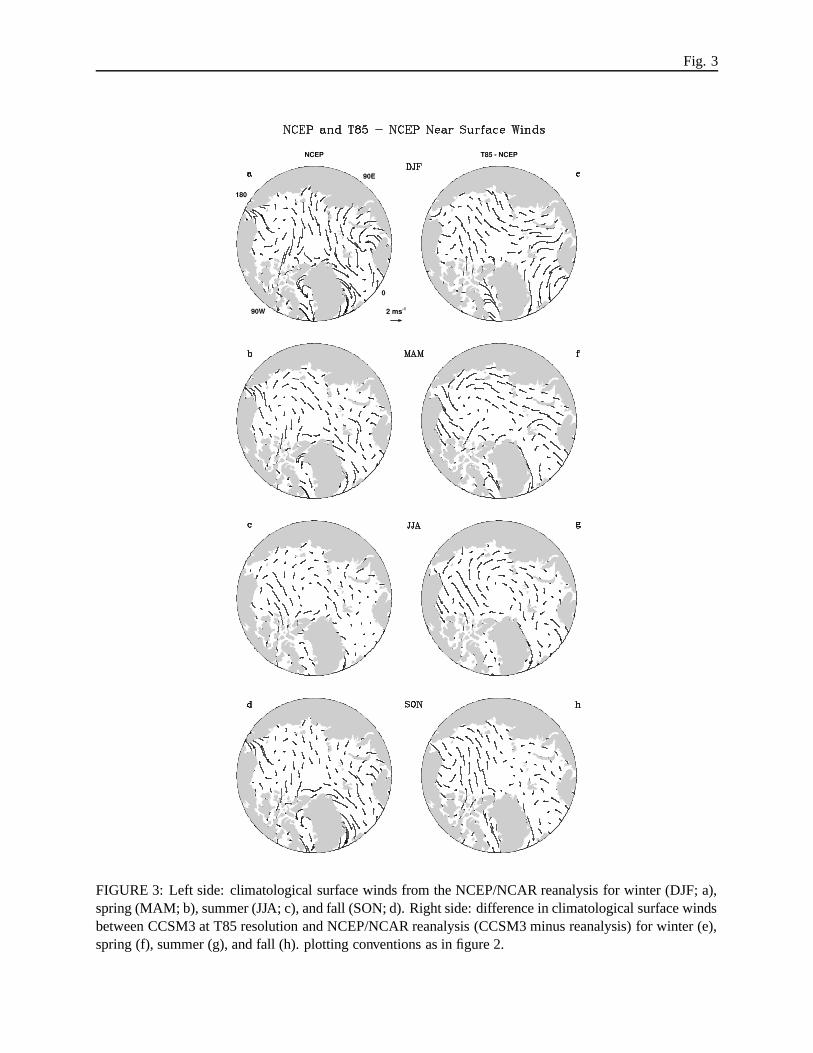
Fig. 3

FIGURE 3: Left side: climatological surface winds from the NCEP/NCAR reanalysis for winter (DJF; a),spring (MAM; b), summer (JJA; c), and fall (SON; d). Right side: difference in climatological surface windsbetween CCSM3 at T85 resolution and NCEP/NCAR reanalysis (CCSM3 minus reanalysis) for winter (e),spring (f), summer (g), and fall (h). plotting conventions as in figure 2.

Fig. 4

NC

EP

0.5

0.5

1

1 11

1.5

2 2

2

2

2.5

33.

54

4

Ann

ual

0.5

1

1

1.5

22

2 2

2

2

2.5

3

33

3.5

4

44

55

Apr

il 0.511

1

1.5

22.

5 33

44

Sep

tem

ber

T42

0.5

0.5

11

1

1

2

2

2 22

2.5

2.53

33

4

0.5

1

1

1.5

1.5

2

22

2.5

2.5

3

3

3 3

3

3.5

3.5

4

4

5 0.5

1

1

1

1

1.5

1.5

1.5

22

2

2.5

T85

0.5

0.5

1

1

1

2

2

2

2

2.5

2.5

3

33

3.5

4

0.5

1

1

1.51.

52

2

2.5

3

33

3.5

3.5

4

4

4.5

5

1

1 1

1.5

1.5

2

2

2

2

2.5

2.5

2.5

3

FIGURE 4: Simulations from an offline sea ice model forced with surface geostrophic winds from theNCEP/NCAR reanalysis (left column) and CCSM3 at T85 (center) and T42 (right) resolution. Annual-mean, April, and September sea ice thickness are shown in the top, middle, and bottom rows, respectively.Contour interval is 0.25m.

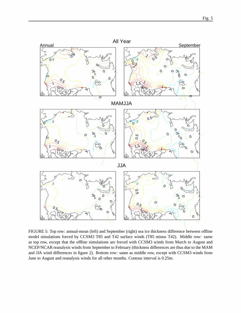
Fig. 5

0

0

0

0

0

0

0

0.5

0.5

1

All YearAnnual

0

0

0

0

00

00

0

0

0.50.5

1

1

1

11.5

2

September

0

0

0

0

0

0

0.51

MAMJJA

0

00

0

0

0

0

0

0.5

0.5

0.5

111.5

2

0

0

0

0

0

0

00

0.5

JJA

0

0

00

00

0

0.5

0.51

FIGURE 5: Top row: annual-mean (left) and September (right) sea ice thickness difference between offlinemodel simulations forced by CCSM3 T85 and T42 surface winds (T85 minus T42). Middle row: sameas top row, except that the offline simulations are forced with CCSM3 winds from March to August andNCEP/NCAR reanalysis winds from September to February (thickness differences are thus due to the MAMand JJA wind differences in figure 2). Bottom row: same as middle row, except with CCSM3 winds fromJune to August and reanalysis winds for all other months. Contour interval is 0.25m.

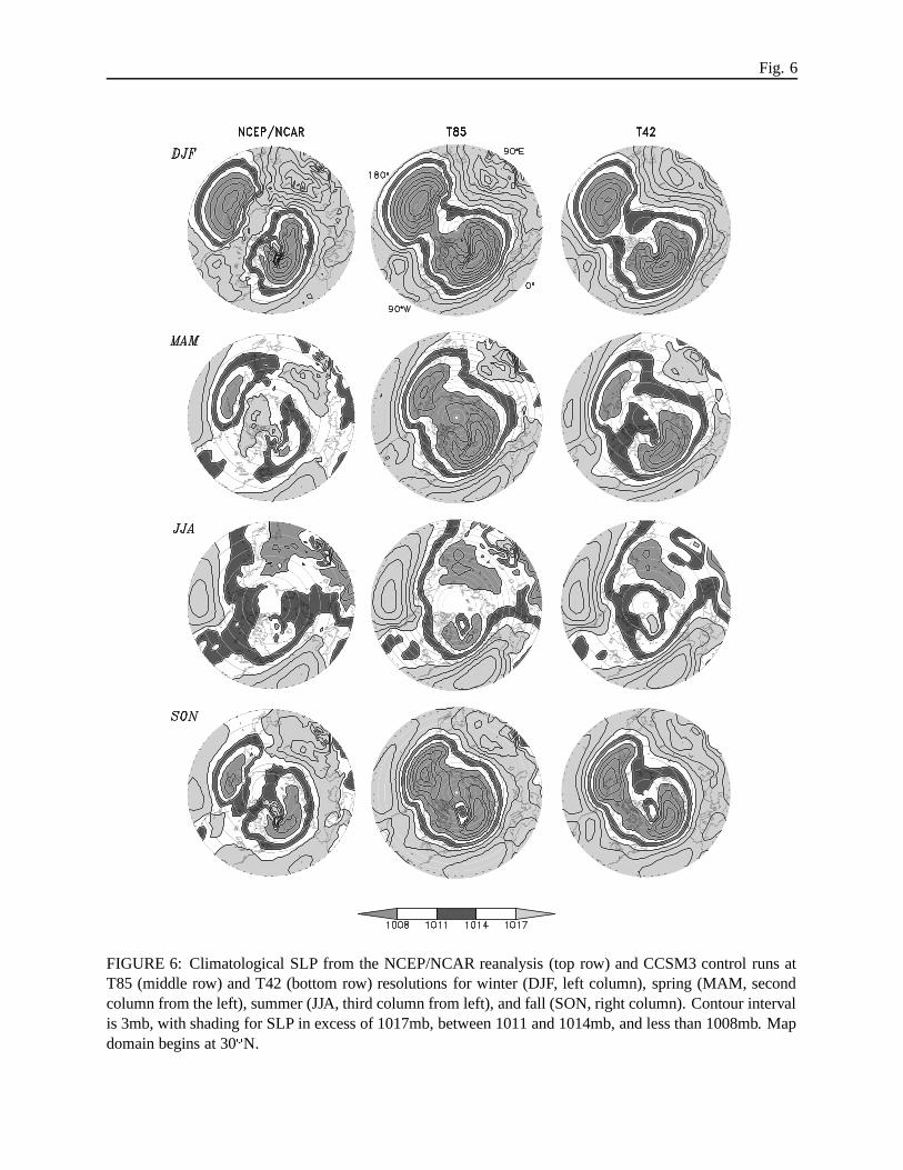
Fig. 6

FIGURE 6: Climatological SLP from the NCEP/NCAR reanalysis (top row) and CCSM3 control runs atT85 (middle row) and T42 (bottom row) resolutions for winter (DJF, left column), spring (MAM, secondcolumn from the left), summer (JJA, third column from left), and fall (SON, right column). Contour intervalis 3mb, with shading for SLP in excess of 1017mb, between 1011 and 1014mb, and less than 1008mb. Mapdomain begins at 30

�N.

Fig. 7

FIGURE 7: DJF Eddy geopotential height at 1000mb (a) and 700mb (b) from the NCEP/NCAR reanalysis.Contour interval in both panels is 25 m, with dark (light) shading for positive (negative) values in excessof 25 m. (c) 1000—100 mb zonal-vertical cross sections of eddy geopotential height and eddy temperatureat 75

�N for NCEP/NCAR reanalysis. Contour interval for eddy height in c is 10m, and eddy temperature

is plotted in 2K contours, with dark (light) shading for positive (negative) values in excess of 2K, and zerocontours suppressed. The whitespace circle in (a) shows the 75

�N latitude circle. Dashed contours denote

negative values in all panels.

Fig. 8

FIGURE 8: DJF Eddy geopotential height at 1000mb for CCSM3 at T85 (a) and T42 (b) resolution. (c) and(d): 1000–100mb zonal-vertical cross sections of eddy geopotential height and eddy temperature at 75

�N

for T85 (c) and T42 (d) integrations. Contours and shading as in the previous figure.

Fig. 9

FIGURE 9: JJA zonally averaged SLP for CCSM3 at T85 and T42 resolution (a), and for the NCEP/NCARand ERA-40 reanalyses (b), and zonally averaged surface zonal wind for the T42 and T85 CCSM3 integra-tions and the NCEP/NCAR reanalyses (c). In all panels, dotted (dashed) curves represent the T85 and T42integrations, and solid lines are used for the NCEP/NCAR reanalysis. In (b) the dashed-dotted line showsthe ERA-40 reanalysis.

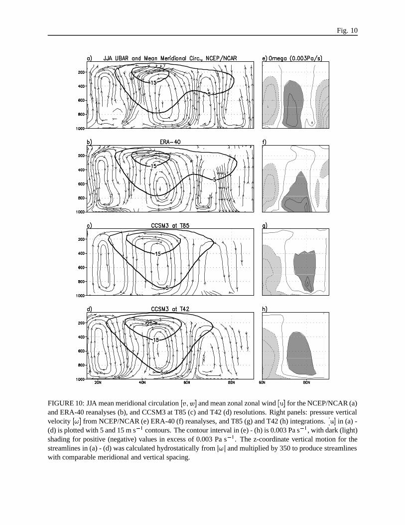
Fig. 10

FIGURE 10: JJA mean meridional circulation ��� 5" �68� and mean zonal zonal wind ������ for the NCEP/NCAR (a)and ERA-40 reanalyses (b), and CCSM3 at T85 (c) and T42 (d) resolutions. Right panels: pressure verticalvelocity �&�%'� from NCEP/NCAR (e) ERA-40 (f) reanalyses, and T85 (g) and T42 (h) integrations. ����5� in (a) -(d) is plotted with 5 and 15 m s ��� contours. The contour interval in (e) - (h) is 0.003 Pa s ��� , with dark (light)shading for positive (negative) values in excess of 0.003 Pa s ��� . The z-coordinate vertical motion for thestreamlines in (a) - (d) was calculated hydrostatically from �$�%'� and multiplied by 350 to produce streamlineswith comparable meridional and vertical spacing.

Fig. 11

FIGURE 11: JJA column-mean meridional flux of zonal momentum from the NCEP/NCAR reanalysis andCCSM3 by sub-monthly transients (a) and the time-mean JJA flow (b), as described in section 6. (c) JJAcolumn-mean sub-monthly transient kinetic energy from NCEP/NCAR reanalysis and CCSM3. (d) 200mbmomentum flux by bandpass filtered transients with timescales of � 2 – 6 days (see section 6 for details).(e) Kinetic energy of transients used in panel (d). (f) 200mb momentum flux by low pass filtered transientswith timescales greater than 10 days. In all panels, solid lines show the reanalysis, dashed lines show theT42 integration, and dotted lines depict the T85 integration. Units are m / s � / .