Atmosphere Analyses Summary of the GLI -...

NASDA Earth Observation Research Center

Summary of the GLI Atmosphere Analyses

GLI Algorithm Integration Team (GAIT)Atmosphere Group

NASDA EORC Contents:1. About GLI atmosphere analyses2. System flow of GLI atmosphere3. GLI algorithm list (Atmosphere)4. GLI standard product list (Atmosphere)5. GLI channel specification6. Summaries of GLI algorithms (Atmosphere)7. References


Abuot GLI atmosphere analyses

Cloud, aerosol, and water vapor parameters

Our inability to adequately model cloud processes is a major obstacle in accurate simulations of global warming

scenarios. Low-level clouds and upper-level clouds play different roles in the climate system. How they change

through the global warming process is, at present, not fully understood. Aerosols are also important for the

global warming issue, as revealed by several recent studies on direct aerosol and indirect cloud-aerosol

interaction effects on the Earth's climate. It is, therefore, important to generate global archives of geophysical

parameters related to cloud, aerosol, and water vapor fields. Using these data sets, we should study the global

distribution, annual variability, and feedback mechanisms of the climate field.

*Water vapor algorithms and products will be appeared in future.


Level-1B

ATSK1,2 / CTSK1

CLFLG_pLevel-2A_OA

OATSKD

ATSK_3p ATSK16

ATSK3_r ATSK3_e

ATSK5

ATSKD

segment data

Daytime

CLTT CLERCLOP CLHT

CLWP

CLOP_pCLFR

foreach cloud type

Nighttime

CLOPCLERCLTT

AROPARAE

Generated by Order - Simple, scene -

Generated by Planning - More details, global -

Sys

tem

Flo

w o

f G

LI A

tmo

sph

ere

Algorithm module

Data


GLI Algorithms (Atmosphere)

# CategoryA: Standard Algorithm (Scene Analysis, approx.1600kmx1600km)B: Standard Algorithm (Global Segment Analysis, 0.25degs lat. lon.)

CategoryPrincipal

InvestigatorProduct Code Name Remarks

ATSKD A NASDA Atmospheric Segment DataGlobal Segment DataGeneration

ATSK1, 2 AStevenAckerman

CLFLG_p Cloud Mask (Scene)

ATSK3_p ATeruyukiNakajiima

CLOP_p Cloud Properties (Scene)

ATSK3_r BTeruyukiNakajima

CLOP, CLER, CLHT, CLTT,CLWP

Cloud Properties (Global,water cloud)

ATSK3_e BTeruyukiNakajima

CLOP, CLER, CLTTCloud Properties (Global, thinice cloud)

ATSK5 BTeruyukiNakajima

AROP, ARAE Aerosol Properties (Global)

ATSK16 B Tamio Takamura CLFR Cloud Fraction


GLI Standard Product List (Atmosphere)

Product Name Global(4days) Global(16days) Global(1 month) Scene UnitCLFLG_p Cloud Flag - - - o -

CLFR

CloudFraction foreach cloudtype

o o o - -

CLOP(_p)Cloud OpticalThickness o o o o (_p) -

CLER

CloudEffectiveParticleRadius

o o o - micron

CLHTCloud TopHeight

o o o - km

CLTTCloud TopTemperature o o o - K

CLWPCloud LiquidWater Path

o o o - g/m^2

AROP

AerosolOpticalThickness at500 nm

o o o - -

ARAEAerosolAngstromExpoment

o o o - -

Data aviilabilityGlobal : Global distribution (0.25degs resolution), generaged by planning4days : 4 days average16days : 16days average1 month : 1 month averageScene : 1 scene product (approx.1600km x 1600km), generated by order

Sample: CLOP by Global (1 month)

Sample:CLOP_p by Scene


CH Wave-length

Band-width

Lmax(H/L gains)

Lstd SNR IFOV Primary Targets

nm nm W/m2/sr/µm W/m2/sr/µm m /rad.1 380 10 683 59 467 DOM (Dissolved Organic Matter) absorption, Land Aerosol2 400 10 162 70 1286 Baseline of DOM3 412 10 130 65 1402 Chlorophyll absorption, DOM absorption, Land Aerosol4 443 10 110/680 54 893 Chlorophyll absorption5 460 10 124/769 54 880 Carotinoid absorption, Snow impurity6 490 10 64 43 1212 Plankton (Carotinoid, Phycobiline)7 520 10 92/569 31 627 Pigment8 545 10 96/596 28 611 Phycobiline absorption, Vegetation9 565 10 39 23 1301 Fluorescence Minimum Absorption

10 625 10 39 17 1370 Phycobiline absorption11 666 10 31 13 1342 Baseline of Fluorescence, Atmospheric Correction12 680 10 33 12 1293 Natural Fluorescence13 678 10 522 12 235 Chlorophyll abs., Aerosol Optical Thickness, Vegetation14 710 10 24 10 1404 Baseline of Fluorescence15 710 10 369 10 300 Sea Ice Monitoring, Vegetation16 749 10 17 7 991 Atmospheric Correction17 763 8 473 6 293 Cloud Geometrical Thickness18 865 20 13 5 1309 Atmospheric Correction19 865 10 339 5 386

1000/1.25

Cloud and Aerosol Optical Thickness, Snow Grain Size20 460 70 691 36 241 Vegetation Classification etc.21 545 50 585 25 141 Vegetation Classification etc.22 660 60 156 14 255 Vegetation Classification etc.23 825 110 287 21 218

250/0.3125

Vegetation Classification etc.24 1050 20 227 8 381 Moisture, Snow Cover, Cloud Optical Thickness25 1135 70 184 8 412 Waver Vapor Amount26 1240 20 208 5.4 303 Moisture, Snow Grain Size27 1380 40 153 1.5 192

1000/1.25

Water Vapor Amount, Upper Cloud Detection28 1640 200 76 5 298 Cloud Effective Radius, Cloud Phase, Snow Grain Size29 2210 220 32 1.3 160

250/0.3125 Cloud Effective Radius

CH Wave-length

Band-width

DynamicRange

TargetTemp.

NEdT(Cold/Hot TV)

IFOV Primary Targets

µm µm K K K m /rad.H: 300 0.07/0.0730 3.715 0.33 345

L: 250 0.71/0.78

Cloud Effective Radius

285 0.02/0.0331 6.7 0.5 307

200 0.27/0.32

Water Vapor Index

300 0.02/0.0332 7.3 0.5 322

200 0.24/0.27

Water Vapor Index

300 0.02/0.0233 7.5 0.5 324

200 0.21/0.24

Water Vapor Index

300 0.03/0.0534 8.6 0.5 350

180 0.47/0.49

Water Vapor Amount, Temperature

300 0.04/0.0535 10.8 1.0 354

180 0.24/0.30

Temperature

300 0.04/0.0636 12.0 1.0 358

180 0.23/0.27

1000/1.25

Temperature

GL

I ch

ann

el s

pec

ific

atio

nVNIR and SWIR channels

MTIR channels


ATSK1,2

Abstract The GLI cloud mask will indicate whether ag i v e n v ie w o f t he e a r t h s u r f a c e i sunobstructed by clouds or optically thickaerosol, and whether that clear scene iscontaminated by a shadow. The cloud maskwill be generated at 1-km resolution. Input tothe cloud mask algorithm is assumed to becalibrated and navigated Level-1B radiancedata. The strategy for this cloud mask algorithm isto start with single pixel (1-km field of view)tests. Many of the single pixel tests rely onradiance (or temperature) thresholds in theinfrared and reflectance thresholds in thesolar. These thresholds vary with surfaceemissivity, with atmospheric moisture andaerosol content, and with GLI viewing scanan gle . The 32bi ts of Cloud f lags w er eobtained from ATSK1,2 together with CTSK1in cryosphere analyses.

Input : Level-1B dataOutput : CLFLG_pP.I. : Steven A. Ackerman (SSEC,University of Wisconsin)A.D. : Richard Frey (SSEC, University of Wisconsin)A.I: Masaru Tairadate (Fujitsu)

Cloud Mask (Scene)

Table CLOUD MASK BIT CONFIGURATION

bitfield

AlgorithmDescription Key

0-1 ATSK1,2 Unobstructed FOV Quality Flag

00 = cloud01 = 66% prob. clear10 = 95% prob. clear11 = 99% prob. clear

2 Processing Path Flags Day / Night Flag 0 = Night / 1 = Day3 Sunglint Flag 0 = Yes / 1 = No4 Snow / Ice Background Flag 0 = Yes/ 1 = No

5-6 Land / Water Flag 00 = Water/ 01 = Coastal10 = Desert / 11 = Land

7 Additional Information Non-cloud obstruction Flag 0 = Yes / 1 = No8 Thin Cirrus Detected (solar) 0 = Yes / 1 = No9 Shadow Found 0 = Yes / 1 = No10 1-km Cloud Flags Result from Group I Tests 0 = Yes / 1 = No11 Result from Group II Tests 0 = Yes / 1 = No12 Result from Group III Tests 0 = Yes / 1 = No13 Result from Group IV Tests 0 = Yes / 1 = No14 Result from Group V Tests 0 = Yes / 1 = No15 reserved for ATSK4161718

19 Dummy Flag 0 = not dummy / 1 = dummy(valid for bit 1-20)

20 Using Channel Flag Used channel 28 and 29 0 = not used / 1 = used(valid for bit 1-20)

21 CTSK1 Snow/Cloud descrimination Execution flag0 = not executed / 1 =executed(valid for bit 21-26)

22-23 Cloud confidence level flag

00 = clear sky01 = high-confidence cloudy confidence = 100%10 = middle-confidence cloudy 50% < confidence < 100%11 = low-confidence cloudy 0% < confidence < 50%

24-26 Surface classification flag

000 = snow over ice001 = sea ice010 = cloud shadow011 = land100 = open water101 = snow over land111 = spare

27-31 Spare

<Acronyms>P.I. : Principal InvestigatorA.D. : Algorithm DeveloperA.I. : Algorithm Integrator


ATSK3_p

Abstract A method for satellite remote sensing of cloud microphysics has beendeveloped to apply to GLI/ADEOS-II multispectral radiance data. Thisalgorithm is an enhanced algorithm of AVHRR/NOAA data analysis (Nakajimaand Nakajima1995; Kawamoto 2000), which has an active thermal collection inabsorption channel. Undesirable radiation components such as ground-reflected solar radiationand thermal radiation are guessed from satellite-received radiances inchannels 13 or 19 (678 or 865 nm), 30 (3.715 µm) and 35 (10.8 µm) of GLIand subtracted from radiances in channels 13 and 30 to derive the reflectedsolar radiation of a cloud layer which includes information about cloudmicrophysical properties. This method can be applied to a broad range ofwater clouds from semi-transparent to thick clouds. The ATSK3_p is designed to analyze every scene of Level-1B data.

Input : Level-1B data, CLFLG_p (from ATSK1,2/CTSK1)Output : CLOP_pPrincipal Investigator : Teruyuki Nakajima (CCSR, University of Tokyo)Algorithm Developer : Takashi Y. Nakajima (EORC, NASDA)Algorithm Integrator : Masaru Tairadate (Fujitsu)

Cloud Properties (Scene)

Sample View:Cloud optical thickness retrieved from MODIS/Terradata (off the coast of California). This result wasobtained using GLI /ADEOS-II analy sis sy stemdeveloped in EORC/NASDA. M OD IS data wereprovided by NASA.


ATSK3_r Cloud Properties (Global)

Input : Segment dataOutput : work_r_w, work_r_iP.I.: Teruyuki Nakajima (Univ. Tokyo)A.D. : Takashi Y. Nakajima (NASDA)A.I. : Masaru Tairadate (Fujitsu)

Sample View:Global distribution of cloud optical thicknessretrieved from MODIS/Terra data. Monthlymean values from September13 to October 12in 2000. These results were obtained usingGLI/ADEOS-II analysis system developed inEORC/NASDA. MODIS data were provided byNASA.

Abstract A method for satellite remote sensing of cloud microphysics has beendeveloped to apply to GLI/ADEOS-II multispectral radiance data. Thisalgorithm is an enhanced algorithm of AVHRR/NOAA data analysis (Nakajimaand Nakajima1995; Kawamoto 2000), which has an active thermal collection inabsorption channel. Undesirable radiation components such as ground-reflected solar radiationand thermal radiation are guessed from satellite-received radiances inchannels 13 or 19 (678 or 865 nm), 30 (3.715 µm) and 35 (10.8 µm) of GLIand subtracted from radiances in channels 13 and 30 to derive the reflectedsolar radiation of a cloud layer which includes information about cloudmicrophysical properties. This method can be applied to a broad range ofwater clouds from semi-transparent to thick clouds. The ATSK3_r is designed to analyze the atmospheric segment data.forglobal scale analyses.



ATSK3_p & ATSK3_r flow chart

I n the ATSK3_p process, radiance of non -absorbing channel (Lch13, or Lch19), ground albedo(Ag), and scan geometries are used to calculatecloud optical thickness (CLOP_p).

On the other hand, the ATSK3_r processneeds non-absorbing channel (Lch13, or Lch19),absorbing channel (Lch30), and thermal channel(Lch35), ground albedo (Ag), and some objectivean al ysis data such as ver t i cal p ro f iles o ftemperature, pressure, and relative humidity, toobtained optical thickness (CLOP), effective radius(CLER), cloud liquid water path (CLWP), cloud toptemperature (CLTT) and cloud top height (CLHT). Pre-process and pos t-process program arerequired to select target pixels from radiancedataset and select suitable results from all outputs.


Input : Segment dataOutput : work_eP.I : Teruyuki Nakajima (CCSR, University of Tokyo)A.D.: Shuichiro Katagiri (EORC, NASDA)A.I. : Shuichiro Katagiri (EORC, NASDA)

ATSK3_e

Abstract Th is al gori t hm w i l l re tr ieve thin c i r rus c loudmicrophysical parameters, effective particle radius,optical thickness and cloud top temperature fromchannels (3.715 µm), 35 (10.8 µm), and 36 (12.0 µm).Figure 1 (next page) illustrates the flow of the algorithm.And Figure 2 illustrates the finding process (ProcessingA in Fig.1) of cloud top temperature and the surfacetemperature (or the cloud top temperature of the cloudlying under the high cloud). Fig.3 shows examples forthe Look-Up Table in the algorithm and the row data intest-run (using AVHRR/NOAA data).

Cloud Properties (Global, thin ice cloud)

Sample View:Global distribution of cirrus cloud optical thick-nessretrieved from MODIS/Terra data. Result of one dayanalysis in December, 2000. This result was obtainedusing GLI/AEOS-II analysis system developed inEORC/NASDA. MODIS data were provided by NASA.



Segment Data(100 data per pixel)

Satellite Data

10.8µm10.8-11.8 µm3.7-10.8 µm

Surface Temperature,Effective Water Vapor

from ancillary data

Effective Radius,Optical Thickness

Temperature of Ground orLow Cloud Initial Condition

Tg [k]Effective Water Vapor

Wef

Table A10.8 µm vs. 3.72-10.8 µm

Table B10.8 µm vs. 10.8-11.8 µm

Fix Ground or Low CloudTemperatureTg = Tg - 0.5

Fix Effective Water Vapor→→→→Wef Wef (new)

No Retrieved

Temperature of Cloud Top InitialCondition Tc[K]

Fix Coud TemperatureTc = Tc - 0.5

ATSK3_e flow chart

Fig.1 The flow chart of the retrieval algorithm.

Processing A: Fitting Tg and Tc

Processing B: Fitting re and ττττ

No Match with Table A

Average Smallest 10 Effective Radii and their Optical Thickness


Fig.2 The concept of the table fittingThe example of processing A in Fig. 1, here,

AVHRR’s ch3=3.7µm,　ch4=10.8µm, ch5=11.8µm Fig.3 Examples for the table in Algorithm and the rawdata in Testrun (AVHRR)

here, AVHRR’s ch3=3.7µm, ch4=10.8µm, ch5=11.8µm


ATSK5

Sample View:Global distribution of aerosol optical thickness retrievedfrom MODIS/Terra data. Monthly mean values fromSeptember 13 to October 12 in 2000. These resultswere obtained using GLI/ADEOS-II analysis systemdeveloped in EORC/ NASDA. MODI S da ta we reprovided by NASA.

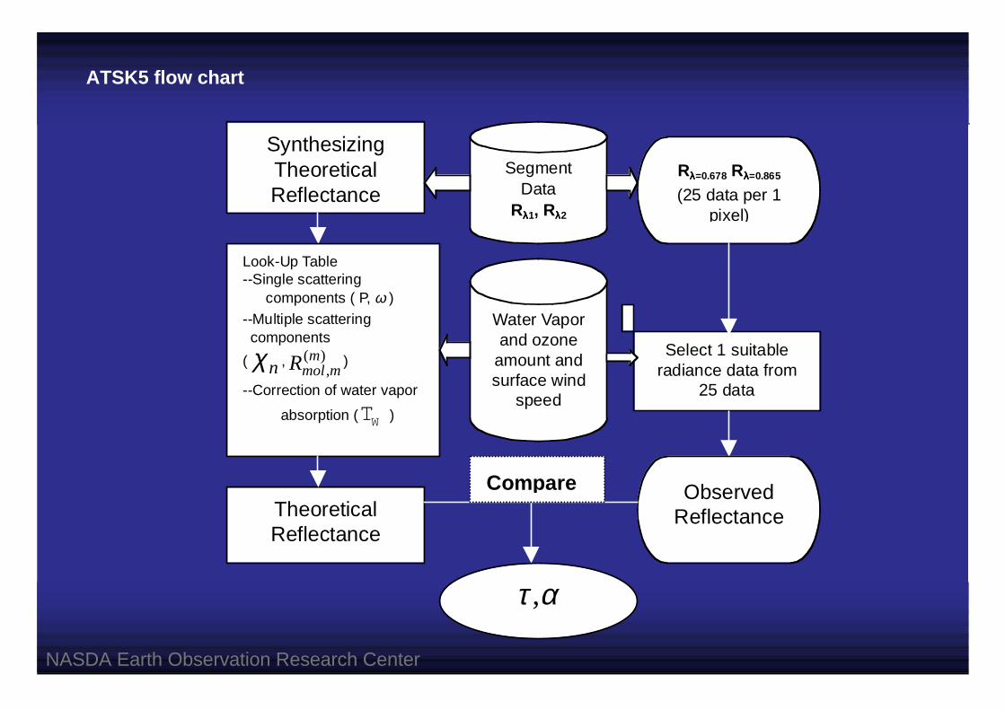
Input : Segment dataOutput : AROP, ARAEP.I. : Teruyuki Nakajima (CCSR, University of Tokyo)A.D. : Akiko Higurashi (NIES, Ministry of Environment)A.I. : Yi Liu (EORC, NASDA)

Aerosol Properties (Global)

Abstract This sa te ll it e remote sensing algori thm retr ievesaerosol opt ical thickness at 500nm and Angstromexponent from two channel radiant data, that is, visible(channel 13, 678nm) and near-IR (channel 19, 865nm)satellite data. Satellite-received radiance is synthesizedwith four Look-Up Tables (LUTs). For retrievals, ancillarydata are needed, which include wind velocity at 10 meterheight, ozone and water vapor amount to correctradiance for surface reflectance, ozone and water vaporabsorption.



Select 1 suitableradiance data from

25 data

SegmentData

Rλλλλ1, Rλλλλ2

Rλλλλ=0.678 Rλλλλ=0.865

(25 data per 1pixel)

Water Vaporand ozone

amount andsurface wind

speed

ObservedReflectance

SynthesizingTheoreticalReflectance

Look-Up Table--Single scattering components ( P, ω )--Multiple scattering components

( χ n , Rmol mm

,( ) )

--Correction of water vapor

absorption ( WT )

TheoreticalReflectance

τ α,

Compare

ATSK5 flow chart


ATSK16

Abstract The algorithm will classify clouds into several types usingoutput data from ATSK3_r and ATSK3_e (The work files. Seethe corresponding pages for details), based on the ISCCPcategories. The characteristics of this algorithm have an indexof cloud shape and an additional classification of cirrus. Thecloud shape can be determined by sum of spatial differencesbetween each pixel in an area of 0.25 degrees square inlatitude and longitude, so a high difference means cumulus-typeand a low one stratus-type. The split window technique willseparate a cirrus cloud from other clouds. The cloud information by the ATSK16 algorithm will be usedfor estimation of surface radiation budget as a research product. The ATSK16 also generates averaged cloud parameters suchas CLOP, CLER and so on from work files of ATSK3_r andATSK3_e.

Input : work_r_w(by ATSK3_r), work_r_i(by ATSK3_r), work_e(by ATSK3_e)Output : CLFR_1-19,

CLOP_w_r, CLER_w_r, CLTT_w_r, CLHT_w_r, CLWP_w_r, CLOP_i_r,CLOP_i_e, CLER_i_e, CLTT_i_e

Principal Investigator : Tamio Takamura (CEReS, Chiba University)Algorithm Developer : Itaru Okada (CEReS, Chiba University)Algorithm Integrator : Yi Liu (EORC, NASDA)

Cloud Fraction

Rossow et al. 1996, ISCCP Documentation of New Cloud Dataset


Ice cloud

CLTP classification

Average CLOP_i_rCLFR_18

Count pixel number:CLFR_10

Index of imhomogeneityof CLTT: CLFR_19

440<CLTP=<680Average CLTT:

CLFR_13Average CLOP:

CLFR_16

CLTP=<440Average CLTT :


CLFR_15

680<CLTPAverage CLTT:


CLFR_17

CLOPclassification

CLOPclassification

CLOPclassification

3.6>CLOPcount pixel number:

CLFR_1

23>CLOP>=3.6

count pixel number:CLFR_2

CLOP>=23count pixel number:

CLFR_3


CLFR_4

23>CLOP>=3.6



CLFR_6


CLFR_7

23>CLOP>=3.6



CLFR_9

ATSK16 flow chart

Yes

No

CLTP: Cloud Top Pressure

Sum of CLFR_1 to CLFR_10

CLFR_11


ReferencesATSK1,2Ackerman, S. A., W. L. Smith and H. E. Revercomb, 1990: The 27-28 October 1986 FIRE IFO cirrus case study: Spectral

properties of cirrus clouds in the 8-12 micron window, Mon. Wea. Rev., 118, 2377-2388.Ackerman, S. A., 1997 : Discriminating clear-sky from cloud with GLI. Development status report to NASDA.Ackerman, S. A., K. I. Strabala, W. P. Menzel, R. A. Frey, C. C. Moeller and L. E. Gumley Discriminating Clear-sky from

Clouds with MODIS, 1998: J. Geo. Res., 103 , D24, p. 32,141ATSK3_p, ATSK3_rNakajima, T. and M. D. King, 1990: Determination of the optical thickness and effective radius of clouds from reflected solar

radiation measurements. Part I: Theory. J. Atmos. Sci., 47, 1878-1893.Nakajima T. Y. and T. Nakajima, 1995: Wide-area determination of cloud microphysical properties from NOAA AVHRR

measurement for FIRE and ASTEX regions, J. Atmos. Sci., 52, 4043-4059.Kawamoto, K., T. Nakajima, and T. Y. Nakajima, 2000: A global determination of cloud microphysics with AVHRR remote

sensing, J. Climate, 14, 2054-2068.ATSK3_eKatagiri, S., 2001: , thesis for doctor degree., University of

Tokyo.ATSK5Nakajima, T., and A. Higurashi, 1998: A use of two-channel radiances for an aerosol characterization from space. Geophys.

Res. Lett., 25(20), 3815-3818.Higurashi, A., and T. Nakajima, 1999: Development of a two Channel aerosol retrieval algorithm on global scale using

NOAA/AVHRR. J. Atmos. Sci., 56, 924-941.Higurashi, A., and T. Nakajima, 2000: A study of global aerosol optical climatology with two channel AVHRR remote sensing.

J. Climate, 13, 2011-2027.ATSK16Rossow, W.B., A. W. Walker, D. E. Beuschet. M. D. Roiter, 1996: International Satellite Cloud Climatology Project

documentation of new cloud dataset. pp39.

Atmosphere Analyses Summary of the GLI -...

Documents

Transcript of Atmosphere Analyses Summary of the GLI -...