Atlantic Meridional Transect AMT-11 Cruise Report

Grimsby (UK) to Montevideo (Uruguay) 12th September to 11th October 2000

AMT11 Cruise Report

Contents

Abstract..................................................................................................................................................... 1 AMT Aims................................................................................................................................................. 1 Acknowledgements................................................................................................................................... 2 Cruise participants................................................................................................................................... 3 AMT-11: Cruise Narrative:..................................................................................................................... 5 Daily Science log....................................................................................................................................... 8 Individual Research Reports................................................................................................................. 21

Mesozooplankton respiration, excretion, and feeding. ............................................................................... 21 Optics.......................................................................................................................................................... 23 Fast Repetition Rate Fluorometry............................................................................................................... 25 Seawater Filtrations .................................................................................................................................... 29 Nitrogen uptake and regeneration............................................................................................................... 30 Bacterial production and abundance........................................................................................................... 30 Phytoplankton-mediated carbon and oxygen flows.................................................................................... 32 Macro-nutrient depth profiles - CDOM depth profiles............................................................................... 35 AutoFlux Trials .......................................................................................................................................... 37 Marine Geophysics ..................................................................................................................................... 56

Appendix 1: Noon Positions AMT-11, Sept/Oct 2000 ......................................................................... 58 Appendix 2: AMT-11, Salinity Bottles, Analysed on the AUTOSAL, 8/10/00.................................. 59 Appendix 3: XBT deployment log......................................................................................................... 60 Appendix 4. Underway night watch, sampling and observation ....................................................... 62

Prepared and edited by: Malcolm Woodward

Principal Scientist: AMT-11.

Plymouth Marine Laboratory Prospect Place

Plymouth Devon

PL1 3DH England

m.woodward@pml.ac.uk

01752 633459 (office): 01752 633100 (switchboard)

AMT11 Cruise Report

1

Abstract This report describes the scientific activities of the eleventh Atlantic Meridional Transect cruise (AMT-11) on board the British Antarctic Survey research vessel the RRS James Clark Ross.

The cruise sailed from Grimsby in the United Kingdom on 12th September 2000, and ended in Montevideo, Uruguay on October 11th.

The long-term objectives of the AMT programme are stated as follows:

• To better understand the links between biogeochemical processes, biogenic gas exchange, air-sea interactions and the effects on and the responses of oceanic ecosystems to climate change.

• To investigate the functional roles of biological particles, and the processes that influence ocean colour in ecosystem dynamics.

• To develop algorithms and the validation of remotely sensed observations of ocean colour. As previously the cruise was centred close to 20 degrees West for the southern transect in the northern hemisphere, the track then deviated to the east to carry out the BAS swath bathymetry research survey, which was essentially a cruise within the AMT. Following this work in the Romanche Fracture Zone, part of the Mid-Atlantic ridge system, the cruise transect headed south-westerly past Ascension Island across the south Atlantic gyre, and on to Montevideo, Uruguay.

The scientific team were a truly international group who all contributed to produce an exceptional cruise from both the scientific and social aspects.

This cruise is sadly the last in the time series of cruises started in 1995 and supported almost entirely through Plymouth Marine Laboratory. This is a great loss of a resource to the UK and international scientific community with these cruises offering an almost unique opportunity for regular long transect scientific research. It is hoped that the UK community will in some way in the future find funding to re-instate the research programme.

AMT Aims

The long-term aims of the AMT programme are: 1. To understand the links between biogeochemical processes, biogenic gas exchange, air-sea

interactions and the effects on, and the responses of the oceanic ecosystems to climate change. 2. To investigate the functional roles of biological particles and processes of ecosystem dynamics which

influence ocean colour, and as such the programme aims towards the development of algorithms and the validation and interpretation of remotely sensed satellite observations of ocean colour.

3. To develop coupled physical-biological models of production and ecosystem dynamics, to improve our knowledge of processes, ecosystem dynamics, food-webs and fisheries, and to characterise biogeochemical oceanic provinces.

AMT11 Cruise Report

2

Acknowledgements

AMT-11 is the eleventh cruise in a series of transects of the Atlantic Ocean using the RRS James Clark Ross (JCR), one of the British Antarctic Surveys’ Research ships.

The series of cruises have used this invaluable opportunity to carry out ‘added value’ science on top of the normal cruise transect legs of the JCR, between the UK and the south Atlantic. The ship goes south in September normally, with the passage leg terminating in The Falklands at Port Stanley, with a regular port-call in Montevideo for supplies. The ship then returns back to the UK after the summer fieldwork season in the Antarctic in May/June of the following year. On AMT-11, for financial reasons, we terminated the cruise in Montevideo.

The AMT science team are most grateful to Prof. Chris Rapley and all his teams in Cambridge, in logistics, personnel, planning, etc. etc. Without whose help and support this cruise and the AMT programme would not be possible.

Also thanks to all our international colleagues on the cruise for the financial support from their home Institutions and Universities.

And finally, the Principle Scientist and the scientific party acknowledge the invaluable assistance of the Officers and crew of the RRS James Clark Ross, led by Captain Jerry Burgan. Their professional skills have contributed hugely to the success of the scientific research of the AMT-11 cruise and the programme as a whole.

AMT11 Cruise Report

3

Cruise participants

This AMT was different to previous cruises in that it coupled a number of projects under the AMT banner. As well as the core scientists for the AMT there were two researchers from SOC carrying out meteorological investigations as part of the ‘Autoflux’ project, and also the newly fitted Swath Bathymetry system on board the JCR was being trialled on the long transect south and also to carry out a specific study of the eastern end of the Romanche fracture zone, just south of the equator.

These three disparate groups worked extremely well together, neither particularly interrupting each others science, and in fact the diversion of the ship to carry out the Swath studies actually gave an excellent scientific opportunity to the core biogeochemists to carry out a number of investigations in the equatorial upwelling area which is greatly under-researched.

Scientific personnel

AMT Group Institute Role Malcolm Woodward PML Principal Scientist AMT, nanonutrients Emilio Fernandez UIV Chlorophyll, primary production Pablo Serrett UIV Oxygen production and Respiration. Ramiro Varela UIV P-I curves, and absorption characteristics. Vassilis Kitidis PML, UIN Nutrients and DOM breakdown. Begona Castro IEO S Bacterial production and abundance. Marta Varela IEO Nitrogen uptake. Claudia Omachi PML Fast Repetition Rate Fluorometry, (FRRF) Dave Suggett PML/SOC Chlorophyll, CHN sampling, Fluorometry Sandy Thomala SOC Chlorophyll, CHN sampling. Alejandro Isla UIO Zooplankton respiration, ammonia production Marcos Lopes UIO Zooplankton biomass, and grazing.

Autoflux group

Margaret Yelland SOC Surface fluxes system Robin Pascal SOC Surface fluxes system

Swath bathymetry group

Alex Cunningham BAS Swath bathymetry Neil Mitchell OX/CU Swath bathymetry

BAS scientific support

Andy Barker BAS IT Support Vsevolod Afanasyev BAS ET Support

Supernumerary Don BONNER Falkland Islands

Key BAS: British Antarctic Survey, High Cross, Madingley Road, Cambridge, CB3 0ET, UK OX: Oxford University, Wellington Square, Oxford, OX1 2JD, UK CU: Cardiff University, Cardiff, Wales, CF10 3XQ, UK PML: Plymouth Marine Laboratory, Prospect Place, Plymouth, PL1 3DH, UK SOC: Southampton Oceanography Centre, European Way, Empress Dock, Southampton, SO14 3ZH, UK IEO: Instituto Espanol de Oceanografia, Centro Costero de la Coruna, Muelle de Animas s/n, A Coruna, E-

15001, Spain UIN: University of Newcastle, Newcastle, NE1 7RU, UK UIO: University of Oviedo, Oviedo, Spain UIV: University of Vigo, Campus Lagoas-Marcosende, 36200 Vigo, Spain

AMT11 Cruise Report

4

Ship’s personnel Name: Rank / Rating: Jerry Burgan Master Graham Chapman Chief Officer Justin McCarthy Second Officer Neil Macleod Third Officer Steve Mee Radio Officer Duncan Anderson Chief Engineer Colin Smith Second Engineer Robert Macaskill Third Engineer Gerry Armour Fourth Engineer Doug Trevett Deck Engineer Anthony Rowe Electrician Hamish Gibson Catering Officer Pippa Bradbury Doctor Russell Brookes Deck Cadet Dean Burnett Engineer Cadet Colin Lang Bosun David Peck Bosun’s Mate Martin Bowen Seaman Kelvin Chappell Seaman George Dale Seaman Keith Dickson Seaman Luke Trussler Seaman Erwin Allen Motorman Richard Parsley Motorman Danny Mcmanamy Chief Cook Tracey Macaskill Second Cook Lee Jones Second Steward Simon Hadgraft Steward Graham Raworth Steward Michael Weirs Steward

AMT11 Cruise Report

5

AMT-11: Cruise Narrative:

The AMT-11 departed from Grimsby on Tuesday 12th September, leaving the lock gates at 0510, and sailed into the North Sea heading for Portsmouth for a port call to take on board aviation fuel.

During the first morning there was carried out a general test of the CTD equipment to ensure all sensors were responding and operational. This was only to a depth of 10 metres. Also the Sound Velocity Profiler (SVP) was tested to ensure all was operational also.

The AMT team had commenced mobilisation in Grimsby (UK) on the Sunday 10th, after arriving the day before. All was smoothly achieved with the help of the crew, in assisting the equipment siting and generally helping the scientists.

During the short passage leg to Portsmouth the various pieces of scientific lab equipment were checked out and there was noticed that due to a valve being left open that we had lost a large amount of the liquid nitrogen stored, so provision was made to replenish stocks at the dockyard, and this was successful. Also, it was found that the Beckman liquid scintillation counter was non functional. As this is imperative to count the radiological experimental samples, I investigated the possibilities of having a repair carried out in Portsmouth. This again was successful, although it was not particularly acceptable to have this instrument non-functional even before sailing. However, the repair was agreed to and completed. The machine ran well for 3 weeks of the cruise, but then had a week of intermittent functioning, but having watched the engineer we were able to carry out ‘running’ repairs. The machine has since recovered its functionality some what but still is prone to jamming. The machine was repaired with a ‘used’ part in order to get it working and a future full repair and service or purchase of a new machine needs to be investigated. However, we did achieve all the counting and analyses of the samples by the end of the cruise.

We sailed from Portsmouth on the evening of the 13th and headed west into the Channel.

One of the main activities that have underpinned all the AMT cruises is the regular sampling of the surface non-toxic seawater. The first sample was taken on the morning of the 14th and then continued at regular 4 hourly intervals, or with greater frequency at scientifically interesting areas, until the end of the cruise. These samples are taken for chlorophyll fluorescence, samples for later HPLC analyses at Plymouth, and for particulate carbon and nitrogen analyses.

Then at 1045 on the 14th we carried out the first of what were 46 CTD stations. The Seabird 911 plus CTD system with a sample bottle rosette of 12x 10 litre bottles was equipped also with the PAR light sensors and with transmission and fluorescence sensors. The system was kept supported by Sevvy and Andy the BAS technical support team. The functionality of the system was 100% with every CTD carried out without a lost bottle or malfunction. An excellent support provided from the two technicians to the cruise and something which is an absolutely vital element to the AMT, and indeed any biogeochemical type cruise, in having a reliable CTD system.

Following this first shallow CTD in the western end of the English Channel, by the next day we had crossed out from the channel to the western approaches, and then out over the shelf break to water depths in excess of 2000 metres. The CTD’s were then standardised to a maximum depth of 250m, with the bottles being fired at targeted biological structures in the water column. The depth was chosen as a compromise between time on station, which is limited, but also to give a sufficient coverage of the water column to ensure that we always went below the mixed layer depth (normally a maximum of 180m in the south Atlantic gyre) and so allowing us to always study the important euphotic zone where the light influences the biological processes. By the cruise end we carried 46 successful CTD stations.

Because of the biological sampling requirements the programme for the daily CTD casts we carried out 2 CTD stations a day. There was first a pre-dawn cast normally timed around 0430, and this was to sample for the production studies, both primary production and for respiration and oxygen production experiments. Concurrently with the CTD were two triple-net casts to 200m with various net sizes attached so as to size fractionate the zooplankton size classes. The zooplankton samples from these net hauls were then used to study biomass, the taxonomic composition and the gut contents of the copepods. Feeding experiments were also carried out by incubating the samples and sub samples were also taken for respiration and excretion.

AMT11 Cruise Report

6

The CTD standard sampling and analysis was, apart from the water for the productivity samplings, for nutrient analysis. This was to study the distributions of nitrate, nitrite, silicate, phosphate and ammonia using conventional colorimetric techniques and also using new novel high sensitivity methods. Samples were also taken to study the distributions of chromophoric dissolved organic matter (CDOM) which is of great importance to the studies of ocean optics and hence to remote sensing by satellites.

The standard filtration samples were also taken for chlorophyll and particulate carbon and nitrogen, and investigations were also made with samples to study bacterial production and abundance.

The samples taken for the production studies were then incubated in the on-deck incubators for up to 24 hours using the ships non-toxic water supply as cooling. Various light fields were simulated using filters to mimic the light intensities experienced by the samples at the depth of water that they were taken from.

The second daily CTD was timed at around 1100, in order to give maximum sunlight irradiance. The standard sampling was carried out for the CTD, except this time the samples were more targeted at studies involving light and its effects on the biota. Standard samples were again taken for filtering and for the nutrients, but with this CTD samplings were carried out to study the photosynthesis/irradiance curves (P/I), which show the relationship between the light irradiance and the rate of carbon incorporated by photosynthetic processes. Samples were also taken for experiments to study the nitrogen uptake and regeneration of the phytoplankton with reference specifically to nitrate, ammonia and urea.

Whilst the CTD operations were taking place there were again net samples taken from the forward davit, one down to 100m for subsamples to later evaluate biomass by image analysis and to determine particulate carbon and nitrogen. A second net sampling for surface qualitative taxonomic phytoplankton samples was then obtained.

A third over the side operation was carried out at this late morning station with the deployment of the optics rig, with attached fast repetition rate fluorometer (FRRF). The optics rig consisted of the fluorometer, a CTD, and a pair of 7-channel irradiance and radiance sensors. The rig was lowered to 150m or 200m in the initial deployment and then to 60m at a second. On a couple of occasions when the sunlight was good with little cloud cover an extra optics cast was carried out during the afternoon.

This then concluded the overside operations for the day, but the underway sampling continued as did the regular deployment of the expendable bathythermographs (XBT), which were deployed to 1830m or 760m at different times of the day.

The station time was of course closely regulated as there was only a finite time for station work, which initially averaged to about 1 hour 45 minutes per day and this was closely regulated. The one problem that there was with this timing was the uncertainty of the actual amount of time allocated to the AMT and to the Swath study. In the ships programme there were 4 days added to passage for the AMT and 2 days for the Swath work. However, it then became apparent that the Swath required 2 days just for the scientific survey and that there was an extra almost 2 days to passage required for the deviation for the ‘normal’ track. This though did not materialise as a problem as the AMT in fact worked a more direct track to that initially considered and so one day was saved there. Then by judicious other means the almost extra day was saved in order that the ship was on time docking into Montevideo. Again, good discussions and communications between all concerned solved the problem before it really became one.

The swath bathymetry studies were ongoing for the cruise where possible as was the ‘autoflux’ studies, which were the continuous logging of the sea temperatures and the heat fluxes generated.

The cruise track took us south and avoided the 200 mile limits (EEZ) of the various Atlantic islands and coastal states. This track was plotted and allowed a maximum of science for a minimum deviation from the ‘standard’ passage. There were no diplomatic clearances for this cruise obtained due to the late decision taken to actually go ahead with the cruise itself. However, this did not seriously impact on the science due to the course taken. The only place where it was impossible to work was a period of about 36 hours between the Cape Verde Islands and Senegal where the overside science was stopped. Just north of the equator and south of these EEZ’s the ‘normal’ AMT track would turn to the south-west to head for south America, but with the requirements of the Swath work we deviated south east to occupy a station at approximately 1°S and 13°W. This was for a detailed survey of the eastern end of the Romanche fracture zone system, a part of the mid-Atlantic Ridge. This proved to be very successful, and indeed was a science of opportunity for the biogeochemists of the core AMT team as we were able to continue sampling an area where the equatorial upwelling was very strong. This is an area, mainly because of its

AMT11 Cruise Report

7

remoteness, that is very understudied, and some excellent new investigations were carried out. The fact that the CTD casts and biogeochemistry could be continued shows an evolution in the possible way forward and future for the AMT programme. It is hoped that there will be future collaborations with the Swath science and the future AMT cruises, giving an extra dimension to the scientific findings.

After leaving the Swath study area there was then almost a straight track to Montevideo, except for a small deviation to carry out an opportunistic survey of an undersea volcano site close to Ascension Island. The last 11 days were across the oligotrophic, or ‘marine desert’ of the south Atlantic Gyre, again giving a huge contrast to the productive area of the equatorial upwelling south of the equator.

The final CTD was on Monday 9th October, and the underway ceased also at 1400 the same day.

A very successful cruise, aided in great part by a good sound working relationship and excellent communications between the science team and the captain and officers. Any problems there were, were dealt with simply and quickly.

AMT11 Cruise Report

8

Daily Science log

12/9/00 Sailed from Grimsby at 0505, Tuesday 12th September. On station at 1030, test Station, 53006’1N 01019.5’E Depth 17m, heading 255. 1044: CTD in the water to 10m, Optics deployed to 15m, then recovered at 1101. 1104: SVP (Sound Velocity profiler) deployed 1116: SVP recovered 1125: off station Followed by test XBT deployment. Science get together of all the science people with AMT, SOC and Swath people + BAS support guys.

13/9/00 0312: Commenced magnetic calibration turns for the SOC Autoflux lab equipment, consisting of 2 360’ turns to starboard, then resume course for Pompey. 0750: Docked at Portsmouth. Commenced the aviation fuel replenishment. Some of the Team ashore. Visit from Patrick Holligan and Mike Lucas in am. 1130: Delivery of liquid nitrogen from Cryospeed, very efficient and cheap ! 1400; John Butler the Beckman engineer arrived to repair the Liquid Scintillation counter. Good guy, gave an air of confidence. Fixed the machine by 1800 and serviced it. All calibrated and up to spec, excellent! Emilio is very happy, and BAS are picking up the tab. Main problem was that it was not serviced this year as it is on a 2 year cycle of servicing. A short sighted idea, they (David Blake) have since commented as that AMT is only user and with the uncertainty of its future basically why bother to spend any money on it if they (BAS) have to. Oh dear ! Sailed Portsmouth at about 1900, nice evening, good sunset, team in good spirits, morale high and prospect of good science is high. Science meeting of the AMT core scientists to discuss the first CTD and the underway sampling protocols. Water volumes etc discussed and detailed below: SCIENTIST 0430 CTD 1100 CTD WHAT FOR VOLUME Marta NO YES - 6 litres (3depths) Alejandro, Marcos YES YES Zooplankton net

samples + Chloro a at mid am CTD

30 litres from the chlorophyll max

Begonia YES NO Bacterial Production 100 ml, 5 depths Malc and Vas YES YES Nutrients, micro and

nano 500mls

Sandy/Claudia/Dave NO YES HPLC 4 litres all depths S/C/D NO YES Chlorophyll a 250mls, all depths S/C/D NO YES Coccolithophores 200mls all depths S/C/D YES YES CHN 2 litres all depths S/C/D NO YES FRRF/PI 350mls S/C/D YES NO FRRF 250mls S/C/D NO YES Absorption 250mls Pablo YES NO Oxygen product and

Respiration 4 litres, 5 depths

Ramiro NO YES PI curves 1.5 litres, 3 depths Ramiro NO YES Absorption 3 litres, 3 depths Emilio YES NO Primary product. 1.5 litres, 5 depths Emilio NO YES Size fractionated PP 250mls, all depths

AMT11 Cruise Report

9

Also: Dave Suggett to carry out a surface net haul during the mid am CTD station at the same time as the optics rig deployment and CTD. Emilio will add a net deployment to 100 metres prior to this. 250 metres will be the bottom bottle. On station, ship with sun on starboard, and the request of Autoflux that the ships head is to windward or as near as possible during the CTD.

14/9/00 1053: Commenced first station (AMT 11/01), approx directly south of Plymouth, CTD deployed to 60m, Optics deployed to 80m. Plus nets. 1119: Finish and proceed. 1132 XBT launch 1702 XBT launch 2250 XBT launch

15/9/00 0417: CTD deployed to 250m, nets deployed forward, two deployments to 200m 0447: CTD recovered 0456 Nets recovered 0500: Depart station and on course 0530: XBT launch, failed (a bad box of probes, change box) 0552: XBT launch (OK, successful). 0946: On station: AMT 11/03 0952: Optics deployed (150m), CTD deployed (250m), and surface nets forward deployed 1006: Sound velocity Profiler (SVP) deployed from the port gantry, to 500m. (Involved with the Swath work). 1009: Second Optics cast (100m). Nets recovered, CTD onboard. 1018: SVP recovered 1022: Proceeding 1122: XBT launch 1637: XBT launch 2303 XBT launch

16/9/00 0420: Commence slowing for station 0434: CTD deployed (AMT 11/04) (250m) 0438: Forward nets deployed, 0451: CTD on deck 0453: Nets recovered 0500: On course and departed. 1049: On station, CTD deployed (AMT 11/05) (250m). Nets to 100m deployed. Optics deployed to 150m. 1101: Nets recovered, and surface nets redeployed. 1111: Optics rig redeployed to 60m 1113: CTD on deck 1114: optics recovered and nets. 1128: XBT deployed, and underway on track and speed. 1212: XBT launched 1912: XBT launched 2342: XBT launched

AMT11 Cruise Report

10

17/9/00 0425: On station, CTD (AMT 11-06) (250m) 0434: Nets deployed to 200m. 0447: Nets recovered and redeployed to 200m 0452: CTD recovered 0506: Nets recovered 0512: On course and speed 0533: XBT launch 1044: On station, CTD (AMT 11-07) (250m) 1047: Nets to 100m and Optics deployed to 150m 1055: Nets recovered and redeployed to surface. Optics recovered 1109: CTD on deck and nets recovered 1120: XBT deployed 1125: On track and proceeding 2346: XBT launch

18/9/00 0443: On station, CTD (AMT 11-08) (250m) 0448: Forward nets deployed to 200m 0451: CTD deployed to 250m 0502: nets recovered and redeployed to 200m 0511: CTD on deck 0521: Nets recovered 0527: On course and proceeding 0643: XBT launched 1044: On station CTD (AMT 11-09) 1046 Nets to 100m deployed and Optics to 150m, and CTD deployed 1053 Nets recovered, and redeployed for surface netting 1101: Optics recovered and then redeployed to 60m 1106: nets recover, CTD on deck and optics recovered 1119: XBT launch at 6 knots, deep XBT (1830m, T5) 1123: Underway and departed. 1754: XBT launched, T7 2340: XBT launched, T7

19/9/00 0444: On station, CTD (AMT 11-10) (250) 0448: Forward nets deployed (200m) 0449: CTD deployed. 0502: Nets recovered 0505:Nets redeployed to 200m 0510: CTD on deck 0520: Nets recovered. 0526: On course and speed. 0601; XBT launch 1045: On station 1046: Nets deployed forward to 100m 1048: CTD deployed to 250m (AMT 11-11) 1050: Optics deployed to 150m 1053: Nets recovered

AMT11 Cruise Report

11

1056: Nets launched to surface water 1105: Redeploy optics to 60m 1106: Nets recovered and CTD on deck 1110: Optics recovered 1122: XBT launched, T5 to 1830m 1723: XBT launched, T7 2346: XBT launched, T7

20/9/00 0444: JCR on station. 0445: Nets deployed to 200m 0447: CTD deployed to 250m (AMT 11-12) 0500: Nets recovered 0509: CTD recovered 0519: On course and speed 0609: XBT launched 1045: On station 1046: Nets deployed to 100m. Optics deployed to 150m 1048: CTD deployed to 250m (AMT 11-13) 1053: Nets recovered 1056: Nets redeployed to the surface 1102: Optics recovered and redeployed to 60m 1105: Nets recovered 1107: CTD on deck 1109: Optics recovered 1121: XBT launch, T5 to 1830m 1300: AMT team science meeting to confirm plans for the following couple days, check sampling strategy etc with everyone. 1745: XBT launch, T7 2343: XBT launch, T7

21/9/00 0444: On station 0446: Nets deployed forward, to 200m 0448 CTD deployed (AMT 11-14) to 250m 0501: Nets recovered 0503: Nets redeployed to 200m 0509: CTD on deck 0519: Nets recovered forward 0606: XBT launch, T5. 1043: On station, 1046: Nets to 100m deployed 1047: Optics rig deployed to 150m 1049: CTD deployed to 250m (AMT 11-15) 1053: Nets on-board, Redeploy to surface water 1102: Optics recovered and redeployed to 60m 1107: Optics and nets recovered. 1109: CTD recovered. 1121: Three XBT launches with T5’s. Terminations and errors for first two, ship slowed to 6 knots to deploy them.

AMT11 Cruise Report

12

1612: Slow to 6 knots and launch T5 XBT, still problems, needed two attempts 1947: Slow to 6 knots for deep T5 XBT 2337: Slow to 6 knots for deep T5 XBT 2359: Cease science overside operations during passage through Cape Verde and Senegal EEZ’s.

22/9/00 Container cleaning/rubbing down and painting, followed by fire drill and practice of fire extinguishers and hoses on deck. Data work-up and general lab preparation.

23/9/00 1045: On station, 1046: Nets to 100m deployed 1047: Optics to 150m deployed 1049: CTD deployed to 250m (AMT11-17) 1053: Nets recovered 1056: Surface nets deployed 1102: Optics recovered 1103: Optics redeployed to 60m 1106: Nets recovered 1108: CTD on deck and Optics recovered 1123: Deep XBT, to 1830m, T5 probe. 1717: XBT (T7) deployed 2347: XBT deployed, T7

24/9/00 0445: On station 0446: Forward nets deployed to 200m 0449: CTD deployed to 250m, (AMT11-18) 0502: Nets recovered 0503: Nets redeployed to 200m 0511: CTD on deck, 0519:Nets recovered 0811: XBT launch, T5 to 760m 1046: On station 1048: Optics deployed to 150m 1050: CTD deployed to 250m, (AMT 11-19 1054: Nets deployed forward to 100m 1101: Nets recovered 1103: Nets redeployed forward to surface water 1104: Optics rig redeployed 1107: CTD on deck 1108: Nets recovered 1110: Optics recovered 1121: XBT launch to 1830 metres, T5. 1500: On station 18a 1501: Deploy CTD to 15m (AMT11-18a). Four drops to 15m for calibrations of temperature sensors. 1502: Optics deployed to 150m 1517: Optics recovered 1518: CTD recovered 1734: XBT launch, T7 to 760m. 2345: XBT launch, T7 to 760m

AMT11 Cruise Report

13

25/9/00 0445: On station 0447: Forward nets deployed to 200m 0449: CTD deployed to 250m (AMT11-19) 0503: Nets recovered 0505: Nets redeployed to 200m 0511: CTD recovered on deck. 0522: Nets recovered forward 0526: On course 1045: On station 1046: Nets to 100m deployed forward 1047: Optics deployed to 150m 1050: CTD deployed to 250m (AMT 11-20) 1054: Nets recovered 1057: Redeploy surface nets. 1102: Optics recovered 1103: Optics redeployed to 60m 1107: Nets recovered 1108: Optics recovered 1109: CTD recovered 1123: XBT, T5 launch to 1830m 1744: XBT launch 2356: XBT launch, T7 to 760m

26/9/00 0458: On station 0501: Forward nets deployed to 200m, and CTD deployed to 250m (AMT 11-21) 0515: Nets recovered 0517: Nets redeployed to 200m 0523: CTD recovered 0533: Nets recovered 0539: On course 0604: XBT launched 1043: On station 1045: Optics deployed to 150m 1046: Nets deployed to 100m, 1051: CTD deployed to 250m (AMT 11-22) 1052: Nets recovered 1057: Surface nets deployed 1100: Optics recovered 1101: Optics redeployed to 60m 1105: Optics recovered 1109: CTD recovered, and nets. 1123: XBT deployed, T5 to 1830m 1758: XBT launched

27/9/00 0120: Commence the Swath survey, JR53, at SW1 0256: Through SW2. 0349: Through SW3.

AMT11 Cruise Report

14

0437: On station 0438: Nets deployed to 200m 0440: CTD deployed, (AMT 11-23) 0452: Nets recovered forward 0454: Nets redeployed. 0459: CTD recovered 0511: Nets recovered forward 0520: Through SW4 0533: XBT launch. T5 to 1830 0900: Through SW 5. 0938: On station 0942: SVP deployed 1000: CTD deployed to 250m (AMT 11-24), Nets deployed to 150m, Optics deployed 1011: SVP recovered 1015: Nets recovered 1018: Redeploy forward nets to surface 1024: Optics recovered 1025: Optics redeployed to 60m 1026: CTD on deck. 1027: Nets recovered 1030: Optics recovered 1036: XBT launch: T5 to 1830m. 1048: Through SW6 1434: Through SW7 1503: Through SW8 1742: XBT launched 1902: Through SW9 1942: Through SW10 2330: Through SW11 2353: XBT deployed

28/9/00 0007: Through SW12 0405: Through SW13 0412: On Station 25 0414: Forward nets deployed to 200m 0415: CTD deployed, (AMT 11-25), to 250m 0428: Nets recovered 0430: Nets redeployed to 200m 0435: CTD recovered 0447: Nets recovered 0509: XBT, T7 to 760m 0515: Through SW14 0912: Through SW15 0937: On Station 26 0938: Nets deployed forward to 150m 0940: Optics deployed to 150m 0941: CTD deployed to 250m (AMT 11-26) 0944: Nets recovered 0946: Deploy surface net

AMT11 Cruise Report

15

0954: Optics recovered 0955: Optics redeployed to 60m 1000: CTD on deck, nets recovered 1001: Optics recovered 1010: XBT launched, T5 to 1830m 1013: Through SW16 1404: Through SW17 1523: Through SW18 1633: Through SW19 1655: Through SW20 1740: XBT launched, T5 to 1830m 1754: Through SW21 1940: Through SW22 2202: Through SW23 2355: XBT deployed, T7 to 760m

29/9/00 0619: Through SW24, and the completion of the Swath survey grid. Course now set for the track to Montevideo. 1045: On station 1047: Nets deployed to 100m 1048: Optics deployed to 150m 1049: CTD deployed to 250m, (AMT 11-27) 1054: Nets recovered 1056: Deploy surface nets 1106: Optics recovered 1107: Redeploy optics to 60m 1110: CTD on deck 1112: Nets recovered 1113: Optics recovered 1124: XBT launch, T5 to 1830m 1740: XBT launch, T5 to 1830m 2346: XBT launch, T7 to 760m

30/9/00 0445: On Station 0447:Nets deployed forward to 200m 0450: CTD deployed to 250m (AMT 11-28) 0502: Nets recovered forward 0504: Nets deployed forward to 200m 0511: CTD on deck 0520: XBT deployed, T7 to 760m 0830: Slow to 10 knots for Swath study of Ascension undersea volcano 0912: XBT deployed, T5 to 1830m 0945: Resume normal speed 1048: On station: nets deployed forward to 100m 1050: Optics deployed to 150m 1052: CTD deployed to 250m (AMT 11-29) 1056: Nets recovered 1057: Surface nets deployed

AMT11 Cruise Report

16

1104: Optics recovered 1106: Optics redeployed to 60m 1110: Optics recovered, Nets recovered 1112: CTD on deck 1126: XBT launch @6 knots, T5 to 1830m 1752: XBT launch @6 knots, T5 to 1830m 2346: XBT launch, T7 to 760m 2400: Clocks retarded 1 hour. Ships time now 1 hour behind GMT and 2 hours behind UK time

01/10/00 0529: On Station 0532: Nets deployed to 200m 0533: CTD deployed to 250m (AMT 11-30) 0546: Nets recovered 0549: Nets redeployed to 200m 0555: CTD recovered on deck 0607: Nets recovered 0633: XBT launched, T7 to 760m 1145: On station: 10054’.1S 018014’.9W 1146: Nets to 100m 1149: CTD to 250m, (AMT 11-31) 1150: Optics deployed to 150m 1156: Nets recovered. 1157: Surface net deployed. 1206: Optics recovered 1208: Optics redeployed to 60m. 1209: CTD on deck 1213: Nets recovered 1215: Optics recovered 1226: XBT launch, T5 to 1830m. 1821: XBT launch, T5 to 1830m

2/10/00 0047: XBT launch, T7 to 760m. 0544: On station, 13001.5’S 0200 46.3W 0546: Nets launched to 200m 0549:CTD deployed to 250m, (AMT 11-32) 0600: Nets recovered 0602: Nets redeployed to 200m 0611: CTD recovered 0617: Nets recovered forward. 0730: XBT launch: T7 on leaving, to 760m. 1142: On station,13039.9’S 0210 33.9’W 1143: Nets deployed forward to 100m 1145: CTD deployed to 250m, (AMT 11-33) 1146: Optics deployed to 150m 1150: Nets recovered 1153: Nets redeployed to surface 1202: Optics recovered 1203: Optics redeployed to 60m

AMT11 Cruise Report

17

1205: CTD on deck 1207: Nets recovered 1209: Optics recovered 1226: XBT launch: T5 to 1830m, failed 1203: XBT launch: T5 to 1830m. 1830: XBT launch: T5 to 1830m.

3/10/00 0055: XBT launch: T7 to 760m. 0529: On station: 15045.0’S 0240 04.7’W 0530: Nets deployed forward to 200m 0534: CTD deployed to 270m, (AMT 11-34) 0543: Nets recovered 0545: Nets redeployed to 200m 0556: CTD recovered on deck 0600: Nets recovered forward 0614: XBT launch: T7 to 760m 1142: On Station: 16025.6’S 0240 54.5’W 1143: Nets deployed to 100m 1147: Optics deployed to 150m and CTD to 280m (AMT 11-35) 1150: Nets recovered 1152: Nets redeployed forward to surface 1203: Optics recovered 1204: Optics redeployed to 60m 1208: Nets recovered 1210: Optics recovered; CTD on deck 1246: XBT launch: T5 to 1830m 1827: XBT launch: T5 to 1830m

4/10/00 0047: XBT launch: T7 to 760m 0530: On station: 18027.4’S 0270 24.7’W 0531: Nets deployed forward to 200m 0533: CTD deployed to 280m, (AMT 11-36) 0544: Nets recovered forward 0546: Nets redeployed forward to 200m 0557: CTD on deck 0602: Nets recovered 0616: XBT launched: T7 to 760m 1143: On station: 19007.7’S 0280 14.6’W 1144: Nets deployed to 100m 1146: Optics deployed to 200m 1147: CTD deployed to 280m: (AMT 11-37) 1151: Nets recovered 1154: Nets redeployed to surface 1207: CTD on deck 1209: Optics recovered 1210: Optics redeployed to 60m 1213: Nets recovered 1218: Optics recovered

AMT11 Cruise Report

18

1230: XBT launch: T5 to 1830m 1456: On station, Optics station 37A, 19024.9’S 0280 35.8’W 1500: Deploy Optics to 200m 1528: Optics recovered 1529: Redeploy Optics to 60m 1533: Recover Optics, but stay on station for Autoflux data gathering 1556: Depart station 1827: XBT launch: T5 to 1830m

5/10/00 0045: XBT launch: T7 to 760m 0530: On station: 21003.5’S 300 39.6’W. Nets deployed to 200m 0535: CTD deployed to 280m: (AMT 11-38) 0544: Nets recovered forward 0546: Nets redeployed forward to 200m 0557: CTD recovered 0600: Nets recovered 0616: XBT launch: T7 to 760m 1030: Ships safety meeting, PSO represents scientific party 1144: On station: 21004.7’S 300 41.2’W. Deploy nets to 100m 1147: CTD deployed to 280m: (AMT 11-39) 1148: Optics deployed to 200m 1051: Nets recovered 1052: Nets redeployed to surface 1205: CTD on deck 1209: Optics recovered 1210: Nets recovered 1235: XBT launch: T5 to 1860m 1832: XBT launch: T5 to 1860m

6/10/00 0049: Launch XBT: T7 to 760m 0600: On station: 23048.3’S 340 07.9’W 0601: Forward nets deployed to 200m 0604: CTD deployed to 280m: (AMT 11-40) 0614: Nets recovered 0617: Nets redeployed to 200m 0626: CTD on deck 0632: Nets recovered 0649: XBT launched: T7 to 760m 1243: On station: 24035.7’S 350 08.9’W 1244: Nets deployed forward to 100m 1247: CTD deployed to 280m (AMT 11-41) 1249: Optics deployed to 200m 1250: Nets recovered 1252: Surface nets deployed 1307: Nets recovered, and CTD on deck 1311: Optics recovered 1312: Optics redeployed to 60m 1318: Optics recovered

AMT11 Cruise Report

19

1324: XBT launch: T5 to 1830m, abort 1328: XBT launch: T5 to 1830m 1335: STCM (Ships Three Component Magnetometer) figure of eight manoeuvre 1400: Back on course 1936: XBT launch: T5 to 1830m

7/10/00 Clocks retarded by one hour 0048: XBT launched: T7 to 760m 0600: On station: 26036.7’S 370 45.6’W 0603: Forward nets deployed to 200m 0606: CTD deployed to 280m: (AMT 11-42) 0617: Nets recovered 0620: Nets redeployed to 200m 0629: CTD recovered 0634: Nets recovered 0646: XBT launched: T7 to 760m 1243: On station: 27019.3’S 380 42.0’W 1244: Nets deployed forward to 100m 1245: Optics deployed to 200m 1247: CTD deployed to 280m; (AMT 11-43) 1250: Nets recovered 1252: Nets redeployed to surface 1305: CTD on deck 1310: Nets recovered 1312: Optics recovered 1314: Optics redeployed to 60m 1318: Optics recovered 1335: XBT launch: T5 to 1830m 1518: Water inlet probe to mid position, due to rough weather 1925: Deep XBT launched T5 to 1830m

8/10/00 0148: XBT launched, T7 to 760m 0616: On station: 29018.7’S 410 20.7’W, 0617: Nets deployed forward to 200m 0620: CTD deployed to 280m: (AMT 11-44) 0630: Nets recovered 0632: Nets redeployed to 200m 0642: CTD recovered 0648: Nets recovered forward 0727: XBT launch, T7 to 760m 0812: Slow vessel to recover ‘Soap’, damaged by the bad weather. 1255: On station: 30005.2’S 420 22.3’W 1256: Nets deployed forward to 100m 1259: Optics deployed to 200m 1301: CTD deployed to 280m (AMT 11-45) 1303: Nets recovered 1305: Surface nets deployed 1319: Nets recovered

AMT11 Cruise Report

20

1320: CTD recovered 1326: Optics recovered 1327: Optics redeployed to 60m 1334: Optics recovered 1342: XBT launched: T5 to 1830m 1520: On station for optics cast: 30016.7’S 420 38.1’W 1523: Optics deployed to 150m 1539: Recover optics 1938: XBT launch: T7 to 760m

9/10/00 0155: XBT launch: T7 to 760m 1243: On station for the last time: 33008.7’S 460 35.8’W 1244: Nets deployed to 100m 1246: Optics deployed to 200m 1247: CTD deployed to 280m 1251: Nets recovered 1252: Surface nets deployed 1306: CTD on deck and nets recovered 1309: Optics recovered 1310: Optics redeployed to 60m 1315: Optics recovered 1330: XBT launch T5 to 1830m – aborted 1335: XBT launch T5 to 1830m 1928: XBT launch T7 to 760m, 33057.8’S 470 44.0’W

AMT11 Cruise Report

21

Individual Research Reports

Mesozooplankton respiration, excretion, and feeding.

Alejandro Isla & Marcos López Universidad de Oviedo

During the AMT-11, two different incubations were done each day to estimate mesozooplankton metabolic rates and feeding. Oxygen consumption by mesozooplankton provide us information about their minimum requirements and an index of metabolism, whereas the determination of ammonia (which is the major form of dissolved nitrogen excreted by marine zooplankton) and phosphate excretion is of special interest because of their importance as immediately available nutrients for phytoplankton. Feeding experiments were carried out to determine the amount and type of food ingested by copepods, one of the main groups of mesozooplankton.

In addition, at the mostly of the stations from which we collected the animals for the incubations, samples for determination of mesozooplankton biomass, taxonomic composition, and copepods gut contents, were taken.

All the hauls were done at early morning stations (see Table 1) using a WP2 triple net of 60 cm diameter each ring, equipped with 200 µm mesh. The nets were deployed to 200 m and towed vertically at low speed (approx. 0.5 m/s). The contents of the cod ends were always passed through three sieves of 1000, 500 and 200 µm mesh to separate the mesozooplankton by size class on small, medium, and large.

Biomass The samples were filtered onto pre-weighed GF/A filters, which were stored in Petri dishes and then transferred to the –20 ºC freezer. After the dry mass determination, CHN analysis will be done.

Taxonomic composition The samples for the determination of taxonomic composition and abundance were preserved on 4% formaldehyde solution.

Copepods gut contents Herbivory activity of copepods is estimated by measuring chlorophyll a and derived pigments on their guts, according to the gut fluorescence method (Mackas & Bohrer, 1976): the samples are filtered through a paper filter, which is frozen as soon as possible at –20 ºC. Some of the samples will be measured by HPLC to evaluate selectivity between phytoplankton groups.

Incubations The animals collected for both types of incubation were acclimated for about 1 hour in seawater filtered by 0.2 µm, and then were passed to 1 l bottles filled wit filtered seawater in the case of the respiration and excretion experiment, whereas the feeding incubation was done using seawater caught from the maximum of chlorophyll and filtered by 100 µm. The incubations were performed at the temperature of the maximum of chlorophyll and under dim light. For the feeding experiments, an incubator with rotating wheels was used to gently agitate the samples, maintaining the food in suspension.

Three controls (with no animals), and three replicates by each size fraction were set. In the feeding incubation, two extra replicates by size class were set to estimate chlorophyll degradation to non fluorescent compounds during copepod ingestion in order to correct the results obtained by the gut fluorescence method.

The incubations were removed after 16-18 hours. At the end of the incubations, and after all the sub-samples were taken, the content of each bottle was filtered through GF/A filters to collect the animals incubated. Then, the filters were frozen at –20 ºC and stored for their subsequent CHN analysis.

AMT11 Cruise Report

22

Sub-sampling

Respiration and excretion From each bottle, we took two samples for oxygen determination and two samples for ammonia and phosphate. The oxygen was measured on board according to the Winkler titration method using a 721 NET Titrino, whereas the samples for determination of ammonia and phosphate were frozen at –20 ºC for their subsequent analysis at the laboratory. From the difference between controls and treatments bottles in oxygen and ammonia and phosphate, we can estimate respiration and excretion rates by mesozooplankton.

Feeding The following subsamples were took from control (without copepods), treatment (each size class incubated is considered a treatment), and initial (at the starting of the incubation) bottles • Subsamples for flow-cytometry analysis were fixed on 1 % glutaraldehyde and frozen at –70 ºC. • To determine whether the cells are autotrophic or heterotrophic, subsamples were collected for

epifluorescence microscopy. • In addition, some 100 ml subsamples were preserved on 5 % Lugol solution to count microplankton,

in order to estimate omnivory by copepods. • To estimate chlorophyll a degradation, subsamples of 300 ml were filtered through GF/F filters, and

the remainder (including copepods and fecal pellets), was filtered also onto GF/F filters to compare with the amount of chlorophyll in the control bottles.

All the samples (except oxygen) will be analyzed at the laboratory.

References Mackas, D.L. and Bohrer, R.N. (1976). Fluorescence analysis of zooplankton gut contents and an investigation of diel feeding patterns. J. Exp. Mar. Biol. Ecol., 25: 77-85.

Table 1. List of activities carried out during the AMT-11

Station Biomass Gut

contents Taxonomic composition

Resp. & Excr. incubations

Feeding incubations

2 X X X 4 X X X 6 X X X X X 8 X X X X X

10 X X X X X 12 X X X 14 X X X X X 17 X X X X X 19 X X X X X 21 X X X X X 23 X X X X X 25 X X X X X 28 X X X X X 30 X X X X X 32 X X X X X 34 X X X X X 36 X X X X 38 X X X X 40 X X X X X 42 X X X X X 44 X X X X X

AMT11 Cruise Report

23

Optics

Claudia Yuki Omachi Deployment of optical rig For previous Atlantic Meridional Transect (AMT) Cruises, the Fast Repetition Rate Fluorometer (FRRF) has been deployed by attachment to the CTD integrated bottle-sampling rosette. However, throughout AMT 11, it was integrated into the profiling optical rig to avoid shadow from the rosette and also from the ship (Fig. 1).

Figure 1. Arrangement of the optical rig employed for AMT 11 The FRRF and PAR sensor are attached in the upper most part of the rig to avoid shadow from any part of the rig. The optical arm has irradiance and radiance sensors at 7 wavelengths, of which 5 correspond with SeaWiFS bands: 412, 443, 490, 510, 555 and also at 620 and 670 nm. The option to turn the irradiance sensor up side down allows Q-factor measurements which are used for remote sensing purposes. The rig also carries a transmissometer and CTDF attached to a self-powered logger where these and the optical data are stored. The rig was deployed from the starboard quarter into the sun to avoid ship shadow. Two casts were carried out during each CTD station. The first deployment was to 150-200m, with a fast down cast (50m/min) for the optical measurements and slower up cast (15m/min) for the FRRF measurements. The second deployment was to 60m at 50m/min for the Q-factor measurement. The optical and CTDF data will be processed after the cruise in the PML.

The spectral shape of light in the water column measured by the optical rig is illustrated in Figure 2. The spectral composition of light throughout the water column varies according to substances in seawater, for example, the pigment distribution. Relatively more light of 445 nm was observed at mesotrophic stations (CTD station 27) than at oligotrophic stations (CTD station 11) and is the result of greater absorption of blue (412 nm) light.

FRRF

Optical Arm FRRF battery

PAR sensor

Data logger

Transmissometer

AMT11 Cruise Report

24

Figure 2. Spectral downwelling irradiance, instrument units, at 2 contrasting stations: CTD 11 (oligotrophic) and 27 (mesotrophic).

Spectral Irradiance at station 11

0

2000

4000

6000

8000

10000

12000

14000

16000

412 444 490 509 554

wavelength (nm)

Dow

nwel

ling

Irrad

ianc

e (in

stru

men

t uni

ts)

1.3m5m10m21m38m50m56m

Spectral Irradiance at station 27

0

2000

4000

6000

8000

10000

12000

14000

16000

412 445 492 509 554

wavelenght (nm)

Dow

nwel

ling

Irrad

ianc

e (in

stru

men

t uni

ts)

1.4m5m10m21m38m50m55m

AMT11 Cruise Report

25

Fast Repetition Rate Fluorometry

Claudia Omachi & Dave Suggett Two Fast Repetition Rate Fluorometers (FRRFs) were programmed to generate singular electron transfer throughout phytoplankton photosystem-II (following Kolber et al. 1998) to enable the quantitative estimation of phytoplankton physiology and, ultimately, gross oxygenic production (Kolber and Falkowski 1993). Each FRRF has two optical chambers. One measures the physiological responses under relative dark conditions (a fixed housing) whilst the other is exposed to ambient light. A titanium FRRF was attached to the optical rig and profiled to 150-200m during each late morning CTD cast. Data were collected per 10ms (the highest current resolution of the instrument) but logged internally as 1 averaged data point per 2 seconds per channel to increase the signal to noise ratio. The data were downloaded to a P.C. following each cast and processed through a program developed by Chelsea Instruments. This program outputs the fluorescence yields (Fo, Fm and Fv), quantum efficiency of photochemistry (Fv/Fm), effective absorption cross section (σPSII), the probability of energy transfer between reaction centres (ρ) and the time of electron transfer (τ) for photosystem-II.

The basin scale distribution of the variable fluorescence yield (Fv = maximum fluorescence yield, Fm – background fluorescence yield, Fo) and Fv/Fm collected from the late morning CTD casts are shown in Figure 1. Fv is equivalent to chlorophyll biomass and exhibits a maximum in surface waters of the equatorial upwelling. A deep subsurface maximum of Fv is present throughout the subtropical gyres, most

-40.00 -30.00 -20.00 -10.00 0.00 10.00 20.00 30.00 40.00 50.00-200.00

-100.00

0.00

0.01

0.03

0.05

0.10

0.30

0.50

0.60

-40.00 -30.00 -20.00 -10.00 0.00 10.00 20.00 30.00 40.00 50.00-200.00

-100.00

0.00

0.08

0.10

0.30

0.40

0.50

0.60

Fv/Fm (Instrument Units)

Fv (Instrument Units)

Latitude

Dep

th (m

)

Figure 1. Contour of the variable fluorescence yield (Fv, instrument units) and quantum efficiency of photochemistry (Fv/Fm, dimensionless) measured from the FRRF attached to the optical rig at each CTD station throughout AMT 11.

AMT11 Cruise Report

26

notably in the south Atlantic. Light driven quenching processes partially account for the lower fluorescence yields in surface waters during the day. Fv/Fm indicates the efficiency by which phytoplankton are able to utilise harvested light and is a function of the nutrient status of a phytoplankton population. As such, surface phytoplankton experience greater photoinhibition of the photosystem where nutrient concentrations are low. The maximum of Fv/Fm throughout the water column is typically observed just below that of Fv. The absolute value of Fv/Fm at the Fv/Fm-maximum is highest in the subtropical gyres and may represent the product of both taxonomic and [relative] physiological change.

Discrete FRRF measurements were also made, using the same criteria as described above, on water samples collected from each pre-dawn CTD cast. These ‘dark’ data are not affected by quenching processes and are, therefore, not directly comparable with those displayed in Figure 1.

The second (aluminium) FRRF was attached to the ship’s non-toxic surface seawater supply and programmed to log data continuously throughout the cruise. Data were collected per 5000ms but logged internally as 1 averaged data point per 42 seconds. All optical windows were cleaned every 2-3 days to reduce any accumulation of fouling material. An example of processed values of underway Fv and Fv/Fm from the northern hemisphere (Fig. 2), show highest values towards the U.K. continental shelf and equatorial upwelling. Lowest values occur throughout the north Atlantic subtropical gyre. A clear diel signal is apparent and corresponds with quenching, photoinhibition and state transition processes between photosystems II and I at dawn and dusk (sensu Behrenfeld and Kolber 1998). Both vertical profiled and continuous underway data will contribute towards a greater understanding of basin-scale phytoplankton physiology and production using FRRF data from AMTs 6–11.

0

1

2

3

4

5

-50 -45 -40 -35 -30 -25 -20 -15 -10 -5 0 5

Latitude north (-) to south

F v (i

nstr

umen

t uni

ts)

00.10.20.30.40.50.6

-50 -45 -40 -35 -30 -25 -20 -15 -10 -5 0 5

F v/F

m (d

imen

sion

less

)

Figure 2. Underway record of variable fluorescence (Fv) and quantum efficiency of photochemistry (Fv/Fm) as measured by the FRRF between the U.K. continental shelf and the equatorial upwelling. Data were recorded from the dark chamber approximately every 42 seconds but are presented here as the binned hourly average.

AMT11 Cruise Report

27

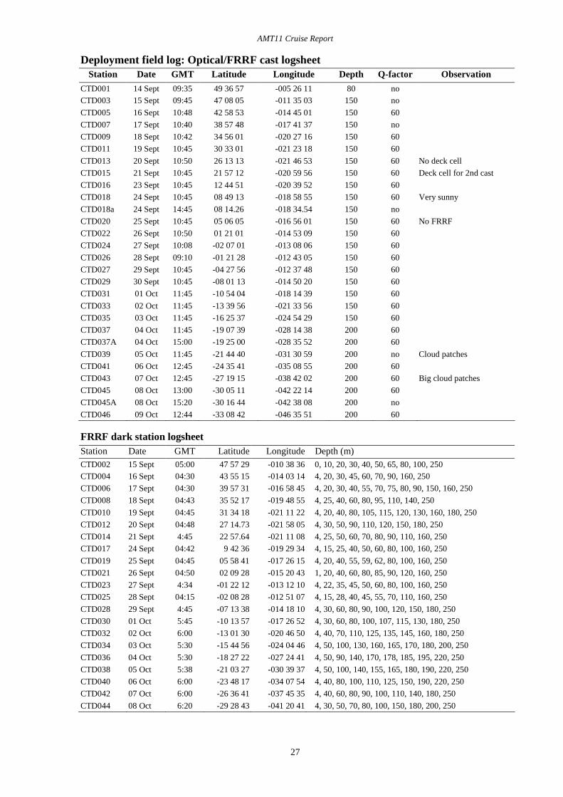
Deployment field log: Optical/FRRF cast logsheet Station Date GMT Latitude Longitude Depth Q-factor Observation

CTD001 14 Sept 09:35 49 36 57 -005 26 11 80 no CTD003 15 Sept 09:45 47 08 05 -011 35 03 150 no CTD005 16 Sept 10:48 42 58 53 -014 45 01 150 60 CTD007 17 Sept 10:40 38 57 48 -017 41 37 150 no CTD009 18 Sept 10:42 34 56 01 -020 27 16 150 60 CTD011 19 Sept 10:45 30 33 01 -021 23 18 150 60 CTD013 20 Sept 10:50 26 13 13 -021 46 53 150 60 No deck cell CTD015 21 Sept 10:45 21 57 12 -020 59 56 150 60 Deck cell for 2nd cast CTD016 23 Sept 10:45 12 44 51 -020 39 52 150 60 CTD018 24 Sept 10:45 08 49 13 -018 58 55 150 60 Very sunny CTD018a 24 Sept 14:45 08 14.26 -018 34.54 150 no CTD020 25 Sept 10:45 05 06 05 -016 56 01 150 60 No FRRF CTD022 26 Sept 10:50 01 21 01 -014 53 09 150 60 CTD024 27 Sept 10:08 -02 07 01 -013 08 06 150 60 CTD026 28 Sept 09:10 -01 21 28 -012 43 05 150 60 CTD027 29 Sept 10:45 -04 27 56 -012 37 48 150 60 CTD029 30 Sept 10:45 -08 01 13 -014 50 20 150 60 CTD031 01 Oct 11:45 -10 54 04 -018 14 39 150 60 CTD033 02 Oct 11:45 -13 39 56 -021 33 56 150 60 CTD035 03 Oct 11:45 -16 25 37 -024 54 29 150 60 CTD037 04 Oct 11:45 -19 07 39 -028 14 38 200 60 CTD037A 04 Oct 15:00 -19 25 00 -028 35 52 200 60 CTD039 05 Oct 11:45 -21 44 40 -031 30 59 200 no Cloud patches CTD041 06 Oct 12:45 -24 35 41 -035 08 55 200 60 CTD043 07 Oct 12:45 -27 19 15 -038 42 02 200 60 Big cloud patches CTD045 08 Oct 13:00 -30 05 11 -042 22 14 200 60 CTD045A 08 Oct 15:20 -30 16 44 -042 38 08 200 no CTD046 09 Oct 12:44 -33 08 42 -046 35 51 200 60

FRRF dark station logsheet Station Date GMT Latitude Longitude Depth (m) CTD002 15 Sept 05:00 47 57 29 -010 38 36 0, 10, 20, 30, 40, 50, 65, 80, 100, 250 CTD004 16 Sept 04:30 43 55 15 -014 03 14 4, 20, 30, 45, 60, 70, 90, 160, 250 CTD006 17 Sept 04:30 39 57 31 -016 58 45 4, 20, 30, 40, 55, 70, 75, 80, 90, 150, 160, 250 CTD008 18 Sept 04:43 35 52 17 -019 48 55 4, 25, 40, 60, 80, 95, 110, 140, 250 CTD010 19 Sept 04:45 31 34 18 -021 11 22 4, 20, 40, 80, 105, 115, 120, 130, 160, 180, 250 CTD012 20 Sept 04:48 27 14.73 -021 58 05 4, 30, 50, 90, 110, 120, 150, 180, 250 CTD014 21 Sept 4:45 22 57.64 -021 11 08 4, 25, 50, 60, 70, 80, 90, 110, 160, 250 CTD017 24 Sept 04:42 9 42 36 -019 29 34 4, 15, 25, 40, 50, 60, 80, 100, 160, 250 CTD019 25 Sept 04:45 05 58 41 -017 26 15 4, 20, 40, 55, 59, 62, 80, 100, 160, 250 CTD021 26 Sept 04:50 02 09 28 -015 20 43 1, 20, 40, 60, 80, 85, 90, 120, 160, 250 CTD023 27 Sept 4:34 -01 22 12 -013 12 10 4, 22, 35, 45, 50, 60, 80, 100, 160, 250 CTD025 28 Sept 04:15 -02 08 28 -012 51 07 4, 15, 28, 40, 45, 55, 70, 110, 160, 250 CTD028 29 Sept 4:45 -07 13 38 -014 18 10 4, 30, 60, 80, 90, 100, 120, 150, 180, 250 CTD030 01 Oct 5:45 -10 13 57 -017 26 52 4, 30, 60, 80, 100, 107, 115, 130, 180, 250 CTD032 02 Oct 6:00 -13 01 30 -020 46 50 4, 40, 70, 110, 125, 135, 145, 160, 180, 250 CTD034 03 Oct 5:30 -15 44 56 -024 04 46 4, 50, 100, 130, 160, 165, 170, 180, 200, 250 CTD036 04 Oct 5:30 -18 27 22 -027 24 41 4, 50, 90, 140, 170, 178, 185, 195, 220, 250 CTD038 05 Oct 5:38 -21 03 27 -030 39 37 4, 50, 100, 140, 155, 165, 180, 190, 220, 250 CTD040 06 Oct 6:00 -23 48 17 -034 07 54 4, 40, 80, 100, 110, 125, 150, 190, 220, 250 CTD042 07 Oct 6:00 -26 36 41 -037 45 35 4, 40, 60, 80, 90, 100, 110, 140, 180, 250 CTD044 08 Oct 6:20 -29 28 43 -041 20 41 4, 30, 50, 70, 80, 100, 150, 180, 200, 250

AMT11 Cruise Report

28

FRRF Underway log Start Finish

SDY Time (loc)

Time GMT Lat (N)

Lon (W) SDY

Time (loc)

Time GMT Lat (N)

Lon (W) File Name

258 12:15 11:15 4933.48 543.75 259 05:10 04:10 4757.47 1030.5 A11UW01 259 06:01 05:01 4757.15 1039.16 259 10:23 09:23 4710.8 1132.39 A11UW02 259 10:43 09:43 4705.39 1137.74 260 04:30 04:30 4355.26 1403.27 A11UW03 260 05:00 05:00 4354.05 1403.94 260 10:42 10:42 4258.03 1445.27 A11UW04 260 12:05 12:05 4252.68 1449.05 261 04:22 04:22 3957.3 1658.7 A11UW05 261 05:08 05:08 3957.54 1658.76 261 10:40 10:40 3857.61 1741.71 A11UW06 261 11:28 11:28 3856.33 1742.4 262 04:40 04:40 3552.26 1948.86 A11UW07 262 05:30 05:30 3551.35 1949.63 262 10:40 10:40 3455.78 2027.23 A11UW08 262 11:27 11:27 3454.48 2028.58 263 10:40 10:40 3032.93 2123.17 A11UW09 263 11:27 11:27 3031.34 2123.89 264 04:43 04:43 2714.72 2158.09 A11UW10 264 05:13 05:13 2714.58 2158.14 264 10:38 10:38 2613.23 2147.06 A11UW11 264 11:28 11:28 2611.89 2147.05 265 04:40 04:40 2257.49 2111.11 A11UW12 265 05:20 05:20 2257.63 2111.24 265 10:42 10:42 2157.15 2100.01 A11UW13 265 11:33 11:33 2154.84 2059.93 266 11:10 11:10 1728.3 2039.86 A11UW14 266 11:10 11:10 1728.26 2039.86 267 10:40 10:40 1244.52 2039.87 A11UW15 267 12:10 12:10 1235.78 2039.73 268 10:40 10:40 848.83 1859.16 A11UW16 268 11:25 11:25 848.4 1858.44 269 10:40 10:40 505.69 1656.11 A11UW17 269 11:30 11:30 505.16 1655.36 270 10:42 10:42 120.98 1453.14 A11UW18 270 11:25 11:25 120.72 1452.63 271 09:37 09:37 -206.68 1307.94 A11UW19 271 10:33 10:33 -207.25 1308.35 272 09:32 09:32 -121.65 1243.31 A11UW20 272 10:28 10:28 -124.58 1243.01 273 10:40 10:40 -428.16 1237.55 A11UW21 273 11:30 11:30 -428.9 1239.11 274 10:39 10:39 -801.4 1450.15 A11UW22 274 11:25 11:25 -801.77 1451.11 275 10:40 11:40 -1054.05 1814.7 A11UW23 275 11:25 12:25 -1054.48 1815.61 276 10:40 11:40 -1339.91 2133.97 A11UW24 276 11:29 12:29 -1340.22 2135.21 277 10:39 11:39 -1625.58 2454.56 A11UW25 277 11:26 12:26 -1625.58 2454.81 278 10:37 11:37 -1907.72 2814.28 A11UW26 278 11:21 12:21 -1907.81 2814.79 279 10:39 11:39 -2144.87 3130.77 A11UW27 279 11:28 12:28 -2145.89 3132.3 280 10:39 12:39 -2435.8 3508.74 A11UW28 280 11:33 13:33 -2436.97 3509.78 281 10:37 12:37 -2719.11 3841.66 A11UW29 281 11:28 12:28 -2719.25 3842.28 282 10:36 12:36 -3004.23 4221.12 A11UW30 282 11:34 13:34 -3005.17 4221.89 283 07:33 10:33 -3307.31 5022.1 A11UW31

AMT11 Cruise Report

29

Seawater Filtrations

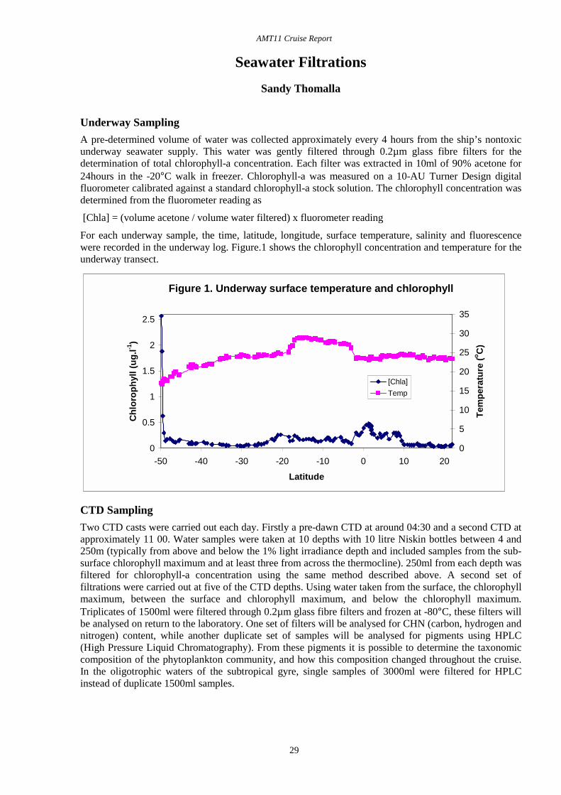
Sandy Thomalla Underway Sampling A pre-determined volume of water was collected approximately every 4 hours from the ship’s nontoxic underway seawater supply. This water was gently filtered through 0.2µm glass fibre filters for the determination of total chlorophyll-a concentration. Each filter was extracted in 10ml of 90% acetone for 24hours in the -20°C walk in freezer. Chlorophyll-a was measured on a 10-AU Turner Design digital fluorometer calibrated against a standard chlorophyll-a stock solution. The chlorophyll concentration was determined from the fluorometer reading as

[Chla] = (volume acetone / volume water filtered) x fluorometer reading

For each underway sample, the time, latitude, longitude, surface temperature, salinity and fluorescence were recorded in the underway log. Figure.1 shows the chlorophyll concentration and temperature for the underway transect.

Figure 1. Underway surface temperature and chlorophyll

0

0.5

1

1.5

2

2.5

-50 -40 -30 -20 -10 0 10 20

Latitude

Chl

orop

hyll

(ug.

l-1)

0

5

10

15

20

25

30

35

Tem

pera

ture

(o C)

[Chla]Temp

CTD Sampling Two CTD casts were carried out each day. Firstly a pre-dawn CTD at around 04:30 and a second CTD at approximately 11 00. Water samples were taken at 10 depths with 10 litre Niskin bottles between 4 and 250m (typically from above and below the 1% light irradiance depth and included samples from the sub-surface chlorophyll maximum and at least three from across the thermocline). 250ml from each depth was filtered for chlorophyll-a concentration using the same method described above. A second set of filtrations were carried out at five of the CTD depths. Using water taken from the surface, the chlorophyll maximum, between the surface and chlorophyll maximum, and below the chlorophyll maximum. Triplicates of 1500ml were filtered through 0.2µm glass fibre filters and frozen at -80°C, these filters will be analysed on return to the laboratory. One set of filters will be analysed for CHN (carbon, hydrogen and nitrogen) content, while another duplicate set of samples will be analysed for pigments using HPLC (High Pressure Liquid Chromatography). From these pigments it is possible to determine the taxonomic composition of the phytoplankton community, and how this composition changed throughout the cruise. In the oligotrophic waters of the subtropical gyre, single samples of 3000ml were filtered for HPLC instead of duplicate 1500ml samples.

AMT11 Cruise Report

30

Nitrogen uptake and regeneration

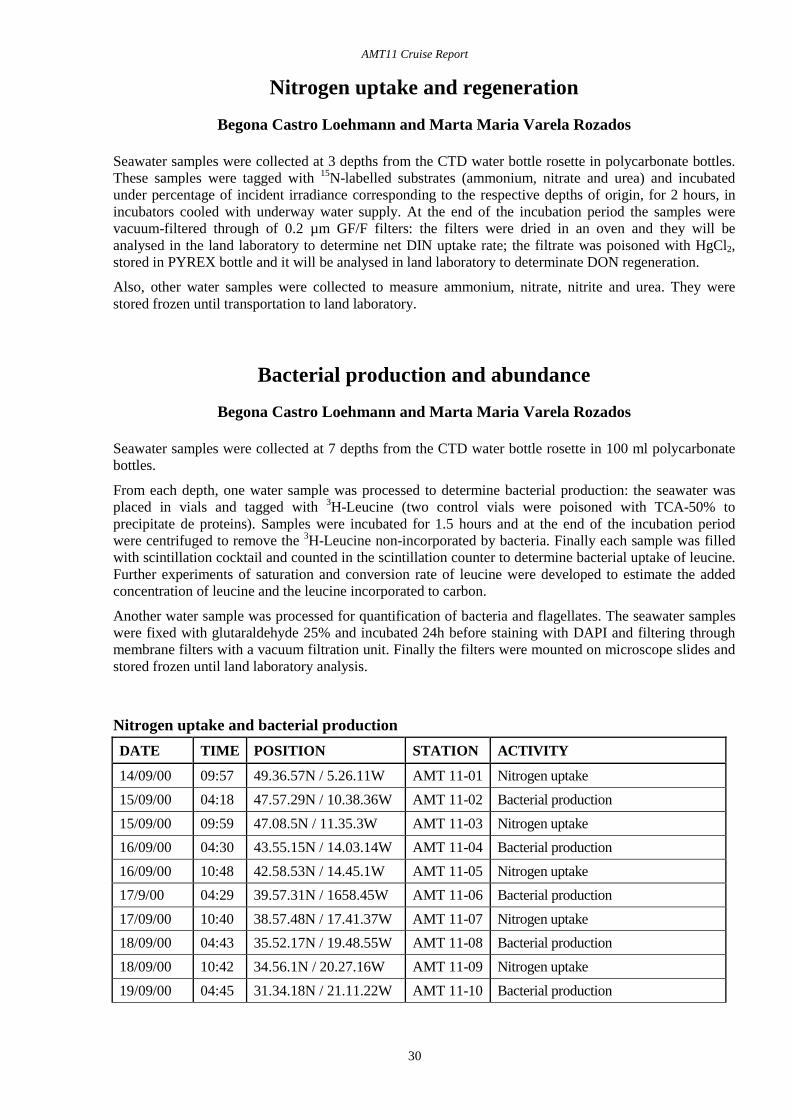
Begona Castro Loehmann and Marta Maria Varela Rozados Seawater samples were collected at 3 depths from the CTD water bottle rosette in polycarbonate bottles. These samples were tagged with 15N-labelled substrates (ammonium, nitrate and urea) and incubated under percentage of incident irradiance corresponding to the respective depths of origin, for 2 hours, in incubators cooled with underway water supply. At the end of the incubation period the samples were vacuum-filtered through of 0.2 µm GF/F filters: the filters were dried in an oven and they will be analysed in the land laboratory to determine net DIN uptake rate; the filtrate was poisoned with HgCl2, stored in PYREX bottle and it will be analysed in land laboratory to determinate DON regeneration.

Also, other water samples were collected to measure ammonium, nitrate, nitrite and urea. They were stored frozen until transportation to land laboratory.

Bacterial production and abundance Begona Castro Loehmann and Marta Maria Varela Rozados

Seawater samples were collected at 7 depths from the CTD water bottle rosette in 100 ml polycarbonate bottles.

From each depth, one water sample was processed to determine bacterial production: the seawater was placed in vials and tagged with 3H-Leucine (two control vials were poisoned with TCA-50% to precipitate de proteins). Samples were incubated for 1.5 hours and at the end of the incubation period were centrifuged to remove the 3H-Leucine non-incorporated by bacteria. Finally each sample was filled with scintillation cocktail and counted in the scintillation counter to determine bacterial uptake of leucine. Further experiments of saturation and conversion rate of leucine were developed to estimate the added concentration of leucine and the leucine incorporated to carbon.

Another water sample was processed for quantification of bacteria and flagellates. The seawater samples were fixed with glutaraldehyde 25% and incubated 24h before staining with DAPI and filtering through membrane filters with a vacuum filtration unit. Finally the filters were mounted on microscope slides and stored frozen until land laboratory analysis.

Nitrogen uptake and bacterial production DATE TIME POSITION STATION ACTIVITY

14/09/00 09:57 49.36.57N / 5.26.11W AMT 11-01 Nitrogen uptake 15/09/00 04:18 47.57.29N / 10.38.36W AMT 11-02 Bacterial production 15/09/00 09:59 47.08.5N / 11.35.3W AMT 11-03 Nitrogen uptake 16/09/00 04:30 43.55.15N / 14.03.14W AMT 11-04 Bacterial production 16/09/00 10:48 42.58.53N / 14.45.1W AMT 11-05 Nitrogen uptake 17/9/00 04:29 39.57.31N / 1658.45W AMT 11-06 Bacterial production 17/09/00 10:40 38.57.48N / 17.41.37W AMT 11-07 Nitrogen uptake 18/09/00 04:43 35.52.17N / 19.48.55W AMT 11-08 Bacterial production 18/09/00 10:42 34.56.1N / 20.27.16W AMT 11-09 Nitrogen uptake 19/09/00 04:45 31.34.18N / 21.11.22W AMT 11-10 Bacterial production

AMT11 Cruise Report

31

DATE TIME POSITION STATION ACTIVITY

19/09/00 10:45 30.33.1N / 21.23.18W AMT 11-11 Nitrogen uptake 20/09/00 04:45 27.14.43N / 21.58.5W AMT 11-12 Bacterial production 20/09/00 10:45 26.13.13N / 21.46.53W AMT 11-13 Nitrogen uptake, Bacterial production 21/09/00 04:45 22.57.34N / 21.11.01W AMT 11-14 Bacterial production 21/09/00 10:45 21.57.12N / 20.59.56W AMT 11-15 Nitrogen uptake, Bacterial production 23/9/00 10:45 12.44.51N / 20.39.52W AMT 11-16 Nitrogen uptake, Bacterial production 24/9/00 4.45 09.42.25N / 19.29.22W AMT 11-17 Bacterial production 24/9/00 10:45 08.49.13N / 18.58.55W AMT 11-18 Nitrogen uptake, Bacterial production 25/9/00 04:45 05.58.41N / 17.26.15W AMT 11-19 Bacterial production 25/9/00 10:45 05.06.05N / 16.56.1W AMT 11-20 Nitrogen uptake, Bacterial production 26/9/00 04:50 02.09.28N / 15.20.43W AMT 11-21 Bacterial production 26/9/00 10:50 01.21.01N / 14.53.09W AMT 11-22 Nitrogen uptake, Bacterial production 27/9/00 4.34 01.22.12S / 13.12.10W AMT 11-23 Bacterial production 27/9/00 10:08 02.07.01S / 13.08.06W AMT 11-24 Nitrogen uptake, Bacterial production 28/9/00 04:05 02.08.28S / 12.51.07W AMT 11-25 Bacterial production 28/9/00 09:35 01.21.28S / 12.43.05W AMT 11-26 Nitrogen uptake, Bacterial production 29/9/00 10:45 04.2756S / 12.37.48W AMT 11-27 Nitrogen uptake, Bacterial production 30/9/00 04:45 07.13.38S / 14.18.10W AMT 11-28 Bacterial production 30/9/00 10:45 08.01.13S / 14.50.20W AMT 11-29 Nitrogen uptake, Bacterial production 10/01/2000 05:45 10.13.57S / 17.26.52W AMT 11-30 Bacterial production 10/01/2000 11:45 10.54.4S / 18.1439W AMT 11-31 Nitrogen uptake, Bacterial production 10/02/2000 05:45 13.01.30S / 20.46.50W AMT 11-32 Bacterial production 10/02/2000 11:45 13.39.56S / 21.33.56W AMT 11-33 Nitrogen uptake, Bacterial production 10/03/2000 05:30 15.44.56S / 24.04.46W AMT 11-34 Bacterial production 10/03/2000 11:45 16.25.37S / 24.54.29W AMT 11-35 Nitrogen uptake, Bacterial production 10/04/2000 05:30 18.27.22S / 27.24.41W AMT 11-36 Bacterial production 10/04/2000 11:45 19.07.39S / 28.14.38W AMT 11-37 Nitrogen uptake, Bacterial production 10/05/2000 05:30 21.03.27S / 30.39.37W AMT 11-38 Bacterial production 10/05/2000 11:45 21.44.40S / 31.30.59W AMT 11-39 Nitrogen uptake, Bacterial production 10/06/2000 06:00 23.48.17S / 34.07.54W AMT 11-40 Bacterial production 10/06/2000 12:45 24.35.41S / 35.08.55W AMT 11-41 Nitrogen uptake, Bacterial production 10/07/2000 06:00 26:36.41S / 37.45.35W AMT 11-42 Bacterial production 10/07/2000 12:45 27.19.15S / 38.42.02W AMT 11-43 Nitrogen uptake, Bacterial production 10/08/2000 06:15 29.18.43S / 41.20.41W AMT 11-44 Bacterial production 10/08/2000 13:00 30.05.11S / 42.22.14W AMT 11-45 Nitrogen uptake, Bacterial production 10/09/2000 12:44 33.08.42S / 46.35.51W AMT 11-46 Nitrogen uptake, Bacterial production

AMT11 Cruise Report

32

Phytoplankton-mediated carbon and oxygen flows

Emilio Fernández, Ramiro Varela, Pablo Serret Universidad de Vigo (Spain)

Size-fractionated chlorophyll a and primary production From each CTD cast, seawater samples (300 cm3) were drawn from 5-6 selected depths and filtered sequentially through 0.2, 2 and 20 µm polycarbonate filters which were immediately placed in glass vials and 8 ml of 90% added. After extraction at –20 ºC for ca. 20 h, chlorophyll a fluorescence was measured with a Turner Designs 10-AU fluorometer.

For the measurement of size-fractionated primary production rates four 70 cm3 acid-cleaned polypropylene bottles (3 transparent + 1 dark) were filled with water from 5 depths at every early morning CTD cast. Each bottle was inoculated with 333 to 814 kBq (9-22 to µCi) NaH14CO3, depending on the biomass of primary producers, as to yield activities exceeding 3000 dpm. Samples were incubated at dawn in an on-deck incubator at irradiances corresponding approximately to those experienced by the cells at the sampling depths. Incubations lasted 24 h. Samples were then filtered at very low vacuum pressure (< 50 mm Hg) through a cascade of 20, 2 and 0.2 µm polycarbonate filters. Filters were decontaminated by exposure to fumes of concentrated HCl fumes for 20-22 h and placed in plastic scintillation vials and 3 ml of Ultima GOLD XR LSC scintillation cocktail added to each vial. The radioactive activity in the filters was determined with a Beckman LS600SC liquid scintillation counter onboard. Quenching corrections were performed using internal quench correction.

The highest rates of primary production rates during AMT-11 were found at the equatorial region between 10 ºN and 10º S, with maximum values found at shallow subsurface (20-40 m depth) layers where > 15 mg C m-3 d-1 were measured. Primary production rates in the subtropical gyres were extremely low (< 3 mg C m-3 d-1 ) in the whole water column. Relatively high carbon incorporation rates by phytoplankton were measured at temperate and tropical North Atlantic waters.

-40 -30 -20 -10 0 10 20

Latitude

Total primary production (mg m-3 d-1)

-160

-140

-120

-100

-80

-60

-40

-20

Depth (m

)

1

2

3

4

6

8

10

15

AMT11 Cruise Report

33

Carbon incorporation into photosynthetic products Samples for the determination of the rates of photosynthetic carbon incorporation into low molecular weight metabolites, lipids, polysaccharides and proteins were collected at the same stations and from the same depths where size-fractionated primary production rates was measured. Each bottle was inoculated with 333 to 814 kBq (9-22 to µCi) NaH14CO3 depending on the biomass of primary producers as to yield activities exceeding 3000 dpm. Samples were incubated at dawn in an on-deck incubator at irradiances corresponding approximately to those experienced by the cells at the sampling depths. Incubations lasted 24 h. Samples were then filtered at very low vacuum pressure (< 50 mm Hg) through Millipore GFF filters which were kept frozen at –80 ºC until further analysis ashore.

Photosynthesis-irradiance (P-I) curves The relationship between irradiance and the rate of carbon incorporation by phytoplankton was evaluated at 3 depths every late-morning station, 3 different depths down to the deep chlorophyll maximum. 13 Corning bottles were filled from each depth, inoculated with 333 to 814 kBq (9-22 to µCi) NaH14CO3 and incubated with halogen near solar lamps for approximately 2 hours. The incubators were cooled with near sea-surface water (18.5-23ºC). The PAR irradiance (µE m-2 s-1) of each incubator cell (corresponding to the light each Corning bottle is about to receive) was measured before every incubation with a LI-COR 1000 quantometer equipped with a LI-COR plate sensor. The last Corning bottle from each depth was protected against light with aluminium foil and used as a dark reference. After the incubation time, samples were removed from the incubator and filtered through Millipore GF/F filters, which were processed as described above for the determination of size-fractionated primary production rates.

Total particulate matter absorption spectra Total particulate matter absorption spectra were measured on GFF filters fitted with an opal glass on a single beam Beckman DU650 scanning (350-750 nm) spectrophotometer. 1.5 to 3 ml of seawater were filtered through Millipore GFF glass fibre filter and a modified opal-glass technique was used to determine the optical density OD(λ) of the particles retained on the filter. An identical glass fibre filter soaked in filtered seawater was used as a blank. The optical density at 750 nm was subtracted from OD(λ) and the phytoplankton absorption coefficients ap(λ) were estimated according to the relationship:

ap =2.3 ⋅OD λ( )⋅s

V ⋅β λ( )

where V is the volume of filtered seawater, s the filtering area of the GF/F filter and the beta factor β(λ) was estimated as:

( ) ( )β λ λ= ⋅ −163 0 22. .OD The light absorption by particulate detritus ad(λ) was estimated numerically following the method of Bricaud and Strawski (1990) improved for low detritus content (Varela et. al. 1998).

References BRICAUD, A., and D. STRAMSKI. 1990. Spectral absorption coefficients of living phytoplankton and nonalgal biogenous matter: A comparison between the Peru upwelling area and the Sargasso Sea. Limnol. Oceanogr. 35: 562-582.

VARELA, R.A..; FIGUEIRAS, F.; AGUSTÍ, S. and B. ARBONES 1998 Determining the contribution of pigments and the non-algal fraction to total absorption: toward a global algorithm. Limnol. Oceanogr ., 43(3) :449-457

Rates of O2 production and consumption Gross production (GP), net community production (NCP) and dark community respiration (DCR) were determined from in vitro changes in dissolved oxygen. At each early morning station, 125 cm3

AMT11 Cruise Report

34

borosilicate glass bottles were filled from 5-6 depths. From each depth, five zero time replicates were fixed immediately, and a further ten replicate bottles were incubated in surface water cooled light and dark deck incubators for 24 hours. Light incubators were covered with polycarbonate screens incorporating neutral density acrylic of differing transmission to give a range of irradiances which simulated those experienced by the cells in their original environment. The dark incubators were covered with opaque screens. Production and respiration rates were calculated from the difference between the means of the replicate light and dark incubated and zero time analyses.

Microplankton nets Vertical hauls (100 m) were carried out with a 20 µm microplankton net at every mid morning station. The sample was transferred to a 250 ml measuring cylinder and divided into 2 aliquots. A 100 ml subsample was placed in a glass bottle and fixed with buffered formalin for the further quantification ashore of the biomass of microplankton species by image analysis of the biomass. 25 to 100 ml of the remaining sample was filtered through a Millipore GFF filter and kept frozen (-80 ºC) for the further determination of particulate C and N concentration ashore.

Station Size-fractionated Chlorophyll a

Size-fractionated PP

Carbon incorporation

P-I curves POM absorption spectra

O2 production and consumption

Microplankton nets

11-1 X 11-2 X X X X 11-3 X X X 11-4 X X X X 11-5 X X X X 11-6 X X X X 11-7 X X X X 11-8 X X X X 11-9 X X X X 11-10 X X X X 11-11 X X X X 11-12 X X X X 11-13 X X X X 11-14 X X X X 11-15 X X X X 11-16 X X X X 11-17 X X X X 11-18 X X X X 11-19 X X X X 11-20 X X X X 11-21 X X X X 11-22 X X X X 11-23 X X X X 11-24 X X X X 11-25 X X X X 11-26 X X X X 11-27 X X X X 11-28 X X X X 11-29 X X X X 11-30 X X X X 11-31 X X X X 11-32 X X X X 11-33 X X X X 11-34 X X X X 11-35 X X X X 11-36 X X X X 11-37 X X X X 11-38 X X X X 11-39 X X X X 11-40 X X X X 11-41 X X X X 11-42 X X X X 11-43 X X X X 11-44 X X X X 11-45 X X X X

AMT11 Cruise Report

35

Macro-nutrient depth profiles - CDOM depth profiles

Vassilis Kitidis

Scientific rationale The purpose of this work is to study the concentration dynamics of macro-nutrients and chromophoric dissolved organic matter (CDOM) in the top 250 metres along the cruise transect as it crosses distinct, contrasting biogeographical regions. These data add to the AMT time series and form part of the core research programmes of PML/CCMS.

Samples were collected daily from vertical CTD casts and analysed for the concentrations of plant macro-nutrients, nitrate (NO3

-), nitrite (NO2-), ammonium (NH4

+) phosphate (PO43-) ions and silicate (SiO2).

These macro-nutrients are essential for phytoplankton growth and usually depleted in the mixed layer, in oceanic environments, due to their uptake by primary producers. A sharp increase in the macro-nutrient concentrations is found below the mixed layer. As phytoplankton growth is nutrient limited in the upper mixed layer (UML), and light limited below, primary producers concentrate near the pycnocline that separates the UML from the water below. This ensures optimal growth in the nutrients vs. light availability trade-off. Biological activity acts as a source of organic matter (particulate and dissolved), while the pycnocline forms a physical barrier for organics which are aggregated and thereby support local bacterial populations at the pycnocline. The re-mineralisation of organic matter is evident from the ammonium and nitrite concentration profiles which peak below the pycnocline and chlorophyll maximum. Ammonium ion is produced in the excreta of the biota and from ‘sloppy-feeding’ of zooplankton on phytoplankton. Nitrite is produced as an intermediate product of nitrification the conversion of ammonium to nitrite, by nitrifying bacteria. A typical profile of these three inorganic nitrogen species is shown in figure 1. Note the succession of ammonium peak to nitrite peak to high nitrate with increasing depth.

N - species vs. Z, AMT 11, CTD 03 (47.14oN, 11.59oW)

0

50

100

150

200

250

0 2 4 6 8

[Nitrate] /10-6M

Z /m

0 0.1 0.2 0.3 0.4

[Nitrite],[Ammonium] /10-6M

Nitrate

Nitrite

Ammonium

Figure 1. Depth profile of nitrite, nitrate and ammonium ions from station 03 (47.14oN, 11.59oW) of AMT11 research cruise. Ammonium (empty circles) concentration, peaks at approximately 70m depth as a result of biological excretion. This is converted to nitrite and subsequently nitrate, by nitrifying bacteria. This succession is visible from the distribution of nitrite (black circles) concentration which peaks just below and ammonium and finally the nitrate (grey circles) nutricline, below. Regions of differing nutrient regimes and biogeochemistry are highlighted in figure two. This is a compilation of data from the first 18 stations. A progression can be seen as one moves from north to south along the cruise-track. The fairly mixed water column at the shelf edge, off the higher latitudes, is succeeded by a stratified system with a nutricline which becomes progressively deeper as the cruise track transects the edge of the oligotrophic-north-Atlantic gyre. This is followed by the upwelling regions, off

AMT11 Cruise Report

36

the coasts of west-Africa, where the highest concentrations are encountered and the UML becomes shallower again. This area is far more productive, something that was apparent from the increased biological activity in the water during stations.

Nitrate /E-6 M

AMT 11, Nitrate distribution with latitude and depth along cruise track (Stations 1-18)

10.00 15.00 20.00 25.00 30.00 35.00 40.00 45.00

Latitude

-250.00

-200.00

-150.00

-100.00

-50.00

0.00

Dep

th /m

0.05

2.05

4.05

6.05

10.05

14.05

18.05

22.05

28.05

Figure 2: The distribution of nitrate along the AMT 11 cruise track with northern latitude and depth. Dots represent data points. Note the low concentrations in the nutrient depleted UML, followed by a sharp increase in concentration with depth (nutricline). Contrasting biogeochemical regions here are the edge of the north-Atlantic gyre (between 27o-40o N) with a deep UML and the lowest concentrations and the west-African upwelling regions (between 8o-25o N) with a shallower UML and sharp nutricline. Depth profiles of chromophoric dissolved organic matter (CDOM) are of importance to ocean optics and remote sensing. CDOM absorption spectra provide some information on the source of the material, allowing to distinguish ‘old’ material from deeper waters, ‘fresh’ material from the chlorophyll maximum and photodegraded material from surface waters. As with macro-nutrients, distribution of CDOM along the cruise transect is of particular interest between the different biogeochemical provinces. This work was also carried out on AMT 9 (JR 45) and AMT 10 (JR 49), thus the data will collected on the present cruise will complement the set already available.

Analytical Macro-nutrient analysis was carried out using air-segmented-flow, colorimetric techniques, with a Technicon Autoanalyzer II. For the determination of ammonium ion concentrations, a nanomolar sensitivity, fluorometric method was used. Samples for nutrient analysis were collected in 60 ml HDPE (Nalgene) bottles and analysed immediately after collection. Samples for spectrophotometric analysis were collected in 200 ml analytical grade glass, volumetric flasks. Absorption spectra were taken with a Shimadzu double beam UV/visible spectrophotometer, using 10 cm path length optically paired cuvettes. Samples were also pressure filtered through 0.7 µm filters (Whatman, GF/F), but filtering introduced precision errors and was therefore abandoned. The absorption coefficient at 350 nm and spectral slope of the decay between 290 and 350 nm are used as measures of concentration and origin respectively.

AMT11 Cruise Report

37

AutoFlux Trials

Margaret J. Yelland and Robin W. Pascal

This report describes the work undertaken on the “AutoFlux” system by SOC staff on the RRS James Clark Ross during the U.K. to Falklands passage between 11 September and 17 October 2000. This work coincided with the Atlantic Meridional Transect (AMT) 11 cruise (JR52) which ended on 11 October 2000, and is described elsewhere (Woodward, 2000). The SOC presence on the ship was sponsored by John King (BAS) as part of his Q3 (Antarctic Climate Processes) science program.

The aim of the cruise was to test and develop the AutoFlux air-sea interaction system and its associated prototype instrumentation. The system is intended to provide real-time air-sea fluxes of momentum, sensible heat, latent heat and CO2, in addition to the usual mean meteorological parameters. The fluxes are calculated via the “inertial dissipation” method (Yelland et al., 1998), using data from various fast-response instruments. Most of the instruments used in the system have been well proved during SOC research cruises over the last 10 years or more, but the dedicated sonic temperature sensor and the infra-red H2O/CO2 sensor are prototype instruments developed by colleagues involved in the AutoFlux project (MAST project MAS3-CT97-0108). Likewise, the logging and processing system is itself based on software systems which have been developed at SOC/IOS since the 1980s, but many aspects of the system are new and were tested and developed further during the cruise. By the fourth week of the cruise the system was automatically producing hourly direct measurements of the air-sea fluxes and was sending summary messages of the data back to SOC via the ORBCOMM satellite communications system in near real time.

Acknowledgements Thanks are due to the officers and crew of the RRS James Clark Ross, particularly the navigation officers for their diligence over the cloud observations, to John King (BAS) for sponsoring our presence on the ship, and to the AMT science team for making the SOC gatecrashers welcome on their cruise. We are also grateful to our AutoFlux colleagues who made the sonic temperature and the H2O/CO2 sensors available to us, as well as to Dave Hosom and Co. from Woods Hole Oceanographic Institute for the loan of their sea surface temperature system.

1. Introduction The Southampton Oceanography Centre’s JRD Meteorology Team took part in the U.K. to Falklands passage on the RRS James Clark Ross in order to trial the “AutoFlux” air-sea interaction system and its associated prototype instrumentation. The SOC presence on the cruise was sponsored by John King (BAS) as part of his Q3 science program. This work coincided with the Atlantic Meridional Transect (AMT) 11 cruise (JR52) which ended on 11 October 2000, and is described elsewhere (Woodward, 2000).

The AutoFlux system is intended to provide real-time air-sea fluxes of momentum, sensible heat, latent heat and CO2, in addition to the usual mean meteorological parameters (AutoFlux Group, 1996). The fluxes are calculated via the “inertial dissipation” method (Yelland et al., 1998), using data from various fast-response instruments. Most of the instruments used in the system have been well proved during SOC research cruises over the last 10 years or more, but the dedicated sonic temperature sensor (Gill Instruments Ltd.) and the infra-red H2O/CO2 sensor (Mierij Co. and the Royal Netherlands Meteorological Institute “KNMI”) are prototype instruments developed by colleagues involved in the AutoFlux project (MAST project MAS3-CT97-0108). In addition to these fast response prototype instruments, the cruise also provided an opportunity to test the Woods Hole Oceanographic Institute (WHOI) sea surface temperature system. The AutoFlux logging and processing system is itself based on software systems which have been developed at SOC/IOS since the 1980s, but many aspects of the system are new and were tested and developed further during the cruise.

The AutoFlux system was set up while the ship was still in Grimsby and logged data continuously from the time of departure (0400 GMT on 12 September, day 256). The ship called in to Portsmouth for about 12 hours (from 0700 to 1900 on day 257) and in to Montevideo for just over 2 days (from 1200 day 285

AMT11 Cruise Report

38

to 1900 day 287). The system was shut down on 16 October at 1500 GMT, about 20 hours before docking in Stanley. Figure 1 shows the ship track from Portsmouth to the point at which the system was shut down. A wide range of conditions were experienced; 1 minute averages of U10N varied from calm to 20 m/s with a mean of 7 m/s, sea surface temperatures varied from 5° to 30°, air temperatures from 5° to 30°, and the air-sea temperature difference ranged from –4° to 4°.

This report discusses the AutoFlux instrumentation (Section 2) and the AutoFlux logging system (Section 3). Data from the ship’s navigation and scientific instrumentation were also obtained (Section 4). Hourly visual cloud observations (Section 5) were also taken throughout the cruise as part of a separate SOC Meteorology Team study into the parameterisation of downwelling longwave radiation from Voluntary Observing Ship cloud observations. Section 6 describes the performance and reliability of the AutoFlux system and associated instrumentation. Section 7 discusses the initial comparisons made between the AutoFlux and ship data streams, and includes a “first look” at the longwave parameterisation (Section 7.2). Finally, Section 8 summarises the major AutoFlux system developments achieved during the cruise. All times in this report are given as GMT.

More information on air-sea fluxes and the AutoFlux project in particular can be found under; http://www.soc.soton.ac.uk/JRD/MET/AUTOFLUX

2. Instrumentation The SOC Meteorology Team instrumented the JCR with a variety of meteorological sensors, plus a GPS navigation system. The mean meteorological sensors (Table 1) measured air temperature and humidity, air pressure, sea surface temperature, incoming shortwave (300-3000 nm) radiation and incoming longwave (4-50 micron) radiation. The surface fluxes of momentum, heat, moisture and CO2 were obtained using the fast-response instruments in Table 2. The HS sonic anemometer provided mean wind speed and direction data in addition to the momentum flux estimates. The AutoFlux system also incorporates navigation instruments (Table 3) in order to obtain ship’s position and to correct the meteorological data for ship speed and heading.

The positions of the instruments are indicated in Figure 2. Most of the instruments were mounted on the ship’s foremast in order to obtain the best exposure. The psychrometers and the fast response sensors were all located on the foremast platform and the radiation sensors were mounted on the “bird table” at the top of the foremast extension. The heights relative to the ship’s waterline of the instruments on the foremast platform were; HS sonic anemometer, 15.75 m; psychrometers. 15.40 m; sonic temperature sensor, 15.75 m (both positions); IFM H2O/CO2 sensor 15.55 m (first position) and 15.30 m (second position). The sonic temperature and the IFM sensors were both moved on day 277 at around 1200 GMT.

The sea surface temperature (SST) “soap” (thermistor) was trailed over the port side of the ship (not the starboard as illustrated). The Woods Hole hull contact SST sensor was located in the void space next to the transducer space on the starboard side of the ship, about 3.5 m below the water line.

AMT11 Cruise Report

39

Sensor Channel, variable name

Address serial no. Calibration

Y = C0 + C1*X + C2*X2 + C3*X3

Sensor position Parameter

(accuracy)

Psychrometer

1

pds2

$ARD

IO2002 DRY

C0 -10.10419

C1 3.687167e-2

C2 4.437374 e-6

C3 -1.244586-10

Psychrometer 2

pws2

$ERD IO2002 WET C0 -10.15374

C1 3.847717-2

C2 2.047162-6

C3 -1.487345-10

Foremast platform. To stbd of HS

sonic.

wet- and dry-bulb air temperatures,

and humidity

(0.05º)

Psychrometer 3

pdp1

$VRD IO2003 DRY C0 -10.27104

C1 3.757243 e-2

C2 3.514678-6

C3 -8.593494-10

Psychrometer 4

pwp1

$WRD IO2003 WET C0 -10.11169

C1 3.79443e-2

C2 3.070856 -6

C3 -6.940979-10

Foremast platform.

To port of HS sonic.

wet- and dry-bulb air temperatures,

and humidity

(0.05º)

SST “soap”

to day 269 10:50

5

soap SST

$XRD PD0002/52 C0 70.01189

C1 -0.1188988

C2 1.404794e-4

C3 -1.003271e-7

Over port side of foredeck

sea surface temperature

(0.1º)

SST “soap”

from day 269 10:50

5

soap SST

$XRD PD0005/53 C0 71.34180732

C1 -0.127521707

C2 1.57588211e-4

C3 -1.172824837e-7

Over port side of foredeck

sea surface temperature

(0.1º)

Eppley LW

Dome

6, Td1 $HRD 31170 C1 1

Body 7, Ts1 $QRD 31170 C1 1

Thermopile 8, E1 $2RD 31170 C1 1

foremast top

forwards position

incoming LW radiation

Eppley LW Dome

9, Td2 $BRD 27225 C1 1

Body 10, Ts2 $6RD 27225 C1 1

Thermopile 11, E2 $CRD 27225 C1 1

foremast top

aft position

incoming LW radiation

Kipp & Zonen SW

12

SWm

$1RD 27225 C1 1 foremast top, port side

incoming SW radiation

Vaisala Pressure

13

press

n/a ptb220 1 UIC air pressure

WHOI hull SST

sstMEAN

n/a

n/a

void space sea surface temp.

Table 1. The mean meteorological sensors. Left to right, the columns show; sensor type, channel number and variable name, rhopoint address, serial number of instrument, calibration applied, position on ship, and the parameter measured.

AMT11 Cruise Report

40

Sensor Program Location Data Rate Sections derived flux

Gill Horizontally Symmetrical Research Ultrasonic Anemometer

gillhs

Port side of

foremast platform

20 Hz

64

momentum and heat

Gill dedicated sonic temperature

sensor

stemphs

Port (to day 277 12:00) then stbd side of platform

20 Hz

64

heat

IFM IR H20/CO2 sensor

ifmhs

Port side of

foremast platform

10 Hz

32

H2O and

CO2

Table 2. The fast response sensors.

Instrument Acquisition program Position Sampling rate Parameters

CSI LGBX - PRO GPS receiver

gps6

aerial on aft rail of wheelhouse deck

1 or 0.5 Hz GPS time, lat, lon, sog, cog and QC information

KVH fluxgate compass

gps6 UIC lab 1 Hz ship’s heading (magnetic)

Table 3. The navigation instruments.

SST “soap”

GPS aerial

Radio meters

fore mastplatform

Figure 2a. Schematic of the instrument locations.

3. The AutoFlux logging system.

3.1 System management All the SOC instruments were logged via the AutoFlux system (Pascal et al., 2000). The exception to this was the WHOI hull sensor which was only received at SOC on the day of departure to the ship. The hull sensor was initially logged via a PC, but a UNIX management program was written and the sensor was integrated into the AutoFlux system on day 272. The AutoFlux system was based on one Unix workstation, named “southerly” (SO). A second identical workstation (“southeasterly”, SE) was used for system development. Both workstations were networked but were set up in stand-alone mode and not integrated into the ship’s system. Each workstation was cross-mounted with the other, allowing easy transfer of data and software between them and the sharing of devices installed on either station. Backups of both were performed weekly to CD (via the CD writer on SO) and exabyte (via the drive on SE). Table A1.1 (Appendix 1) lists the various modifications to the logging system that took place during the cruise.

The AutoFlux data acquisition system on SO ran multiple real time data acquisition and system programs, and this workstation was equipped with 8 extra serial ports for the multiple serial communications required. Both workstations had a variety of extra features, such as an auto-boot function and other

AMT11 Cruise Report

41

system software designed to make the data acquisition as robust and reliable as possible. These applications were;

Powerchute:- Both systems were attached to uninterruptible power supplies (UPSs) which were managed by UPS powerchute software. This monitors UPS loads, utility supply etc. and includes a background process which provides orderly shutdown of the host computer in the event of an extended AC power failure.

Program Monitor:- Runs the data acquisition programs and continues to monitor that they are currently active. If an acquisition program crashes it is automatically re-started and an indicator is set. As additional data analysis programs were written and implemented these were also managed by the Program Monitor.

Time Sync:- This program acquires time from the GPS receiver and adjusts the workstation time if the error is greater than 1 second. Jumps greater than 10 seconds are flagged and control is passed to the user before any adjustments are made.

3.2 Data acquisition Data were acquired continuously throughout the cruise using various logging programs on SO. These were;

“Gmet2” – This acquires the mean meteorological variables and was set up to sample the 13 channels of data listed in Table 1. Each sensor is attached to a Rhopoint module which converts the sensor output into digital data, and communicates it to the logging system via an RS485 network. The sensors were interrogated once every 10 seconds.

“Gillhs”, “stemphs” and “ifmhs” – These programs logged and processed data from the HS sonic anemometer, the sonic temperature sensor and the IFM fast-response H2O/CO2 sensor respectively. The programs are very similar. To take the HS sonic as an example, 64 sections of data were obtained every hour, each section consisting of 1024 data samples which are output from the anemometer at a rate of 20 Hz. At the end of the 64 sections the data are processed to produce spectra and quality control parameters. The different data rates of the three instruments and the number of sections obtained every hour are listed in Table 2.

“GPS6” - This managed the GPS differential navigation system and the fluxgate compass. Data were logged continuously at a rate of 1 Hz. This data rate was unnecessarily high and was reduced to 0.5 Hz on day 276.

“acm” - This was the UNIX management program written for the WHOI hull sensor. This sensor communicates data via two modems, one placed near the sensor and the other placed in the Gravimeter Room. The two modems communicate acoustically via the ship’s frame. From the Gravimeter Room the data were transmitted via the ship’s scientific wiring. To conserve battery life, the modems were sent to sleep for 10 minutes at a time and then interrogated for sea surface temperature data from the hull sensor, which returned three values on each interrogation.

3.3 Data processing and fluxes The following UNIX scripts were written during the cruise in order to process the data streams and produce the surface fluxes. These scripts utilise a suite of “pexec” FORTRAN programs. The scripts were managed by the CVI program “scp” which ran them hourly (except for “scrp.daily” which is run once a day).

“scrp.amet” – reads the calibrated mean meteorological data into a PEXEC file, applies basic quality control criteria and selects which psychrometer data to use. Also calculates the longwave radiation from the 3 channels output by the Epply sensors.

“scrp.anav” – reads the GPS and gyro information into a PEXEC file and converts heading and direction variables into north and east components prior to averaging.

“scrp.HULL” – reads the WHOI data into a PEXEC file and applies basic quality control criteria.

“scrp.HS” – reads the “*.mws” summary files from the HS sonic anemometer into a PEXEC file.

“scrp.IFM” - reads the “*.mws” summary files from the IFM sensor into a PEXEC file.

AMT11 Cruise Report

42

“scrp.STEMP” - reads the “*.mws” summary files from the sonic temperature sensor into a PEXEC file.

“scrp.flux” – merges the 6 separate data streams above into one file (averaging the mean meteorological and navigation data, and interpolating the WHOI SST data). If any data streams are absent they are replaced by dummy data files. Further quality control is applied and then true wind speed, true wind direction and surface fluxes are calculated.

“scrp.plot” – writes out an ASCII file of processed data, fluxes and quality control parameters for use in the AutoFlux display and the ORBCOMM message.

“scrp.daily” – appends the hourly files from each data stream and the hourly flux files into separate daily files which are moved to an archive directory. The previous day’s hourly files are then removed once the daily files have been created successfully.

4. Ship data streams Some of the ship’s data streams were logged for comparison with the AutoFlux data. These data streams were;

adcp (acoustic doppler current profiler - to correct wind speed relative to surface currents)

anemom (ship’s anemometer on the “bird table”)

dop_log (doppler log - to correct wind speed relative to surface currents)

em_log (electromagnetic log - to correct wind speed relative to surface currents)

gps_nmea (navigation stream - to check AutoFlux navigation system)

gyro (gyro compass - to check AutoFlux compass system)

oceanlog (thermosalinograph data plus air pressure and other mean met data)

CTD (temperature channels obtained in order to calibrate the other SST sensors)

Initial examination of the ship’s data streams showed that;

1) The adcp did not produce sensible data while the ship was underway, and the data did not improve sufficiently to be useful while on station.

2) The doppler log worked intermittently to start with and was then turned off.

3) The em log has yet to be examined, but, as it only measures one component of ship velocity relative to the water and there is a lack of comparison data due to the failure of the adcp and doppler log, it’s usefulness will be very limited.

4) The ship’s anemometer worked (Section 7.3)

5) The ship’s navigation data streams had no problems beyond initial time jumps when the ship’s clock was being set. The Level C time stamp occasionally produced time jumps around midnight due to rounding errors when converting between seconds and decimal jday. A comparison with the AutoFlux navigation data is given in Section 7.3.

6) The oceanlogger data were primarily logged for the sea surface temperature from the thermosalinograph (TSG) which will be discussed in Section 7.1 However, it was noticed that neither the PAR sensor nor the humidity sensor were working. Both of these instruments need attention, as does the junction box on the foremast platform.

5. Visual cloud observations Two independent sets of visual cloud observations were made every hour by a) the ship staff on the bridge, and b) by the SOC staff (supplemented by early morning observations by Don Bonner, Pippa Bradbury and Steve Mee). These were used as part of a separate project aimed at parameterising the downwelling longwave radiation in terms of cloud cover and possibly type. Initial results are shown in Section 7.2.

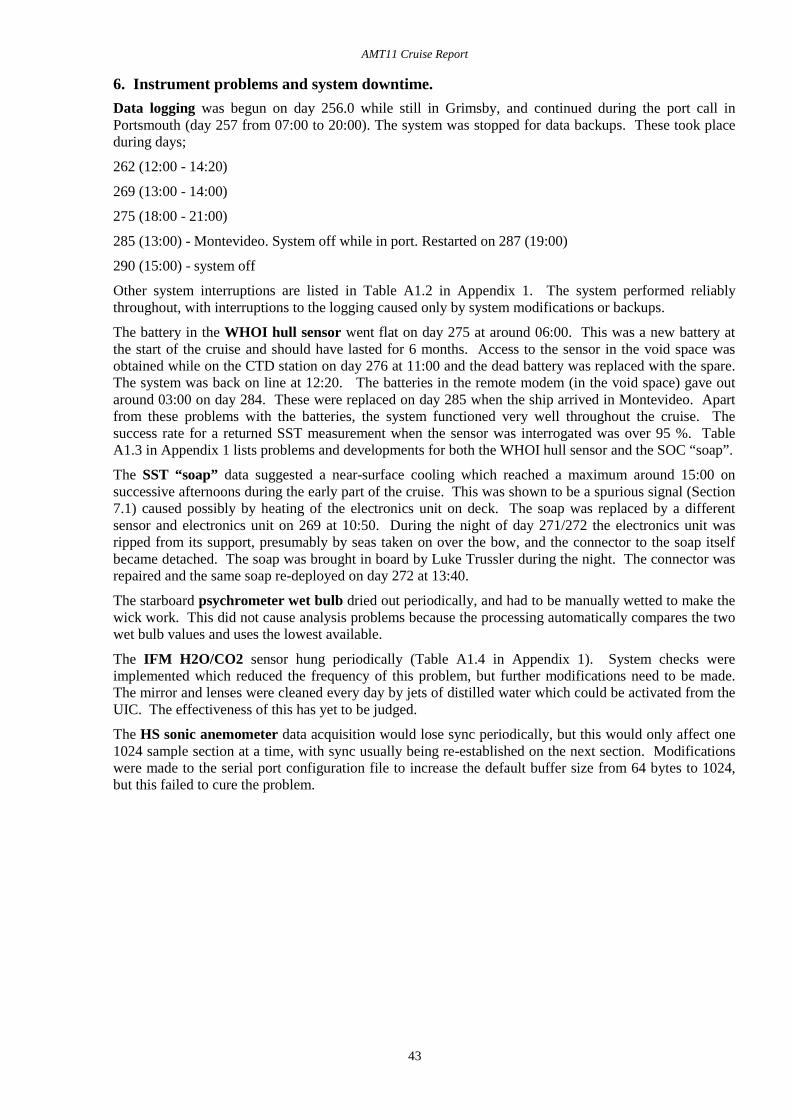
AMT11 Cruise Report

43

6. Instrument problems and system downtime. Data logging was begun on day 256.0 while still in Grimsby, and continued during the port call in Portsmouth (day 257 from 07:00 to 20:00). The system was stopped for data backups. These took place during days;

262 (12:00 - 14:20)

269 (13:00 - 14:00)

275 (18:00 - 21:00)

285 (13:00) - Montevideo. System off while in port. Restarted on 287 (19:00)

290 (15:00) - system off

Other system interruptions are listed in Table A1.2 in Appendix 1. The system performed reliably throughout, with interruptions to the logging caused only by system modifications or backups.

The battery in the WHOI hull sensor went flat on day 275 at around 06:00. This was a new battery at the start of the cruise and should have lasted for 6 months. Access to the sensor in the void space was obtained while on the CTD station on day 276 at 11:00 and the dead battery was replaced with the spare. The system was back on line at 12:20. The batteries in the remote modem (in the void space) gave out around 03:00 on day 284. These were replaced on day 285 when the ship arrived in Montevideo. Apart from these problems with the batteries, the system functioned very well throughout the cruise. The success rate for a returned SST measurement when the sensor was interrogated was over 95 %. Table A1.3 in Appendix 1 lists problems and developments for both the WHOI hull sensor and the SOC “soap”.

The SST “soap” data suggested a near-surface cooling which reached a maximum around 15:00 on successive afternoons during the early part of the cruise. This was shown to be a spurious signal (Section 7.1) caused possibly by heating of the electronics unit on deck. The soap was replaced by a different sensor and electronics unit on 269 at 10:50. During the night of day 271/272 the electronics unit was ripped from its support, presumably by seas taken on over the bow, and the connector to the soap itself became detached. The soap was brought in board by Luke Trussler during the night. The connector was repaired and the same soap re-deployed on day 272 at 13:40.

The starboard psychrometer wet bulb dried out periodically, and had to be manually wetted to make the wick work. This did not cause analysis problems because the processing automatically compares the two wet bulb values and uses the lowest available.

The IFM H2O/CO2 sensor hung periodically (Table A1.4 in Appendix 1). System checks were implemented which reduced the frequency of this problem, but further modifications need to be made. The mirror and lenses were cleaned every day by jets of distilled water which could be activated from the UIC. The effectiveness of this has yet to be judged.

The HS sonic anemometer data acquisition would lose sync periodically, but this would only affect one 1024 sample section at a time, with sync usually being re-established on the next section. Modifications were made to the serial port configuration file to increase the default buffer size from 64 bytes to 1024, but this failed to cure the problem.

AMT11 Cruise Report

44

7. Initial results.

7.1 Sea surface temperature measurements. There were four SST sensors in use; the CTD (various depths, accuracy of 0.001°), TSG (intake at 7 m, accuracy 0.01°), soap (surface, accuracy 0.1°) and WHOI sensor (depth of 3.5 m, accuracy unknown). From day 259 to 266, the soap was raised to the surface during the second CTD cast of the day (around 11:00 GMT), but for the first cast at around 05:00 the soap was not raised and would sink to a depth of 4 to 7 m. The CTD data from the first 10 casts were each averaged into ten 1m depth bins, from zero to 10 m. The files included data from both the up- and the down-casts. The depth bins spanned a time period of around 30 seconds, and this interval was used to average the 10 second values from the soap.

263262261260259258-0.2

-0.1

0.0

0.1

0.2

0.3

0.4

0.5

0.6

all depths0 to 1 m depth

3 to 7 m depth

Jday

soap

- ct

d te

mp1

Figure 3. Soap - CTD temp1 SST differences for the first nine CTD casts.

265264263262261260259258-0.5

-0.4

-0.3

-0.2

-0.1

0.0

0.1

0.2

0.3

Jday

tem

p1-te

mp2

Figure 4. Difference in the CTD sensor temperatures against Jday.

Figure 3 shows the difference between the soap and CTD (temp1 channel) temperatures from the various depths. The data is scattered by about 0.1°, but there is not enough data to show any significant offset. The large difference which occurred during day 259 was thought to be due to a problem with the CTD rather than the soap data. Figure 4 shows the difference between the SST data from the two temperature sensors on the CTD.

The two sensors usually agree to within 0.003° but there are periods when the difference reaches 0.5°. A -0.5° offset in the CTD temp sensor 1 would be consistent with the disparities seen in Figures 3 and 4.

AMT11 Cruise Report

45

This offset is confirmed by the comparison between the ship’s thermosalinograph (TSG) temperatures and that from the CTD temp1 sensor (Figure 5). However, the scatter which occurs in Figure 4 during days 262 and 263 does not occur in either the soap or TSG comparisons, which suggests that on these occasions the CTD temp2 sensor may be at fault. This is confirmed in Figure 6 which shows the difference between the TSG and the CTD temp2 sensor. Finally, replaying the CTD casts showed that on cast 3 (day 259) the temp1 channel on the upcast lagged behind the temp2 channel. It was concluded that on this occasion the pumped flow to the temp1 sensor may have become blocked. No further examination of the CTD casts were made during the cruise, but it is recommended that both channels should be examined for every cast to check for recurrences of the problem.

A direct comparison between the TSG and the soap is shown in Figure 6. It can be seen that the difference between the two varied with time of day. As the day progressed, the soap SST became increasingly colder compared to the TSG, reaching a maximum offset of -0.2° at around 15:00 GMT. This is the opposite trend which would occur if the water temperature at 7 m stays relatively constant, and the surface waters are heated up during the day. Also shown is a comparison of the soap SST with the WHOI SST for one day; the same trend is seen which confirms that it is due to the soap data rather than the TSG. The cool surface “skin effect” is only seen in the first few microns, and can not be the cause of the cooling seen by the soap at a depth of a few cm or more. It was thought that there may have been a problem due to heating of the soap electronics unit on deck. This will not be confirmed until post-cruise calibrations have been performed. However, the AMT PSO kindly agreed to perform an extra CTD dip during the afternoon of day 268 at about 15:00 which confirmed that the surface cooling effect was indeed spurious; repeated shallow surface profiles with the CTD proved that there was no surface cooled layer.

264263262261260259258-0.2

-0.1

0.0

0.1

0.2

0.3

0.4

0.5

Jday

tsg

- ctd

1 (3

to 7

m)

Figure 5. TSG - CTD temp1 SST differences between 3 and 7 m.

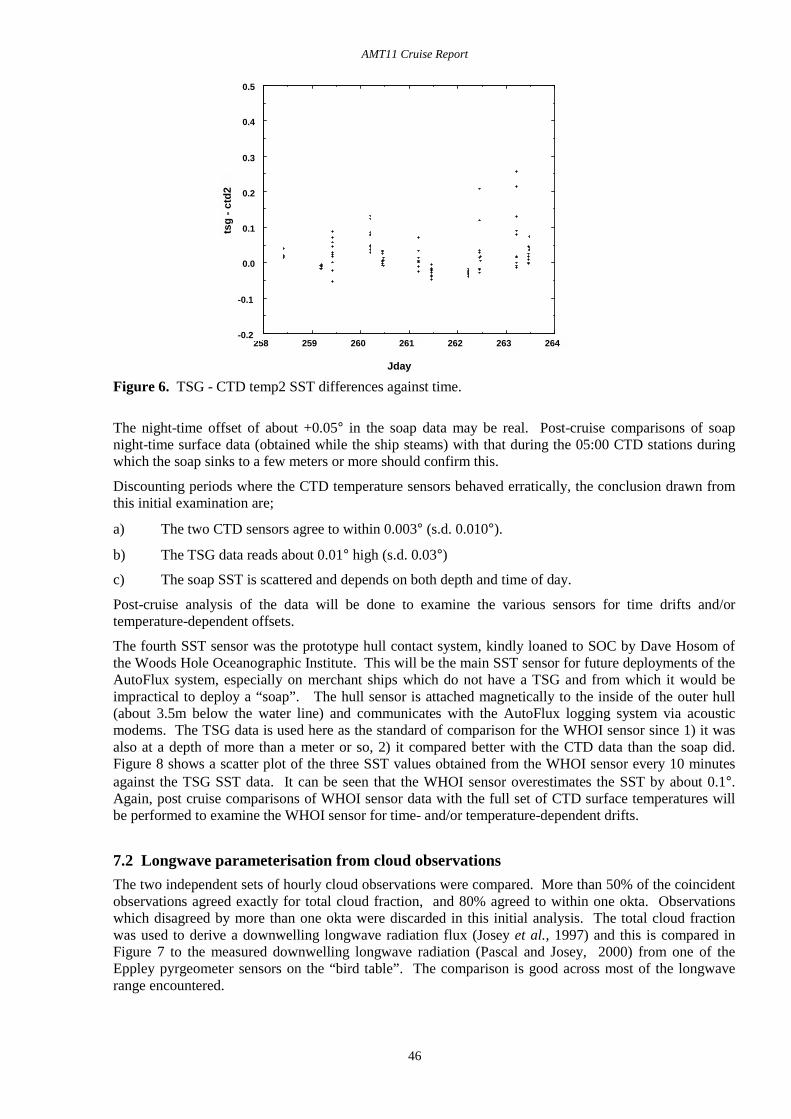
AMT11 Cruise Report

46

264263262261260259258-0.2

-0.1

0.0

0.1

0.2

0.3

0.4

0.5

Jday

tsg

- ctd

2

Figure 6. TSG - CTD temp2 SST differences against time. The night-time offset of about +0.05° in the soap data may be real. Post-cruise comparisons of soap night-time surface data (obtained while the ship steams) with that during the 05:00 CTD stations during which the soap sinks to a few meters or more should confirm this.

Discounting periods where the CTD temperature sensors behaved erratically, the conclusion drawn from this initial examination are;

a) The two CTD sensors agree to within 0.003° (s.d. 0.010°).

b) The TSG data reads about 0.01° high (s.d. 0.03°)

c) The soap SST is scattered and depends on both depth and time of day.

Post-cruise analysis of the data will be done to examine the various sensors for time drifts and/or temperature-dependent offsets.

The fourth SST sensor was the prototype hull contact system, kindly loaned to SOC by Dave Hosom of the Woods Hole Oceanographic Institute. This will be the main SST sensor for future deployments of the AutoFlux system, especially on merchant ships which do not have a TSG and from which it would be impractical to deploy a “soap”. The hull sensor is attached magnetically to the inside of the outer hull (about 3.5m below the water line) and communicates with the AutoFlux logging system via acoustic modems. The TSG data is used here as the standard of comparison for the WHOI sensor since 1) it was also at a depth of more than a meter or so, 2) it compared better with the CTD data than the soap did. Figure 8 shows a scatter plot of the three SST values obtained from the WHOI sensor every 10 minutes against the TSG SST data. It can be seen that the WHOI sensor overestimates the SST by about 0.1°. Again, post cruise comparisons of WHOI sensor data with the full set of CTD surface temperatures will be performed to examine the WHOI sensor for time- and/or temperature-dependent drifts.

7.2 Longwave parameterisation from cloud observations The two independent sets of hourly cloud observations were compared. More than 50% of the coincident observations agreed exactly for total cloud fraction, and 80% agreed to within one okta. Observations which disagreed by more than one okta were discarded in this initial analysis. The total cloud fraction was used to derive a downwelling longwave radiation flux (Josey et al., 1997) and this is compared in Figure 7 to the measured downwelling longwave radiation (Pascal and Josey, 2000) from one of the Eppley pyrgeometer sensors on the “bird table”. The comparison is good across most of the longwave range encountered.

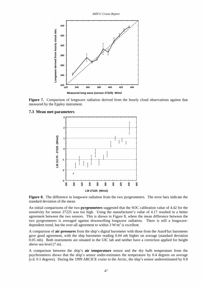
AMT11 Cruise Report

47

440420400380360340320320320

340

360

380

400

420

440

Measured long wave (sensor 27225) W/m2

Long

wav

e de

rived

from

hou

rly c

loud

obs

.

Figure 7. Comparison of longwave radiation derived from the hourly cloud observations against that measured by the Eppley instrument.

7.3 Mean met parameters

460

440

420

400

380

360

340

320

300

280

-3

-2

-1

0

1

2

3

LW 27225 (W/m2)

LW 3

1170

- 27

225

(W/m

2)

Figure 8. The difference in longwave radiation from the two pyrgeometers. The error bars indicate the standard deviation of the mean.

An initial comparisons of the two pyrgeometers suggested that the SOC calibration value of 4.42 for the sensitivity for sensor 27225 was too high. Using the manufacturer’s value of 4.17 resulted in a better agreement between the two sensors. This is shown in Figure 8, where the mean difference between the two pyrgeometers is averaged against downwelling longwave radiation. There is still a longwave-dependent trend, but the over-all agreement to within 3 W/m2 is excellent.

A comparison of air pressures from the ship’s digital barometer with those from the AutoFlux barometer gave good agreement, with the ship barometer reading 0.04 mb higher on average (standard deviation 0.05 mb). Both instruments are situated in the UIC lab and neither have a correction applied for height above sea level (7 m).

A comparison between the ship’s air temperature sensor and the dry bulb temperature from the psychrometers shows that the ship’s sensor under-estimates the temperature by 0.4 degrees on average (s.d. 0.1 degrees). During the 1999 ARCICE cruise to the Arctic, the ship’s sensor underestimated by 0.8

AMT11 Cruise Report

48

degrees (s.d. 0.2) which suggests a temperature-dependent calibration error on the ship’s sensor. The difference between the two psychrometer dry bulbs was 0.03 (s.d. 0.09).

Data from the ship’s anemometer were compared to that from the HS sonic anemometer. It was thought that the HS anemometer was not oriented exactly for-aft, and that it was pointed to port by about 5 degrees. This was confirmed by a comparison of relative wind direction from the two instruments, which suggested a 7 degree offset on the HS sonic relative wind direction for winds directly onto the bow, i.e. the relative wind directions from the HS overestimate by 7 degrees. A comparison of relative wind speeds show that the ship’s anemometer reads high by about 6% compared to the HS. The ship anemometer is mounted at a height of 20 m whereas the HS is at 16 m. This height difference would result in the ship anemometer reading high by 3 % (due to the logarithmic vertical profile of wind speed), i.e. it is thought that the ship anemometer has a calibration error of about 5% (the HS sonic was calibrated prior to the cruise).

7.4 Navigation systems A comparison of the ship’s heading from the gyro (true heading) data stream with that from the AutoFlux fluxgate compass (magnetic heading) showed reasonable agreement in the mean. Fifteen minute averaged data showed a scatter of 8 degrees (standard deviation). Ship speed over the ground from the nmea data stream and the AutoFlux GPS agreed very well on average (to within a few cm/s). However, there was one period when the two differed by up to 2 m/s. This is shown in Figure 11, which displays a time series of ship speed from the two systems from day 276 to day 279. It can be seen that the data from the AutoFlux navigation system is overestimating by up to 2 m/s during the latter part of day 277. This period coincided with the time that alterations were made to the sampling rate of the AutoFlux navigation system, but further investigation is needed to confirm the cause of the erroneous speeds.

8. Summary. By the fourth week of JR52 the system was automatically producing hourly direct measurements of the air-sea fluxes and was sending summary messages of the data back to SOC via the ORBCOMM satellite communications system in near real time.

Major system developments achieved during the cruise included;

• The ORBCOMM communication system was fully integrated into the AutoFlux system and automatically sent hour summary data back to SOC. The ORBCOMM management program “orby” performed reliably.

• The WHOI sea surface temperature system was installed successfully and was also fully integrated into the AutoFlux system using the program “acm”.

• The system time synchronisation program was merged into the GPS management program in order to free up a serial port which was required for the ORBCOMM system.

• A suite of nine UNIX scripts were written to process all the data streams, merge them together and calculate the surface fluxes. Execution of these scripts was managed by the program “scp”, which ran the UNIX scripts every hour.

Other system developments are listed in Table A1.1 in Appendix 1.

A new full-screen display was produced to plot the calculated surface fluxes as well as the mean meteorological parameters in near-real time (using data which are 30 to 60 minutes old). This is illustrated in Figure 12. The performance of the prototype IFM H2O/CO2 sensor and the sonic temperature sensor will be examined thoroughly post-cruise, as will the quality of the fluxes produced by these instruments.

Time series of the mean meteorological conditions and the calculated surface fluxes are displayed in the Figures in Appendix 2.

References AutoFlux group, 1996: AutoFlux - an autonomous system for monitoring air-sea fluxes using the inertial dissipation method and ship mounted instrumentation. Proposal to MAST research area C - Marine Technology, 38 pp. + appendices

AMT11 Cruise Report

49

Josey, S. A., D. Oakley and R. W. Pascal, 1997: On estimating the atmospheric longwave flux at the ocean surface from ship meteorological reports. J. Geophy. Res., 102 (C13), 27961 - 27972.

Pascal, R. W. and S. A. Josey, 2000: Accurate radiometric measurement of the atmospheric longwave flux at the sea surface. J. Atmos. Oceanic Technol., in press.

Pascal, R. W., M. J. Yelland and C. H. Clayson, 2000: The AutoFlux logging system - draft handbook. James Rennell Division, Southampton Oceanographic Centre, Southampton, U. K.

Smith, S. D., 1980: Wind Stress and Heat Flux over the Ocean in Gale Force Winds. J. Phys. Oceanogr., 10, 709-726.

Woodward, M, 2000: Atlantic Meridional Transect (AMT-11), September/October 2000, Cruise Report. Plymouth Marine Laboratory, U. K.

Yelland, M. J., B. I. Moat, P. K. Taylor, R. W. Pascal, J. Hutchings and V. C. Cornell, 1998: Wind stress measurements from the open ocean corrected for airflow disturbance by the ship. J. Phys. Oceanogr., 28, 1511 - 1526.

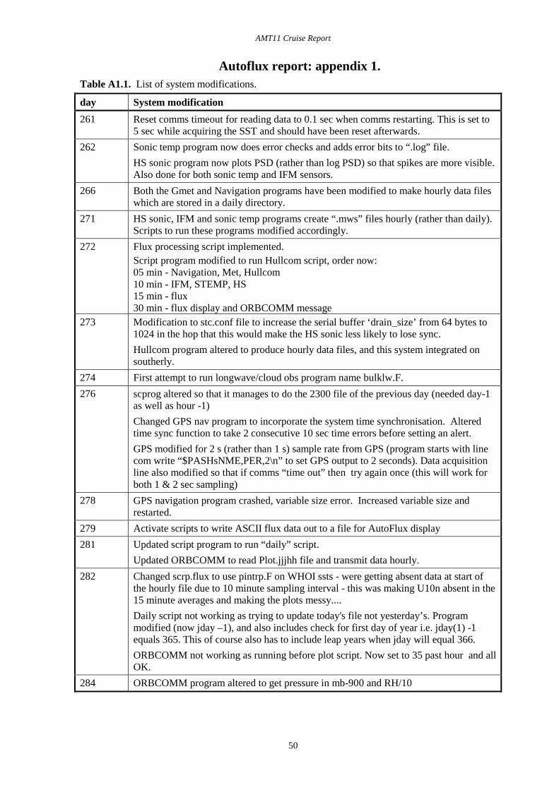
AMT11 Cruise Report

50

Autoflux report: appendix 1. Table A1.1. List of system modifications.

day System modification 261 Reset comms timeout for reading data to 0.1 sec when comms restarting. This is set to

5 sec while acquiring the SST and should have been reset afterwards. 262 Sonic temp program now does error checks and adds error bits to “.log” file.

HS sonic program now plots PSD (rather than log PSD) so that spikes are more visible. Also done for both sonic temp and IFM sensors.

266 Both the Gmet and Navigation programs have been modified to make hourly data files which are stored in a daily directory.

271 HS sonic, IFM and sonic temp programs create “.mws” files hourly (rather than daily). Scripts to run these programs modified accordingly.

272 Flux processing script implemented. Script program modified to run Hullcom script, order now: 05 min - Navigation, Met, Hullcom 10 min - IFM, STEMP, HS 15 min - flux 30 min - flux display and ORBCOMM message

273 Modification to stc.conf file to increase the serial buffer ‘drain_size’ from 64 bytes to 1024 in the hop that this would make the HS sonic less likely to lose sync. Hullcom program altered to produce hourly data files, and this system integrated on southerly.

274 First attempt to run longwave/cloud obs program name bulklw.F. 276 scprog altered so that it manages to do the 2300 file of the previous day (needed day-1

as well as hour -1) Changed GPS nav program to incorporate the system time synchronisation. Altered time sync function to take 2 consecutive 10 sec time errors before setting an alert. GPS modified for 2 s (rather than 1 s) sample rate from GPS (program starts with line com write “$PASHsNME,PER,2\n” to set GPS output to 2 seconds). Data acquisition line also modified so that if comms “time out” then try again once (this will work for both 1 & 2 sec sampling)

278 GPS navigation program crashed, variable size error. Increased variable size and restarted.

279 Activate scripts to write ASCII flux data out to a file for AutoFlux display 281 Updated script program to run “daily” script.

Updated ORBCOMM to read Plot.jjjhh file and transmit data hourly. 282 Changed scrp.flux to use pintrp.F on WHOI ssts - were getting absent data at start of

the hourly file due to 10 minute sampling interval - this was making U10n absent in the 15 minute averages and making the plots messy.... Daily script not working as trying to update today's file not yesterday’s. Program modified (now jday –1), and also includes check for first day of year i.e. jday(1) -1 equals 365. This of course also has to include leap years when jday will equal 366. ORBCOMM not working as running before plot script. Now set to 35 past hour and all OK.

284 ORBCOMM program altered to get pressure in mb-900 and RH/10

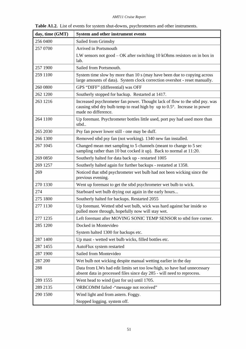
AMT11 Cruise Report

51

Table A1.2. List of events for system shut-downs, psychrometers and other instruments.

day, time (GMT) System and other instrument events 256 0400 Sailed from Grimsby 257 0700 Arrived in Portsmouth

LW sensors not good – OK after switching 10 kOhms resistors on in box in lab.

257 1900 Sailed from Portsmouth. 259 1100 System time slow by more than 10 s (may have been due to copying across

large amounts of data). System clock correction overshot - reset manually. 260 0800 GPS “DIFF” (differential) was OFF 262 1200 Southerly stopped for backup. Restarted at 1417. 263 1216 Increased psychrometer fan power. Thought lack of flow to the stbd psy. was

causing stbd dry bulb temp to read high by up to 0.5°. Increase in power made no difference.

264 1100 Up foremast. Psychrometer bottles little used, port psy had used more than stbd..

265 2030 Psy fan power lower still - one may be duff. 266 1300 Removed stbd psy fan (not working). 1340 new fan installed. 267 1045 Changed mean met sampling to 5 channels (meant to change to 5 sec

sampling rather than 10 but cocked it up). Back to normal at 11:20. 269 0850 Southerly halted for data back up - restarted 1005 269 1257 Southerly halted again for further backups - restarted at 1358. 269 Noticed that stbd psychrometer wet bulb had not been wicking since the

previous evening. 270 1330 Went up foremast to get the stbd psychrometer wet bulb to wick. 274 Starboard wet bulb drying out again in the early hours... 275 1800 Southerly halted for backups. Restarted 2055 277 1130 Up foremast. Wetted stbd wet bulb, wick was hard against bar inside so

pulled more through, hopefully now will stay wet. 277 1235 Left foremast after MOVING SONIC TEMP SENSOR to stbd fore corner. 285 1200 Docked in Montevideo

System halted 1300 for backups etc. 287 1400 Up mast - wetted wet bulb wicks, filled bottles etc. 287 1455 AutoFlux system restarted 287 1900 Sailed from Montevideo 287 200 Wet bulb not wicking despite manual wetting earlier in the day 288 Data from LWs had edit limits set too low/high, so have had unnecessary

absent data in processed files since day 285 - will need to reprocess. 289 1555 Went head to wind (just for us) until 1705. 289 2135 ORBCOMM failed -“message not received” 290 1500 Wind light and from astern. Foggy.

Stopped logging. system off.

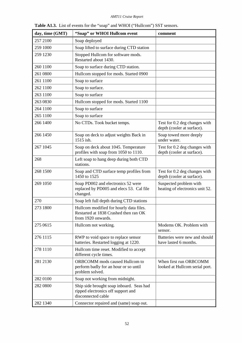
AMT11 Cruise Report

52

Table A1.3. List of events for the “soap” and WHOI (“Hullcom”) SST sensors.

day, time (GMT) “Soap” or WHOI Hullcom event comment 257 2100 Soap deployed 259 1000 Soap lifted to surface during CTD station 259 1230 Stopped Hullcom for software mods.

Restarted about 1430.

260 1100 Soap to surface during CTD station. 261 0800 Hullcom stopped for mods. Started 0900 261 1100 Soap to surface 262 1100 Soap to surface. 263 1100 Soap to surface 263 0830 Hullcom stopped for mods. Started 1100 264 1100 Soap to surface 265 1100 Soap to surface 266 1400 No CTDs. Took bucket temps. Test for 0.2 deg changes with

depth (cooler at surface). 266 1450 Soap on deck to adjust weights Back in

1515 ish. Soap towed more deeply under water.

267 1045 Soap on deck about 1045. Temperature profiles with soap from 1050 to 1110.

Test for 0.2 deg changes with depth (cooler at surface).

268 Left soap to hang deep during both CTD stations.

268 1500 Soap and CTD surface temp profiles from 1450 to 1525

Test for 0.2 deg changes with depth (cooler at surface).

269 1050 Soap PD002 and electronics 52 were replaced by PD005 and elecs 53. Cal file changed.

Suspected problem with heating of electronics unit 52.

270 Soap left full depth during CTD stations 273 1800 Hullcom modified for hourly data files.

Restarted at 1838 Crashed then ran OK from 1920 onwards.

275 0615 Hullcom not working. Modems OK. Problem with sensor.

276 1115 RWP to void space to replace sensor batteries. Restarted logging at 1220.

Batteries were new and should have lasted 6 months.

278 1110 Hullcom time reset. Modified to accept different cycle times.

281 2130 ORBCOMM mods caused Hullcom to perform badly for an hour or so until problem solved.

When first run ORBCOMM looked at Hullcom serial port.

282 0100 Soap not working from midnight. 282 0800 Ship side brought soap inboard. Seas had

ripped electronics off support and disconnected cable

282 1340 Connector repaired and (same) soap out.

AMT11 Cruise Report

53

Table A1.3 (continued). List of events for the “soap” and WHOI (“Hullcom”) SST sensors.

day, time (GMT) “Soap” or WHOI Hullcom event comment 284 0250 Hullcom remote modem batteries dying. 284 2205 Soap brought inboard ready for arrival in

Montevideo.

285 1600 Hullcom remote modem batteries replaced in Montevideo.

287 1800 Hullcom set to 10 minutes 287 1940 Soap deployed (sailed 1900) 287 2020 Hullcom program altered: flushes serial

port when first activates read data.

288 Hullcom data had edit limits set too low/high since day 285.

- will need to reprocess data.

AMT11 Cruise Report

54

Table A1.4. List of events for the IFM H2O/CO2 sensor.

day, time (GMT) IFM H2O/CO2 event comment 259 1154 washed lenses and mirror. 260 0906 washed lenses and mirror. 260 1500 260 1600

IFM failed to start at 1500 and again at 1600.

Program didn’t crash, but seemed to fail to complete processing in time for 1500 - don’t know why it didn’t start at 1600.

260 1615 Program restarted. 261 0942 washed 262 0907 washed 263 0600 Program hung. 263 0820 Program halted, data stream checked

with xterm / tip then restarted.

Had completed the processing of the data run started at 0500 but failed to restart the data stream for the next period at 0600.

263 1038 washed 263 1330 to 1345 washed MANUALLY 264 1100 ish washed MANUALLY

reservoir had lots of water, should squirt for longer

265 1237 washed for 20 sec 266 1230-1300 washed MANUALLY 266 1700 Hung at start of data acquisition at

1700, Quit program, start data with xterm, started program 1750

267 1126 washed 268 1045 washed 269 0955 washed 270 0941 washed 270 1340 washed MANUALLY 271 0800 Failed to start at 0800 - Quit program, start data with xterm,

started program 1750 271 1255 New version of program for hourly

“.mws” files launched. Mws files had previously been daily.

272 1951 washed 273 1053 washed 274 1156 washed 275 1100 Hung at start of acquisition. Quit prog, used tip to verify data

stream ok, then restarted prog. 275 1200 Hung at 1200. (OK at 1300) 275 1107 washed 276 1259 washed 277 1130 washed MANUALLY 277 1235 SENSOR MOVED FURTHER TO

PORT See Figure 2b

278 1335 washed

AMT11 Cruise Report

55

Table A1.4 (continued). List of events for the IFM H2O/CO2 sensor.

day, time (GMT) IFM H2O/CO2 event comment 278 2100 Missed 2100 start time. Left it to see

if it would catch the next hour - it did indeed.

due to measured humidity of ~300 g/m3? – may have had difficulty processing

280 1253 washed MANUALLY and braced sensor with string

281 2207 washed water reached the lenses or at least interrupted the path - head wind with relative speed of 18 m/s

282 1058 washed 283 1806 washed 284 0000 284 0300

0245 – saw that program had hung at 0000 trying to acquire data. Hung while “acquiring data” at 0300.

Quit program, ran xterm checked data stream ok then restarted.

284 1211 washed 287 1400 washed MANUALLY prior to

leaving Montevideo IFM comms problem sorted when southerly re-booted.

287 1956 washed 288 1159 washed 288 1500 Noticed that H2O values OK on

acquisition display, but become garbage when written to the “mws” data file. Problem caused by dimension of binary variable. Program modified and restarted at 1500.

Problem began on day 285 about 1130. Caused when the binary H2O data cast from double to short which has a maximum of 32768 which was exceeded by the reference value. Raw data OK and will be replayed post-cruise

288 1800 Noticed processed CO2 values low by about 50% compared to the real time display. The processed data had a different temp (20°) for the temp compensation value (display value 25°).

Will replay data with new software to use last hours air temp.

289 1521 washed? no evidence on display that water was reaching path

289 1548 washed? no evidence on display that water was reaching path

AMT11 Cruise Report

56

Marine Geophysics

Alex Cunningham & Neil Mitchell British Antarctic Survey/Oxford and Cardiff Universities

In addition to the AMT–11 core science programme, marine geophysical data were collected by scientists from the BAS Geological Sciences Division and Cardiff University (RRS James Clark Ross cruise JR53). This section provides a brief description of our activities and achievements. A more detailed account is included in the BAS JR53 Cruise Report. During JR53, we had two main objectives:

(1) To collect marine geophysical data opportunistically on passage between AMT–11 stations. This work constitutes the start of a proposed long-term project to collect data on passage to and from the Antarctic. Existing studies suggest that data collected on transit by RRS James Clark Ross could provide new insights into diverse topics such as plate motion history, mid-ocean ridge processes, continental margin processes, volcanic island morphology, slope stability and failure, and deep-sea sediment transport.

(2) To survey a short section of the Mid-Atlantic Ridge near 1o30’S. Marine geophysical data collected in this region would provide insights into the structure, morphology and tectonic evolution of spreading ridge segments south of the Chain Fracture Zone.

In order to meet these objectives, swath bathymetry and side-scan sonar data were collected using the Simrad EM 120 multibeam sonar which was installed on RRS James Clark Ross earlier in the year. The recorded EM 120 signal is used to form an array of 191 1o by 1o beams, making it one of the highest resolution hull-mounted deep water sonars available to academic researchers. Multibeam soundings were depth converted using sea water velocity–depth profiles obtained from XBTs or from the Applied Microsystems velocity profiler installed on the ship. In addition, we collected high-resolution acoustic reflection profiles using the Simrad TOPAS sub-bottom profiler, and magnetic data using shipboard three-component magnetometers.

Scientific Highlights Upon leaving the UK, our first scientific target was the continental margin in the Southwest Approaches, where we imaged canyons at the base of the continental slope. Here, the multibeam sonar provided some exciting new data on shelf edge canyons, showing three orders of geomorphological slope incision. Following some sedimentary structures within the Bay of Biscay, we recorded abyssal hills west of Iberia before crossing the Gloria Fault, the plate boundary between Europe and Africa.

To the west of the Canary Islands and Africa, we crossed some channels shown by previous IOS work to be caused by turbidity currents transporting sediments from the African margin, and subtle topography of the Canary and Saharan debris flows. Following a period without recording within the Cape Verdes 200 nmi EEZ, we resumed recording and collected multibeam data over some further turbidity current channels south of the islands, shown by Gebco charts to be sourced on the African margin. From there to the ridge area, we crossed a mostly featureless area, although a number of seamounts were identified on the Sierra Leone Rise.

Within the Mid-Atlantic Ridge area proper, we first crossed the inactive section of the Romanche Transform and the active Chain Transform, before beginning our box-shaped survey. The multibeam data (Fig. 1) cover both sides of an axial rift valley and inside corner high (a shallow region at the intersection of a rift valley with a short-offset transform to another rift valley). In contrast to many inside corner highs in the North Atlantic, this one does not show a surface with crenulations oriented parallel to spreading, which are evidence for large-offset detachment faulting, but rather it seems to have a similar fabric to ‘normal’ sea floor. Upon leaving the box survey, we ran single lines further down the ridge, covering some parts of other sections of rift valley floor and inside-corner highs, again showing no evidence of crenulations.

Upon leaving the survey area, we made one opportunistic line across the SW flank of Ascension Island, crossing a satellite volcano to the main Ascension Island edifice, while still remaining more than 12 nmi beyond the coastline as required by the MOD. Further west in the Brazil Basin, we covered mostly abyssal hill terrain, although seamounts and migrating sediment waves were imaged occasionally in this area.

AMT11 Cruise Report

57

Figure 1. Multibeam bathymetry of the Mid-Atlantic Ridge near 1o30’S.

AMT11 Cruise Report

58

Appendix 1: Noon Positions AMT-11, Sept/Oct 2000

DATE LAT LONG AVER SPEED

DISTANCE

WIND SEA

12/9/00 520 59.7’N 01028.2’E 10.58 WNW 3 Slight 13/9/00 POMPEY 14/9/00 490 34.47’N 05039.1’W 12.38 196 SW 3 Slight 15/9/00 470 02’N 11040.1’W 12.21 293 N 4 Moderate 16/9/00 420 53.4’N 14048.5’W 11.4 285 E 4 Moderate 17/9/00 380 50.7’N 17046.5’W 11.63 279 NxE 5 Moderate 18/9/00 340 48.4’N 20030.3’W 12.37 277 N 4 Moderate 19/9/00 300 25.0’N 21025.0’W 11.95 268 N 4 Moderate 20/9/00 26006.2’N 21045.9’W 11.69 263 NxE 4 Slight 21/9/00 21050.2’N 20059.1’W 11.74 261 ENE 4 Moderate 22/9/00 17018.7’N 20039.9’W 11.58 274 NE 4/5 Moderate 23/9/00 12037.6’N 20039.7’W 12.18 282 NxE 3 Slight 24/9/00 8042.8’N 18055.3’W 11.77 263 SW 3 Slight 25/9/00 5000.3’N 16052.8’W 11.74 256 SxW 4 Moderate 26/9/00 1015.3’N 14050.9’W 11.56 258 SSE 3/4 Slight 27/9/00 1051.9’S 13008.0’W 11.65 256 SSE 3 Slight 28/9/00 1042.6’S 12043.0’W 11.75 263 SxE 3 Slight 29/9/00 4032.7’S 12043.1’W 11.59 268 SxE 4 Slight 30/9/00 8005.8’S 14055.6’W 11.38 254 SE 3/4 Slight 1/10/00 10058.4’S 18020.3’W 11.45 266 SSE 3 Slight 2/10/00 13043.7’S 21039.2’W 11.52 256 SE 4/5 Moderate 3/10/00 16027.2’S 24056.9’W 11.47 252 ExS 5 Moderate 4/10/00 19011.6’S 28019.3’W 11.42 254 N 3/4 Slight 5/10/00 21049.2’S 31036.4’W 11.59 244 NW 3 Slight 6/10/00 24037.4’S 35009.8’W 11.19 261 NW 4 Slight/Mod. 7/10/00 27021.9’S 38045.9’W 11.55 255 WxS 6 Rough. 8/10/00 30006.8’S 42024.2’W 11.55 253 SW 5 Mod/Rough 9/10/00 33012.8’S 46042.0’W 12.93 288 NE 5 Rough 8/10/00 35005.8’S 52011.5’W 12.52 313 SWxW 5 Rough

AMT11 Cruise Report

59

Appendix 2: AMT-11, Salinity Bottles, Analysed on the AUTOSAL, 8/10/00

Standard Seawater, IAPSO. Batch p137, 09-dec-99 K15=0.99995, Salinity=34.998 Colour Number Value 1 Value 2 Value 3 Value 4 Blue 5:18 2.0354 2.03548 2.0355 2.0355 Blue S:16 2.04365 2.04365 Blue S:3 2.0563 2.05628 Blue S:4 2.07374 Blue S:5 2.09624 Blue S:8 2.08075 2.08069 2.08075 Blue S:7 2.08837 2.08833 2.08826 Blue S:6 2.10036 2.13306 Blue S:17 2.08132 20.8132 Blue S:14 2.09863 2.09862 Blue S:13 2.075 2.04749 Blue S:2 2.07246 2.07232 2.07235 Blue S:10 2.0186 2.0186 Blue S:11 2.04777 2.04776 Blue S:12 2.05743 2.05742 Blue S:23 1.97852 1.97849 1.97846 Blue S:1 2.00651 2.00648 Blue S:19 2.01235 2.01233 Blue S-15 2.04628 2.04626 Blue S-20 2.00084 2.0084 Blue S:21 2.02701 2.02693 2.02692 Blue S:22 2.01149 2.01145 Blue S:9 2.01551 2.01544 2.01538 Blue S:24 2.03079 2.03082 Red 02:02 2.04892 2.04901 2.04903 02:01 2.00086 2.00086 02:04 2.04178 2.04174 02:05 2.04174 2.04176 02:07 2.04531 2.04531 02:10 2.01468 2.01468 02:08 2.09648 2.09647 02:09 2.09504 2.09498 02:12 2.02998 2.02998 02:11 2.11153 2.11131 2.11127 2.1114 2.11139 02:13 2.06477 2.06477 02:14 2.04535 2.04534 02:15 2.02123 2.02123 02:16 2.02579 2.02579 2.02579 02:17 2.05536 2.05536

AMT11 Cruise Report

60

Appendix 3: XBT deployment log

DATE GMT LAT LON SST Salinity Probe Filename 14/9/00 1126 49o32.78'N 5o47.74'W 17.2 35.27 T7 T7_01029 14/9/00 1700 49o03.17'N 7o22.25'W 18.0 35.25 T7 T7_01030 15/9/00 0520 47o55.22'N 10o44.78'W 18.7 35.62 T7 T7_01034 15/9/00 1119 46o59.21'N 11o42.45'W 19.4 35.66 T5 T5_01035 15/9/00 1632 46o01.99'N 12o12.55'W 19.9 35.71 T5 T5_01036 15/9/00 2158 45o17.15'N 13o02.18'W 20.0 35.64 T7 T7_01037 15/9/00 2204 45o17.15'N 13o02.18'W 20.1 35.64 T7 T7_01038 16/9/00 1123 42o58.22'N 14o45.02'W 21.3 35.79 T5 T5_01039 16/9/00 1206 42o52.38'N 14o49.33'W 21.4 35.77 T7 T7_01040 16/9/00 1909 41o38.31'N 15o46.02'W 21.5 35.85 T7 T7_01041 16/9/00 2340 41o07.39'N 16o08.88'W 21.1 35.95 T7 T7_01042 17/9/00 0530 39o54.45'N 17o01.07'W 21.4 36.21 T7 T7_01043 17/9/00 1122 38o57.49'N 17o42.02'W 21.6 36.42 T5 T5_01044 17/9/00 2345 36o45.53'N 19o12.88'W 22.2 36.32 T7 T7_01045 18/9/00 0638 35o38.79'N 19o57.66'W 22.6 36.47 T7 T7_01046 18/9/00 1112 34o55.81'N 20o27.56'W 23.5 36.85 T5 T5_01047 18/9/00 2340 33o48.99'N 20o43.26'W 24.1 36.84 T7 T7_01049 19/9/00 0600 31o27.53'N 21o12.80'W 23.9 36.95 T7 T7_01050 19/9/00 1121 30o32.43'N 21o23.60'W 24.0 36.93 T5 T5_01051 19/9/00 1718 29o24.48'N 21o37.03'W 24.2 37.15 T7 T7_01052 19/9/00 2344 28o20.82'N 21o49.30'W 23.9 37.01 T7 T7_01053 20/9/00 0613 27o04.10'N 21o56.21'W 23.9 37.16 T7 T7_01055 20/9/00 1117 26o13.09'N 21o47.18'W 23.9 37.16 T5 T5_01056 20/9/00 2340 24o22.95'N 21o26.65'W 24.3 36.64 T7 T7_01058 21/9/00 0604 22o50.44'N 21o10.20'W 24.0 36.36 T7 T7_01059 21/9/00 1127 21o56.52'N 21o00.11'W 24.5 36.24 T5 T5_01061 21/9/00 1622 21o03.71'N 20o51.26'W 24.8 36.28 T5 T5_01064 21/9/00 1956 20o23.97'N 20o44.43'W 24.7 36.23 T5 T5_01066 21/9/00 2342 18o22.23'N 20o36.32'W 25.2 36.24 T5 T5_01067 23/9/00 1122 12o44.47'N 20o39.90'W 28.5 36.07 T5 T5_01068 23/9/00 1715 11o38.84'N 20o33.79'W 28.5 35.52 T7 T7_01069 23/9/00 2345 10o32.40'N 19o56.29'W 28.4 34.93 T7 T7_01070 24/9/00 0809 09o14.61'N 19o13.66'W 27.5 34.07 T7 T7_01071 24/9/00 1120 08o49.00'N 18o58.46'W 27.5 34.36 T5 T5_01072 24/9/00 1732 07o52.92'N 18o28.48'W 27.8 34.58 T7 T7_01073 24/9/00 2342 06o59.18'N 17o59.64'W 27.7 34.26 T7 T7_01074 25/9/00 1122 05o06.06'N 16o55.86'W 27.3 34.95 T5 T5_01075 25/9/00 1741 04o01.59'N 16o21.46'W 27.2 35.53 T7 T7_01076 25/9/00 2353 02o58.22'N 15o47.11'W 26.2 35.55 T7 T7_01077 26/9/00 0602 02o06.00'N 15o19.03'W 24.3 35.56 T7 T7_01078 26/9/00 1122 01o21.15'N 14o52.81'W 23.6 35.81 T5 T5_01079 26/9/00 1754 00o16.17'N 14o18.55'W 23.5 36.00 T7 T7_01080 27/9/00 0529 01o23.65'S 13o12.03'W 23.2 35.87 T7 T7_01081 27/9/00 1036 02o07.24'S 13o08.38'W 23.5 35.89 T5 T5_01082 27/9/00 1735 01o50.87'S 13o02.99'W 23.5 35.87 T7 T7_01083 27/9/00 2350 01o25.20'S 12o55.98'W 23.3 35.87 T7 T7_01084 28/9/00 0504 02o08.55'S 12o48.83'W 23.4 35.82 T7 T7_01085

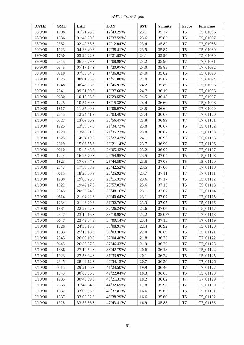
AMT11 Cruise Report

61

DATE GMT LAT LON SST Salinity Probe Filename 28/9/00 1008 01o21.78'S 12o43.29'W 23.1 35.77 T5 T5_01086 28/9/00 1736 01o45.00'S 12o37.59'W 23.6 35.85 T5 T5_01087 28/9/00 2352 02o40.63'S 12o12.04'W 23.4 35.82 T7 T7_01088 29/9/00 1123 04o38.40'S 12o38.41'W 23.9 35.87 T5 T5_01089 29/9/00 1730 05o20.22'S 13o21.85'W 24.1 35.96 T5 T5_01090 29/9/00 2345 06o55.79'S 14o08.98'W 24.2 35.90 T7 T7_01091 30/9/00 0545 07o17.17'S 14o20.07'W 24.0 35.85 T7 T7_01092 30/9/00 0910 07o50.04'S 14o36.82'W 24.0 35.82 T5 T5_01093 30/9/00 1125 08o01.75'S 14o51.08'W 24.0 35.82 T5 T5_01094 30/9/00 1748 08o48.33'S 15o45.91'W 24.2 35.89 T5 T5_01095 30/9/00 2341 09o31.90'S 16o37.60'W 24.7 36.19 T7 T7_01096 1/10/00 0630 10o15.86'S 17o29.55'W 24.5 36.43 T7 T7_01097 1/10/00 1225 10o54.30'S 18o15.38'W 24.4 36.60 T5 T5_01098 1/10/00 1817 11o37.40'S 19o06.97'W 24.5 36.64 T7 T7_01099 1/10/00 2345 12o24.41'S 20o03.40'W 24.4 36.67 T7 T7_01100 2/10/00 0727 13o09.20'S 20o56.47'W 23.8 36.99 T7 T7_01101 2/10/00 1225 13o39.87'S 21o34.72'W 23.8 36.87 T5 T5_01102 2/10/00 1229 13o40.31'S 21o35.22'W 23.8 36.87 T5 T5_01103 2/10/00 1825 14o24.10'S 22o27.42'W 24.1 36.95 T5 T5_01105 2/10/00 2319 15o08.55'S 23o21.14'W 23.7 36.99 T7 T7_01106 3/10/00 0610 15o45.43'S 24o05.42'W 23.2 36.97 T7 T7_01107 3/10/00 1244 16o25.70'S 24o54.95'W 23.5 37.04 T5 T5_01108 3/10/00 1823 17o06.47'S 25o44.59'W 23.5 37.08 T5 T5_01109 3/10/00 2347 17o53.38'S 26o42.52'W 23.5 37.06 T7 T7_01110 4/10/00 0615 18o28.00'S 27o25.92'W 23.7 37.11 T7 T7_01111 4/10/00 1230 19o08.23'S 28o15.31'W 23.6 37.17 T5 T5_01112 4/10/00 1822 19o42.17'S 28o57.82'W 23.6 37.13 T5 T5_01113 4/10/00 2345 20o29.24'S 29o48.16'W 23.1 37.07 T7 T7_01114 5/10/00 0614 21o04.22'S 30o40.64'W 23.1 37.07 T7 T7_01115 5/10/00 1234 21o46.29'S 31o32.76'W 23.3 37.05 T5 T5_01116 5/10/00 1831 22o29.02'S 32o26.24'W 23.6 37.06 T5 T5_01117 5/10/00 2347 23o10.16'S 33o18.98'W 23.2 35.08? T7 T7_01118 6/10/00 0647 23o49.34'S 34o09.14'W 23.4 37.13 T7 T7_01119 6/10/00 1328 24o36.13'S 35o08.91'W 22.4 36.92 T5 T5_01120 6/10/00 1933 25o18.18'S 36o03.36'W 22.0 36.69 T5 T5_01121 6/10/00 2345 26o05.10'S 37o04.40'W 21.8 36.73 T7 T7_01122 7/10/00 0645 26o37.57'S 37o46.43'W 21.9 36.76 T7 T7_01123 7/10/00 1336 27o19.62'S 38o42.79'W 20.6 36.18 T5 T5_01124 7/10/00 1923 27o58.94'S 31o33.97'W 20.1 36.24 T5 T5_01125 7/10/00 2345 28o44.12'S 40o34.15'W 20.7 36.50 T7 T7_01126 8/10/00 0515 29o21.56'S 41o24.50'W 19.9 36.46 T7 T7_01127 8/10/00 1343 30o05.36'S 42o22.04'W 18.3 36.03 T5 T5_01128 8/10/00 1935 30o48.09'S 43o21.31'W 18.2 36.02 T7 T7_01129 8/10/00 2355 31o40.64'S 44o32.69'W 17.8 35.96 T7 T7_01130 9/10/00 1332 33o09.55'S 46o37.81'W 16.6 35.63 T5 T5_01131 9/10/00 1337 33o09.92'S 46o38.29'W 16.6 35.60 T5 T5_01132 9/10/00 1928 33o57.36'S 47o43.41'W 16.9 35.83 T7 T7_01133

AMT11 Cruise Report

62

Appendix 4. Underway night watch, sampling and observation Time Fluorescence Date

Local GMT Latitude Longitude Temperature Salinity

O/L TIF Sample No. Chl

Volume filtered Chl (ml)

[Chla] µg/l

14/09/00 0806 0706 49°47.79’N 04°37.49’W 17.10 35.07 20.9 2.2 001 200 51.3 14/09/00 1328 1228 49°27.43’N 06°08.81’W 17.46 35.36 10.7 1.1 002 200 12.6 14/09/00 1628 1528 49°10.96’N 07°00.84’W 18.10 35.21 7.5 0.8 003 200 5.95 14/09/00 2006 1906 48°50.47’N 07°59.51’W 17.89 35.42 6.6 0.6 004 200 2.92 15/09/00 0001 2301 48°26.89’N 09°08.58’W 17.70 35.52 9.3 1.0 005 200 3.47 15/09/00 0802 0702 47°39.33’N 11°08.89’W 18.70 35.63 6.3 2.3 006 200 3.74 15/09/00 1334 1234 46°44.97’N 11°52.51'W 19.54 35.68 52.7 5.2 007 200 2.41 15/09/00 1554 1454 46°19.46'N 12°12.58'W 19.91 35.72 51.0 5.2 008 200 2.28 15/09/00 2019 1919 45°32.12'N 12°50.72'W 19.09 35.68 53.1 5.4 009 200 2.92 15/09/00 2315 2215 45°17.67'N 13°02.18'W 15.25 35.63 56.4 1.8 010 200 3.32 16/09/00 0803 0803 42°07.29'N 14°28.70'W 21.00 35.71 53.4 1.7 011 200 2.45 16/09/00 1405 1405 47°32.46'N 15°06.15'W 21.80 35.79 47.0 1.5 012 200 1.56 16/09/00 1614 1614 42°10.05'N 15°23.89'W 21.90 35.88 46.1 1.5 013 200 1.84 16/09/00 2006 2006 41°27.56'N 15°53.96'W 21.40 35.94 55.0 1.8 014 200 1.79 16/09/00 2355 2355 41°07.39'N 16°08.88'W 21.20 35.90 50.0 1.6 015 200 1.94 17/09/00 0822 0822 39°23.99'N 17°23.42'W 21.50 36.21 49.3 1.55 016 200 2.44 17/09/00 1344 1344 38°31.36'N 18°00.83'W 21.70 36.39 46.7 1.5 017 200 1.93 17/09/00 1700 1700 37°56.73'N 18°24.19'W 22.00 36.45 45.7 1.5 018 200 17/09/00 2043 2043 37°17.66'N 18°50.54'W 21.90 36.29 45.5 1.5 019 200 1.47 17/09/00 2352 2352 37°21.17'N 18°48.06'W 22.10 36.30 45.4 1.5 020 200 1.41 18/09/00 0801 0801 35°23.29'N 20°07.64'W 23.20 36.56 44.7 1.4 021 200 1.61 18/09/00 1321 1321 34°32.43'N 20°34.27'W 23.40 36.73 43.0 022 200 1.37 18/09/00 1658 1658 33°49.12'N 20°43.29'W 23.50 36.71 44.2 1.4 023 200 1.23 18/09/00 2001 2001 33°12.55'N 20°50.82'W 23.70 36.70 43.4 1.4 024 200 1.10 18/09/00 2350 2350 33°49.99'N 20°43.26'W 24.10 36.80 44.1 1.4 025 200 0.99 19/09/00 0755 0755 31°04.03'N 21°16.82'W 23.90 36.94 43.3 1.4 026 250 1.32 19/09/00 1345 1345 30°04.80'N 21°28.74'W 24.35 37.18 41.5 1.4 027 250 1.07 19/09/00 1650 1650 29°29.83'N 21°35.91'W 24.24 37.26 42.0 1.4 028 250 0.92 19/09/00 2011 2011 28°51.16'N 21°43.87'W 24.10 37.08 43.4 1.4 029 250 1.72 19/09/00 2356 2356 28°20.81'N 21°49.29'W 23.90 37.02 42.6 1.4 030 250 1.60 20/09/00 0758 0758 26°43.78'N 21°52.66'W 23.80 37.24 42.3 1.35 031 250 1.51 20/09/00 1329 1329 25°50.44'N 21°42.22'W 24.33 37.03 43.4 1.4 032 250 2.33

AMT11 Cruise Report

63

Time Fluorescence Date Local GMT

Latitude Longitude Temperature Salinity O/L TIF

Sample No. Chl

Volume filtered Chl (ml)

[Chla] µg/l

20/09/00 1707 1707 25°09.44'N 21°34.72'W 24.16 37.10 44.6 1.4 033 250 1.85 20/09/00 2020 2020 24°31.97'N 21°27.91'W 24.33 36.78 44.2 1.4 034 250 2.25 20/09/00 2357 2357 23°50.37'N 21°20.24'W 24.30 36.60 45.6 1.4 035 250 2.91 21/09/00 0754 0754 22°28.56'N 21°06.23'W 24.15 36.42 51.4 1.6 036 250 4.50 21/09/00 1344 1344 21°32.85'N 20°55.07'W 24.64 36.29 51.9 1.6 037 250 5.20 21/09/00 1638 1638 21°01.41'N 20°51.02'W 24.92 36.27 55.0 1.7 038 250 6.40 21/09/00 2007 2007 20°22.15'N 21°44.20'W 24.68 36.22 57.2 1.9 039 250 6.55 21/09/00 2356 2356 18°22.23'N 20°36.32'W 25.10 36.20 55.0 1.6 040 250 5.57 22/09/00 0129 0129 19°32.10'N 20°40.53'W 25.40 36.20 52.6 1.65 041 250 4.12 22/09/00 0745 0745 18°06.27'N 20°40.00'W 26.40 36.26 49.4 1.6 042 250 3.42 22/09/00 1110 1110 17°28.06'N 20°39.86'W 26.80 36.20 45.1 1.4 043 250 3.75 22/09/00 1348 1348 16°57.79'N 20°39.62'W 28.30 36.09 48.2 1.55 044 250 6.10 22/09/00 1723 1723 16°16.65'N 20°39.87'W 28.70 35.67 51.7 1.6 045 250 5.26 22/09/00 1956 1956 15°45.58'N 20°40.04'W 28.86 35.81 48.3 1.5 046 250 4.30 22/09/00 2357 2357 14°51.69'N 20°39.18'W 28.80 35.60 46.8 1.5 047 250 4.05 23/09/00 0400 0400 14°05.13'N 20°40.05'W 28.92 35.12 47.8 1.5 048 250 4.37 23/09/00 0729 0729 13°22.24'N 20°40.15'W 28.74 35.42 46.2 1.5 049 250 4.50 23/09/00 1316 1316 12°23.08'N 20°39.76'W 28.53 36.03 47.1 1.5 050 250 4.68 23/09/00 1559 1559 11°52.12'N 20°40.16'W 28.67 35.66 44.9 1.4 051 250 3.71 23/09/00 1957 1957 11°11.61'N 20°18.28'W 28.32 35.02 46.9 1.5 052 250 3.15 23/09/00 0006 0006 10°28.67'N 19°54.14'W 28.30 34.80 48.4 1.5 053 250 3.44 24/09/00 0755 0755 09°16.16'N 19°14.55'W 27.60 34.20 48.6 1.5 054 250 4.23 24/09/00 1315 1315 08°29.82'N 18°48.14'W 27.73 34.41 46.6 1.5 055 250 5.01 24/09/00 1559 1559 08°08.50'N 18°36.66'W 27.88 34.50 49.2 1.55 056 250 3.95 24/09/00 2002 2002 07°27.38'N 18°14.52'W 27.90 34.62 48.9 057 250 3.57 24/09/00 2351 2351 06°59.18'N 17°54.08'W 27.70 34.20 52.2 1.65 058 250 4.75 25/09/00 0802 0802 05°32.19'N 17°11.37'W 27.30 34.55 52.9 1.65 059 250 5.28 25/09/00 1324 1324 04°45.29'N 16°45.56'W 27.33 35.19 49.0 1.5 060 250 3.29 25/09/00 1557 1557 04°19.33'N 16°31.64'W 27.29 35.34 52.4 1.6 061 250 3.78 25/09/00 1956 1956 03°38.52'N 16°08.64'W 27.04 35.38 49.4 1.6 062 250 2.95 25/09/00 2355 2355 02°57.46'N 15°46.50'W 26.20 35.40 49.7 1.6 063 250 2.28 26/09/00 0804 0804 01°46.53'N 15°08.08'W 23.43 35.65 50.4 1.6 064 250 7.57 26/09/00 1332 1332 01°00.13'N 14°42.49'W 23.59 35.88 37.2 1.2 065 250 6.31 26/09/00 1706 1706 00°23.93'N 14°22.78'W 23.58 35.98 49.5 1.4 066 250 7.62

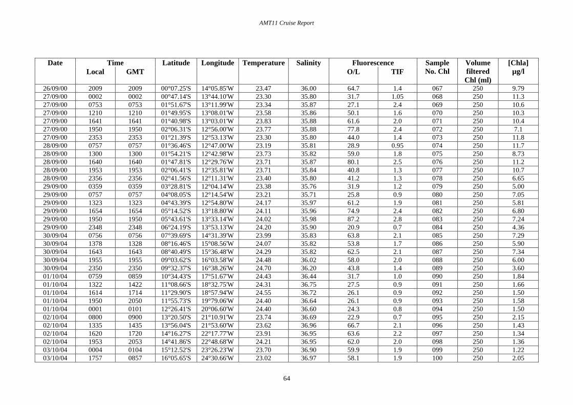
AMT11 Cruise Report

64

Time Fluorescence Date Local GMT

Latitude Longitude Temperature Salinity O/L TIF

Sample No. Chl

Volume filtered Chl (ml)

[Chla] µg/l

26/09/00 2009 2009 00°07.25'S 14°05.85'W 23.47 36.00 64.7 1.4 067 250 9.79 27/09/00 0002 0002 00°47.14'S 13°44.10'W 23.30 35.80 31.7 1.05 068 250 11.3 27/09/00 0753 0753 01°51.67'S 13°11.99'W 23.34 35.87 27.1 2.4 069 250 10.6 27/09/00 1210 1210 01°49.95'S 13°08.01'W 23.58 35.86 50.1 1.6 070 250 10.3 27/09/00 1641 1641 01°40.98'S 13°03.01'W 23.83 35.88 61.6 2.0 071 250 10.4 27/09/00 1950 1950 02°06.31'S 12°56.00'W 23.77 35.88 77.8 2.4 072 250 7.1 27/09/00 2353 2353 01°21.39'S 12°53.13'W 23.30 35.80 44.0 1.4 073 250 11.8 28/09/00 0757 0757 01°36.46'S 12°47.00'W 23.19 35.81 28.9 0.95 074 250 11.7 28/09/00 1300 1300 01°54.21'S 12°42.98'W 23.73 35.82 59.0 1.8 075 250 8.73 28/09/00 1640 1640 01°47.81'S 12°29.76'W 23.71 35.87 80.1 2.5 076 250 11.2 28/09/00 1953 1953 02°06.41'S 12°35.81'W 23.71 35.84 40.8 1.3 077 250 10.7 28/09/00 2356 2356 02°41.56'S 12°11.31'W 23.40 35.80 41.2 1.3 078 250 6.65 29/09/00 0359 0359 03°28.81'S 12°04.14'W 23.38 35.76 31.9 1.2 079 250 5.00 29/09/00 0757 0757 04°08.05'S 12°14.54'W 23.21 35.71 25.8 0.9 080 250 7.05 29/09/00 1323 1323 04°43.39'S 12°54.80'W 24.17 35.97 61.2 1.9 081 250 5.81 29/09/00 1654 1654 05°14.52'S 13°18.80'W 24.11 35.96 74.9 2.4 082 250 6.80 29/09/00 1950 1950 05°43.61'S 13°33.14'W 24.02 35.98 87.2 2.8 083 250 7.24 29/09/00 2348 2348 06°24.19'S 13°53.13'W 24.20 35.90 20.9 0.7 084 250 4.36 30/09/04 0756 0756 07°39.69'S 14°31.39'W 23.99 35.83 63.8 2.1 085 250 7.29 30/09/04 1378 1328 08°16.46'S 15°08.56'W 24.07 35.82 53.8 1.7 086 250 5.90 30/09/04 1643 1643 08°40.49'S 15°36.48'W 24.29 35.82 62.5 2.1 087 250 7.34 30/09/04 1955 1955 09°03.62'S 16°03.58'W 24.48 36.02 58.0 2.0 088 250 6.00 30/09/04 2350 2350 09°32.37'S 16°38.26'W 24.70 36.20 43.8 1.4 089 250 3.60 01/10/04 0759 0859 10°34.43'S 17°51.67'W 24.43 36.44 31.7 1.0 090 250 1.84 01/10/04 1322 1422 11°08.66'S 18°32.75'W 24.31 36.75 27.5 0.9 091 250 1.66 01/10/04 1614 1714 11°29.90'S 18°57.94'W 24.55 36.72 26.1 0.9 092 250 1.50 01/10/04 1950 2050 11°55.73'S 19°79.06'W 24.40 36.64 26.1 0.9 093 250 1.58 01/10/04 0001 0101 12°26.41'S 20°06.60'W 24.40 36.60 24.3 0.8 094 250 1.50 02/10/04 0800 0900 13°20.50'S 21°10.91'W 23.74 36.69 22.9 0.7 095 250 2.15 02/10/04 1335 1435 13°56.04'S 21°53.60'W 23.62 36.96 66.7 2.1 096 250 1.43 02/10/04 1620 1720 14°16.27'S 22°17.77'W 23.91 36.95 63.6 2.2 097 250 1.34 02/10/04 1953 2053 14°41.86'S 22°48.68'W 24.21 36.95 62.0 2.0 098 250 1.36 03/10/04 0004 0104 15°12.52'S 23°26.23'W 23.70 36.90 59.9 1.9 099 250 1.22 03/10/04 1757 0857 16°05.65'S 24°30.66'W 23.02 36.97 58.1 1.9 100 250 2.05

AMT11 Cruise Report

65

Time Fluorescence Date Local GMT

Latitude Longitude Temperature Salinity O/L TIF

Sample No. Chl

Volume filtered Chl (ml)

[Chla] µg/l

03/10/04 1321 1421 16°37.17'S 25°08.79'W 23.42 37.04 53.6 1.7 101 250 1.34 03/10/04 1633 1733 17°01.00'S 25°37.91'W 23.47 37.08 53.8 1.7 102 250 1.29 03/10/04 1949 2049 17°24.66'S 26°06.67'W 23.81 37.13 50.9 1.6 103 250 0.80 04/10/04 0003 0104 18°34.06'S 26°35.07'W 23.40 37.10 47.2 1.5 104 250 1.13 04/10/04 0757 0857 18°48.10'S 27°50.31'W 23.47 37.09 47.6 1.5 105 250 0.94 04/10/04 1352 1452 19°21.91'S 28°35.86'W 23.36 37.09 46.3 1.5 106 250 0.88 04/10/04 1649 1749 19°39.30'S 28°53.42'W 23.65 37.15 45.9 1.5 107 250 0.74 04/10/04 1943 2043 19°59.95'N 29°18.90'W 23.69 37.17 45.4 1.5 108 250 0.76 05/10/04 0004 0104 20°23.09'N 29°48.10'W 23.10 37.00 47.5 1.5 109 250 1.134 05/10/04 0753 0853 21°24.46'N 31°05.16'W 23.57 37.19 46.6 1.5 110 250 1.21 05/10/04 1317 1417 21°59.05'N 31°48.68'W 23.35 37.07 46.8 1.5 111 250 1.87 05/10/04 1626 1726 22°21.80'N 32°17.29'W 23.65 37.07 48.7 1.5 112 250 1.58 05/10/04 1955 2055 22°44.52'N 32°46.22'W 23.26 37.02 47.5 1.5 113 250 1.92 05/10/04 0001 0101 23°19.32'N 33°30.76'W 23.20 37.06 50.0 1.5 114 250 2.26 06/10/04 0759 0959 24°14.35'N 34°41.18'W 23.01 37.08 48.9 1.6 115 250 2.70 06/10/04 1333 1533 24°48.83'N 35°24.63'W 22.76 36.95 50.0 1.6 116 250 3.03 06/10/04 1645 1845 25°12.49'N 35°55.96'W 22.38 36.91 55.3 1.7 117 250 3.75 06/10/04 1950 2150 25°35.17'N 36°25.79'W 21.33 36.53 52.8 1.6 118 250 2.52 07/10/04 0011 0211 26°08.50'N 37°08.90'W 21.60 36.60 54.1 1.8 119 250 3.34 07/10/04 0753 0953 27°00.35'N 38°16.65'W 20.93 36.31 54.3 1.7 120 250 3.20 07/10/04 1357 1557 27°36.42'N 39°04.23'W 20.32 36.25 55.8 1.7 121 250 2.94 07/10/04 1426 1826 27°52.66'N 39°25.74'W 20.39 36.36 56.0 1.7 122 250 3.20 07/10/04 1957 2157 28°17.27'N 39°58.49'W 20.21 36.29 59.0 1.9 123 250 3.85 08/10/04 0002 0202 28°46.40'N 40°37.30'W 20.50 36.30 57.6 1.9 124 250 2.63 08/10/04 0753 0953 29°41.86'N 41°51.59'W 18.70 36.09 70.0 2.3 125 250 5.69 08/10/04 1322 1522 30°16.73'N 42°38.13'W 18.85 36.10 75.0 2.4 126 250 7.35 08/10/04 1631 1831 30°39.33'N 43°09.51'W 18.26 35.98 82.1 2.6 127 250 6.58 08/10/04 1948 2148 31°06.57'N 43°46.73'W 19.05 36.22 28.7 1.0 128 250 7.05 08/10/04 2348 0148 31°40.09'N 44°31.91'W 17.80 35.90 35.4 1.1 129 250 7.82 09/10/04 0754 1954 32°46.49'N 46°04.65'W 16.55 35.69 34.6 1.1 130 250 5.99 09/10/04 1400 1600 33°29.84'N 47°05.32'W 17.10 35.68 38.4 1.2 131 250 10.80