1

Cohort study

Atiporn Ingsathit MD.PhD.Section for Clinical Epidemiology & Biostatistics

Faculty of Medicine Ramathibodi HospitalMahidol University

Outlines

Definition of cohort study

How to assess risk

Survival analysis

2

Why we need observation studies?

Hypothesis generating Risk

Prognosis

Less expensive than RCT’s

Well done observation study yield results similar to RCT’s

Three questions to know the study design

Assign exposure/intervention? Experimental

Observational

Comparison groups ? Analytic

Descriptive

Start with exposure or outcome?

Case-control Cohort Cross-sectional

Clinical trials

Field trials

RCT

3

Cohort study: Marching towards outcomes

Population vs. cohort

Population All people in a defined setting or with certain

defined characteristics

Temporal and potentially dynamic

Cohort A population for whom membership is defined in a

permanent fashion

4

“Cohort” Group of soldiers that marched together into battle (Roman)

A group of people who share a commonexperience or condition A birth cohort shares the same year or period of birth

A cohort of smokers has the experience of smoking in common

A cohort of vegetarians share their dietary habit

Cohort study

An analytical, observational study, based on data, usually primary, from a follow-up period of a group in which some have had, have or will have the exposure of interest, to determine the association between that exposure and an outcome.

Do not provide empirical evidence that is as strong as that provided by properly executed randomized controlled clinical trials.

5

Cohort study

* Analytic study to find association between exposure and outcome

* Homogenous population

Exposure Outcome

Exposure & Outcome

Exposure Outcome

Risk factors

Intervention

Diseases

Health problems

Independent variable Dependent variable

6

Design

Type of cohort

Population Closed or fixed cohort

Opened or dynamic cohort

Design Retrospective

Prospective

Ambidirection

7

COHORT STUDIES

Fixed Cohort

Exposure

(+)

(-)

x

x

x

X = outcome

Relative risk = (2/3)/(1/3) = 2.0

Cumulative incidence

COHORT STUDIES

Dynamic Cohort

Exposure

(+)

(-)

Relative Risk

= 2/3/2/3 =1

or

2/5py/2/10py

= 2.0Years

XX

XX

Cumulative incidence or incidence rate

8

Designs

Prospective

Historic

Cohort study

Prospective cohort study

PopulationPeople without

The disease

Exposed

Not exposed

Disease

Disease

Direction of the study

No disease

No disease

Follow-up is mandatory*****

9

Cohort study

Retrospective cohort study

PopulationPeople without

The disease

Exposed

Not exposed

Disease

Disease

Direction of the study

No disease

No disease

Cohort study

Prospective Exposure, and factors

can be measured

Expensive, time consuming

Retrospective Cheaper Less time consuming Suitable for rare

outcome Some available data is

unavailable from historical part

Confounding factors

10

Study designs

Example

PopulationStudy

subject

Kidney Stone

No Stone

CKD

CKD

Direction of the study

Normal

Normal

Cohort Study Advantage

Can be standardized in eligible criteria & outcome assessment

Can establish temporal association

Disadvantage Usually expensive

Hard to blind

Long follow-up period for rare disorder

Difficult to find controls and confounders

11

What to look for in cohort studies

Who is at risk? Since women who have had a bilateral mastectomy

operation have almost no risk of breast cancer,17 they should not be included in cohort studies of CA breast.

Who is exposed? Cohort studies need a clear, unambiguous definition

of the exposure at the outset. This definition sometimes involves quantifying the exposure by degree, rather than just yes or no.

Who is an appropriate control (the unexposed)? The key notion is that controls should be similar to the

exposed in all important respects, except for the lack of exposure.

Have outcomes been assessed equally? Outcomes must be defined in advance; they should

be clear, specific, and measurable.

Keeping those who judge outcomes unaware of the exposure status of participants.

What to look for in cohort studies

12

Outcome measurement (1)

Subjective outcome

Fever Fever

PainPain

Objective outcome

HemocultureHemoculture

DeathDeath

Outcome measurement (2)

Surrogate outcome

Low-density lipoprotein

(LDL)

Low-density lipoprotein

(LDL)

ProteinuriaProteinuria

Clinical outcome

DeathDeath

ESRDESRD

13

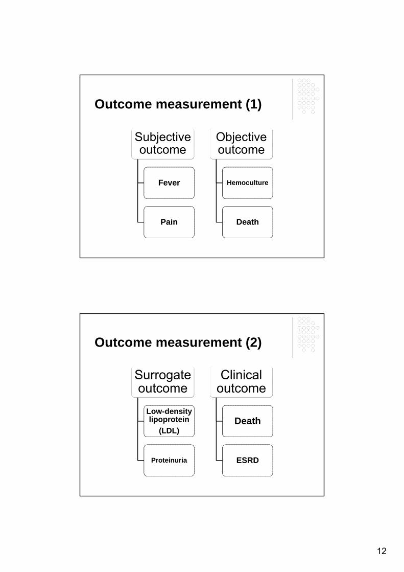
When should we use cohort design?

Key areas of inquiry in Clinical Epidemiology

Risk With what probability will disease occur?

Prognosis What are the outcomes from disease?

Diagnosis How good are the diagnostic tool?

Treatment How is the prognosis altered by treatment?

14

Onset of acute MI

Risk Prognosis Death

Risk factors

Age

Male

Smoking

HT

LDL

Inactivity

Prognostic factorsAgeFemaleSmokingHypotensionAnterior infarctionCHFVentricular arrhythmia

Cohorts and their purposes

Characteristic in common

To assess effect of

Example

Exposure Risk factor Lung cancer in people who smoke

Disease Prognosis Survival rate for patients with breast cancer

Preventive intervention

Prevention Reduction in incidence of pneumonia after pneumococcal vaccination

Therapeutic intervention

Treatment Improvement in survival for patients with Hodgkin’s disease given chemotherapy

15

How to assess risk or association?

Risk

The probability of some unexpected event.

The probability that people who are exposed to certain “risk factors” will subsequently develop a particular disease more often than similar people who are not exposed.

16

Risk factorsHypercholesterolemiaPositive family history

Valvular diseaseViral infection

SmokingDM

High blood pressure Congestive heart failure

Coronary atherosclerosisStroke

Renal failureMyocardial infarction

Multiple causes and effects

Way to express and compare risk

Expression Question Definition

Absolute risk What is the incidence of disease in a gr initially free of the condition?

I = #new case#People in group

Attributable risk(Risk difference)

What is the incidence of disease attributable to exposure?

AR = IE+-IE-

Relative risk(Risk ratio)

How many times more likely are exposed persons to become diseased, relative to nonexposed persons?

RR = IE+

IE-

Population-attributable risk

What is the incidence of disease in a population, associated with the prevalence of a risk factor?

ARp = AR x P

17

Exposure

Disease No disease

Total Stone CKD No CKD

Total

+ a b a+b Yes 80 10 90

- c d c+d NO 20 90 110

a+c b+d n 100 100 200

Term General Example Question?

Risk a/(a+b)

Orc/(c+d)

80/90

Or20/110

What is the incidence of disease in a group initially free of the condition?

Relative risk a/(a+b) c/(c+d)

80/90 20/110= 5

How many times more likely are exposed persons to become disease, relative to nonexposed persons?

Way to express and compare risk

Exposure

Disease No disease

Total Stone CKD No CKD

Total

+ a b a+b Yes 80 10 90

- c d c+d NO 20 90 110

a+c b+d n 100 100 200

Term General Example Definition

Attributable risk (AR)

a/(a+b) –c/(c+d)

80/90 – 20/110= 0.7

The incidence of disease attributable to exposure

Population attributable risk

PAR= ARxPEX

AR x (a+b)/n

0.7 x 90/200= 0.32

The incidence of disease in a population is associated with the occurrence of a risk factor

Way to express and compare risk

18

Relative risk vs. attributable risk

RR

The strength of association

Causal inference

Valuable in etiologic studies

AR

Measure of how much of the disease risk is attributable to a certain exposure

Valuable in clinical practice and public health

Incidence

population unexposed

Ipop - I unexposed

Population attributable risk (PAR)

PAR% = {(Ipop - I unexposed ) / Ipop}100

19

Incidence

population unexposed

Ipop - I unexposed

Population attributable risk (PAR)

PAR% = {(Ipop - I unexposed ) / Ipop}100

If we had an effective prevention program (stop stone) in this population, how much of a reduction in CKD incidence could we anticipate in the total population (of both stones and no stones)?

Incidence rate

The measure of disease in cohort studies is the incidence rate, which is the proportion of subjects who develop the disease under study within a specified time period.

The numerator of the rate is the number of diseased subjects.

the denominator is usually the number of person-years of observation.

20

Total observed person-time 69.1 mo.

Survival analysis The likelihood that patients with a given

condition will experience an outcome at any point in time.

Cohort or a randomized control trial Time to event

Origin End point

21

Why survival analysis? Investigators Frequently must analyze

their data before all the subjects have died or the event has occurred.

Why survival analysis? Investigators frequently must analyze

their data before all the subjects have died or the event has occurred.

The patients do not typically enter the study at the same time.

22

Total observed person-time 69.1 mo.

Survival analysis Event : Code 1 0

1= Event occurred : death

0= censored observation: alive orloss to follow-up

Censored observation: An observation whose value is unknown because the subject has not been in the study long enough for the outcome of interest to occur

23

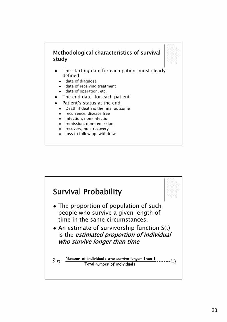
Methodological characteristics of survival study

The starting date for each patient must clearly defined

date of diagnose date of receiving treatment date of operation, etc.

The end date for each patient Patient’s status at the end Death if death is the final outcome recurrence, disease free infection, non-infection remission, non-remission recovery, non-recovery loss to follow up, withdraw

Survival Probability The proportion of population of such

people who survive a given length of time in the same circumstances.

An estimate of survivorship function S(t) is the estimated proportion of individual who survive longer than time

24

Life table analysis

ni wi di qi=

di/[ni-(wi/2)]

Pi=1-qi Si=pi(pi-1)

Interval start time

(mo)

No entering this interval

No withdrawal during interval

No of terminal events

Proportion terminating

Proportion surviving

Cum proportion surviving at End

0 13 2 1 0.083 0.917 0.917

3 10 4 1 0.125 0.875 0.802

6 5 4 0 0 1.000 0.802

9 1 1 0 0 1.000 0.802

Kaplan-Meier method ni Ci di qi= di/ni Pi=1-qi Si=pi(pi-1)

Event time

(mo)

No at risk Censor No of events

Mortality Survival Cum survival

3 10 0 1 1/10=0.1 0.90 0.9

4 9 1 0 0/9=0 1.0 0.9*1=0.9

5.7 8 1 0 0/8=0 1.0 0.9*1*1=0.9

6.5 7 0 2 2/7= 0.28 0.72 0.9*1*1*0.72=0.648

.

10

25

Kaplan-Meier survival estimate

Hazard function Hazard function h (t) is the probability

that an individual will die (fail) at time t. The death rate for an individual surviving

at time t. The cumulative hazard (H(t)) is therefore

the convergence of cumulative survival S(t), which is the probability that an individual would die after time t.

26

Comparing two survival curves Logrank test The null hypothesis for comparing

survival/failure times is:

Logrank statistic for survival No of patients at risk in Gr1 Gr2

No of observed events in Gr1 Gr2

No of expected events in Gr1 Gr2

χ 2 = (O1-E1)2 + (O2-E2) 2

E1 E2

27

Time(month)

d1jNumber ofDeaths

n1jNumber

at risk

d2j n2j dj nj e1j e2j

.03

.07.1.17.23.27.503.035.939.139.8013.2315.83

1111111101100

1514131211109877655

0000000010011

15151515151515151514141413

1111111111111

30292827262524232221201918

1x15/30=.501x14/29=.481x13/28=.46

.44

.42

.40

.38

.35

.32

.33

.30

.26

.28

1x15/30=.501x15/29=.521x15/28=.54

.56

.57

.60

.63

.65

.68

.67

.70

.74

.72

Total 10O1

3O2

4.93E1

8.07E2

Demonstrating calculation of Log-rank statistics

P=0.001

Hazard ratio HR = O1/E1

O2/E2

= 10/4.93 = 2.03/0.37 = 5.53/8.07

The risk of GF at any time in recipients olderthan 50 years old is 5.5 times greater than the riskin recipients who younger.

Faster

28

CC-EBM

stsum, by(ager_gr) failure _d: GF == 1 analysis time _t: _t id: hnr

| incidence no. of |------ Survival time -----| ager_gr | time at risk rate subjects 25% 50% 75% ---------+--------------------------------------------------------------------- <50 | 831.5701574 .0865832 253 3.756331 6.652977 . >=50 | 229.7221081 .0740025 71 3.635866 . . ---------+--------------------------------------------------------------------- total | 1061.292266 .08386 324 3.635866 . .

. sts test ager_gr failure _d: GF == 1 analysis time _t: _t id: hnr

Log-rank test for equality of survivor functions

| Events Events ager_gr | observed expected --------+------------------------- <50 | 72 69.61 >=50 | 17 19.39 --------+------------------------- Total | 89 89.00

chi2(1) = 0.38 Pr>chi2 = 0.5391

Statistical analysis

Survival analysis with Kaplan-Meier was used to estimate survival rate, median survival time of recipients.

Log-rank test was used to compare survival curves

Cox regression was used to determine factors associated with survival time

29

Cox regressionProportional hazard model The Cox proportional hazard model (or Cox

regression) was proposed by Cox in 1972 and has been used widely since then when desiring to investigate several variables simultaneously for time to event outcomes.

The model is a semi-parametric approach –no particular type of distribution is assumed for survival times.

Cox regressionProportional hazard model A strong assumption The effects of the different groups of

variable on survival are constant over time.

Benefits of the Cox model are: (i) It can perform multiple comparisons (ii) It’s able to adjust for confounding

variables for which the study design can not control for.

30

Example

Materials and Methods We examined a cohort of consecutive

end-stage renal disease patients who underwent first kidney transplantation at a single-center, university-based hospital during a 6- year study period. All subjects had a follow-up of at least 6 months.

31

Materials & Methods

Setting

The study was conducted at Ramathibodi Hospital which is a 1200-bed university hospital in Bangkok.

Study design

Ambidirectional cohort study

Methods Study design A ambidirectional cohort studyPast Present Future

Start 1997 2002 2006

32

Materials & Methods

Study population Inclusion criteria

Medical records of patients aged at least 18 years old who initially had undertaken kidney transplantation in Ramathibodi Hospital

Exclusion criteria

Multi-organ transplants or dual kidney transplants

Recipient who had graft failure or death within 6 months

Recipients who had time of follow-up of less than 6 months

Study design

HBV HCVHBV

HCV

Non HBVHCV

Follow over time

GF

No GF

GF

No GF

GF

No GF

33

Outcome The primary outcomes were time to graft

failure.

Graft failure was defined by the introduction of long-term dialysis after transplantation or retransplantation.

Statistical analysis Graft and patient and survivals were

determined using the Kaplan-Meier method.

Log-rank test was used to compare survival curves

Cox regression analysis with time-varying covariates was used to assess the effect of HBV/HCV infections adjusting for confounders.

34

Data collection

Baseline data Follow-up data

Baseline dataTime-fixed covariates

Origin End of study

35

Baseline dataTime-fixed covariates

Origin End of study

Follow-up dataTime-dependent covariates

Graft survival Patient survival

P=0.001 P=0.003

Among 353 recipients: HBV+ 6.5%, HCV+ 6.2%

36

Incidence of graft failure and HR

Characteristics No. ofGF

Totalsubjects

Timeat risk(years)

IncidenceGF/100/year

Hazard ratio(95%CI)

P-value

Recipient age, years < 50 > 50

920

26477

272.56981.12

3.302.01

1.0***1.67(0.76-3.68)

0.20

SexMaleFemale

1019

131210

461.93791.75

2.162.40

1.0***1.10(0.50-2.33)

0.84

Duration of dialysis <12 months

>12 months1415

162161

623.69551.88

2.242.71

1.0***1.17(0.56-2.43)

0.66

Anti-HCVPositiveNegative

623

22319

90.331171.7

7.331.96

3.88(1.57-9.57)1.0***

0.001

Potential bias in cohort studies

Selection bias Susceptibility bias

Migration bias

Measurement bias

Survival cohorts

Confounders

37

Selection or Susceptibility bias Groups being compared are not equally

susceptible to the outcome of interest, other than the factor under study

CA colon : CEA level and Relapse

Dukes classification and Relapse

Methods for controlling selection bias

MethodPhase of study

Design Analysis

Randomization +

Restriction +

Matching +

Stratification +

Adjustment

Multivariable

+

38

Propensity score matching (PSM)

A statistical matching technique that attempts to estimate the effect of a treatment, policy, or other intervention by accounting for the covariates that predict receiving the treatment.

PSM attempts to reduce the bias due to confounding variables that could be found in an estimate of the treatment effect obtained from simply comparing outcomes among units that received the treatment versus those that did not.

Propensity score matching (PSM)

For observational studies, the assignment of treatments to research subjects is typically not random.

Matching attempts to mimic randomization by creating a sample of units that received the treatment that is comparable on all observed covariates to a sample of units that did not receive the treatment.

39

PSM procedure

1.Run logistic regression: Dependent variable: Y = 1, if participate; Y = 0, otherwise.

Choose appropriate confounders (variables hypothesized to be associated with both treatment and outcome)

Obtain propensity score: predicted probability (p) or log[p/(1 − p)].

2. Check that propensity score is balanced across treatment and comparison groups, and check that covariates are balanced across treatment and comparison groups within strata of the propensity score.

3.Match each participant to one or more nonparticipants on propensity score

40

Baseline characteristics

Results

41

Migration bias

HBV HCVHBV

HCV

Non HBVHCVFollow over time

GF

No GF

GF

No GF

GF

No GF

Drop out

Cross over

Best-case/worst case analysis

Measurement bias

When patients in one subgroup of a cohort stand a better chance of having their outcomes detected than another subgroup.

Ways to control Unawareness of person who record outcome

events

Set up strict criteria/rules for diagnose outcome events

Apply efforts to discover outcome events equally

42

Survivor bias

Tracking participants over time

Have losses been minimised?

True cohortObserved

improvementTrue

improvement

Assemble cohortN=150

Measure outcomeImproved: 75Not improved: 75

50% 50%

Survival cohort

Begin F/UN=50

Not observedN=100

Measure outcomeImproved: 40Not improved: 10

DropoutsImproved: 35Not improved: 65

80% 50%

43

Confounding A factor that distorts the true

relationship of the study variables of interest by being related to the outcome of interest.

X Y

W

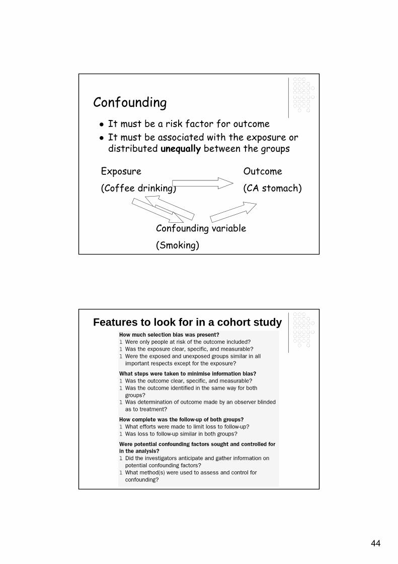
Confounding It must be a risk factor for outcome It must be associated with the exposure or

distributed unequally between the groups

Exposure

(Coffee drinking)

Outcome

(CA stomach)

44

Confounding It must be a risk factor for outcome It must be associated with the exposure or

distributed unequally between the groups

Exposure

(Coffee drinking)

Outcome

(CA stomach)

Confounding variable

(Smoking)

Features to look for in a cohort study

45

Conclusion

Cohort studies done well can generate similar results as RCT’s, and some questions cannot answered by RCT’s.

Appreciate the strengths and weakness of cohort studies.