ATIKOKAN MINE CENTRE Ontario Airborne Magnetic and

Report on Atikokan-Mine Centre Area Geophysical Survey

Geophysical Data Set 1029

ATIKOKAN MINE CENTREOntario Airborne Magnetic and Electromagnetic Surveys


Processed Data and Derived ProductsArchean and Proterozoic “Greenstone” Belts

Ontario Geological SurveyMinistry of Northern Development and MinesWillet Green Miller Centre933 Ramsey Lake RoadSudbury, Ontario, P3E 6B5Canada



2

TABLE OF CONTENTS PageCREDITS........................................................................................................................................ 3DISCLAIMER ................................................................................................................................ 4CITATION...................................................................................................................................... 41) INTRODUCTION ................................................................................................................ 52) FLIGHT PATH REPROCESSING ...................................................................................... 8

2.1) Flight Path Standards ..................................................................................................... 82.2) Flight Path Reprocessing Methodology ......................................................................... 8

3) ALTIMETER DATA REPROCESSING ........................................................................... 104) MAGNETIC DATA REPROCESSING............................................................................. 11

4.1) Editing of Magnetic Data .......................................................................................... 124.3) Micro-Levelling ........................................................................................................... 124.4) Levelling to Ontario Master Aeromagnetic Grid ......................................................... 144.5) Gridding of Reprocessed Magnetic Data ..................................................................... 164.6) Second Vertical Derivative of the Total Magnetic Field ............................................. 164.7) Keating Correlation Coefficients................................................................................... 17

5) ELECTROMAGNETIC DATA REPROCESSING........................................................... 195.1) Reprocessing Specifications and Tolerances ............................................................ 205.2) Electromagnetic Data Corrections ............................................................................... 215.3) Decay Constant Calculation ......................................................................................... 265.4) Apparent Resistivity Calculation ................................................................................. 285.5) Correction for Asymmetry (Deherringboning) ............................................................ 315.6) Updated EM Anomaly Database.................................................................................. 32

6) QUALITY CONTROL AND QUALITY ASSURANCE.................................................. 356.1) Flight Path.................................................................................................................. 356.2) Profile Data................................................................................................................. 356.3) Grid Data ................................................................................................................... 366.4) EM Anomaly Data..................................................................................................... 37

7) SURVEY SPECIFIC DETAILS - ATIKOKAN MINE CENTRE..................................... 387.1) Flight Path Reprocessing ........................................................................................... 387.2) Altimeter Data Reprocessing ....................................................................................... 397.3) Magnetic Data Reprocessing........................................................................................ 397.4) Electromagnetic Data Reprocessing............................................................................. 427.5) Known Data Bugs ........................................................................................................ 47

REFERENCES ............................................................................................................................. 48APPENDIX A............................................................................................................................... 49

SURVEY HISTORY ............................................................................................................ 49APPENDIX B ............................................................................................................................... 53

CONTENTS OF PROFILE, GRID, KEATING AND ELECTROMAGNETIC ANOMALYDATABASES ....................................................................................................................... 53

APPENDIX C ............................................................................................................................... 582002 DIGITAL ARCHIVE RE-FORMATTING NOTES ................................................... 58



3

CREDITS

The overall project management, scientific authority and quality control was provided by Vinod

K. Gupta, Ontario Geological Survey, Sudbury, Ontario.

The following is a list of the organisations that have participated in this project, and their various

responsibilities:

Paterson, Grant & Watson Limited, Toronto - Prime contractor

-project management

-magnetic data processing

Geoterrex, a division of CGG Canada Ltd., Ottawa - Sub-contractor

-flight path correction

-electromagnetic data processing (time-domain surveys)

Dighem/I-Power, a division of CGG Canada Ltd., Mississauga - Sub-contractor

-flight path correction

-electromagnetic data processing (frequency-domain surveys)

CGI Controlled Geophysics Inc., Thornhill - Sub-contractor

- quality control of data

- data merging and preparation of final products



4

DISCLAIMER

Every possible effort has been made to ensure the accuracy of the information provided on this

CD-ROM; however, the Ontario Ministry of Northern Development and Mines does not assume

any liability or responsibility for errors that may occur. Users may wish to verify critical

information.

CITATION

Information about the Archean and Proterozoic “greenstone belts” airborne geophysics digital

data set may be quoted if credit is given. It is recommended that reference be made in the form

shown in this example:

Ontario Geological Survey 2003. Ontario airborne geophysical surveys, magnetic

data, Atikokan-Mine Centre area; Ontario Geological Survey, Geophysical Data

Set 1029.



5

1) INTRODUCTION

High resolution airborne magnetic and electromagnetic surveys, over major greenstone belts,

were initiated in 1975 by the Ontario Department of Mines (currently known as the Ontario

Geological Survey) to aid geological mapping and mineral exploration. Between the period

1975 to 1992, thirty-two airborne surveys were flown and processed by different survey

contractors and subcontractors. The two earlier surveys, Matachewan and Bamaji-Fry Lakes,

were acquired in analog form and the remaining thirty surveys were recorded digitally. The

surveys were flown at a nominal flight line spacing of 200m with the exception of James Bay

Cretaceous Basin survey, which was flown at a flight line spacing of 1000m. The flight

directions for the surveys, including individual survey blocks, were chosen to transect the

predominant regional structural trends of the underlying rocks. The result of the surveys were

published on 1:20,000 semi-controlled photo mosaic paper maps, showing total magnetic field

contours onto which picked electromagnetic conductor anomalies were superimposed in symbol

form.

There are significant differences in quality of data acquisition, and original processing, of

olderand newer surveys. The surveys flown recently were designed and flown based on the

state-of-the-art specifications, equipment and technology, while some of the older surveys,

though conducted to the then industry prevailing standards, were poorly processed. In many

cases, on older surveys, the local map coordinates were registered in map inches of uncontrolled

to semi-controlled photo mosaics. The vast amount of digital data, collected by the survey

contractors,was archived on 9-track tapes of different sizes and densities, in numerous

incompatible data formats and file structures, many of which were difficult to access. For this

reason the archival digital data largely remained inaccessible to the mining industry.

To alleviate many of these problems, and to bring the archival data set of all thirty-two airborne

magnetic and electromagnetic (AMEM) surveys to modern data storage, digital processing and



6

interpretation standards, the present recompilation and reprocessing project was initiated under

the Northern Ontario Development Agreement (NODA). This includes approximately 450 000

line-km of AMEM data, which was recompiled and reprocessed to correct any errors in the

original data sets, to compute new derived products and to produce a revised electromagnetic

anomaly database, using state-of-the-art geophysical data processing and imaging techniques.

The major objectives of this project were to:

1) Provide a single, well-defined, common data format for all thirty-two AMEM

survey data sets on CD-ROM, allowing easy access to the data on a PC platform.

2) Digitize survey data acquired in analog form, obtain missing or bad data from

digital or paper archives, and check the validity of all data including units,

conversion factors, etc.

3) Analyse and correct errors in the flight path to account for distortions in the

photomosaics and provide a digital flight path referenced to Universal Transverse

Mercator (UTM) coordinates.

4) Link and level all thirty-two surveys total magnetic field data to the Single Master

Aeromagnetic Grid for Ontario, which was prepared from the Geological Survey

of Canada’s magnetic database under an earlier project.

5) Reprocess the magnetic data to provide image quality total magnetic field grids

and profiles for each survey.

6) Create image quality second vertical derivative grids of the total magnetic field.



7

7) Compute image quality apparent resistivities from a selected single frequency of

the frequency-domain electromagnetic data, which have been fully corrected for

signal to noise enhancement and accurately levelled.

8) Compute image quality decay constant and resistivity values from the corrected

and levelled data channels of time-domain electromagnetic data (INPUT,

GEOTEM I and GEOTEM II systems). Provide de-herringboned (i.e. correct for

directional effect) decay constant and resistivity grids for all time-domain

surveys.

9) Re-pick electromagnetic anomalies from the surveys in a consistent manner, and

store anomaly parameters, including a unique identifier, in a new digital anomaly

database.

The resulting profile and grid data in digital form, along with the second vertical

derivative of the total magnetic field, the apparent resistivity and decay constant values,

and a comprehensive EM anomaly database, will become valuable tools for orebody

detection, and enhanced lithological and structural mapping of the geology. The original

profile data are also included in the profile database for reference. A full description of

the digital databases are provided in Appendix B. In addition, MNDM has archived a

number of interim processed channels, which can be made available to users on request.



8

2) FLIGHT PATH REPROCESSING

2.1) Flight Path Standards

The goals of the flight path processing were to satisfy the three criteria below:

1) The database coordinates of picked fiducial points corresponding to identifiable

topographic features on the photo mosaic should match the position of these features on

published topographic maps within 100 metres on average.

2) The appearance of the final levelled total magnetic field and apparent resistivity data is

consistent with the above standard of accuracy, i.e. continuity of linear features on

adjacent flight lines to within 100 metres on average.

3) Speed checks run on the profile data do not show discontinuities or improbable values for

the survey aircraft flight speed.

2.2) Flight Path Reprocessing Methodology

The following steps were taken to ensure that the final flight path data is in correct UTM

coordinates:

1) Determine, if necessary, a regional correction comprising scaling, rotation and

translation based on position of flight path relative to identifiable topographic features

on the uncontrolled photo-mosaics.

2) Apply any regional correction to the digital data.



9

3) Plot the digital flight path (with regional correction) at the 1:20,000 scale.

4) Pick visual control points from the published survey maps at identifiable topographic

features. Transfer these pick points to a scale stable 1:20,000 scale topographic map

(Ontario Base Map), or if not available, to a 1:50,000 scale topographic map

(National Topographic System).

5) Identify the pick points on the digital flight path. Digitise the vectors joining the pick

points on the digital flight path to the visual pick points on the topographic maps.

These vectors represent the required corrections at each pick point.

6) Generate a polynomial surface through the corrections for each of the easting and

northing components of the digitised vectors.

7) Correct the regionally accurate digital flight path for local distortions by adding the

polynomial surfaces, which define the corrections, to the digital data.

8) Plot the final corrected flight path at 1:20,000 and confirm that all control points have

been properly corrected.

9) Verify the flight path positioning by correlating the geophysical responses to any

identifiable cultural features.

The error of the final flight path position is within the specification of less than 100m. The

primary source of error is the visual picking of the control points.

The final corrected flight path is provided in the archive.



10

3) ALTIMETER DATA REPROCESSING

The altimeter data has been checked for spikes, negative values, discontinuities, and other errors,

in order to ensure a correct contribution to the computation of the apparent resistivity values (see

Section 5 Electromagnetic Data Reprocessing).

The following steps were taken to correct any errors in the altimeter data:

1) The data set was checked to ensure that it represents the distance in metres from the ground

to the EM system. In many surveys, the data set required a correction to account for the

difference in elevation between the altimeter equipment and the EM equipment. Most

surveys required a conversion from imperial to metric units of measurement.

2) The data set was viewed on a line by line basis to check for errors using either a profile editor

or digital profile maps.

3) Any spikes were replaced with default values. The default values were subsequently

interpolated using a modified cubic spline (Akima, 1970).



11

4) MAGNETIC DATA REPROCESSING

The final magnetic data sets are image quality and conform to the criteria described below. All

reprocessing corrections (Chart 4.1) are incorporated into the profile data as well as the final

grids.



12

4.1) Editing of Magnetic Data

The original magnetic profiles were viewed and edited for spikes, discontinuities, or other noise

attributable to problems with the measuring and recording instruments and/or digitizing errors.

The original and edited values are each retained in a separate column in the profile database.

4.2) IGRF Removal

An IGRF grid was calculated for the survey area and year based on coefficients supplied by the

United States National Geophysical Data Center. The IGRF grid was calculated at 1 km cell size

and then extracted to the profile data using cubic spline interpolation between grid points. The

extracted IGRF values were then subtracted from the magnetic data values to give the IGRF

corrected profile data. Both the IGRF values and the IGRF corrected survey data are stored in

the magnetic profile database.

4.3) Micro-Levelling

Micro-levelling (Minty, 1991) was applied to remove low-amplitude flight line noise that

remained in the magnetic data after tie line levelling by the original survey contractor. In this

process a level correction channel is calculated and added to the profile database. This

correction is then subtracted from the original data to give a set of levelled profiles, from which a

levelled grid may then be generated. Micro-levelling has the advantage over standard methods

of decorrugation that it better distinguishes flight line noise from geological signal, and thus can

remove the noise without causing a loss in resolution of the data. Noise due to flight line level

drift has been removed so that the background level of line noise visible in magnetically quiet

areas is no more than: 1 nT for surveys flown from 1985-1991, 3 nT for 1978-1984 surveys, or 5

nT for 1975-1977 surveys, and similarly the background level of line noise in the second vertical



13

derivative grids is no more than 0.001 nT/m2 for any survey. The micro-levelling process is

described below.

First the edited and IGRF-corrected profile data is gridded, with a cell size equal to 1/5 of the

flight line spacing. Then a directional high-pass filter is applied in the Fourier-domain, to

produce a grid known as the decorrugation noise grid, since it contains the noise to be removed

from the data for decorrugation purposes. The decorrugation noise filter is a sixth-order high-

pass Butterworth filter with a cutoff wavelength of four times the flight line spacing, combined

with a directional filter. The directional filter coefficient as a function of angle is F = sin 2 a,

where a is the angle between the direction of propagation of a wave and the flight line direction

(i.e. F=0 for a wave travelling along the flight lines, and F=1 for a wave travelling perpendicular

to them). This is the opposite of what is usually called a decorrugation filter, since the intention

here is to pass the noise only, rather than reject it.

The decorrugation noise grid will contain the line level drift component of the data, but it will

also contain some residual high-frequency components of the geological signal. Flight line noise

appears in the decorrugation noise grid as long stripes in the flight line direction, whereas

anomalies due to geological sources appear as small spots and cross-cutting lineaments,

generally with a higher amplitude than the flight line noise, but with a shorter wavelength in the

flight line direction. The noise and the geological signal can be separated on the basis of these

two criteria, i.e. amplitude and wavelength in the flight line direction. The operator examines the

noise grid and estimates the maximum amplitude and minimum wavelength of the flight line

noise. The noise grid is then extracted as a new channel in the database. Next, amplitude

limiting is applied to this channel, such that any values exceeding the estimated maximum

amplitude of the flight line noise are set to zero. Finally, the amplitude-limited noise channel is

filtered with a Naudy non-linear low-pass filter (Naudy and Dreyer, 1968). The filter width is set

so that any features narrower than half the estimated minimum wavelength of the flight line

noise are eliminated.



14

What remains at the end of all these filtering steps should be the component of line level drift

only. This is then subtracted from the original data to give a better levelled set of profiles.

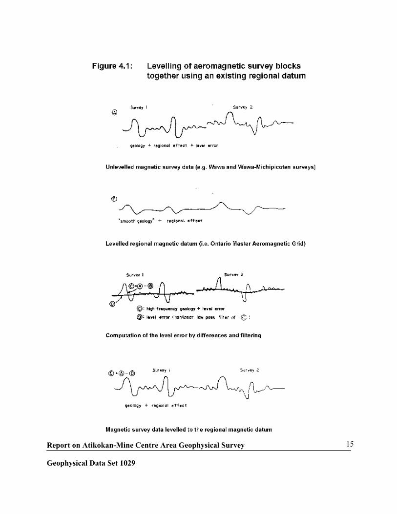
4.4) Levelling to Ontario Master Aeromagnetic Grid

The magnetic data is adjusted to the base level of the Ontario Master Aeromagnetic Grid, a

linked and levelled magnetic reference grid at 200 m cell size and 300 m drape height for all of

Ontario (Reford et al., 1990; Gupta et al. 1989). This has been done for the sake of consistency,

so that adjacent surveys can be linked together seamlessly, and all of the survey data from this

project can be conveniently linked with existing magnetic survey coverage in other areas. The

base-level adjustment was applied as follows: The survey data was gridded at 200 m cell size

and upward continued to 300 m observation height to match the Ontario grid. The difference of

the two grids was computed, and then smoothed with a 15-km-wavelength low-pass filter. This

low-frequency difference grid was then extracted to the profile database and subtracted from the

original survey data values, to bring the survey to the same base level as the Ontario grid. Figure

4.1 shows how two adjacent surveys can be linked by adjusting them both to the base level of the

master aeromagnetic grid. After the base shift has been applied, the reprocessed magnetic

profiles and grids are still effectively at the same observation height as the original data, so that

no resolution is lost.



15



16

4.5) Gridding of Reprocessed Magnetic Data

For most surveys the reprocessed total field magnetic grid was calculated from the final

reprocessed profiles by a minimum curvature algorithm (Briggs, 1974). The accuracy standard

for gridding is that the grid values fit the profile data to within 1 nT for 99.98% of the profile

data points. The average gridding error is well below 0.1 nT.

Minimum curvature gridding provides the smoothest possible grid surface that also honours the

profile data. However, sometimes this can cause narrow linear anomalies cutting across flight

lines to appear as a series of isolated spots.

Trend-enhanced gridding interpolates data values between flight lines so as to join up local

maxima on adjacent lines, and similarly, to join local minima, so that geological trends are

shown clearly. This has the great advantage over other methods of trend enhancement that it

reinforces identifiable trends going in any direction, rather than merely in one single favoured

direction. Similar to the conventional minimum-curvature gridding, trend-enhanced gridding

also fits the profile data values within 1 nT for 99.98% of the data points. The only differences

are in the values assigned to grid points between flight lines.

4.6) Second Vertical Derivative of the Total Magnetic Field

The second vertical derivative of the total magnetic field was computed to enhance small and

weak near-surface anomalies and as an aid to delineate the contacts of the lithologies having

contrasting susceptibilities. The location of contacts or boundaries is usually traced by the zero

contour of the second vertical derivative map.

The original second vertical derivative grids had been calculated and filtered with an optimum

Weiner filter in order to suppress noise. However, a loss of precision, resulting from the storage



17

format of the grid was noticed and the second vertical derivative grids were recalculated. The

second vertical derivative filter was applied along with a Butterworth filter. The Butterworth

filter parameters were chosen after applying a range of values and inspecting the resulting grids.

The best result, in which noise was adequately suppressed without undue degradation of

geological signal, was obtained using a wavelength of 200m and a degree of 8.

The Butterworth filter is described by the following expression:

where:

k0 is the central wavenumber of the filter

n is the degree of the filter function

For each survey area, the shaded relief images of the second vertical derivative map were also

used to identify and assess flight line noise contents of the micro-levelled total magnetic field

grids.

4.7) Keating Correlation Coefficients

Possible kimberlite targets have been identified from the residual magnetic intensity data, based

on the identification of roughly circular anomalies. This procedure was automated by using a

known pattern recognition technique (Keating, 1995), which consists of computing, over a

moving window, a first-order regression between a vertical cylinder model anomaly and the

gridded magnetic data. Only the results where the absolute value of the correlation coefficient is

above a threshold of 75% were retained. The results are depicted as circular symbols, scaled to

reflect the correlation value. The most favourable targets are those that exhibit a cluster of high

amplitude solutions. Correlation coefficients with a negative value correspond to reversely

+

=

0

1

)(1

kk

kLn



18

magnetized sources. It is important to be aware that other magnetic sources may correlate well

with the vertical cylinder model, whereas some kimberlite pipes of irregular geometry may not.

The cylinder model parameters are as follows

Cylinder diameter: 200 m

Cylinder length: infinite

Overburden thickness : 5 m

Sensor height: 120 m

Magnetic inclination: 76.55o N

Magnetic declination: 1.0o W

Magnetization scale factor: 100

Maximum data range: 1 000 nT

Number of passes of smoothing filter: 0

Model window size: 15

Model window grid cell size: 40 m



19

5) ELECTROMAGNETIC DATA REPROCESSING



20

5.1) Reprocessing Specifications and Tolerances

- EM filtering and processing techniques were applied to the data to reduce noise,

improve base level estimates and increase the signal to noise ratio of selected EM

profile data channels for the purpose of obtaining reliable and unambiguous

resistivity and decay constant calculations;

- corrected amplitudes for those EM channels which were selected for resistivity

calculations were to be near zero when no conductive or permeable source was

present;

- due to high costs of removal, the cultural effects were to be left intact in the EM

datasets;

- the EM data were to be checked and corrected for residual spheric and other

identifiable noise events;

- for INPUT datasets, the EM channels were to be levelled to the following

specifications:

± 200 ppm on channel 1, ± 50 ppm on channel 6 and pro-rated for in-between channels.

- for GEOTEM datasets, the EM channels were to be levelled to the following

specifications:

± 75 ppm on channel 1, ± 25 ppm on channel 12 and pro-rated for in-between channels.



21

5.2) Electromagnetic Data Corrections

Correction for Spherics:

All recognizable artifacts caused by spheric activity were removed from the channel data by

interpolation, utilizing a graphics screen.

Base Level Corrections:

Base levels for every channel were reviewed and adjusted when necessary by viewing the data in

profile form on a graphic screen. Based on the resistive segments along each line (when noted),

an appropriate combination of tilt and/or dc offset was applied to each channel baseline to set the

mean value of the resistive sections of the data to zero. The accuracy of the resulting baseline

values will still oscillate within the envelope of the original noise level for each channel, but

these variations in the true amplitude level are taken into account during the calculation of the

resistivity and decay constant values by appropriate application of thresholds and weighted

fitting of the data.

Figure 5.1 illustrates the resulting decay constant traces from the channels before and after the

adjustment of the baselines within the noise envelope thresholds, as specified in section 5.1. The

good agreement between the two traces indicate that the application of the threshold and

weighted fitting during the decay constant calculation can effectively compensate for residual

baseline deviations which are within the noise envelope of the data.



22



23

Filtering of the EM Channels:

Residual noise on the data was removed by applying a time domain adaptive filter which

switches between a light and heavier filtering weight based on local gradient change. In areas of

anomalous response, filtering was aimed at wavelengths of 1 Hz and higher; in the background,

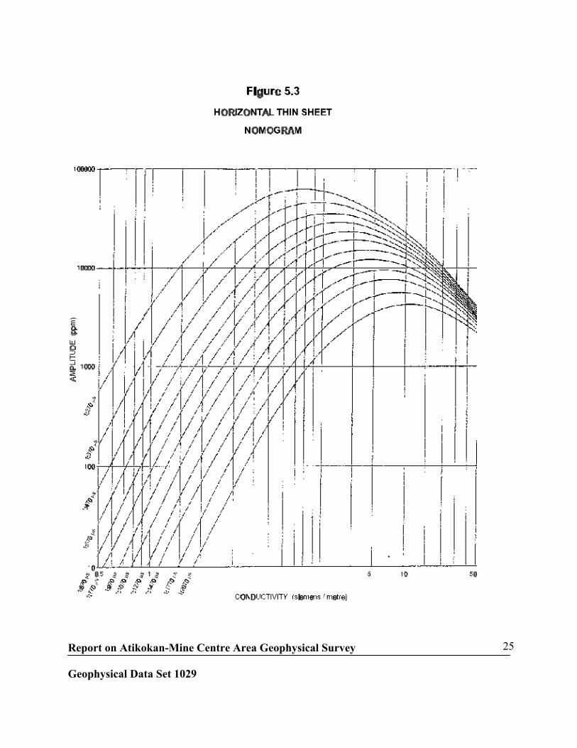
more resistive areas, the wavelength cut-off was set at 0.33 Hz and higher. Figures 5.2 and 5.3

provide an example of the effect of the filtering.



24



25



26

Final Data Acceptance:

Interim digital archives of the raw and reprocessed data (in line form) and all the derived EM

grids underwent initial quality control. The total effect of the reprocessing steps applied to the

data (explained above) can be verified by creating difference traces between the original

recovered data and the reprocessed data. Sample profile plots were also plotted as quality

control measures to display the original recovered EM data and the reprocessed data.

5.3) Decay Constant Calculation

By definition, the INPUT system is a time domain system (TDEM) which measures the rate of

decay of the received secondary field through the use of discrete time gates positioned during the

off-time. The most direct representation of this information is by the decay constant (Vaughan,

1988) which is a measured value and thus independent of a model and theoretical response

curves. Any other derived value such as conductivity or resistivity must be based on the

corresponding response from a pre-selected model (i.e. homogeneous half-space, horizontal thin

sheet, vertical plate). The derived conductivity/ resistivity values are therefore only as good as

the fit of the local geologic environment to the model selected. This trap is avoided by

representing the TDEM data as decay constant values, which are independent of the geologic

environment/model. The experience shows that after processing almost 170,000 line kilometres

of GEOTEM data over the Ontario greenstone belts, that only a small percentage of the areas

covered represented true homogenous half-space conductivity. As the surveys were generally

defined to map greenstone belts in the search of base metal/gold, the EM signature is typically

represented by resistive ground over granitic terrain, sometimes locally masked by weak surficial

conductivity from glacial deposits or conductive muds in marsh areas, to confined conductors

along contacts, shear zones and faults, representing the development of clay, graphite or

mineralization.



27

As a single parameter, the decay constant (TAU) provides more useful information than the

amplitude of any given channel as it indicates not only the peak position of the response but also

the relative strength of the conductor. It also often allows better discrimination of conductive

axes within a broad formational group of conductors. The decay constant values are obtained by

fitting the channel data, representing the decay transient, to a single exponential function. A

semi-log plot of this exponential function will be displayed as a straight line, the slope of which

will reflect the rate of decay and therefore the strength of the conductivity. A slow rate of decay

(high conductivity) will be represented by a gentle slope, yielding a high decay constant value

and vice-versa. The actual fitting of the channel data to the exponential model uses a weighted

function which will allow for minor offsets in the baseline values without affecting the

calculation. Because of this, minor residual level/drift errors in the baseline values for the

channels will not be reflected in the final computed decay constant values.

The calculation of the decay constant requires a certain minimum amount of signal to get a good

fit to the exponential function used. This translates approximately to having response above the

noise level in the first three channels. A grid of channel 2 was therefore produced as an interim

quality control tool to evaluate the results of the decay constant calculation; i.e. all valid channel

2 responses should be matched by a decay constant value, and conversely, no decay constant

values should exist where channel 2 falls below the noise level.

Users are cautioned that in fitting the channel data to the exponential function certain amount of

minimum signal strength is required in order to ensure a reliable fit. For this, a weighted mean

amplitude response is calculated at every sample point in the file; if this value is below a user

defined threshold (25 ppm in this case), then no calculation is done and the TAU value is set to

the reference background value of 33 microseconds. For the present dataset, this will be

reflected in areas where less than three channels are deflected above the background noise.



28

On average, geological conductors in generally resistive terrain such as the greenstone belts of

the shield, will yield decay constant values that range from approximately 100 microseconds to

400 or 500 microseconds. Values above this will reflect unusual anomaly decays, often

associated with man-made conductors (culture effects).

Culture response (from power lines, pipelines, fences) can have a great variety of signatures on

the TDEM channels, depending on the orientation of the feature relative to the flight line, the

degree of grounding, the amount of current flow, etc. If the signature from a culture response is

completely incoherent and does not follow a prescribed exponential decay pattern, it will be

automatically sampled out by the decay constant calculation and therefore will not show up in

the resulting values. On the other hand, if the signature from the culture response is coherent

and follows a normal prescribed decay pattern, it will be treated as a valid conductor during the

calculation and will be reflected in the resulting values.

5.4) Apparent Resistivity Calculation

The INPUT system was designed for the detection of massive sulphide conductors in the

Canadian shield environment. At the time of system development, overburden and conductive

ground was considered to be "geological noise" and of no interest. Thus the system was

designed so that the overburden response would be small, only being detected on the early

channels. The INPUT waveform is such that it is not possible to convert the individual channel

amplitudes to an apparent resistivity directly. Figures 5.2 and 5.3 display the amplitude response

over a homogeneous half-space and a horizontal thin sheet respectively. It becomes apparent

that unique resistivity values cannot be derived from the amplitude of a single channel since the

amplitude response rolls over as one crosses from lower to more conductive ground, yielding a

dual solution. It is therefore necessary to analyse the relative amplitude changes from channel to

channel (decay information) to properly isolate the conductivity/resistivity value.



29

As is evident from the nomogram (figures 5.4), the decay rate of the off-time response increases

(slows down) as conductivity increases. A set of pre-computed decays at a range of

conductivities can thus be used for converting the decay rate (TAU) to the conductivity or

resistivity. Altitude variations are dealt with by generating decays at a range of aircraft flight

heights and interpolating between these.



30



31

Now, since the method of calculating a resistivity value from TDEM data depends on being able

to obtain an initial decay constant value (TAU), the lower limit of resolution is again controlled

by the noise level and the amount of signal (as discussed in the section on decay constant

calculation). Based on the theoretical response of the homogeneous half-space model and

considering the general noise levels with the EM system, the upper limit of resistivity that can

thus be defined from the off-time data is in the order of 0.001 to 0.002 S/m or 500 to 1000

ohm-m. In areas of greater resistivity, the signal strength in the off-time will be too low to allow

a good calculation. For the present dataset, the homogeneous half-space model was used to

translate the initial TAU values to apparent resistivity values. The data are stored in ohm-metres

and was gridded along a 40 m cell size. Both profiles and grids of apparent resistivities are

available in the database.

The apparent conductivity values were also derived, as these are strictly the inverse values of

resistivity. These are stored in the profile database only, in units of millisiemens/metre.

5.5) Correction for Asymmetry (Deherringboning)

The inherent asymmetry of a TDEM system (separate transmitter loop and towed bird receiver

arrangement) results in a pronounced directional effect noted along the edge of flat-lying

conductive sheets when flying along alternating line directions. This aspect of TDEM data,

although aesthetically unappealing, becomes a very diagnostic element as it allows the

distinction between response from flat lying conductive sheets and vertical conductors which do

not display the directional stagger. However, for imaging purposes, this directional effect,

referred to as herringboning, can be corrected (de-herringboned) to produce a cosmetically more

appealing image. This is done by obtaining a weighted average of the response from each pair of

survey lines (from alternating flight directions), making sure to retain the maximum signal

response from the appropriate line to maintain the original response amplitudes.



32

In some areas of extensive flat-lying conductive response (conductive overburden cover), severe

coupling effects with alternating line direction were noted between the ground and receiver,

resulting in pronounced linearity in the grids. This was evident even after the normal correction

for asymmetry (de-herringboning). To improve the appearance of the final EM images, a

directional grid filtering process was applied to the final corrected grids to better average the

values from one line direction to another.

Since the herringbone patterns are geophysically diagnostic to distinguish between flat and near

vertical bedrock conductors, regular and de-herringboned grids of the decay constant and the

apparent resistivity values have both been supplied, including the de-herringboned directional

grid filtered decay constant and resistivity grids.

5.6) Updated EM Anomaly Database

Historically, the OGS EM surveys were focused on base metal exploration in the greenstone

belts. In order not to detract from this objective, the original contractors compiling the EM

anomaly database, were requested not to display the EM response from surficial/overburden

conductors on the EM anomaly maps. This resulted in criticism from the users of the published

maps, since incomplete EM information on the maps led to sometimes inappropriate methods or

survey specifications for ground follow-up and could also lead to missing a valid weak or deep

conductor which could have been initially misinterpreted as a surficial source.

In the current project, from the revised and base level corrected electromagnetic channels, all

anomalous EM responses have been picked. This has resulted in an increased number of

anomalies than shown on the published OGS maps. The separation of bedrock from surficial

response is both subjective and interpretive. The interpretation of the EM anomaly's significance

is dependent upon the type of target sought, it's relationship to the geology, associated



33

geochemical or magnetic responses, etc. The deletion or even the classification of anomalies

based upon the EM response alone is not only inappropriate but possibly misleading.

Therefore all anomalies have been represented in the database. Classification is interpretation

which is best left to the user of the data; however, in the present case the sub-classifications of

cultural, surficial, and normal (bedrock) responses has been done.

The University of Toronto Plate programme, with some modifications, is used to compute the

theoretical secondary field response produced by various common geological models, relating

amplitude and decay rate of the secondary field to the conductivity-thickness and depth of the

causative body. For base metal exploration in greenstone belts, typically a vertical plate model

(600 m strike length by 300 m depth extent) is used as the model for anomaly fitting. The

anomaly selection routine scans the amplitude, width and decay of each anomaly simultaneously.

Having located an anomaly (from its peak value), the routine computes the

conductivity-thickness product and the depth to the top of the plate below surface. The

nomogram shown in figure 5.4 illustrates the relationship of channel amplitudes to conductance

(CTP). With reference to a provisional EM anomaly map, the selection is then studied on a

graphic screen by an experienced geophysicist to ensure that all valid anomalies have been

selected. Any errors in the automated anomaly selection are corrected directly via a graphic

screen editing routine.

After reprocessing of the data, all anomalies (even if only affecting the 1st off-time channel)

were identified with the following information (when applicable) stored in the anomaly database:

- Flight number;

- Line number;

- Line part number;

- Line heading;



34

- Anomaly type;

- Anomaly identifier;

- Fiducial position of conductor axis;

- Latitude;

- Longitude;

- UTM Easting;

- UTM Northing;

- Flying altitude above ground;

- Amplitude of initial picking channel (ppm);

- Amplitude of a later reference channel (ppm);

- Number of channels affected above background noise;

- Derived conductivity-thickness-product (siemens);

- Derived depth below surface to the top of the source;

- Computed decay constant value;

- Computer apparent resistivity value.

The information contained in the updated anomaly database was plotted and verified against the

original published OGS maps to ensure that all the original anomaly information had been

retained and to control the amount of new information being added.



35

6) QUALITY CONTROL AND QUALITY ASSURANCE

For each survey, the contractor was responsible for data merging, quality control and final

archiving. All data has undergone quality control (QC) and quality assurance (QA) at least twice;

once when data was submitted as an interim deliverable and again on the final deliverables

prepared after any required additional adjustments and modifications were carried out. QA/QC

was carried out both by the contractor and by the Ministry of Northern Development and Mines.

Digital profiles, grids and EM anomalies were all included. At this stage the data was not edited

in any way. The QA/QC procedures are summarized below.

Some deficiencies in the data fell within the reprocessing contract specifications and were not

repaired. Others, such as original data acquisition problems, were beyond the control of the sub-

contractors. For example, certain original flights may have been excessively noisy resulting in

less than image quality derived products, e.g., resistivities. Any data deficiencies noted by the

QA/QC officers that were not repaired are noted in section 7.5.

6.1) Flight Path

Overview scale plots of the flight path were generated for each survey and inspected in

conjunction with gridded products to ensure that databases were complete.

6.2) Profile Data

Processed magnetic and electromagnetic data files were obtained in various formats from the

processing contractors. An audit of each survey block was carried out to ensure that each

magnetic record was present in the electromagnetic database. Missing data were noted and

retrieved from the appropriate contractor.



36

The profile data sets were merged using both proprietary software and/or Geosoft Oasis montaj.

A post merge statistics file was produced to ensure that all input data were present.

Each survey block was prepared in both Geosoft ASCII .XYZ and Oasis montaj formats.

Using the Oasis montaj editor, each database was graphically inspected in a stacked profile

format on a line-by-line and channel-by-channel basis. Instances of drift or mis-levelling,

spherics, noise spikes, data drop-outs, and any other obvious processing artifacts were identified

for adjustment by the appropriate magnetic or EM contractor. Concurrently, the data were also

inspected by MNDM for independent QC.

In cases where data required repair, new archives were obtained and the steps above repeated.

Once data were approved by both the contractor and MNDM as meeting the contract

specifications, the final corrected profile data were converted to the specified final formats and

delivered on CD-ROM and magneto-optical disk.

6.3) Grid Data

The interim magnetic grids were supplied in Geosoft .GRD and .GXF formats, the latter to

preserve the equivalent of 4-byte resolution. The interim frequency-domain electromagnetic

grids were supplied in Geosoft .GRD and .GXF format. The interim time-domain

electromagnetic grids were supplied in 4-byte binary format.

All interim grids were shadowed and reviewed on-screen using Geosoft Oasis montaj. Obvious

deficiencies and/or disagreements with the profile database were noted. Once the final grids were

created, the data were converted to the specified final format and delivered on CD-ROM and

magneto-optical disk.



37

6.4) EM Anomaly Data

The re-picked ASCII EM anomaly database was converted to a Geosoft compatible ASCII

format for and an Oasis montaj database for QC purposes. Selected portions of each survey were

plotted and examined in conjunction with the published OGS total field and electromagnetic

maps. The discrepancies between the published EM anomaly picks or suspect non-picks were

brought to the attention of the appropriate contractor for further adjustment and/or re-picking.

Once approved the re-picked anomalies were converted to the specified final format and

delivered on CD-ROM and magneto-optical disk.



38

7) SURVEY SPECIFIC DETAILS - ATIKOKAN MINE CENTRE

7.1) Flight Path Reprocessing

Analysis of the flight path for 188 control points produced an average error of 54 m and a

maximum error of 166 m. These results were not considered acceptable for the purposes of this

project, and the flight path data were positioned using the procedure outlined in section 2.2.

The data provided on the OGS tapes had identical line numbers in different blocks, all starting

with line 1001. In order to avoid duplicate line numbers, and to match line numbers in the

current database with line numbers on the maps published by the Ontario Geological Survey, the

line numbers in the OGS archive were adjusted as follows:

All line numbers in the OGS digital archive were stripped of their last two digits (e.g. line 1001

becomes line 10) and 10,000 was added to line numbers in Block A, 20,000 in Block B, 30,000

in blocks C1 and C2, and 40,000 in Block D.

e.g. Block A, line 1001 of the digital archive becomes 10010 in the current database andmatches the line number on the OGS map;Block B, line 1001 becomes 20010;Block C1 and C2, line 1001 becomes 30010;Block D, line 1001 becomes line 40010; andBlock A, tie line 901001 becomes tie line 19010.

Range of Line Numbers in Each Block

Block A Line Numbers inDigital Archive

Line Numbers in Current Databaseand on OGS Maps

A 1001 to 358001 10010 to 13580

B 1001 to 543101 20010 to 25431



39

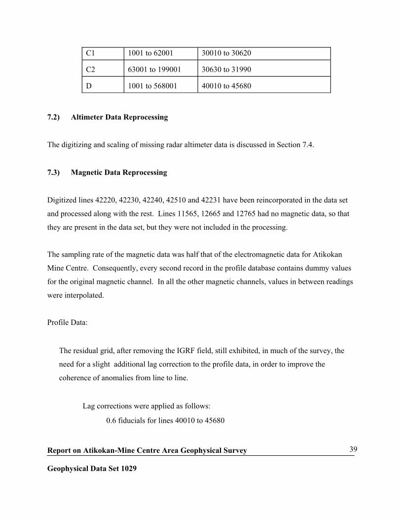
C1 1001 to 62001 30010 to 30620

C2 63001 to 199001 30630 to 31990

D 1001 to 568001 40010 to 45680

7.2) Altimeter Data Reprocessing

The digitizing and scaling of missing radar altimeter data is discussed in Section 7.4.

7.3) Magnetic Data Reprocessing

Digitized lines 42220, 42230, 42240, 42510 and 42231 have been reincorporated in the data set

and processed along with the rest. Lines 11565, 12665 and 12765 had no magnetic data, so that

they are present in the data set, but they were not included in the processing.

The sampling rate of the magnetic data was half that of the electromagnetic data for Atikokan

Mine Centre. Consequently, every second record in the profile database contains dummy values

for the original magnetic channel. In all the other magnetic channels, values in between readings

were interpolated.

Profile Data:

The residual grid, after removing the IGRF field, still exhibited, in much of the survey, the

need for a slight additional lag correction to the profile data, in order to improve the

coherence of anomalies from line to line.

Lag corrections were applied as follows:

0.6 fiducials for lines 40010 to 45680



40



For parts of some lines, the magnetic data appeared mispositioned compared to adjacent lines, so

that a lag correction was applied individually on portions of those lines.

Line 42671: Lag of 24 fiducials from fiducial 1861100 to 1864150

Lag of 38 fiducials from fiducial 1864200 to 1864550

Line 41010: Lag of 14 fiducials from fiducial 260400 to 272350

Line 22860: Lag of 4 fiducials

Line 30800: Lag of 8 fiducials starting from fiducial 384550

Micro-levelling:

For the Atikokan Mine Centre the noise amplitude limit was 80 nT and the Naudy filter

length was 1000 m (see Section 4.3).

Calculation of Reprocessed Total Magnetic Field Grids:

For the Atikokan Mine Centre area three types of total magnetic field grids were generated.

a) Total magnetic field grid (unsmoothed and unfiltered) - AMMAGONL.OMG:

From the total field flight line XYZ data, which was edited, levelled, corrected for

IGRF, micro-levelled, and levelled to the 200m Ontario Single Master Aeromagnetic

grid, a 40m x 40 m cell size grid was computed using the minimum curvature

algorithm. During QC/QA of the total field image, it was noticed that at specific

locations where adjacent flightlines touch or cross each other, minor level differences



41

are apparent. To alleviate this problem and to provide high image quality grids, the

offending section(s) of one of the touching or crossing flightlines, at each location,

was dummied prior to re-gridding and data stored in channel FONLEDTC. The

resultant grid created from this channel is referred to as AMMAGONL.OMG in the

database.

b) Smoothed total magnetic field grid (Hanning filtered) - AMMAGHF.OMG:

High-frequency noise remains in the data after micro-levelling. This noise is not

flightline-related, and likely reflects the vintage of the system used to acquire the

data. To improve the cosmetic appearance of the grid, three passes of a Hanning

smoothing filter were applied to grid AMMAGONL.OMG and a Hanning filtered

grid AMMAGHF.OMG was generated.

c) Bigrid-filtered total magnetic field grid - AMMAGBF.OMG:

After dummying out profiles for touching and/or crossing lines, some effects of

highly irregular flightpath remained present on the total field grid. As an alternative

to the Hanning filter described above, a linear low-pass filter was applied to the grid

AMMAGONL.OMG, perpendicular to the flightline direction of each block. The

filter wavelength was set to

400 m. The resultant Bigrid-filtered grid is AMMAGBF.OMG.

Two channels of magnetic data are provided in the profile database, all of which were

reprocessed, microlevelled and levelled to the Ontario Master Aeromagnetic Grid. They are:



42

Channel FMAGONTL - unsmoothed, no gaps (i.e. no dummy values inserted

where lines touch or cross) and no corresponding grid

was computed

Channel FONLEDTC - unsmoothed, edited to remove sections of crossing or

touching lines and used to prepare the grid

AMMAGONL.OMG.

7.4) Electromagnetic Data Reprocessing

The digital data from lines 11565, 12665 and 12765 of Block A and lines 42220, 42230, 42240,

42510, 42700 and 42231 of Block D, were found to be missing and had to be recovered

(digitized) from the original analogue records.

Recovery of the radar altimeter:

The radar trace on the analogue records was displayed at a vertical scale of 100 feet/cm, with

the value of 400 feet located at the centre of the chart and increasing downward in a linear

fashion. The conversion used, from digitizer units to feet was (value x - 0.255) + 1123.

Recovery of the powerline monitor:

The powerline monitor trace on the analogue records was displayed at a vertical scale of 70

units/cm, increasing downward with a base value of -70. The conversion used from digitizer

units to millivolts (?) was (value x - 0.178) + 976.

Recovery of the INPUT EM channels:



43

The vertical scaling factor of the INPUT channels, as displayed on the analogue records, was

verified by comparing the measured amplitude of channel 2 from selected anomalies, with

the labelled amplitude of channel 2 from the corresponding anomalies, as displayed on the

published anomaly maps. This comparison indicated that the INPUT channels on the

analogue records were displayed at 300 ppm/cm, contrary to the figure of 500 ppm/cm

originally quoted by Questor for this survey. The EM channels were therefore digitized

using a vertical scaling factor of 300 ppm/cm, increasing downward, with a baseline offset of

0.4 cm between each channel. The recovered amplitudes for the affected lines tied-in well

with the data from other lines, supporting the choice of scaling factor used.

Conversion of the EM digital data from millivolts, as stored in the original OGS archives, to

ppm:

The conversion of the EM channel data from millivolts (mV) to ppm is a function of the gain

factors applied to each individual channel at the receiver. The standard gain factors applied

to each channel, as quoted by Questor, were 6.250, 3.125, 1.562, 1.562. 1.562, 1.562 for

channels 1 to 6 respectively.

Again, this was checked by comparing the amplitude in mV of channels for selected

anomalies, with the published amplitudes in ppm for the corresponding responses, as shown

on the EM anomaly maps. It was discovered that the scalar difference between the two sets

of values was approximately 6 to 1 or about twice the quoted factor of 3.125 for channel 2.

Plotting the raw channel amplitude (in mV) from several good conductors, on a log-linear

graph, confirmed that channels 3 to 6 had the same gain, as those plotted along an expected

smooth exponential function. However, channels 1 and 2 did not follow the exponential

curve, indicating that these channels were measured with different gain factors.



44

So,

1) Assuming that the gain used for channel 2 was actually twice the

normal gain of 3.125, we get 6.250.

2) Extrapolating the decay curve from channels 1 and 2 on the log-linear

plot, to follow the exponential curve defined by channels 3 to 6.

3) Establishing the amplitude ratio between channels 1 and 2.

4) Calculating the corresponding channel 1 amplitude in ppm, using

channel (in mV) x 6.25 and the ratio of channel 1 to 2.

We derive a mean gain value for channel 1 of approximately 12 or again about twice the quoted

gain factor of 6.25 for channel 1. It was therefore reasonable to assume that the gain factors for

all channels were set to exactly twice the regular values. The following scalars were therefore

used to convert the data from mV to ppm:

Channel 1 multiplied by 12.5Channel 2 multiplied by 6.25Channel 3 multiplied by 3.125Channel 4 multiplied by 3.125Channel 5 multiplied by 3.125Channel 6 multiplied by 3.125

Lag correction:

All EM data (as recovered from the analogue records and as converted from the digital mV to

ppm) was corrected for 5 samples (2.5 seconds) of system lag. The alignment of EM peaks



45

from vertical conductors (or culture), after the correction, was verified by producing a series

of stacked profile plots.

Base level adjustments:

Difference traces were created for each of the channels, before and after the baseline

levelling adjustments and statistics run on these differences to quantify the adjustments

made.



46

BASE LEVEL ADJUSTMENTS

CHANNEL BLOCK A BLOCK B BLOCK C BLOCK D

1. Mean St. dev.

+ 26 ppm150 ppm

- 78 ppm183 ppm

- 82 ppm123 ppm

- 68 ppm190 ppm

2. Mean St. dev.

- 53 ppm97 ppm

- 34 ppm120 ppm

-103 ppm93 ppm

- 111 ppm211 ppm

3. Mean St. dev.

- 60 ppm92 ppm

- 15 ppm112 ppm

- 141 ppm96 ppm

- 107 ppm134 ppm

4. Mean St. dev.

- 54 ppm96 ppm

- 7 ppm106 ppm

- 107 ppm83 ppm

- 122 ppm106 ppm

5. Mean St. dev.

- 55 ppm116 ppm

- 40 ppm95 ppm

- 202 ppm71 ppm

- 118 ppm105 ppm

6. Mean St. dev.

+ 92 ppm154 ppm

+ 40 ppm90 ppm

+ 67 ppm137 ppm

+ 137 ppm105 ppm

Irregular decays:

Irregular decays in the late channels (4, 5 and 6) over strong conductors were noted. These

events likely reflect deficiencies in the original compensation of the data which was known

to occur with this vintage of the INPUT system, in areas of strong ground response

(essentially the result of an over compensation for the primary field caused by higher

conductive grounds). During the reprocessing, only three things could be addressed: baseline

levels, general noise and singular bad values. In the lines where irregular decays were noted

over strong conductors, the baseline levels in the background resistive regions were

confirmed to be good. This indicates that the irregular decays noted were not due to poor

baseline levels but to localized effects of over compensation which cannot be corrected for.



47

Summary of EM Data Processing Parameters Used:

1. Lag adjustment: 5 samples for EM channels, 5 samples for Hz monitor

2. Base level adjustments: interactively done via a graphic screen

3. Conversion of EM channels Ch 1 x 12.5, Ch 2 x 6.25, Ch 3 to 6 x 3.125from mV to ppm:

4. Editing of spherics: removed by interpolation via a graphic screen

5. EM channel filtering: triangular adaptive filter used, minimum filter width of3 points, maximum filter used of 11 points, localgradient threshold of 15 ppm, followed by a 3 pointrunning average.

6. TAU values: channels 1 to 6 fitted to an exponential function, noisethreshold of 25 ppm

7. Filtering of TAU: 11 point bell filter

8. Resistivity values: translated from the TAU values, channels 1 to 6 used,noise threshold of 25 ppm, homogeneous-half-spacemodel

9. Gridding of EM: 40 m cell size, linear interpolation

10. Anomaly selection: vertical plate model used (600 m strike length by 300 mdepth extent). Channels 1 to 6 used, noise threshold infitting 20 ppm. Minimum amplitude accepted forchannels 1 to 6: 120, 85, 70, 55, 45, 35 ppm.

7.5) Known Data Bugs

The original magnetic data contained a fair degree of high-frequency noise. This noise remains

in the final levelled, but unfiltered, magnetic data. Lines 11565, 12665 and 12765 have no

magnetic data.

REFERENCES

Akima, H., 1970, A new method of interpolation and smooth curve fitting based on localprocedures, Journal of Association for Computing Machinery, v. 17, no. 4, p. 589-602.

Briggs, Ian, 1974, Machine contouring using minimum curvature, Geophysics, v.39, p.39-48.

Dyck, A. V., and Bloore, M., 1980, The response of a rectangular thin plate conductor,Geophysics documented program library, University of Toronto, Research in AppliedGeophysics No. 14.

Gupta, V. and Ramani, N., 1982, Optimum second vertical derivatives in geological mappingand mineral exploration, Geophysics, v.47, p. 1706-1715.

Gupta, V. K., Paterson, N., Reford, S.W., Kwan, K., Hatch, D., and MacLeod, I., 1989, Singlemaster aeromagnetic grid and magnetic color maps for the province of Ontario; inSummary of Field Work and Other Activities 1989, Ontario, Geological Survey,Miscellaneous Paper 146, p. 244-250.

Keating, P.B. 1995. A simple technique to identify magnetic anomalies due to kimberlite pipes;Exploration and Mining Geology, v.4, no.2, p.121-125.

Minty, B.R.S., 1991, Simple micro-levelling for aeromagnetic data, Exploration Geophysics, v.22, p. 591-592.

Naudy, H., Dreyer, H., 1968, Essai de filtrage nonlineaire applique aux profils aeromagnetiques,Geophysical Prospecting, v.16, no.2, p.171.

Reford, S.W., Gupta,V.K., Paterson, N.R., Kwan, K.C.H., and MacLeod, I.N., 1990, The Ontariomaster aeromagnetic grid: a blueprint for detailed compilation of magnetic data on aregional scale, Expanded Abstracts of the Annual Meeting of the Society of ExplorationGeophysicists, p.617-619.

Vaughan, C., 1988, A Novel Approach to AEM Data Compilation, Proceedings of the USGSsponsored AEM Workshop, Denver, Colorado.

Widrow, B., Glover, J.R., McCool, J.M., Kaunitz, J., Williams, C.S., Hearn, R.H., Zeidler, J.R.,Dong, E., Goodlin, R.C. 1975. Adaptive noise cancelling: Principles and Applications,Proceedings of the IEEE, v.63, no.12, p.1692-1716.



49

APPENDIX A

SURVEY HISTORY

A) Introduction: Contractor: Questor Surveys Ltd.Type of Survey: TDEM (INPUT)Size: 15,497kmDates flown: December 12, 1979 to March 24,

1980Flight grid: lines at 200 m spacing.

Direction:Block A, N-S, Block B, N 05�WBlock C1, N80� WBlock C2, N45�WBlock D, N-SOrthogonal control lines

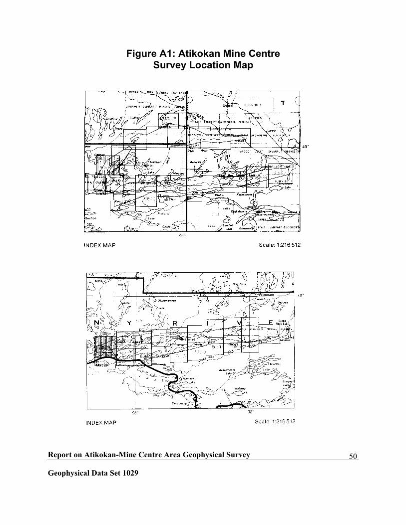
B) Location: Nearest town: Fort FrancesCoordinates: Latitude 48�30' N to 49�10' N Longitude 90o 00' W to 93o 30' WOGS map numbers: 80513 to 80535 inclusive



50

Figure A1: Atikokan Mine CentreSurvey Location Map



51

C) Survey equipment on-board the aircraft:- EM System

Model: INPUT MK VIType: TDEMCoil orientation: horizontalTransmitter loop: 190 m2

Frequency: 144 HzPulse width: 1.05 msOff-time: 2.422 msRx-Tx separation: horizontal 93 m

vertical 69 mSample interval: 0.5 secondIntegration time constant: 1.25 secNumber of channels: 6Channel mid-positions from turn-off: 0.27, 0.45, 0.72, 1.08, 1.53,

2.07 ms

- MagnetometerModel: Sonotek 5010Type: Proton precessionSensitivity: 1 nTSampling interval: 1 secInstallation: Nose boom

- Base stationModel: Geometrics 823Type: Proton precessionSensitivity: 1 nTSampling interval: 10 sec

- Altimeter Sperry radar altimeter

- Analogue recorderHoneywell Visicorder WS 4010

- Digital Acquisition SystemSonotek SDS 1200Digit data 800 bpi 9-track tape drive

- Tracking CameraGeocam 75 F (35 mm) continuous strip



52

- Navigation sytemsDoppler

- AircraftType: Skyvan, model SH-7Average airspeed: 115 knotsMean Terrain clearance: 122 mEM sensor height: 55 mMag sensor height: 122m



53

APPENDIX B

CONTENTS OF PROFILE, GRID, KEATING AND ELECTROMAGNETIC ANOMALY

DATABASES

ATIKOKAN MINE CENTRE Area (AM), Ontario - Profile Database Contents:

The profile data are provided in two formats, one ASCII and one binary:

.csv - flat ASCII file

.gdb - Geosoft OASIS montaj binary database file (no compression)

Both file types contain the same set of data channels, summarized as follows:

LINE Survey/Control line numberTIME seconds TimeX_NAD27 metres UTM Easting NAD27 Zone 15Y_NAD27 metres UTM Northing NAD27 Zone 15X_NAD83 metres UTM Easting NAD83 Zone 15Y_NAD83 metres UTM Northing NAD83 Zone 15FID seconds FiducialLAT_NAD27 degrees Latitude NAD27LON_NAD27 degrees Longitude NAD27LAT_NAD83 degrees Latitude NAD83LON_NAD83 degrees Longitude NAD83FRADAR metres Final Radar AltimeterO60HZMON microvolts Original Hydro MonitorF60HZMON microvolts Final Hydro MonitorOMAGLEV nT Original Magnetic Total FieldFMAGEDIT nT Final Edited Magnetic FieldFMAGIGRF nT Final IGRF FieldFMAGONTL nT Final Total Magnetic Field Levelled to

Ontario Single Master GridFONLEDTC nT Final Total Magnetic Field Levelled to

OntarioSingleMaster Grid –Touching or crossing linesdatadummied

REMCH01 millivolt Raw EM Channel 1REMCH02 millivolt Raw EM Channel 2REMCH03 millivolt Raw EM Channel 3



54

REMCH04 millivolt Raw EM Channel 4REMCH05 millivolt Raw EM Channel 5REMCH06 millivolt Raw EM Channel 6RPEMCH01 ppm Processed EM Channel 1 (this project)RPEMCH02 ppm Processed EM Channel 2 (this project)RPEMCH03 ppm Processed EM Channel 3 (this project)RPEMCH04 ppm Processed EM Channel 4 (this project)RPEMCH05 ppm Processed EM Channel 5 (this project)RPEMCH06 ppm Processed EM Channel 6 (this project)FEMCH01 ppm Final EM Channel 1FEMCH02 ppm Final EM Channel 2FEMCH03 ppm Final EM Channel 3FEMCH04 ppm Final EM Channel 4FEMCH05 ppm Final EM Channel 5FEMCH06 ppm Final EM Channel 6DECAYCON microseconds Apparent Decay ConstantCONDTVTY S/m Apparent Halfspace ConductivityRESIST ohm-m Apparent Halfspace Resistivity

Grids:

The gridded data are provided in two formats, one ASCII and one binary:

*.gxf - ASCII Grid eXchange Format (revision 3.0)

*.grd - Geosoft OASIS montaj binary grid file (no compression)

*.gi - binary file that defines the coordinate system for the *.grd file

Grids are named so that the first two characters are the survey area initials followed by a

standard set of grid type codes, e.g., AMDCDE is the Decay Constant De-herringboned for

ATIKOKAN MINE CENTRE Area (AM).

dc microseconds Decay Constantdcde microseconds Decay Constant Deherringboneddcdef microseconds Decay Constant Deherringboned and Filteredres ohm-m Resistivityresde ohm-m Resisitivity Deherringbonedresdef ohm-m Resisitivity Deherringboned and Filteredmagonl nT Total Magnetic Field levelled to Ontario Single

Master Grid



55

magbf nT Bi-directional low pass filtered Total MagneticField grid

maghf nT Hanning filtered Total Magnetic Field gridmag2vd nT/m2 Second vertical derivative of the Total MagneticField2vdbf nT/m2 Bi-directional low pass filtered second vertical

derivative grid2vdhf nT/m2 Hanning filtered second vertical derivative grid

Time domain Anomaly Database Contents:

The electromagnetic anomaly data are provided in two formats, one ASCII and one binary:.csv – ASCII comma-delimited format.gdb – Geosoft OASIS montaj binary database file


ID na Unique Anomaly identifier (see Note 3)Data_id na Dataset identifierFlight na Flight numberLine na Line numberLet na Numeric Anomaly identifier for Line (see Note 4)Fid na Fiducial value at anomaly peakLON_NAD27 Dec. degrees Longitude NAD27LAT_NAD27 Dec. degrees Latitude NAD27LON_NAD83 Dec. degrees Longitude NAD83LAT_NAD83 Dec. degrees Latitude NAD83Cat N,S,C,Q Anomaly type (N=normal, S=surficial,C=cultural,

Q=Undetermined)Alt m Aircraft terrain clearanceTau microseconds Apparent decay constantRes ohm-m Apparent resistivity from half-space modelP_CH ppm Amplitude of initial picking channel (Channel 03)L_CH ppm Amplitude of later reference channel (Channel 05)NC na Number of channels deflected above backgroundnoiseCTP S Derived conductivity-thickness-productDEP m Derived depth below surface to top of the sourceLine_part na Line part number (Used to identify reflown lines)Line_type na Line type (L=survey line T=tie line)Azim degree E of N Average line heading



56

X_NAD27 m UTM Easting NAD27 Zone 15Y_NAD27 m UTM Northing NAD27 Zone 15X_NAD83 m UTM Easting NAD83 Zone 15Y_NAD83 m UTM Northing NAD83 Zone 15

SYSTEM CONFIGURATION: Pulse repetition rate.......................................144 Hz Pulse width....................................................1050 us Offtime..........................................................2422 us Receiver-transmitter horizontal separation.........93 m Receiver-transmitter vertical separation..............69 m Receiver axis orientation............................Horizontal

MODEL USED IN FITTING: Vertical plate model Length of 600 m Depth extent of 300 m Vertical dip Strike perpendicular to flight line

NOTE 1. Selections with 0 in the CTP and DEP columns reflect surficial or cultural selections,

which were not fitted to the vertical plate model.

NOTE 2. Selections with a negative number shown in the DEP column indicate a normal

selection (bedrock) where the vertical plate model used does not properly reflect the true

conductor geometry.

NOTE 3. For non-cultural anomalies, the unique anomaly identifier is a ten digit integer in the

format 1LLLLLLAAA where 'LLLLLL' holds the line number (and leading zeroes pad short line

numbers to six digits). The 'AAA' represents the numeric anomaly identifier for that line padded

with leading zeroes to three digits. For cultural anomalies, the leading numeral '1' and any line

number padding zeroes are omitted so that cultural anomalies have a four to nine digit integer.

For example, 1000101007 represents the seventh non-cultural anomaly on Line 101, 101005

represents the fifth cultural anomaly on Line 101, and 590101002 represents the second cultural

anomaly on Line 590101.



57

NOTE 4. Numeric anomaly identifiers count up independently for cultural and non-cultural

classifications.

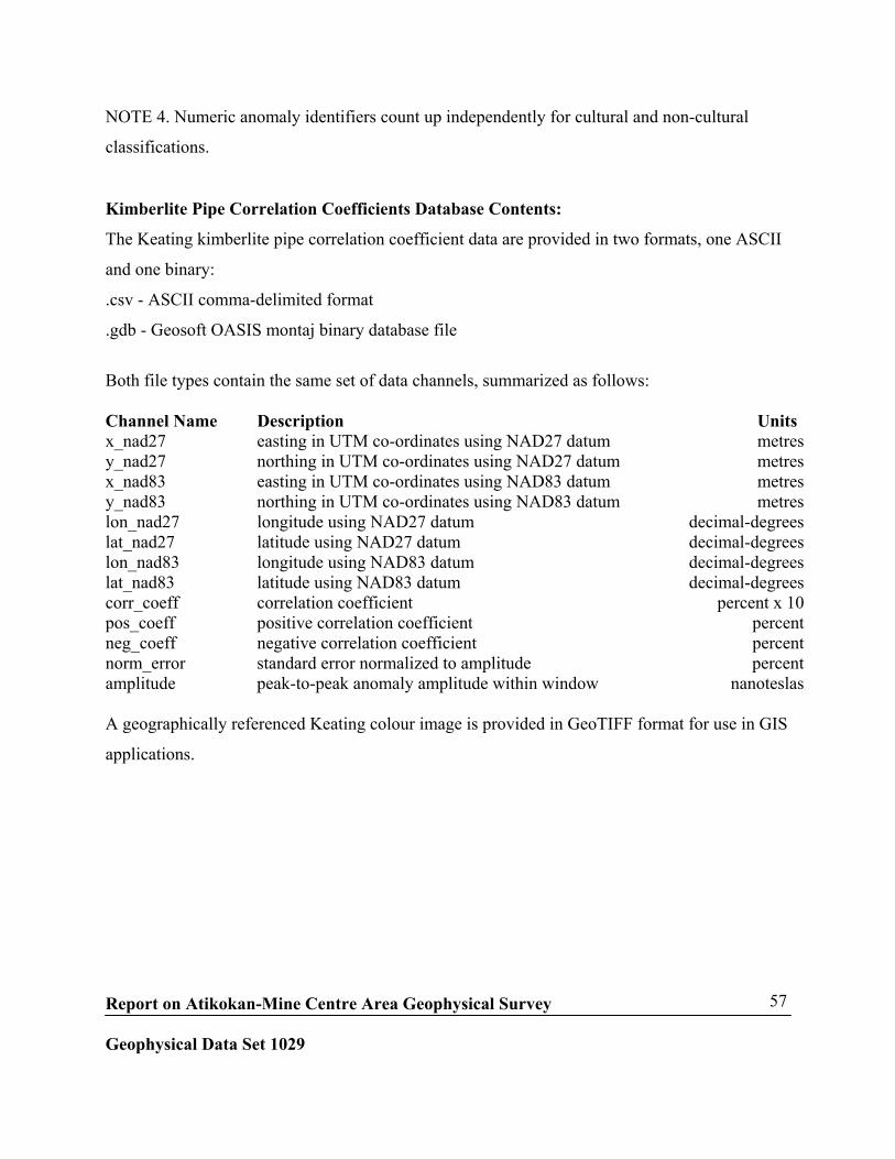
Kimberlite Pipe Correlation Coefficients Database Contents:

The Keating kimberlite pipe correlation coefficient data are provided in two formats, one ASCII

and one binary:

.csv - ASCII comma-delimited format

.gdb - Geosoft OASIS montaj binary database file


Channel Name Description Unitsx_nad27 easting in UTM co-ordinates using NAD27 datum metresy_nad27 northing in UTM co-ordinates using NAD27 datum metresx_nad83 easting in UTM co-ordinates using NAD83 datum metresy_nad83 northing in UTM co-ordinates using NAD83 datum metreslon_nad27 longitude using NAD27 datum decimal-degreeslat_nad27 latitude using NAD27 datum decimal-degreeslon_nad83 longitude using NAD83 datum decimal-degreeslat_nad83 latitude using NAD83 datum decimal-degreescorr_coeff correlation coefficient percent x 10pos_coeff positive correlation coefficient percentneg_coeff negative correlation coefficient percentnorm_error standard error normalized to amplitude percentamplitude peak-to-peak anomaly amplitude within window nanoteslas

A geographically referenced Keating colour image is provided in GeoTIFF format for use in GIS

applications.



58

APPENDIX C

2002 DIGITAL ARCHIVE RE-FORMATTING NOTES

The changes made to the AMEM digital archives during the 2002 data re-formatting project are

described below.

Coordinate Systems

The data are provided in four coordinate systems:

Universal Transverse Mercator (UTM) projection, Zone 15N, NAD27 datum (NTv2) local

datum;

Universal Transverse Mercator (UTM) projection, Zone 15N, NAD83 datum, North American

local datum;

Latitude/longitude coordinates, NAD27 datum (NTv2) local datum; and

Latitude/longitude coordinates, NAD83 datum, North American local datum.

The gridded data are provided in the two Zone 15 UTM coordinate systems (NAD27_NTv2 and

NAD83) as indicated by the codes “27” or “83” affixed to the file name.

ATIKOKAN MINE CENTRE Ontario Airborne Magnetic and

Documents

Transcript of ATIKOKAN MINE CENTRE Ontario Airborne Magnetic and