ATHENS UNIVERSITY OF ECONOMICS AND BUSINESS · 2 Professor of Economics, Athens University of...
54
ATHENS UNIVERSITY OF ECONOMICS AND BUSINESS WORKING PAPER SERIES 05‐2013 Quantitative price tests in antitrust market definition with an application to the savory snacks markets Yannis Katsoulacos, Ioanna Konstantakopoulou, Eleni Metsiou & Efthymios G. Tsionas 76 Patission Str., Athens 104 34, Greece Tel. (++30) 210‐8203911 ‐ Fax: (++30) 210‐8203301 www.econ.aueb.gr
Transcript of ATHENS UNIVERSITY OF ECONOMICS AND BUSINESS · 2 Professor of Economics, Athens University of...
ATHENS UNIVERSITY OF ECONOMICS AND BUSINESS
WORKING PAPER SERIES 05‐2013
Quantitative price tests in antitrust market definition with an application to the savory snacks markets
Yannis Katsoulacos, Ioanna Konstantakopoulou, Eleni Metsiou &
Efthymios G. Tsionas
76 Patission Str., Athens 104 34, Greece
Tel. (++30) 210‐8203911 ‐ Fax: (++30) 210‐8203301
www.econ.aueb.gr
1
Quantitative price tests in antitrust market definition with an application to the savory
snacks markets1
Yannis Katsoulacos2, Ioanna Konstantakopoulou3, Eleni Metsiou4 & Efthymios G. Tsionas5
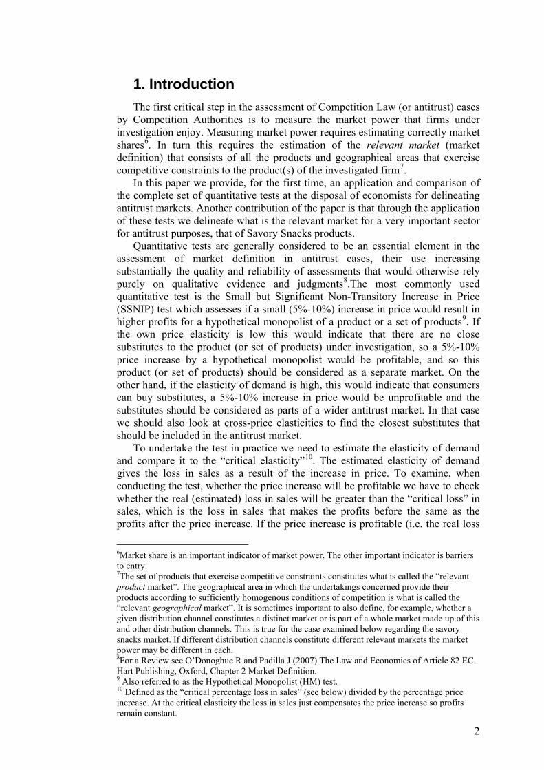
ABSTRACT
In this paper we utilize for the first time and compare by applying in succession the complete set of quantitative tests for delineating antitrust markets. This includes the Small but Significant Increase in Price (SSNIP) test but also a large number of traditional and newer price co-movement tests. We apply these tests to the Savory Snacks Market using Greek bi-monthly data. This market has been subject to many antitrust investigations because of its important implications for welfare and its market structure. However, no dominant view has yet emerged regarding the appropriate definition of the relevant market. Our results indicate that a wide relevant market definition is appropriate.
Keywords: market definition, quantitative price-comovement tests, savory snacks market.
JEL Code: K21, L40, L66
1 We are grateful for the comments of the participants of the 7th Annual CRESSE Conference (Chania, 6-8 July, 2012), on “Advances in the Analysis of Competition Policy and Regulation”, in which a previous version of this paper was presented. We would like to thank particularly, Frank Verboven, Marc Ivaldi, Willem Boshoff and Veit Böckers. Of course, all errors and ambiguities remain our responsibility. This research has been co-financed by the European Union (European Social Fund – ESF) and Greek national funds through the Operational Program "Education and Lifelong Learning" of the National Strategic Reference Framework (NSRF) - Research Funding Program: Thalis – Athens University of Economics and Business - Thalis – Athens University of Economics and Business - NEW METHODS IN THE ANALYSIS OF MARKET COMPETITION: OLIGOPOLY, NETWORKS AND REGULATION. 2 Professor of Economics, Athens University of Economics and Business, Address: Patission 76, 104 34, Athens, GREECE, Tel: +30 210 8203348, Fax: +30 2108223259, e-mail: [email protected], [email protected], http://www.aueb.gr/users/katsoulacos/ 3 Researcher, Center of Planning and Economic Research (KEPE). 4 PhD Candidate, Athens University of Economics and Business. 5 Professor of Economics, Athens University of Economics and Business.
2
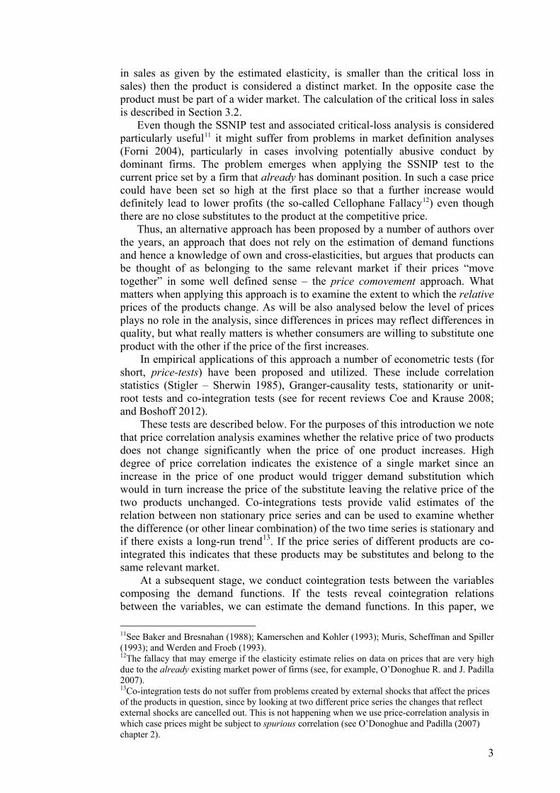
1. Introduction The first critical step in the assessment of Competition Law (or antitrust) cases
by Competition Authorities is to measure the market power that firms under investigation enjoy. Measuring market power requires estimating correctly market shares6. In turn this requires the estimation of the relevant market (market definition) that consists of all the products and geographical areas that exercise competitive constraints to the product(s) of the investigated firm7.
In this paper we provide, for the first time, an application and comparison of the complete set of quantitative tests at the disposal of economists for delineating antitrust markets. Another contribution of the paper is that through the application of these tests we delineate what is the relevant market for a very important sector for antitrust purposes, that of Savory Snacks products.
Quantitative tests are generally considered to be an essential element in the assessment of market definition in antitrust cases, their use increasing substantially the quality and reliability of assessments that would otherwise rely purely on qualitative evidence and judgments8.The most commonly used quantitative test is the Small but Significant Non-Transitory Increase in Price (SSNIP) test which assesses if a small (5%-10%) increase in price would result in higher profits for a hypothetical monopolist of a product or a set of products9. If the own price elasticity is low this would indicate that there are no close substitutes to the product (or set of products) under investigation, so a 5%-10% price increase by a hypothetical monopolist would be profitable, and so this product (or set of products) should be considered as a separate market. On the other hand, if the elasticity of demand is high, this would indicate that consumers can buy substitutes, a 5%-10% increase in price would be unprofitable and the substitutes should be considered as parts of a wider antitrust market. In that case we should also look at cross-price elasticities to find the closest substitutes that should be included in the antitrust market.
To undertake the test in practice we need to estimate the elasticity of demand and compare it to the “critical elasticity”10. The estimated elasticity of demand gives the loss in sales as a result of the increase in price. To examine, when conducting the test, whether the price increase will be profitable we have to check whether the real (estimated) loss in sales will be greater than the “critical loss” in sales, which is the loss in sales that makes the profits before the same as the profits after the price increase. If the price increase is profitable (i.e. the real loss
6Market share is an important indicator of market power. The other important indicator is barriers to entry. 7The set of products that exercise competitive constraints constitutes what is called the “relevant product market”. The geographical area in which the undertakings concerned provide their products according to sufficiently homogenous conditions of competition is what is called the “relevant geographical market”. It is sometimes important to also define, for example, whether a given distribution channel constitutes a distinct market or is part of a whole market made up of this and other distribution channels. This is true for the case examined below regarding the savory snacks market. If different distribution channels constitute different relevant markets the market power may be different in each. 8For a Review see O’Donoghue R and Padilla J (2007) The Law and Economics of Article 82 EC. Hart Publishing, Oxford, Chapter 2 Market Definition. 9 Also referred to as the Hypothetical Monopolist (HM) test. 10 Defined as the “critical percentage loss in sales” (see below) divided by the percentage price increase. At the critical elasticity the loss in sales just compensates the price increase so profits remain constant.
3
in sales as given by the estimated elasticity, is smaller than the critical loss in sales) then the product is considered a distinct market. In the opposite case the product must be part of a wider market. The calculation of the critical loss in sales is described in Section 3.2.
Even though the SSNIP test and associated critical-loss analysis is considered particularly useful11 it might suffer from problems in market definition analyses (Forni 2004), particularly in cases involving potentially abusive conduct by dominant firms. The problem emerges when applying the SSNIP test to the current price set by a firm that already has dominant position. In such a case price could have been set so high at the first place so that a further increase would definitely lead to lower profits (the so-called Cellophane Fallacy12) even though there are no close substitutes to the product at the competitive price.
Thus, an alternative approach has been proposed by a number of authors over the years, an approach that does not rely on the estimation of demand functions and hence a knowledge of own and cross-elasticities, but argues that products can be thought of as belonging to the same relevant market if their prices “move together” in some well defined sense – the price comovement approach. What matters when applying this approach is to examine the extent to which the relative prices of the products change. As will be also analysed below the level of prices plays no role in the analysis, since differences in prices may reflect differences in quality, but what really matters is whether consumers are willing to substitute one product with the other if the price of the first increases.
In empirical applications of this approach a number of econometric tests (for short, price-tests) have been proposed and utilized. These include correlation statistics (Stigler – Sherwin 1985), Granger-causality tests, stationarity or unit-root tests and co-integration tests (see for recent reviews Coe and Krause 2008; and Boshoff 2012).
These tests are described below. For the purposes of this introduction we note that price correlation analysis examines whether the relative price of two products does not change significantly when the price of one product increases. High degree of price correlation indicates the existence of a single market since an increase in the price of one product would trigger demand substitution which would in turn increase the price of the substitute leaving the relative price of the two products unchanged. Co-integrations tests provide valid estimates of the relation between non stationary price series and can be used to examine whether the difference (or other linear combination) of the two time series is stationary and if there exists a long-run trend13. If the price series of different products are co-integrated this indicates that these products may be substitutes and belong to the same relevant market.
At a subsequent stage, we conduct cointegration tests between the variables composing the demand functions. If the tests reveal cointegration relations between the variables, we can estimate the demand functions. In this paper, we
11See Baker and Bresnahan (1988); Kamerschen and Kohler (1993); Muris, Scheffman and Spiller (1993); and Werden and Froeb (1993). 12The fallacy that may emerge if the elasticity estimate relies on data on prices that are very high due to the already existing market power of firms (see, for example, O’Donoghue R. and J. Padilla 2007). 13Co-integration tests do not suffer from problems created by external shocks that affect the prices of the products in question, since by looking at two different price series the changes that reflect external shocks are cancelled out. This is not happening when we use price-correlation analysis in which case prices might be subject to spurious correlation (see O’Donoghue and Padilla (2007) chapter 2).
4
estimate demand elasticities using the FMOLS estimation technique for heterogeneous cointegrated panels (Pedroni 2000).
The need for the use of price tests has been stressed most forcefully by Forni (2004) who argued that price co-movement tests are the only satisfactory tests in dominance cases and generally can provide very reliable results. Nevertheless price co-movement tests have been criticized too (e.g. Bishop and Walker 2002)14, though to some extent the more recent criticisms may be due to inadequate understanding of the latest improvements in econometric theory and techniques (e.g. in relation to estimation using small samples).
In our current study we apply the SSNIP as well as price correlation, Granger Causality and unit root and cointegration tests to the Savory Snacks Market using Greek bi-monthly data. Our research was triggered by the recent TASTY (a subsidiary of PepsiCo) case of the Hellenic Competition Commission, further analysed in section 2.1, for infringements of Art. 102 TFEU15 regarding potential abuse of dominant position. Because of its important implications for consumer welfare and its market structure, the Savory Snacks market is one of the most interesting markets from the point of view of Competition Policy enforcement worldwide. Anticompetitive practices or mergers, that could result in price increases, are likely to have a significant adverse impact on consumer welfare as this is a very large market and its segments, especially chips and nuts & seeds, constitute important parts of the daily diets of significant consumer groups (such as the younger age groups)16. The market’s global value in 2009 was 68 billion USD, growing at an average yearly rate of 5,1% between 2004 and 2009. The market is forecast to have a value of 87 billion USD in 201417. It is also a market characterized by high levels of concentration in most countries, with just one US multinational (PepsiCo) controlling almost 30% of the total world market18, as well as high levels of product differentiation. Given these facts, it is no wonder that the market has been subject to a very large number of antitrust investigations worldwide and, given the market’s structure, this trend is most likely to continue.
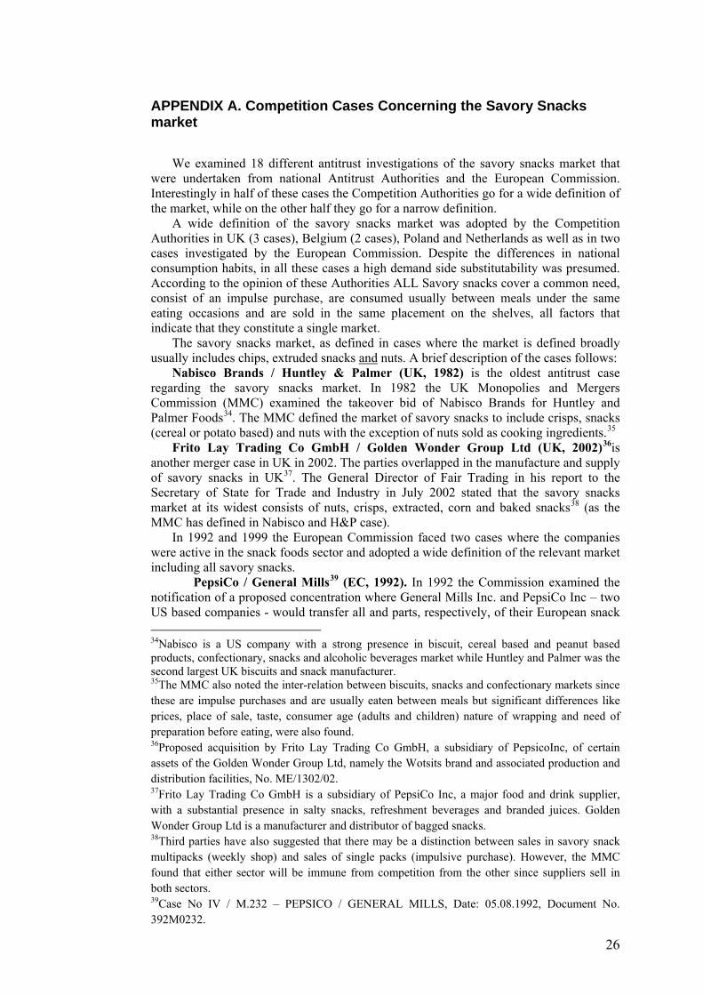
We identified 18 different antitrust investigations of this market, presented in Appendix A., in the last 20 years or so. What is most interesting is that despite the very large number of investigations there is still no dominant view regarding the appropriate definition of the relevant market: in half of the investigations, the competition authorities go for a wide definition of the market and in the other half they go for a narrow definition!
In our study of the Savory Snacks market in Greece we faced most of the typical problems of obtaining reliable demand elasticity estimates OR estimates that could permit us to identify the relevant markets by using the SSNIP test. The potential problems are:
a) Insufficient data. b) Contrary to intuition and perhaps even contrary to qualitative marketing
information, demand estimation can result in cross-elasticities with the wrong sign or that are statistically insignificant. As Hausman and Leonard
14Thus it has been pointed out that price-tests are subject to spurious correlation and can, at best, define an “economic market” and not an “antitrust market”. See Coe and Krause, 2008 and Boshoff, 2012. The latter argues that this is not a valid criticism. 15This is the European Union Competition (or antitrust) Law that regulates the behavior of dominant firms (or firms with significant market power). 16The market is usually thought of as composed of the following product segments: chips, nuts and seeds, processed snacks, other savory snacks and popcorn. 17Source: Datamonitor Research Store. 18Source: Datamonitor Research Store.
5
(2005) have pointed out “this is not unusual” (page 293) and in the empirical example that they provide (for the market of health and beauty aid) using AIDS (Almost Ideal Demand System), they do indeed get a number of statistically insignificant cross-elasticities.
c) Own price elasticity estimates may lack credibility due to the Cellophane Fallacy.
For this reason, in our analysis, we complemented the SSNIP test and traditional qualitative analysis with a battery of other quantitative tests including price correlation, Granger causality and other (unit root and cointegration) price-tests looking at both short-run and long-run relationships and then tried to delineate markets on the basis of the results obtained from all these tests19. We would argue as our methodological proposition that, if it is the case that all these tests point in the same direction then this provides a strong prima facie reason to think that this direction is the right one.
The Savory Snacks market is usually thought of as consisting of Salty Snacks and Sweet Snacks. Savoury Salty Snacks is made up of three main segments:
- The Core Salty Snack (CSS) segment (consisting of salty potato-based snacks, mainly chips, and salty snacks based on potato derivatives).
- The Nuts segment. - The Other Salty Snacks segment consisting of salty flour-based snacks
(such as salty biscuits, bake rolls, bake bars, crackers etc.). A strong position in the CSS section, as in the case of PepsiCo (TASTY) in
Greece where the company has had a high market share of about 75% in this segment, would be characterized as a position of dominance or even super-dominance, if it is decided that CCS constitutes a distinct relevant market. However, even the inclusion of one of the other segments/categories of Salty Snacks would often lower market share to below 50%, and if all three segments were included the market share could fall to something close to 30%. Of course, market shares would usually be below 20% if Salty and Sweet Savory Snacks were categorized in the same relevant market.
The paper is organized as follows: in Section 2 we describe the Greek Savory Snacks market that has been the subject of our investigation and provide some details of the case, for Abuse of Dominant position by PepsiCo, examined in 2010-12 by the Hellenic Competition Commission. In Section 3 we describe the approach we followed in assessing the extent of the relevant market, the data used, the problems we faced and the tests we performed as well as the results of these tests. In Section 4 we conclude.
2. Brief Description of the Greek Savory Snacks Market and Qualitative Evidence on Market Definition 2.1. Introduction and background to the case
In 2007 TASTY FOODS (a subsidiary of the PepsiCo Inc Group) was accused by TSAKIRIS (which belongs to the Coca Cola 3E Group) of infringements of Articles 1 and 2 of the Greek Competition Law 703/77 and of 19We should stress that we certainly do not disagree with those economists arguing that the SSNIP test is the most appropriate test in market delineation cases. However, at the same time, we do not think that one should abandon all attempts to delineate relevant markets when the SSNIP cannot guarantee credible results.
6
Articles 101 and 102 TFEU of EU Competition Law in connection with commercial practices employed. By its Decision No. 520/VI/2011, the Hellenic Competition Commission found that TASTY FOODS, infringed Articles 2 of Greek Law 703/77 and 102 TFEU (abuse of dominance) and fines of €16.177.514 million were imposed on the company.
To assess the dominance of TASTY in the relevant market, and by extension the possible abuse of it, the Hellenic Competition Commission decided that the relevant market should include only chips and potato derivatives. In other words it was decided that the Core Salty Sector constitutes a distinct relevant market. The Hellenic Competition Commission further stated that the market can also be segmented according to the distribution channels to the Organised Trade channel (OT), that includes Super Markets, and the Small Drop Outlets (SDOs) or Down-The-Street (DTS) channel, that includes kiosks, mini markets, bakeries and special channels.
As noted above, TASTY has a high market share in the Core Salty Sector exceeding 70%. However, even the inclusion of one of the other segments/categories of Salty Snacks would lower market share to below 50%. This is indicative of the high importance of the right definition of the relevant market since market share is one of the main indicators used by Competition Authorities in order to determine if a firm’s position is dominant.
In our investigation of the right boundaries we examined whether Core Salty Snacks (chips, extruded, corn chips) and Nuts constitute distinct markets or if alternatively these sectors are parts of a wider market that includes both. We also examine whether distribution channels are distinct markets since, if this is so, it is more likely that there will be market power in at least one channel (see also below).
In this section, we first describe the qualitative evidence regarding the substitution between different salty snacks and then we examine the possibility that the two different distribution channels (OT and DTS) are distinct relevant markets.
2.2 Qualitative evidence
According to the EC’s Guidance20 for the definition of the Relevant Markets, qualitative factors that affect the demand substitution should also be taken into account and analysed. These factors include switching costs, natural characteristic of the products, intended use and differences in price.
However, it should be noted that these factors should be strictly examined within the framework of substitution effects, and not merely as factors that can define per se the relevant market. For example price differences can be high as a result of different costs but this does not mean that an increase of 5-10% in the relative price of a product will not lead to a higher percentage demand switch to another product.
First of all, it is apparent that in the case of the savory snacks market there are no transaction or learning switching costs. The Statement of Objections21 made a vague reference regarding the differences in natural characteristics of the products, the natural ingredients, to exclude dry nuts from the relevant market. 20 Commission Notice on the definition of relevant market for the purposes of Community Competition Law (97/C 372/03), 09.12.97 available in http://europa.eu/legislation_summaries/competition/firms/l26073_en.htm. 21The Statement of Objections is the Report that has to be prepared by the Competition Commission explaining why it considers a firm’s action as anticompetitive.
7
However, even though natural ingredients is an important index for the degree of substitution between two products the information has to be used strictly within the framework of the SSNIP test - reference to product characteristics per se does not suffice for the purpose of defining the market. What really matters is whether consumers view these products as close substitutes and if the switch of the consumers from the one product to the other restricts the possibility of a price increase.
Another reason that the Hellenic Competition Commission invoked to exclude dry nuts from the relevant market was the high difference in prices. However, as it was clearly noted in the example above, absolute price discrepancy does not provide credible information of how demand will be affected by a price increase. Further, substantially different price levels are realized even among salty snacks which belong to the same relevant market according to the Hellenic Competition Commission definition i.e. chips, extruded snacks and corn snacks. Moreover, all salty snacks are considered as substitutable from the consumers’ point of view with regard to the need that these products cover together with the time and motive of consumption. Regarding the intended use of the products at least some studies show that Salty Snacks sector should be considered as the relevant market.
For example the study by Salvetti & Llombart22 in Greece during 2004 found that salty snacks and dry nuts are substitutable and interchangeable from the consumers’ point of view since the time, the place, the nature and the motive of consumption match. Specifically Salvetti and Llombart research found that both salty snacks as well as nuts are usually consumed under the same conditions, for “chilling out” and “socialising”, usually in the afternoon, at home, together with friends while watching TV films or sports in order to fulfill hunger or “nibble”. Euromonitor and European Snack Association23 reach similar conclusions and define an even broader relevant market that includes all salty snacks. Finally, the high degree of substitutability between Core Salty snacks and Nuts is also confirmed by the Research of “Kantar World Panel” with title “Core Salty & Nuts Interaction” in 2009. The research has led to two basic results. First, an inverse influence to the volumes of the two products was observed. If the volume of Core Salty Snacks was decreasing the volume of Nuts would increase and vice versa. Second, the higher shifts in volume of the savory snacks can be observed in the nuts sector. Another indication that all salty snacks belong to the same market is that chips, extruded, corn snacks, dry nuts, bake rolls, bake bars and salty biscuits in Greece are placed on the same Super Market Shelves (OT channel).
2.3 Distribution Channels (OT & DTS)
The Hellenic Competition Commission (for short, Commission) also examined whether the relevant product market may be distinct according to the distribution channel, specifically organized trade (OT) and down-the-street (DTS) channels. The importance of this distinction is that a finding that channels are distinct markets may increase the likelihood that there is significant market power in at least one market (since companies’ market shares will generally not be the same across channels). The Commission stated that these channels may constitute
22Salvetti & Llombart research for the delineation of the Savory Snacks market in Greece (December 2004). 23International databases EUROMONITOR (www.euromonitor.com) and European Snack Association (www.esa.org).
8
different product markets by just noting that the market share of TASTY and its main competitor vary between the channels. However, the variation in market shares does not suffice for the distinction of separate markets. In particular, this difference in market shares should be expected even if the markets are not distinct if TASTY’s efficiency relative to that of its competitors is higher in one of the channels24. Confirming the above, the recent decision of the British Office of Fair Trading, (Walkers Snacks Limited, OFT Decision on 3.5.2007) considering whether there might be separate relevant markets identified with respect to different supply channels (mainly grocery and «impulse» channels) decided to proceed on the basis that the relevant market was likely to comprise both channels.
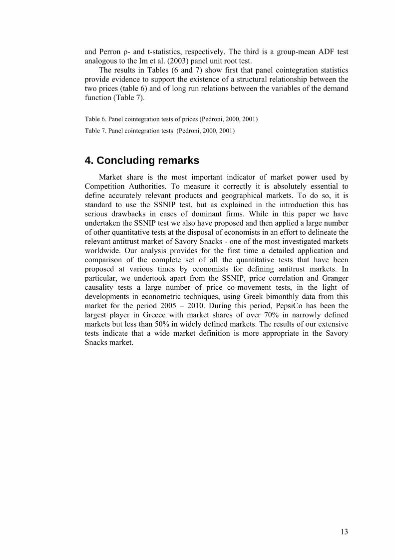
2.4 Market Shares under alternative market definitions
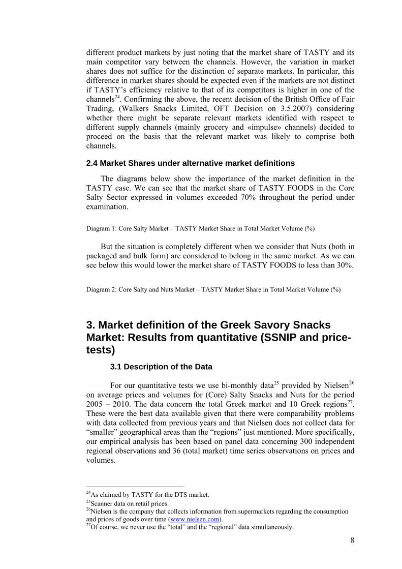
The diagrams below show the importance of the market definition in the TASTY case. We can see that the market share of TASTY FOODS in the Core Salty Sector expressed in volumes exceeded 70% throughout the period under examination.
Diagram 1: Core Salty Market – TASTY Market Share in Total Market Volume (%)
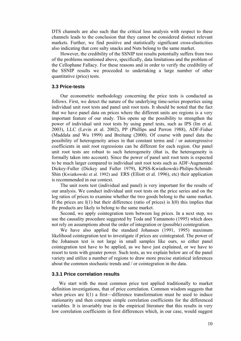
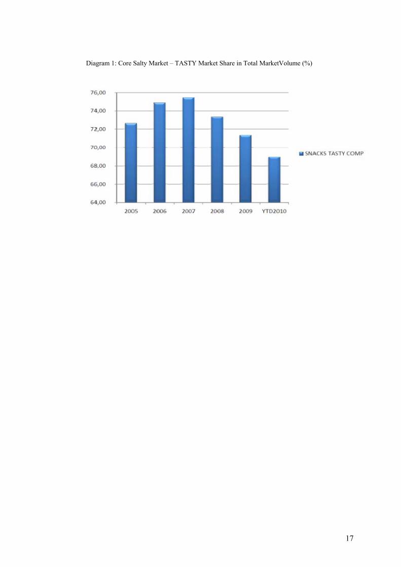
But the situation is completely different when we consider that Nuts (both in
packaged and bulk form) are considered to belong in the same market. As we can see below this would lower the market share of TASTY FOODS to less than 30%.
Diagram 2: Core Salty and Nuts Market – TASTY Market Share in Total Market Volume (%)
3. Market definition of the Greek Savory Snacks Market: Results from quantitative (SSNIP and price-tests)
3.1 Description of the Data For our quantitative tests we use bi-monthly data25 provided by Nielsen26
on average prices and volumes for (Core) Salty Snacks and Nuts for the period 2005 – 2010. The data concern the total Greek market and 10 Greek regions27. These were the best data available given that there were comparability problems with data collected from previous years and that Nielsen does not collect data for “smaller” geographical areas than the “regions” just mentioned. More specifically, our empirical analysis has been based on panel data concerning 300 independent regional observations and 36 (total market) time series observations on prices and volumes.
24As claimed by TASTY for the DTS market. 25Scanner data on retail prices. 26Nielsen is the company that collects information from supermarkets regarding the consumption and prices of goods over time (www.nielsen.com). 27Of course, we never use the “total” and the “regional” data simultaneously.

9
3.2 Demand estimation and the SSNIP test
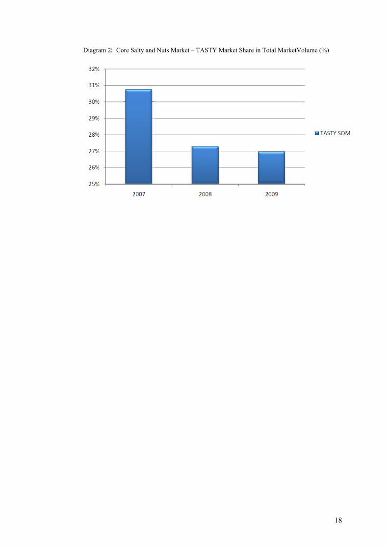
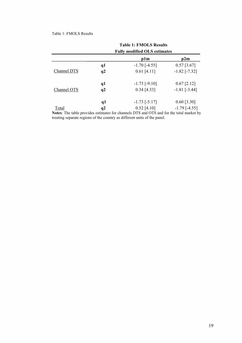
In order to estimate the price elasticities of demand function, we use the Fully Modified OLS (FMOLS) estimator. This estimator developed by Pedroni (2000) does not have the drawbacks of the standard panel OLS estimator (see also section 3.3.4 below). These drawbacks are associated with the fact that a standard panel OLS estimator is asymptotically biased and its standardized distribution is dependent on nuisance parameters associated with the dynamics underlying the data generating processes of variables. To eliminate the problem of bias due to the endogeneity of the regressors, Pedroni suggested the group-means FMOLS estimator, by incorporating the Phillips and Hansen (1990) semi-parametric correction into the OLS estimator. The results of applying the FMOLS procedure in estimating demand functions are shown in the Table 1 below. Concerning the functional form of the demand functions we assume, after imposing zero homogeneity, that this is:
mpmpq 221101 βββ ++= (1) mpmpq 221102 ααα ++= (2)
where: )log( 11 Qq = , )log( 22 Qq = , )/log( 11 Μ= Pmp , )/log( 22 Μ= Pmp ,
1Q and 2Q are quantities, 1P and 2P are prices and 2211 QPQPM += is income (total expenditure). Table 1: FMOLS Results
Critical loss analysis and conclusions from the SSNIP test
Having estimated elasticities, to find the critical loss associated with a given price increase let us denote by m = [(p – c)/c] the percentage margin of a hypothetical monopolist where c is the unit variable cost and p the original (pre-increase) price level and assume that the price increases by a percentage τ (between 5%-10%) reducing output sales by π. The critical loss denoted by π*, is then given by π* = τ/(τ+m)28 and the critical elasticity is ε* = π*/τ. We can see that critical loss and critical elasticity depend on the variable cost of the firm (c). According to the SSNIP test, as described in the introduction, the Core Salty Sector does not constitute a distinct product market if the critical elasticity is less than the elasticity estimate (obtained from the demand estimation). Given a statistically significant elasticity estimate of –1,73 that we found above, the critical loss analysis based on information of the unit variable cost of TASTY29, indicates that certainly the segment of Core Salty Snacks products cannot be considered a distinct relevant product market30. This is because the critical elasticity is below our elasticity estimate31. Our elasticity estimates of the OT and
28So is the percentage loss in sales for which profit after the price increase is equal to profit before the price increase. 29 The results mentioned here hold for price increases between 5% and 10% and for a range of values of the unit variable cost (i.e. they are robust to standard sensitivity analysis). See also O’Donoghue R. and J. Padilla (2007), for further information on the critical loss analysis and the Cellophane Fallacy. 30We assume that the relevant geographic market is the Greek market - the assumption that is always made in investigations of the savory snacks market. We considered this to be a reasonable assumption in view of the very high supply side substitutability between different regions in Greece. 31For reasons of confidentiality (regarding the value of m) we cannot report the value of the critical elasticity.
10
DTS channels are also such that the critical loss analysis with respect to these channels leads to the conclusion that they cannot be considered distinct relevant markets. Further, we find positive and statistically significant cross-elasticities also indicating that core salty snacks and Nuts belong to the same market.
However, the credibility of the SSNIP test results potentially suffers from two of the problems mentioned above, specifically, data limitations and the problem of the Cellophane Fallacy. For these reasons and in order to verify the credibility of the SSNIP results we proceeded to undertaking a large number of other quantitative (price) tests.
3.3 Price-tests
Our econometric methodology concerning the price tests is conducted as follows. First, we detect the nature of the underlying time-series properties using individual unit root tests and panel unit root tests. It should be noted that the fact that we have panel data on prices where the different units are regions is a very important feature of our study. This opens up the possibility to strengthen the power of individual unit root tests by using panel tests, such as IPS (Im et al. 2003), LLC (Levin et al. 2002), PP (Phillips and Perron 1988), ADF-Fisher (Maddala and Wu 1999) and Breitung (2000). Of course with panel data the possibility of heterogeneity arises in that constant terms and / or autoregressive coefficients in unit root regressions can be different for each region. Our panel unit root tests are robust to such heterogeneity (that is, the heterogeneity is formally taken into account). Since the power of panel unit root tests is expected to be much larger compared to individual unit root tests such as ADF-Augmented Dickey-Fuller (Dickey and Fuller 1979), KPSS-Kwiatkowski-Philips-Schmidt-Shin (Kwiatkowski et al. 1992) and ERS (Elliott et al. 1996), etc) their application is recommended in our context.
The unit roots test (individual and panel) is very important for the results of our analysis. We conduct individual unit root tests on the price series and on the log ratios of prices to examine whether the two goods belong to the same market. If the prices are I(1) but their difference (ratio of prices) is I(0) this implies that the products are likely to belong to the same market.
Second, we apply cointegration tests between log prices. In a next step, we use the causality procedure suggested by Toda and Yamamoto (1995) which does not rely on assumptions about the order of integration or (possible) cointegration.
We have also applied the standard Johansen (1991, 1995) maximum likelihood cointegration test to investigate if prices are cointegrated. The power of the Johansen test is not large in small samples like ours, so either panel cointegration test have to be applied, as we have just explained, or we have to resort to tests with greater power. Such tests, as we explain below are of the panel variety and utilize a number of regions to draw more precise statistical inferences about the common stochastic trends and / or cointegration in the data.
3.3.1 Price correlation results
We start with the most common price test applied traditionally to market definition investigations, that of price correlation. Common wisdom suggests that when prices are I(1) a first—difference transformation must be used to induce stationarity and then compute simple correlation coefficients for the differenced variables. It is invariably true in the empirical literature that this results in very low correlation coefficients in first differences which, in our case, would suggest
11
that prices are not correlated and thus the products do not belong into the same market. The results are reported in Tables B1 and B2 in Appendix B.1.
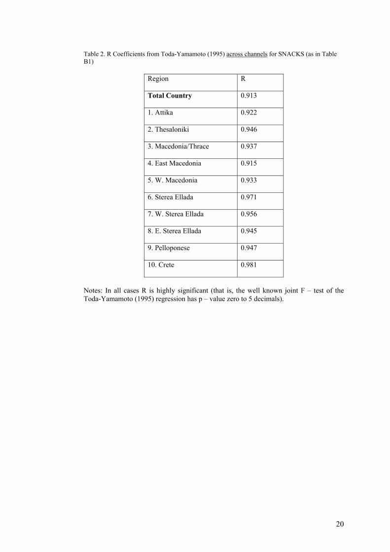
As we have explained this is wrong when, in fact, prices are I(1) and co-integrated, that is precisely when the products are indeed in the same market. Now the critical question is the following: Suppose we have two series X and Y and we want to compute their correlation. Recognizing the possible presence of integration and / or cointegration, without taking explicit position and doing tests, is it possible to compute the correct correlation coefficient? The answer (as shown by Toda and Yamamoto, 1995) is positive. What we have to do is compute the regression Y = α + βX augmenting by leads and lags of Χ and Y. In technical terms we have to compute this regression32:
1 1
L L
t t l t l l t l tl l
Y X Y X eα β γ δ− −= =
= + + + +∑ ∑ (3)
where L should be greater than or equal to the maximum order of integration of X and Y. This gives the results in Table 2.
Table 2. R Coefficients from Toda-Yamamoto (1995) across channels for SNACKS (as in Table B1)
Let us now do the equivalent of Table B2. Here we need the correlation of log prices between Snacks and Nuts for the whole market.
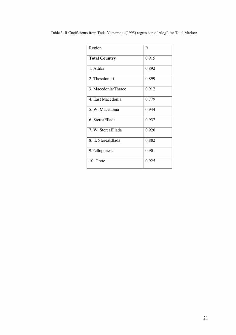
Table 3. R Coefficients from Toda-Yamamoto (1995) regression of ΔlogP for Total Market.
In Table 3 we provide the R coefficients for the regression logPSNACKS = α + βlogPNUTS no matter whether there is non-stationarity or co-integration. Apparently the correlations are quite large. Indeed the minimum R is 0.75 and the maximum R is about 0.94.
3.3.2 Granger causality results
Granger causality tests have a long history in applied econometrics. With I(1) variables the Granger test is expected to reject causality and under cointegration it will indicate the presence of causality, as it should, in the right direction (that is, from X to Y if that is indeed the direction of causation). Our results, reported in Table B.3 (in Appendix B.2) show that in most cases we do indeed have causality which accords with the claim that the products are in the same market. Of course the sample size is small but such findings are at least re-assuring in the sense that OLS-Granger estimates converge at the fast rate of T-1.
3.3.3 Unit root tests results
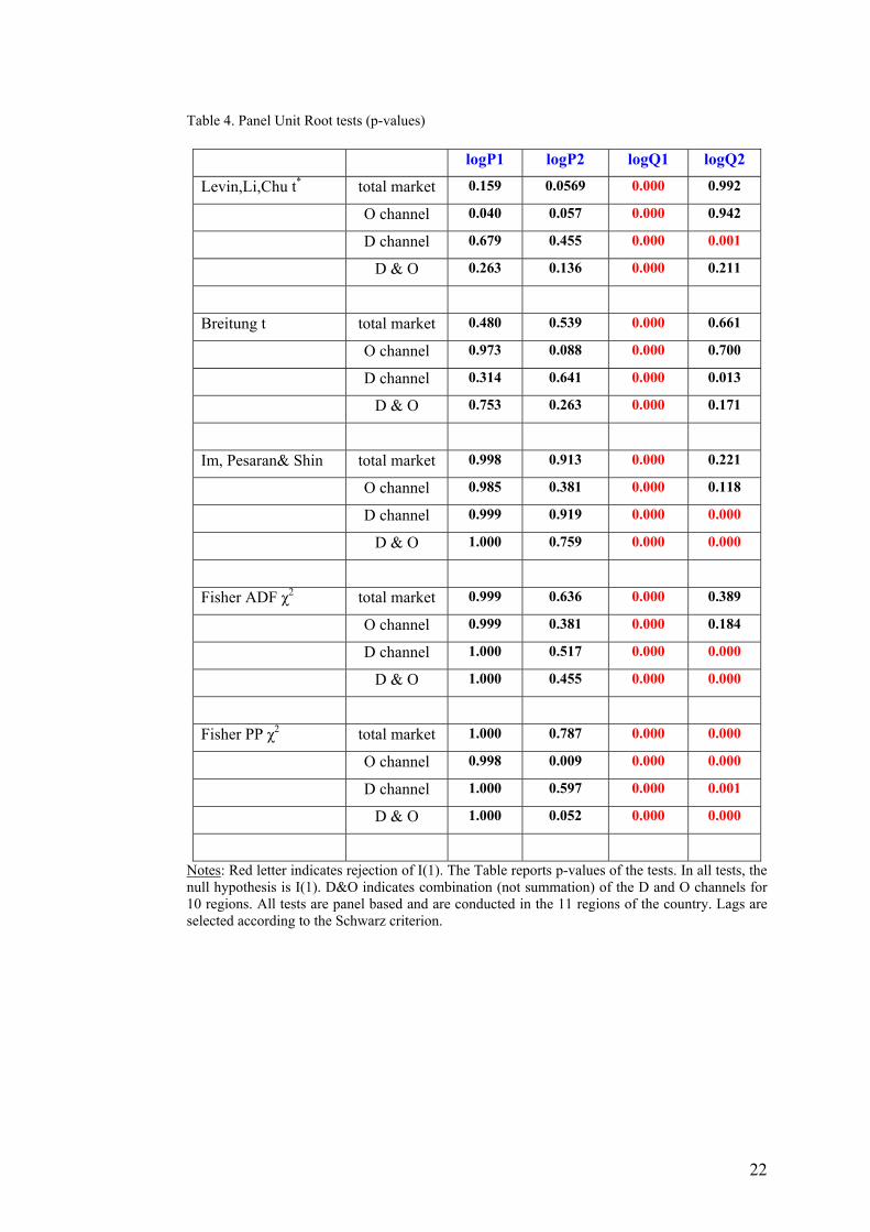
Individual—time series unit roots at the regional level indicate that log prices are indeed non—stationary of the I(1) variety. The results for the ADF and KPSS tests are reported in Appendix C (Table C1) where we also report the results of the Elliott-Rothenberg-Stock (1996) DF-GLS test (Table C2). Here we will focus on the panel unit root tests using regions as different units of the panel. The results are reported in Tables 4 and 5 below. 32 In all cases we set L=2. The results were not found to be different when L=1.
12
Table 4. Panel Unit Root tests
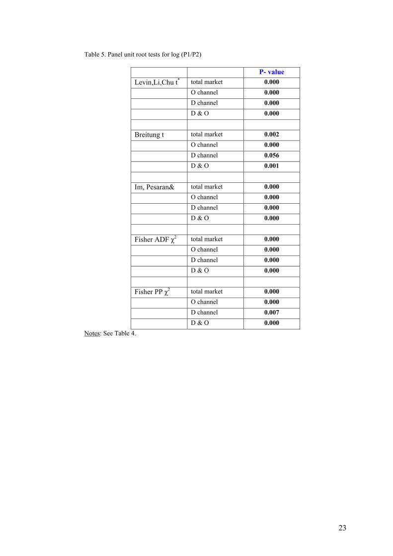
Table 5. Panel unit root tests for log (P1/P2) Graphs33 indicate that we should allow for a different regional constant but no
trend. From the panel results it is clear that the two products belong in the same market since log prices are I(1) but their difference (the log ratio of the two prices) is stationary.
Results from the more powerful Elliot-Rothenberg-Stock (1996) point-optimal tests are reported in Appendix C (Table C3). Again the message is the same as with the other unit root tests in the sense that individual price series are I(1) but their differences, more often than not, are stationary.
3.3.4 Cointegration tests results
The Johansen test
To test for cointegration between the two prices for each regions, the maximum likelihood methodology developed by Johansen (1991) is used.
The individual cointegration results are reported in Appendix D and show that in most cases prices are cointegrated. In particular, the table reports the cointegration results of Johansen’s “trace statistics” (Table D1). The tests are conducted for the totals of the three markets, Total, DTS and OT. In the first column, we write the trace statistics. The second column is the p-value associated with the null that there is at most one cointegrating relationship. Specific models and lags are selected according to the Schwarz criterion. We have “linear trend, intercept no trend model” for Total Market, and “linear trend, intercept and trend” for OT and DTS. For OT, choosing a lag which is greater by 1, the p-values become 0.0191 and 0.498 so the result that we have cointegration is strengthened. The overall result is that prices are cointegrated.
Panel cointegration tests
In this part, we conduct panel cointegration tests first to test if the two price series are cointegrated and thus, in essence, whether the two products belong to the same market, and secondly to test for the existence of long-run relations between the variables of the demand function; the latter is required before we can proceed to estimating the demand function.
The important issue of extending cointegration to allow for panels has been addressed by Pedroni (2000, 2001). We use panel cointegration tests because they offer beneficial results in terms of power. Pedroni (1999) proposed seven tests following asymptotically a standard normal distribution. First of all he constructs three non-parametric tests that correct for serial correlation, a) a non-parametric variance ratio statistic, b) a test analogous to the Phillips and Perron (PP) rho-statistic and c) a test analogous to the PP t-statistic. These panel statistics are based on pooling the data along the within dimension of the panel. He also constructs a fourth parametric test similar to the ADF-type test. The other three statistics are referred to as group-mean panel cointegration statistics.The first two of the group-mean panel cointegration statistics are panel versions of the Phillips
33 Not reported here, available on editor’s request.
13
and Perron ρ- and t-statistics, respectively. The third is a group-mean ADF test analogous to the Im et al. (2003) panel unit root test.
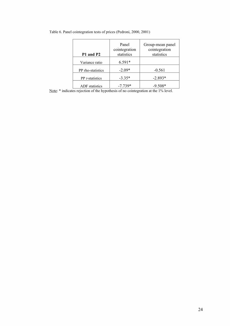
The results in Tables (6 and 7) show first that panel cointegration statistics provide evidence to support the existence of a structural relationship between the two prices (table 6) and of long run relations between the variables of the demand function (Table 7). Table 6. Panel cointegration tests of prices (Pedroni, 2000, 2001)
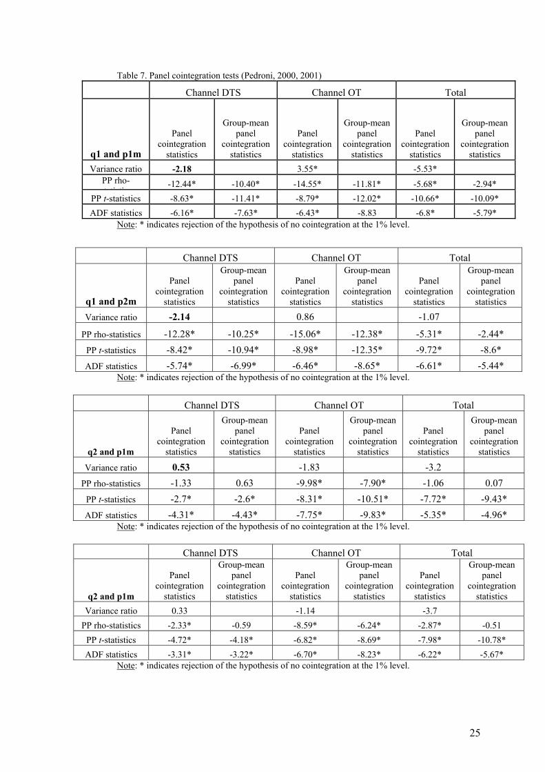
Table 7. Panel cointegration tests (Pedroni, 2000, 2001)
4. Concluding remarks Market share is the most important indicator of market power used by
Competition Authorities. To measure it correctly it is absolutely essential to define accurately relevant products and geographical markets. To do so, it is standard to use the SSNIP test, but as explained in the introduction this has serious drawbacks in cases of dominant firms. While in this paper we have undertaken the SSNIP test we also have proposed and then applied a large number of other quantitative tests at the disposal of economists in an effort to delineate the relevant antitrust market of Savory Snacks - one of the most investigated markets worldwide. Our analysis provides for the first time a detailed application and comparison of the complete set of all the quantitative tests that have been proposed at various times by economists for defining antitrust markets. In particular, we undertook apart from the SSNIP, price correlation and Granger causality tests a large number of price co-movement tests, in the light of developments in econometric techniques, using Greek bimonthly data from this market for the period 2005 – 2010. During this period, PepsiCo has been the largest player in Greece with market shares of over 70% in narrowly defined markets but less than 50% in widely defined markets. The results of our extensive tests indicate that a wide market definition is more appropriate in the Savory Snacks market.

14
References Baker JB, Bresnahan TF (1988) Estimating the residual demand curve facing a single firm. International Journal of Industrial Organization 6:283-300. doi: 10.1016/S0167-7187(88)80012-2 Bishop S, Walker M (2002) The economics of EC competition law, concepts, application and measurement. Sweet and Maxwell, London Boshoff W (2012) Advances in price-time-series tests for market definition. Stellenbosh Economic Working Papers: 01/11 Breitung J (2000) The local power of some unit root tests for pane data. In: Baltagi B (ed) Nonstationary panels, panel cointegration, and dynamic panels, Advances in Econometrics 15. JAI Press, Amsterdam, pp 161-178 Commission Notice on the definition of relevant market for the purposes of Community Competition Law (97/C 372/03), 09.12.97 available in http://europa.eu/legislation_summaries/competition/firms/l26073_en.htm Coe P, Krause D (2008) An analysis of price-based tests of antitrust market delineation. Journal of Competition Law & Economics 4:983-1007 Dickey D A, Fuller W A (1979) Distribution of the estimators for autoregressive time series with a unit root. Journal of the American Statistical Association 74:427-431 Elliot G, Rothenberg T J, Stock J H (1996) Efficient tests for an autoregressive unit root. Econometrica 64:813-836 Engle RF, Granger C W J (1987) Co-integration and error correction: representation, estimation, and testing. Econometrica 55:251–276 Euromonitor international database (www.euromonitor.com) European Snack Association international database (www.esa.org) Forni M (2004) Using stationarity tests in antitrust market definition. American Law and Economics Review 6:441-464.doi:10.1093/aler/ahh007 Hadri K (2000) Testing for stationarity in heterogeneous panel data. Econometrics Journal 3:148-161. doi: 10.1111/1368-423X.00043 Hausman J, Leonard Gr (2005) Competitive analysis using a flexible demand specification. Journal of Competition Law and Economics 1:279–301. doi: 10.1093/joclec/nhi008 Hosken D, Taylor Chr (2004) Discussion of ‘Using stationarity tests in antitrust market definition’. American Law and Economics Review 6:465-475. doi: 10.1093/aler/ahh008 Im K S, Pesaran M H, Smith Y (2003), Testing for unit roots in heterogeneous panels. Journal of Econometrics 115:53-74 Johansen S (1991) Estimation and hypothesis testing of cointegration vectors in Gaussian vector autoregressive models. Econometrica 59:1551–1580 Johansen S (1995) Likelihood-based inference in cointegrated vector autoregressive models. Oxford University Press, Oxford. doi:10.1093/0198774508.001.0001 Kamerschen D R, Kohler J (1993) Residual demand analysis of the ready-to-eat breakfast cereal market. The Antitrust Bulletin 38: 903-42 Kantar World Panel (2009) Research: Core salty & nuts Interaction

15
Kendall M, Stuart A (1977) The advanced theory of statistics, volume 1, fourth edition. Griffin: London Kwiatkowski D, Phillips P C B, Schmidt P, Shin Y (1992) Testing the null hypothesis of stationarity against the alternative of a unit root: How sure are we that economic time series have a unit root? Journal of Econometrics 54:159-178 Levin A, Lin C F, Chu C (2002) Unit root tests in panel data: asymptotic and finite sample properties. Journal of Econometrics 108:1-24 MacKinnon J (1996) Numerical distribution functions for unit root and cointegration tests. Journal of Applied Econometrics 11:601-618. doi: 10.1002/(SICI)1099-1255(199611)11:6<601::AID-JAE417>3.0.CO;2-T Maddala G S, Wu S (1999) A comparative study of unit root tests with panel data and a new simple test. Oxford Bulletin of Economics and Statistics 61:631-652. doi: 10.1111/1468-0084.0610s1631 Motta M, (2004), Competition policy. Theory and practice. Cambridge University Press, Cambridge Muris T, Scheffman D, Spiller P (1993) Strategy, structure, and antitrust in the carbonated soft-drink industry. Quorum Books, Westport CT Newey W, West K (1994) Automatic lag selection in covariance matrix estimation. Review of Economic Studies 61:631–653 O’Donoghue R, Padilla J (2007) The law and economics of Article 82 EC. Hart Publishing, Oxford Pedroni P (2000) Fully modified OLS for heterogeneous cointegrated panels. In: Baltagi B H, Fomby T B and Hill R C (eds) Nonstationary panels, panel cointegration and dynamic panels. Advances in Econometrics. Vol. 15, pp 93-130. Elsevier Science, Amsterdam. doi: 10.1016/S0731-9053(00)15004-2 Phillips P C B and Hansen B E (1990) Statistical inference in instrumental variable regression with I(1) processes. Review of Economic Studies 57: 99-125 Pedroni P (2001) Purchasing power parity tests in cointegrated panels. Review of Economics and Statistics 83:727-731 Pesaran M H, Shin Y (1999) An autoregressive distributed lag modelling approach to cointegration analysis. In: Strom S (ed) Econometrics and Economic Theory in the 20th Century: The Ragnar Frisch Centennial Symposium. Cambridge University Press, Cambridge, pp 371-413 Pesaran M H, Shin Y, Smith R (2001) Bounds testing approaches to the analysis of level relationships. Journal of Applied Econometrics 16:289-326. doi: 10.1002/jae.616 Phillips P C B (1998) New tools for understanding spurious regressions. Econometrica 66:1299-1326 Phillips PCB, Perron P (1988)Testing for a unit root in a time series regression. Biometrika 75:335-346. doi: 10.1093/biomet/75.2.335 Salvetti & Llombart research (December 2004) on the delineation of the Savory Snacks market, Greece Sims C A (1980) Macroeconomics and reality. Econometrica 48:1-48 Stigler G J, Sherwin R A (1985) The extent of the market. The Journal of Law and Economics 28:555-585

16
Stock JH, Watson M (1993) A simple estimator of cointegrating vectors in higher order integrated systems. Econometrica 61:783-820 Toda HY, Phillips P C B (1993) Vector autoregressions and causality. Econometrica 61:1367-1393. Toda, H.Y. and Yamamoto (1995) Statistical inference in vector autoregressions with possibly integrated processes. Journal of Econometrics 66:225-250 Werden G J and Froeb L M (1993) Correlation, causality and All that jazz: The inherent shortcomings of price tests for antitrust market delineation. Review of Industrial Organization 8:329-353
17
Diagram 1: Core Salty Market – TASTY Market Share in Total MarketVolume (%)
18
Diagram 2: Core Salty and Nuts Market – TASTY Market Share in Total MarketVolume (%)
19
Table 1: FMOLS Results
Table 1: FMOLS Results Fully modified OLS estimates p1m p2m
q1 -1.70 [-4.55] 0.57 [3.67] Channel DTS q2 0.61 [4.11] -1.82 [-7.32]
q1 -1.73 [-9.10] 0.67 [2.12] Channel OTS q2 0.34 [4.33] -1.81 [-3.44]
q1 -1.73 [-5.17] 0.60 [3.30] Total q2 0.52 [4.10] -1.79 [-4.55]
Notes: The table provides estimates for channels DTS and OTS and for the total market by treating separate regions of the country as different units of the panel.
20
Table 2. R Coefficients from Toda-Yamamoto (1995) across channels for SNACKS (as in Table B1)
Region R
Total Country 0.913
1. Attika 0.922
2. Thesaloniki 0.946
3. Macedonia/Thrace 0.937
4. East Macedonia 0.915
5. W. Macedonia 0.933
6. Sterea Ellada 0.971
7. W. Sterea Ellada 0.956
8. E. Sterea Ellada 0.945
9. Pelloponese 0.947
10. Crete 0.981
Notes: In all cases R is highly significant (that is, the well known joint F – test of the Toda-Yamamoto (1995) regression has p – value zero to 5 decimals).
21
Table 3. R Coefficients from Toda-Yamamoto (1995) regression of ΔlogP for Total Market:
Region R
Total Country 0.915
1. Attika 0.892
2. Thesaloniki 0.899
3. Macedonia/Thrace 0.912
4. East Macedonia 0.779
5. W. Macedonia 0.944
6. StereaEllada 0.932
7. W. StereaEllada 0.920
8. E. StereaEllada 0.882
9.Pelloponese 0.901
10. Crete 0.925
22
Table 4. Panel Unit Root tests (p-values)
logP1 logP2 logQ1 logQ2
Levin,Li,Chu t* total market 0.159 0.0569 0.000 0.992
O channel 0.040 0.057 0.000 0.942
D channel 0.679 0.455 0.000 0.001
D & O 0.263 0.136 0.000 0.211
Breitung t total market 0.480 0.539 0.000 0.661
O channel 0.973 0.088 0.000 0.700
D channel 0.314 0.641 0.000 0.013
D & O 0.753 0.263 0.000 0.171
Im, Pesaran& Shin total market 0.998 0.913 0.000 0.221
O channel 0.985 0.381 0.000 0.118
D channel 0.999 0.919 0.000 0.000
D & O 1.000 0.759 0.000 0.000
Fisher ADF χ2 total market 0.999 0.636 0.000 0.389
O channel 0.999 0.381 0.000 0.184
D channel 1.000 0.517 0.000 0.000
D & O 1.000 0.455 0.000 0.000
Fisher PP χ2 total market 1.000 0.787 0.000 0.000
O channel 0.998 0.009 0.000 0.000
D channel 1.000 0.597 0.000 0.001
D & O 1.000 0.052 0.000 0.000
Notes: Red letter indicates rejection of I(1). The Table reports p-values of the tests. In all tests, the null hypothesis is I(1). D&O indicates combination (not summation) of the D and O channels for 10 regions. All tests are panel based and are conducted in the 11 regions of the country. Lags are selected according to the Schwarz criterion.
23
Table 5. Panel unit root tests for log (P1/P2)
P- value Levin,Li,Chu t* total market 0.000
Ο channel 0.000
D channel 0.000
D & O 0.000
Breitung t total market 0.002
O channel 0.000
D channel 0.056
D & O 0.001
Im, Pesaran& total market 0.000
O channel 0.000
D channel 0.000
D & O 0.000
Fisher ADF χ2 total market 0.000
O channel 0.000
D channel 0.000
D & O 0.000
Fisher PP χ2 total market 0.000
O channel 0.000
D channel 0.007
D & O 0.000 Notes: See Table 4.
24
Table 6. Panel cointegration tests of prices (Pedroni, 2000, 2001)
P1 and P2
Panel cointegration
statistics
Group-mean panel cointegration
statistics
Variance ratio 6.591*
PP rho-statistics -2.09* -0.561
PP t-statistics -3.35* -2.893*
ADF statistics -7.739* -9.508* Note: * indicates rejection of the hypothesis of no cointegration at the 1% level.
25
Table 7. Panel cointegration tests (Pedroni, 2000, 2001)
Channel DTS Channel OT Total
q1 and p1m
Panel cointegration
statistics
Group-mean panel
cointegration statistics
Panel cointegration
statistics
Group-mean panel
cointegration statistics
Panel cointegration
statistics
Group-mean panel
cointegration statistics
Variance ratio -2.18 3.55* -5.53* PP rho-t ti ti
-12.44* -10.40* -14.55* -11.81* -5.68* -2.94* PP t-statistics -8.63* -11.41* -8.79* -12.02* -10.66* -10.09* ADF statistics -6.16* -7.63* -6.43* -8.83 -6.8* -5.79*
Note: * indicates rejection of the hypothesis of no cointegration at the 1% level.
Note: * indicates rejection of the hypothesis of no cointegration at the 1% level.
Channel DTS Channel OT Total
q2 and p1m
Panel cointegration
statistics
Group-mean panel
cointegration statistics
Panel cointegration
statistics
Group-mean panel
cointegration statistics
Panel cointegration
statistics
Group-mean panel
cointegration statistics
Variance ratio 0.53 -1.83 -3.2 PP rho-statistics -1.33 0.63 -9.98* -7.90* -1.06 0.07
PP t-statistics -2.7* -2.6* -8.31* -10.51* -7.72* -9.43* ADF statistics -4.31* -4.43* -7.75* -9.83* -5.35* -4.96*
Note: * indicates rejection of the hypothesis of no cointegration at the 1% level.
Channel DTS Channel OT Total
q2 and p1m
Panel cointegration
statistics
Group-mean panel
cointegration statistics
Panel cointegration
statistics
Group-mean panel
cointegration statistics
Panel cointegration
statistics
Group-mean panel
cointegration statistics
Variance ratio 0.33 -1.14 -3.7 PP rho-statistics -2.33* -0.59 -8.59* -6.24* -2.87* -0.51
PP t-statistics -4.72* -4.18* -6.82* -8.69* -7.98* -10.78* ADF statistics -3.31* -3.22* -6.70* -8.23* -6.22* -5.67*
Note: * indicates rejection of the hypothesis of no cointegration at the 1% level.
Channel DTS Channel OT Total
q1 and p2m
Panel cointegration
statistics
Group-mean panel
cointegration statistics
Panel cointegration
statistics
Group-mean panel
cointegration statistics
Panel cointegration
statistics
Group-mean panel
cointegration statistics
Variance ratio -2.14 0.86 -1.07
PP rho-statistics -12.28* -10.25* -15.06* -12.38* -5.31* -2.44* PP t-statistics -8.42* -10.94* -8.98* -12.35* -9.72* -8.6* ADF statistics -5.74* -6.99* -6.46* -8.65* -6.61* -5.44*
26
APPENDIX A. Competition Cases Concerning the Savory Snacks market
We examined 18 different antitrust investigations of the savory snacks market that
were undertaken from national Antitrust Authorities and the European Commission. Interestingly in half of these cases the Competition Authorities go for a wide definition of the market, while on the other half they go for a narrow definition.
A wide definition of the savory snacks market was adopted by the Competition Authorities in UK (3 cases), Belgium (2 cases), Poland and Netherlands as well as in two cases investigated by the European Commission. Despite the differences in national consumption habits, in all these cases a high demand side substitutability was presumed. According to the opinion of these Authorities ALL Savory snacks cover a common need, consist of an impulse purchase, are consumed usually between meals under the same eating occasions and are sold in the same placement on the shelves, all factors that indicate that they constitute a single market.
The savory snacks market, as defined in cases where the market is defined broadly usually includes chips, extruded snacks and nuts. A brief description of the cases follows:
Nabisco Brands / Huntley & Palmer (UK, 1982) is the oldest antitrust case regarding the savory snacks market. In 1982 the UK Monopolies and Mergers Commission (MMC) examined the takeover bid of Nabisco Brands for Huntley and Palmer Foods34. The MMC defined the market of savory snacks to include crisps, snacks (cereal or potato based) and nuts with the exception of nuts sold as cooking ingredients.35
Frito Lay Trading Co GmbH / Golden Wonder Group Ltd (UK, 2002)36is another merger case in UK in 2002. The parties overlapped in the manufacture and supply of savory snacks in UK37. The General Director of Fair Trading in his report to the Secretary of State for Trade and Industry in July 2002 stated that the savory snacks market at its widest consists of nuts, crisps, extracted, corn and baked snacks38 (as the MMC has defined in Nabisco and H&P case).
In 1992 and 1999 the European Commission faced two cases where the companies were active in the snack foods sector and adopted a wide definition of the relevant market including all savory snacks.
PepsiCo / General Mills39 (EC, 1992). In 1992 the Commission examined the notification of a proposed concentration where General Mills Inc. and PepsiCo Inc – two US based companies - would transfer all and parts, respectively, of their European snack 34Nabisco is a US company with a strong presence in biscuit, cereal based and peanut based products, confectionary, snacks and alcoholic beverages market while Huntley and Palmer was the second largest UK biscuits and snack manufacturer. 35The MMC also noted the inter-relation between biscuits, snacks and confectionary markets since these are impulse purchases and are usually eaten between meals but significant differences like prices, place of sale, taste, consumer age (adults and children) nature of wrapping and need of preparation before eating, were also found. 36Proposed acquisition by Frito Lay Trading Co GmbH, a subsidiary of PepsicoInc, of certain assets of the Golden Wonder Group Ltd, namely the Wotsits brand and associated production and distribution facilities, No. ME/1302/02. 37Frito Lay Trading Co GmbH is a subsidiary of PepsiCo Inc, a major food and drink supplier, with a substantial presence in salty snacks, refreshment beverages and branded juices. Golden Wonder Group Ltd is a manufacturer and distributor of bagged snacks. 38Third parties have also suggested that there may be a distinction between sales in savory snack multipacks (weekly shop) and sales of single packs (impulsive purchase). However, the MMC found that either sector will be immune from competition from the other since suppliers sell in both sectors. 39Case No IV / M.232 – PEPSICO / GENERAL MILLS, Date: 05.08.1992, Document No. 392M0232.
27
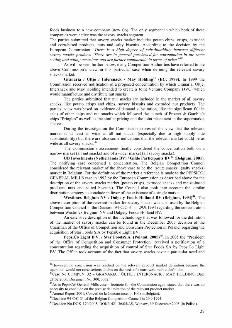
foods business to a new company (new Co). The only segment in which both of these companies were active was the savory snacks segment. The parties submitted that savory snacks market includes potato chips, crisps, extruded and corn-based products, nuts and salty biscuits. According to the decision by the European Commission “There is a high degree of substitutability between different savory snacks products. There are in general purchased for consumption in the same setting and eating occasions and are further comparable in terms of price.”40
As will be seen further below, many Competition Authorities have referred to the above Commission’s view in this particular case when defining the relevant savory snacks market.
Granaria / Ültje / Intersnack / May Holding41 (EC, 1999). In 1999 the Commission received notification of a proposed concentration by which Granaria, Ültje, Intersnack and May Holding intended to create a Joint Venture Company (JVC) which would manufacture and distribute nut snacks.
The parties submitted that nut snacks are included in the market of all savory snacks, like potato crisps and chips, savory biscuits and extruded nut products. The parties’ view was based on evidence of demand substitution, like the significant fall in sales of other chips and nut snacks which followed the launch of Procter & Gamble’s chips “Pringles” as well as the similar pricing and the joint placement in the supermarket shelves.
During the investigation the Commission expressed the view that the relevant market is at least as wide as all nut snacks (especially due to high supply side substitutability) but there are also some indications that the relevant market could be as wide as all savory snacks.42
The Commission’s assessment finally considered the concentration both on a narrow market (all nut snacks) and of a wider market (all savory snacks).
UB Investments (Netherlands BV) / Gilde Participants BV43 (Belgium, 2001). The notifying case concerned a concentration. The Belgian Competition Council considered the relevant market of the above case to be the “zoute snacks” (salty snacks) market in Belgium. For the definition of the market a reference is made to the PEPSICO/ GENERAL MILLS case in 1992 by the European Commission as described above for the description of the savory snacks market (potato crisps, extruded snacks and maize-based products, nuts and salted biscuits). The Council also took into account the similar distribution strategy to conclude in favor of the existence of a single market.
Westimex Belgium NV / Dalgety Foods Holland BV (Belgium, 1994)44. The above description of the relevant market for savory snacks was also used by the Belgian Competition Council in the Decision 94-C/C-31 in 29.9.1994 regarding the concentration between Westimex Belgium NV and Dalgety Foods Holland BV.
An extensive description of the methodology that was followed for the definition of the market of savory snacks can be found in the December 2005 decision of the Chairman of the Office of Competition and Consumer Protection in Poland, regarding the acquisition of Star Foods S.A by PepsiCo Light BV.
PepsiCo Light B.V. / Star FoodsS.A. (Poland, 2005)45. In 2005 the “President of the Office of Competition and Consumer Protection” received a notification of a concentration regarding the acquisition of control of Star Foods SA by PepsiCo Light BV. The Office took account of the fact that savory snacks cover a particular need and
40However, no conclusion was reached on the relevant product market definition because the operation would not raise serious doubts on the basis of a narrowest market definition. 41Case No COMP/JV. 32 – GRANARIA / ÜLTJE / INTERSNACK / MAY HOLDING, Date 28.02.2000, Document No. 300J0032. 42As in PepsiCo/ General Mills case – footnote 8. - the Commission again stated that there was no necessity to conclude on the precise delimitation of the relevant product market. 43Annual Report 2001, Conceil de la Concurrance, p. 106 (in Belgian). 44Decision 94-C/C-31 of the Belgian Competition Council in 29.9.1994. 45Decision No.DOK-170/2005, DOK3-421-36/05/AS, Warsaw, 19 December 2005 (in Polish).
28
consumers can meet this need by using any of the salty snacks (i.e. chips, crisps, bread sticks, pretzels, salty biscuits/crackers, peanuts and pop corn) and not a particular one. Consumer surveys conducted at the request of the applicants showed that most respondents consume salty snacks while watching TV (60%), serve refreshments (39%), to satisfy their appetite (36%), consume with friends (31%). Also different types of salty snacks are regarded by the consumers as substitutes46.
There is also a note on similar packaging methods and consumption possibilities. All kinds of salty snacks feature the possibility of direct consumption as they are unpacked even though there is a wide range of pack sizes.
Surveys conducted by the Office had shown that according to sellers (retailers) salty snacks market should be regarded as a single market since all snacks have common features (reasons for consumption, place to purchase, buying impulsiveness, placement on selves). But the manufacturers – apart from the merging parties – stated that each of the segments should be treated as a separate market due to the nature and cost of production. However, this claim was not justified in the context of the whole analysis and all kinds of salty snacks counted in a single market.
PepsiCo / Duyvis (Netherlands Competition Authority, 2006)47. In 2006, the Board of Directors of the Dutch Competition Authority received a notification of a this proposed concentration. In this case the parties have indicated that “in the eyes of consumers the various products on the market for savory snacks is highly interchangeable since the moments of use, the consumer behavior and consumption locations are almost identical for the products of the different segments”. This view was confirmed by researches among customers.48
In this decision the market of chips, salty snacks, savory biscuits and other savory snacks, both branded and private labeled, “was taken as a starting point” by the Competition Authority.
Walkers Snacks Limited (UK, 2007)49. The latest antitrust case for the savory snacks market where a wide definition of the market is used took place again in UK in 2007. In the above mentioned case of Frito LayTrading Co GmbH / Golden Wonder Group Ltd merger, the report the Director General of Fair Trading noted that significant concerns had been expressed in relation to WSL's trading practices and OFT opened a case file to investigate the abuse of dominance by Walkers.
OFT considered key product characteristics, demand conditions, evidence of substitution and previous UK competition analyses in order to define the relevant market which was finally characterized as “all savory snacks”. These include potato crisps, extruded and pellet – fried snacks, corn snacks, snack nuts and certain baked products.
Contrary to the above definition of the relevant market the Competition Authorities in Italy, New Zealand, Spain, Austria and France as well as the European Commission in three cases adopted a narrow definition of the relevant market. It should be noted that in some of these cases evidence of a wider definition of the market was found but since no competition concerns could arise under a narrow definition, a wider definition would not change the outcome50. It should also be noted that in many of these cases the Authorities took into account different commodity characteristics of the products in question (eg. The Italian Competition Authority considers different nutritional capacity) as an important factor that delimits the relevant market.
4666% of the respondents regarded potato chips and other salty snacks good substitutes. The percentage was 79% for crisps and other salty snacks, 77% for salty biscuits and crackers and other salty snacks, 63% for salty sticks and other salty snacks and 72% for salty peanuts and other salty snacks. 47Case PepsiCo / Duyvis, No 5476, 24th April 2006 (in Dutch). 48In this case again, as in GRANARIA/ÜLTJE/INTERSNACK/MAY HOLDING (EC, 1999), the decline in the sales of all different segments of the savory snacks due to the introduction of Pringle by Procter & Gamble has been noted. 49 Walkers Snacks Limited, Office of Fair Trading, Decision on 3.5.2007. 50 See below case Bluebird Foods Limited / Hansells (New Zealand, 2005).
29
From 2000 to 2007 the European Commission faced three different cases regarding the manufacturing and supply of biscuits. In these cases, contrary to the above decisions, the EC regarded biscuits as a separate relevant market. In the 2007 decision EC divided this market in even more sub-segments (sweet and savory biscuits).
Nabisco / United Biscuits (EC, 2000)51. In 2000 the Commission received a notification of a proposed concentration by which the US Company Nabisco acquired control of the UK companies United Brands and Horizon52. The parties were overlapping in the production of (sweet) biscuits. According to the market investigation biscuits constitute a separate relevant market while the question of even narrower boundaries (sub-segments like sweet, chocolate-coated, other than chocolate-coated, savory biscuits) was left opened.
Orkla / Chips (EC, 2005)53. In 2005 the European Commission received a notification for the merger of Orkla and Chips54 and found that there is no overlapping between parties’ activities in snacks and salted biscuits. The market investigation confirmed the parties’ view that snacks and salted biscuits are two different markets in the Nordic countries55 since these are not consumed in the same way and under the same occasions neither are they sold in the same shelves.56
Kraft / Danone Biscuits (EC, 2007)57. The parties’ activities in this 2007 merger case were overlapping in the biscuits58 and chocolate confectionary sectors specially countlines59.
Regarding the biscuits market the notifying parties view was that biscuits are part of the overall market for snacking products. However, since in both of the previous merger cases regarding biscuits mentioned above the Commission used a narrower definition of the market, the parties assumed that that was the relevant market for biscuits.
Market investigations in Spain and Portugal have also concluded that there are different relevant markets for sweet and savory biscuits since these are generally consumed in different ways and occasions. Even if the supply side substitutability is high the producers are substantially stronger in one of these markets.
One of the European countries that have adopted a narrow definition of the savory snacks market is Italy, for the Unichips / Finanziaria / Alidolcecase, in 1993, and the Grani& Partners / Mitica Food cases ten years later, in 2003.
UnichipsFinanziaria / Alidolce60 (Italy, 1993). In 1992 UnichipsFinanziaria communicated to the Authority its intention to acquire the entire share capital of
51Case No COMP/M.1920 – NABISCO / UNITED BISCUITS, Document No. 300M1920, 5/5/2000. 52 The geographic market for biscuits affected by the concentration was regarded as national. 53Case No. COMP/M.3658 – ORKLA / CHIPS, Document No. 32005M3658, 3/3/2005. 54The Commission distinguished the production of food dedicated to retailers and food dedicated to food service sector (hotels, restaurants etc). 55 The Commission found that the relevant geographic markets for the food products under investigation were probably national (Nordic countries) in scope. 56The Decision also describes the market investigation for the three product categories concerned by the transaction: frozen ready meals, frozen potato products and herrings, Baltic herrings and anchovies. 57Case No. COMP/M.4824 –KRAFT / DANONE BISCUITS, Document No. 32007M4824, 9.11.2007. 58In particular the parties were overlapping in the biscuit market in Spain and Portugal. 59The parties were overlapping in the countlines market in Belgium, Czech Republic, Slovakia and Hungary. The Commission defined product markets with regard to each of the four countries. In Belgium, Czech Republic and Slovakia the precise market definition was left open while in Hungary the Commission defined separate markets for countlines and other chocolate confectionaries. 60 Case No. C714, UNICHIPS FINANZIARIA/ALIDOLCE, L'AutoritádellaConcorrenza e del Mercato, Italy, 23.02.1993 (in Italian).
30
ALIDOLCE. The Italian Competition Authority has defined separate markets for chips, extruded snacks, salty biscuits and shelled snacks, although some degree of substitutability was not excluded.
According to the investigation by the Authority the commodity profile of the products is different defining different taste and perceptions of the consumers regarding naturalness, digestibility and nutritional capacity. Also, different products remained different time on the shelves of the stores61 something that was considered as evidence of different consumption habits and duration at stock for each of these products.
With regard to production technology, the analysis of specific methods of production used in savory snacks highlighted the existence of partial differentiation and with regard to the price the savory snacks industry analysis showed substantial independence between different products.
Finally, in relation to product placement in retail outlets it was found that potato chips and extruded products are marketed in the same space, while the other snacks, “mainly intended to complement the cocktail function”, are displayed in different areas of the store.
Grani&Partners / MiticaFood62 (Italy, 2003). The transaction notified consisted of the acquisition of the 60% of the share capital of Mitica. In this case again the differences in the components of production the different placement on shelves etc led to the conclusion that the relevant markets for French fries, salted snacks, extruded snacks and the pretzels are distinct although they have some degree of substitutability.
Bluebird Foods Limited / Hansells (New Zealand, 2005)63. The case regarded the acquisition by Bluebird Foods Limited of certain businesses and assets of Hansells (NZ) Limited and PLC (NZ) Limited. The Commerce Commission of New Zealand defined the relative market of savory snacks to include potato chips, corn chips and extrusions due to the high degree of the demand side substitutability64 since these products cover the same need and have similar price.
However, the Commission did not consider it appropriate to include nuts in the relative market, as has been claimed by the Applicant, and considered that if “there are no competition concerns in the narrowly defined market, there are unlikely to be any in a more broadly defined market that included nuts”.
Panrico / Kraft (Spain, 2008)65. Based on the above mentioned decision of the European Commission for Kraft –Danone, the Directorate of Research in Spain decided to analyse the effects of this merger on the markets of cookies and crackers leaving open the possibility of segmenting these markets additionally due to the absence of competition problems irrespective of the definition adopted.
Kelly GmbH / IntersnackKnabbergebäck GmbH &Co KG (Austria, 2008)66. The Cartel Court of Austria released its decision of 03.03.2008 regarding the above merger. The Cartel Court has considered in its decision the salty snacks "except of nuts" as a relevant product market. The issue of whether manufacturers and private label brands are attributable to the same market was left open.
IK Invest BV / Snack International Développement II / L FinancièreAuroise (France, 2010)67. This is one of the most recent decisions where a narrow definition of
61For example chips remain for 6 months duration while other products for 12 months. 62Case No. C5946 - GRANI & PARTNERS/MITICA FOOD, L'AutoritádellaConcorrenza e del Mercato, Italy, 17/07/2003 (in Italian). 63 Decision No. 560, Bluebird Foods Limited / Hansells, Commerce Commission, New Zealand, 5.10.2005. 64The Commission found that there is only a limited degree of supply side substitutability, since the production process between potato chips and corn chips is similar only at the final stages. 65Case No. C-0069/08, PANRICO/KRAFT, Comisíon De La CompetenciaResolución, Spain, 05.06.2008 (in Spanish). 66Austrian Competition Authority, 3.3.2008. 67Decision No 10-DCC-170, IK Invest BV/Snack International Développement II/L FinancièreAuroise, 24.11.2010, Authorité de la Concurrence (in French).
31
the relevant market of crackers (“biscuitsaperitifs”) was used. The Authority, while leaving the question open, did not consider it appropriate to distinguish between different types of crackers (seeds, tiles, crackers ...) or between private label and manufacturer brands.
APPENDIX B1. Values of correlation coefficients
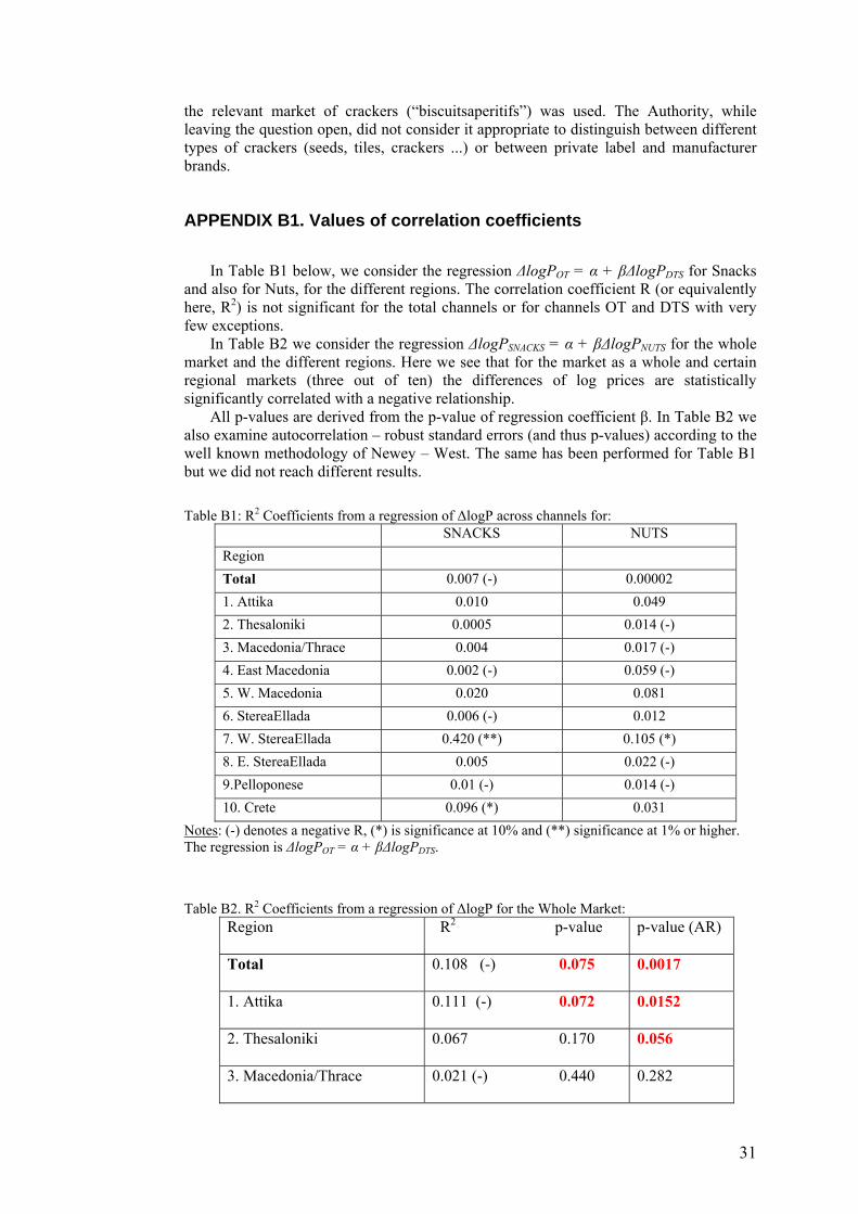
In Table B1 below, we consider the regression ΔlogPΟΤ = α + βΔlogPDTS for Snacks
and also for Nuts, for the different regions. The correlation coefficient R (or equivalently here, R2) is not significant for the total channels or for channels OT and DTS with very few exceptions.
In Table B2 we consider the regression ΔlogPSNACKS = α + βΔlogPNUTS for the whole market and the different regions. Here we see that for the market as a whole and certain regional markets (three out of ten) the differences of log prices are statistically significantly correlated with a negative relationship.
All p-values are derived from the p-value of regression coefficient β. In Table B2 we also examine autocorrelation – robust standard errors (and thus p-values) according to the well known methodology of Newey – West. The same has been performed for Table B1 but we did not reach different results.
Table B1: R2 Coefficients from a regression of ΔlogP across channels for:
SNACKS NUTS Region Total 0.007 (-) 0.00002 1. Attika 0.010 0.049 2. Thesaloniki 0.0005 0.014 (-) 3. Macedonia/Thrace 0.004 0.017 (-) 4. East Macedonia 0.002 (-) 0.059 (-) 5. W. Macedonia 0.020 0.081 6. StereaEllada 0.006 (-) 0.012 7. W. StereaEllada 0.420 (**) 0.105 (*) 8. E. StereaEllada 0.005 0.022 (-) 9.Pelloponese 0.01 (-) 0.014 (-) 10. Crete 0.096 (*) 0.031
Notes: (-) denotes a negative R, (*) is significance at 10% and (**) significance at 1% or higher. The regression is ΔlogPΟΤ = α + βΔlogPDTS.
Table B2. R2 Coefficients from a regression of ΔlogP for the Whole Market: Region R2 p-value p-value (AR)
Total 0.108 (-) 0.075 0.0017
1. Attika 0.111 (-) 0.072 0.0152
2. Thesaloniki 0.067 0.170 0.056
3. Macedonia/Thrace 0.021 (-) 0.440 0.282

32
4. East Macedonia 0.102 (-) 0.085 0.001
5. W. Macedonia 0.00 (-) 0.96 0.95
6. StereaEllada 0.004 (-) 0.73 0.60
7. W. StereaEllada 0.01 (-) 0.60 0.302
8. E. StereaEllada 0.00 0.97 0.98
9.Pelloponese 0.00 (-) 0.85 0.783
10. Crete 0.036 0.31 0.129
Notes: (-) denotes a negative R The regression is ΔlogPSNACKS = α + βΔlogPNUTS. Red color indicates significance at the level indicated or higher (e.g. 0.075 denotes significance at level 7,5%, 10% etc). AR means autocorrelation – robust. Red color indicates significance.
One important question in empirical Industrial Organisation is what values of correlation coefficients are “small”. From the data on total market we get the following results.
DependentVariable: LD1P1 Method: LeastSquares Sample (adjusted): 2000Q2 2007Q3 Includedobservations: 30 afteradjustments
Variable Coefficient Std. Error t-Statistic C 0.102893 0.115276 0.892582
LD1P1(-1) 0.959204 0.048430 19.80613
R-squared 0.933378 Adjusted R-squared 0.930999 Durbin-Watsonstat 1.698816 Meandependentvar 2.385368 S.D. dependentvar 0.058937 Prob (F-statistic) 0.000000
The constant term is not statistically significant while the value of ρ is close to 1. according to the ADF test the series is I(1). Suppose we construct a series X as
1 0,015t t tX X e−= + , where ( )~ 0,1te IIDN . Let us also construct the second price
(logP2, orΥ) as 0,03t t tY X v= + , and ( )~ 0,1tv IIDN , as our estimates show. The question is then what kinds of correlation coefficients we should expect. Given our sample size, n=30, 100,000 Monte Carlo simulations provide the results shown in the figures below.
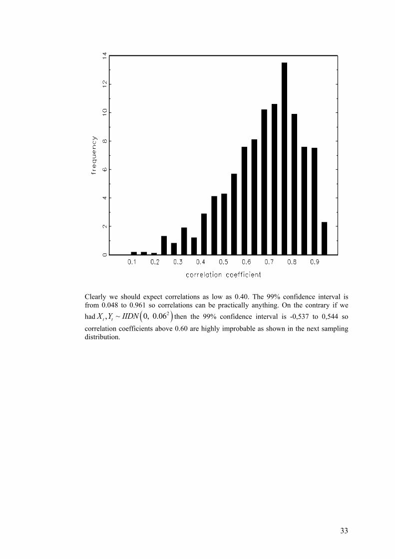
33
Clearly we should expect correlations as low as 0.40. The 99% confidence interval is from 0.048 to 0.961 so correlations can be practically anything. On the contrary if we had ( )2, ~ 0, 0.06t tX Y IIDN then the 99% confidence interval is -0,537 to 0,544 so
correlation coefficients above 0.60 are highly improbable as shown in the next sampling distribution.
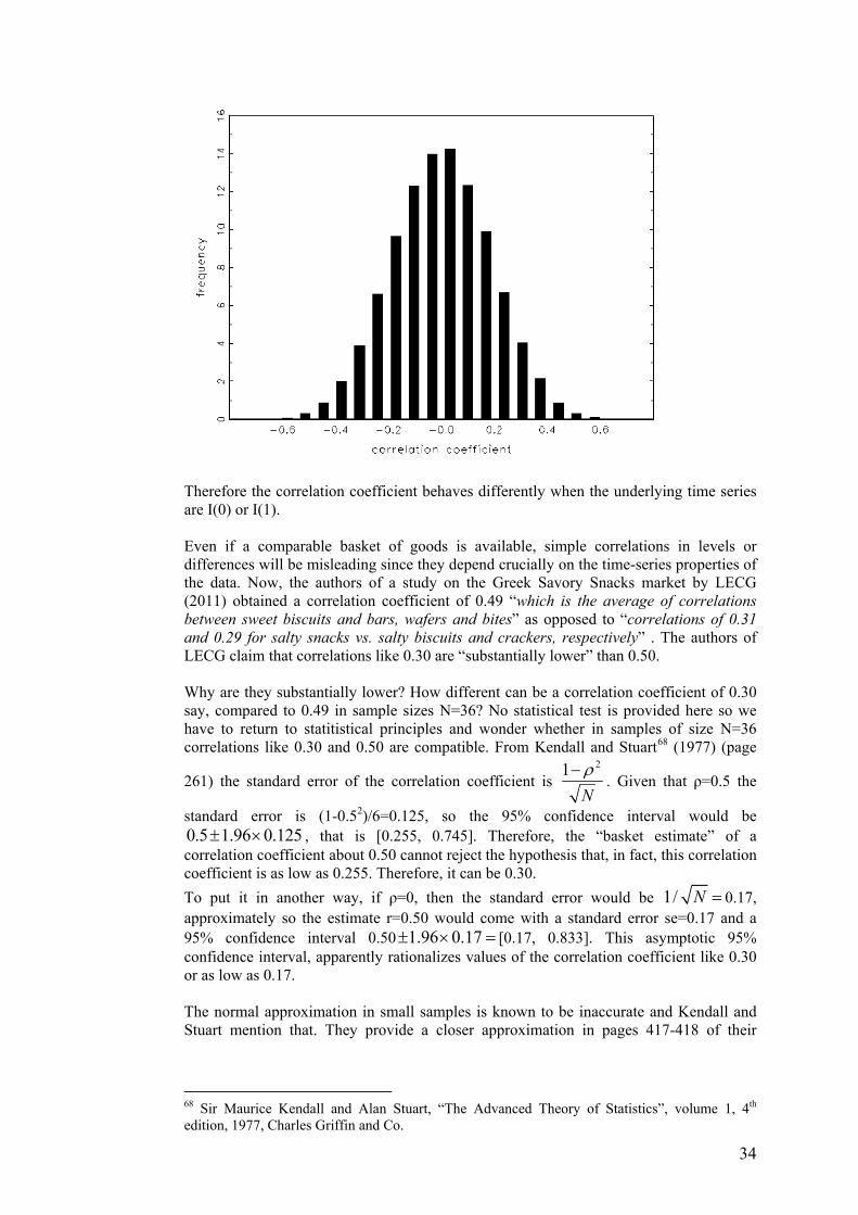
34
Therefore the correlation coefficient behaves differently when the underlying time series are I(0) or I(1). Even if a comparable basket of goods is available, simple correlations in levels or differences will be misleading since they depend crucially on the time-series properties of the data. Now, the authors of a study on the Greek Savory Snacks market by LECG (2011) obtained a correlation coefficient of 0.49 “which is the average of correlations between sweet biscuits and bars, wafers and bites” as opposed to “correlations of 0.31 and 0.29 for salty snacks vs. salty biscuits and crackers, respectively” . The authors of LECG claim that correlations like 0.30 are “substantially lower” than 0.50. Why are they substantially lower? How different can be a correlation coefficient of 0.30 say, compared to 0.49 in sample sizes N=36? No statistical test is provided here so we have to return to statitistical principles and wonder whether in samples of size N=36 correlations like 0.30 and 0.50 are compatible. From Kendall and Stuart68 (1977) (page
261) the standard error of the correlation coefficient is 21
Nρ−
. Given that ρ=0.5 the
standard error is (1-0.52)/6=0.125, so the 95% confidence interval would be 0.5 1.96 0.125± × , that is [0.255, 0.745]. Therefore, the “basket estimate” of a correlation coefficient about 0.50 cannot reject the hypothesis that, in fact, this correlation coefficient is as low as 0.255. Therefore, it can be 0.30. To put it in another way, if ρ=0, then the standard error would be 1/ N = 0.17, approximately so the estimate r=0.50 would come with a standard error se=0.17 and a 95% confidence interval 0.50 1.96 0.17± × = [0.17, 0.833]. This asymptotic 95% confidence interval, apparently rationalizes values of the correlation coefficient like 0.30 or as low as 0.17.
The normal approximation in small samples is known to be inaccurate and Kendall and Stuart mention that. They provide a closer approximation in pages 417-418 of their
68 Sir Maurice Kendall and Alan Stuart, “The Advanced Theory of Statistics”, volume 1, 4th edition, 1977, Charles Griffin and Co.
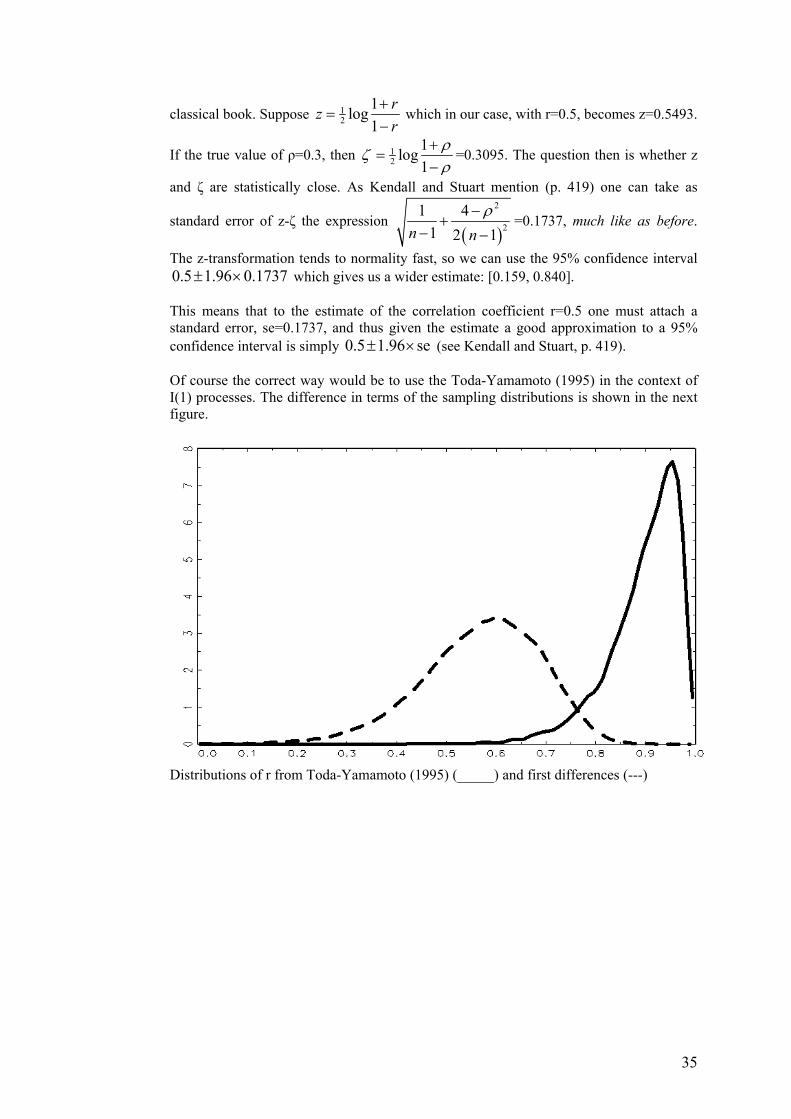
35
classical book. Suppose 12
1log1
rzr
+=
− which in our case, with r=0.5, becomes z=0.5493.
If the true value of ρ=0.3, then 12
1log1
ρζρ
+=
−=0.3095. The question then is whether z
and ζ are statistically close. As Kendall and Stuart mention (p. 419) one can take as
standard error of z-ζ the expression ( )
2
21 4
1 2 1n nρ−
+− −
=0.1737, much like as before.
The z-transformation tends to normality fast, so we can use the 95% confidence interval 0.5 1.96 0.1737± × which gives us a wider estimate: [0.159, 0.840]. This means that to the estimate of the correlation coefficient r=0.5 one must attach a standard error, se=0.1737, and thus given the estimate a good approximation to a 95% confidence interval is simply 0.5 1.96 se± × (see Kendall and Stuart, p. 419). Of course the correct way would be to use the Toda-Yamamoto (1995) in the context of I(1) processes. The difference in terms of the sampling distributions is shown in the next figure.
Distributions of r from Toda-Yamamoto (1995) (_____) and first differences (---)
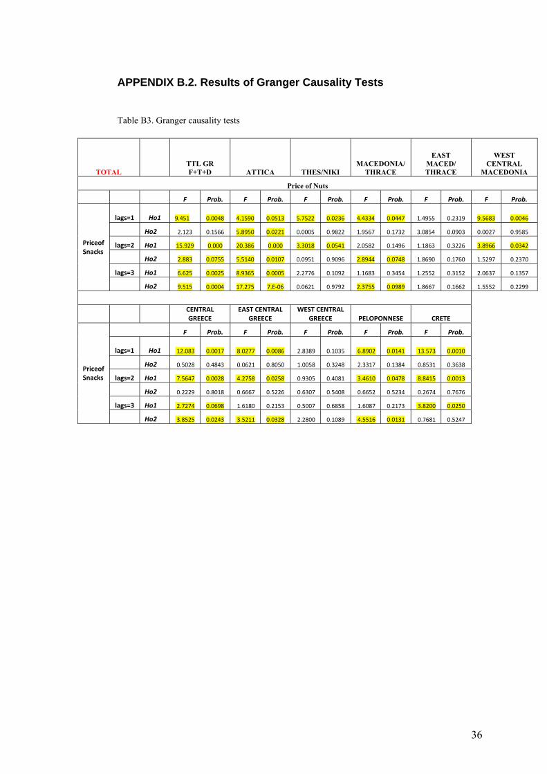
36
APPENDIX B.2. Results of Granger Causality Tests
Table B3. Granger causality tests
TOTAL TTL GR F+T+D ATTICA THES/NIKI
MACEDONIA/THRACE
EAST MACED/ THRACE
WEST CENTRAL
MACEDONIA
Price of Nuts
F Prob. F Prob. F Prob. F Prob. F Prob. F Prob.
lags=1
Ho1 9.451 0.0048 4.1590 0.0513 5.7522 0.0236 4.4334 0.0447 1.4955 0.2319 9.5683 0.0046
Ho2 2.123 0.1566 5.8950 0.0221 0.0005 0.9822 1.9567 0.1732 3.0854 0.0903 0.0027 0.9585
lags=2 Ho1 15.929 0.000 20.386 0.000 3.3018 0.0541 2.0582 0.1496 1.1863 0.3226 3.8966 0.0342
Ho2 2.883 0.0755 5.5140 0.0107 0.0951 0.9096 2.8944 0.0748 1.8690 0.1760 1.5297 0.2370
lags=3 Ho1 6.625 0.0025 8.9365 0.0005 2.2776 0.1092 1.1683 0.3454 1.2552 0.3152 2.0637 0.1357
PriceofSnacks
Ho2 9.515 0.0004 17.275 7.E‐06 0.0621 0.9792 2.3755 0.0989 1.8667 0.1662 1.5552 0.2299
CENTRAL GREECE
EAST CENTRAL GREECE
WEST CENTRAL GREECE PELOPONNESE CRETE
F Prob. F Prob. F Prob. F Prob. F Prob.
lags=1
Ho1 12.083 0.0017 8.0277 0.0086 2.8389 0.1035 6.8902 0.0141 13.573 0.0010
Ho2 0.5028 0.4843 0.0621 0.8050 1.0058 0.3248 2.3317 0.1384 0.8531 0.3638
lags=2 Ho1 7.5647 0.0028 4.2758 0.0258 0.9305 0.4081 3.4610 0.0478 8.8415 0.0013
Ho2 0.2229 0.8018 0.6667 0.5226 0.6307 0.5408 0.6652 0.5234 0.2674 0.7676
lags=3 Ho1 2.7274 0.0698 1.6180 0.2153 0.5007 0.6858 1.6087 0.2173 3.8200 0.0250
PriceofSnacks
Ho2 3.8525 0.0243 3.5211 0.0328 2.2800 0.1089 4.5516 0.0131 0.7681 0.5247
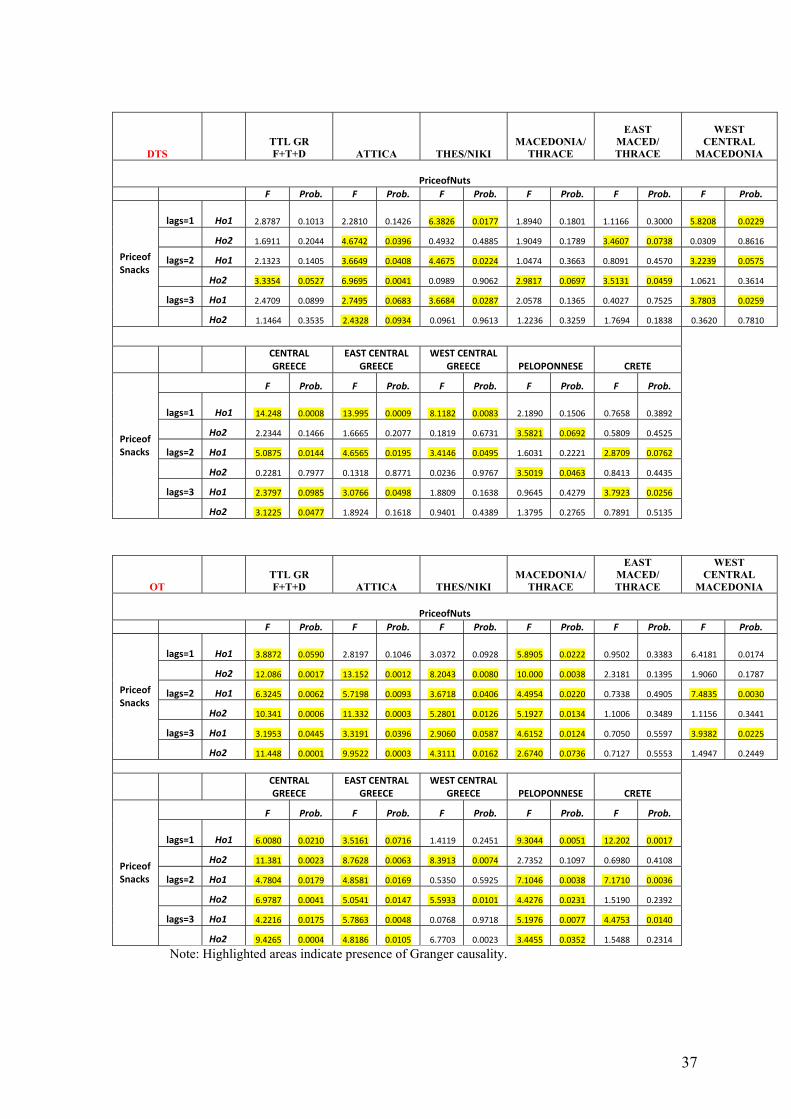
37
DTS TTL GR F+T+D ATTICA THES/NIKI
MACEDONIA/THRACE
EAST MACED/ THRACE
WEST CENTRAL
MACEDONIA
PriceofNuts F Prob. F Prob. F Prob. F Prob. F Prob. F Prob.
lags=1
Ho1 2.8787 0.1013 2.2810 0.1426 6.3826 0.0177 1.8940 0.1801 1.1166 0.3000 5.8208 0.0229
Ho2 1.6911 0.2044 4.6742 0.0396 0.4932 0.4885 1.9049 0.1789 3.4607 0.0738 0.0309 0.8616
lags=2 Ho1 2.1323 0.1405 3.6649 0.0408 4.4675 0.0224 1.0474 0.3663 0.8091 0.4570 3.2239 0.0575
Ho2 3.3354 0.0527 6.9695 0.0041 0.0989 0.9062 2.9817 0.0697 3.5131 0.0459 1.0621 0.3614
lags=3 Ho1 2.4709 0.0899 2.7495 0.0683 3.6684 0.0287 2.0578 0.1365 0.4027 0.7525 3.7803 0.0259
PriceofSnacks
Ho2 1.1464 0.3535 2.4328 0.0934 0.0961 0.9613 1.2236 0.3259 1.7694 0.1838 0.3620 0.7810
CENTRAL GREECE
EAST CENTRAL GREECE
WEST CENTRAL GREECE PELOPONNESE CRETE
F Prob. F Prob. F Prob. F Prob. F Prob.
lags=1
Ho1 14.248 0.0008 13.995 0.0009 8.1182 0.0083 2.1890 0.1506 0.7658 0.3892
Ho2 2.2344 0.1466 1.6665 0.2077 0.1819 0.6731 3.5821 0.0692 0.5809 0.4525
lags=2 Ho1 5.0875 0.0144 4.6565 0.0195 3.4146 0.0495 1.6031 0.2221 2.8709 0.0762
Ho2 0.2281 0.7977 0.1318 0.8771 0.0236 0.9767 3.5019 0.0463 0.8413 0.4435
lags=3 Ho1 2.3797 0.0985 3.0766 0.0498 1.8809 0.1638 0.9645 0.4279 3.7923 0.0256
PriceofSnacks
Ho2 3.1225 0.0477 1.8924 0.1618 0.9401 0.4389 1.3795 0.2765 0.7891 0.5135
OT TTL GR F+T+D ATTICA THES/NIKI
MACEDONIA/THRACE
EAST MACED/ THRACE
WEST CENTRAL
MACEDONIA
PriceofNuts F Prob. F Prob. F Prob. F Prob. F Prob. F Prob.
lags=1
Ho1 3.8872 0.0590 2.8197 0.1046 3.0372 0.0928 5.8905 0.0222 0.9502 0.3383 6.4181 0.0174
Ho2 12.086 0.0017 13.152 0.0012 8.2043 0.0080 10.000 0.0038 2.3181 0.1395 1.9060 0.1787
lags=2 Ho1 6.3245 0.0062 5.7198 0.0093 3.6718 0.0406 4.4954 0.0220 0.7338 0.4905 7.4835 0.0030
Ho2 10.341 0.0006 11.332 0.0003 5.2801 0.0126 5.1927 0.0134 1.1006 0.3489 1.1156 0.3441
lags=3 Ho1 3.1953 0.0445 3.3191 0.0396 2.9060 0.0587 4.6152 0.0124 0.7050 0.5597 3.9382 0.0225
PriceofSnacks
Ho2 11.448 0.0001 9.9522 0.0003 4.3111 0.0162 2.6740 0.0736 0.7127 0.5553 1.4947 0.2449
CENTRAL GREECE
EAST CENTRAL GREECE
WEST CENTRAL GREECE PELOPONNESE CRETE
F Prob. F Prob. F Prob. F Prob. F Prob.
lags=1
Ho1 6.0080 0.0210 3.5161 0.0716 1.4119 0.2451 9.3044 0.0051 12.202 0.0017
Ho2 11.381 0.0023 8.7628 0.0063 8.3913 0.0074 2.7352 0.1097 0.6980 0.4108
lags=2 Ho1 4.7804 0.0179 4.8581 0.0169 0.5350 0.5925 7.1046 0.0038 7.1710 0.0036
Ho2 6.9787 0.0041 5.0541 0.0147 5.5933 0.0101 4.4276 0.0231 1.5190 0.2392
lags=3 Ho1 4.2216 0.0175 5.7863 0.0048 0.0768 0.9718 5.1976 0.0077 4.4753 0.0140
PriceofSnacks
Ho2 9.4265 0.0004 4.8186 0.0105 6.7703 0.0023 3.4455 0.0352 1.5488 0.2314
Note: Highlighted areas indicate presence of Granger causality.
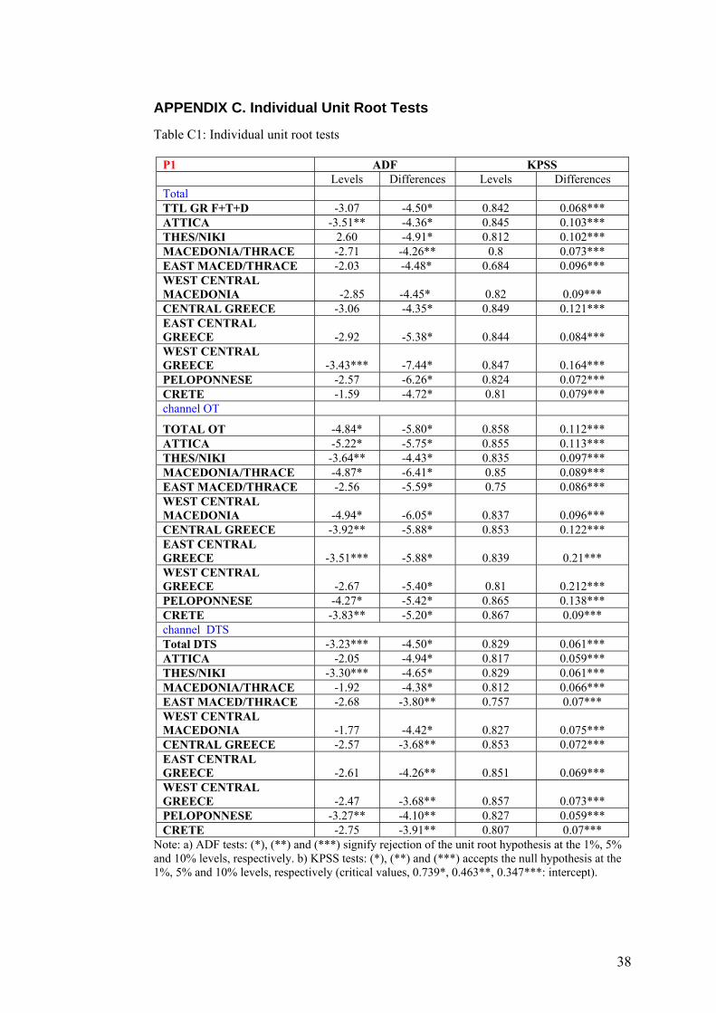
38
APPENDIX C. Individual Unit Root Tests
Table C1: Individual unit root tests
P1 ADF KPSS Levels Differences Levels Differences Total TTL GR F+T+D -3.07 -4.50* 0.842 0.068*** ATTICA -3.51** -4.36* 0.845 0.103*** THES/NIKI 2.60 -4.91* 0.812 0.102*** MACEDONIA/THRACE -2.71 -4.26** 0.8 0.073*** EAST MACED/THRACE -2.03 -4.48* 0.684 0.096*** WEST CENTRAL MACEDONIA -2.85 -4.45* 0.82 0.09*** CENTRAL GREECE -3.06 -4.35* 0.849 0.121*** EAST CENTRAL GREECE -2.92 -5.38* 0.844 0.084*** WEST CENTRAL GREECE -3.43*** -7.44* 0.847 0.164*** PELOPONNESE -2.57 -6.26* 0.824 0.072*** CRETE -1.59 -4.72* 0.81 0.079*** channel ΟΤ
TOTAL OΤ -4.84* -5.80* 0.858 0.112*** ATTICA -5.22* -5.75* 0.855 0.113*** THES/NIKI -3.64** -4.43* 0.835 0.097*** MACEDONIA/THRACE -4.87* -6.41* 0.85 0.089*** EAST MACED/THRACE -2.56 -5.59* 0.75 0.086*** WEST CENTRAL MACEDONIA -4.94* -6.05* 0.837 0.096*** CENTRAL GREECE -3.92** -5.88* 0.853 0.122*** EAST CENTRAL GREECE -3.51*** -5.88* 0.839 0.21*** WEST CENTRAL GREECE -2.67 -5.40* 0.81 0.212*** PELOPONNESE -4.27* -5.42* 0.865 0.138*** CRETE -3.83** -5.20* 0.867 0.09*** channel DTS Total DTS -3.23*** -4.50* 0.829 0.061*** ATTICA -2.05 -4.94* 0.817 0.059*** THES/NIKI -3.30*** -4.65* 0.829 0.061*** MACEDONIA/THRACE -1.92 -4.38* 0.812 0.066*** EAST MACED/THRACE -2.68 -3.80** 0.757 0.07*** WEST CENTRAL MACEDONIA -1.77 -4.42* 0.827 0.075*** CENTRAL GREECE -2.57 -3.68** 0.853 0.072*** EAST CENTRAL GREECE -2.61 -4.26** 0.851 0.069*** WEST CENTRAL GREECE -2.47 -3.68** 0.857 0.073*** PELOPONNESE -3.27** -4.10** 0.827 0.059*** CRETE -2.75 -3.91** 0.807 0.07***
Note: a) ADF tests: (*), (**) and (***) signify rejection of the unit root hypothesis at the 1%, 5% and 10% levels, respectively. b) KPSS tests: (*), (**) and (***) accepts the null hypothesis at the 1%, 5% and 10% levels, respectively (critical values, 0.739*, 0.463**, 0.347***: intercept).
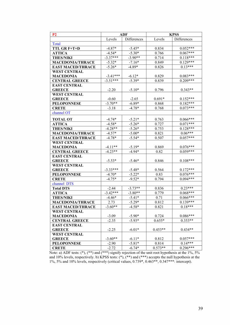
39
P2 ADF KPSS Levels Differences Levels Differences Total TTL GR F+T+D -4.87* -5.45* 0.834 0.052*** ATTICA -4.54* -5.30* 0.766 0.067*** THES/NIKI -3.37*** -3.90** 0.714 0.118*** MACEDONIA/THRACE -5.32* -7.16* 0.849 0.129*** EAST MACED/THRACE -5.26* -4.89* 0.826 0.13*** WEST CENTRAL MACEDONIA -3.41*** -6.12* 0.829 0.083*** CENTRAL GREECE -3.51*** -5.39* 0.839 0.209*** EAST CENTRAL GREECE -2.20 -5.10* 0.796 0.343** WEST CENTRAL GREECE -0.60 -2.65 0.691* 0.152*** PELOPONNESE -3.70** -6.89* 0.868 0.182*** CRETE -3.18 -4.78* 0.768 0.073*** channel ΟΤ
TOTAL OΤ -4.74* -5.21* 0.763 0.066*** ATTICA -4.58* -5.26* 0.727 0.071*** THES/NIKI -4.28** -5.26* 0.753 0.128*** MACEDONIA/THRACE -4.57* -5.00* 0.821 0.06*** EAST MACED/THRACE -4.78* -5.54* 0.507 0.057*** WEST CENTRAL MACEDONIA -4.11** -5.19* 0.869 0.076*** CENTRAL GREECE -4.23** -4.94* 0.82 0.059*** EAST CENTRAL GREECE -5.53* -5.46* 0.846 0.108*** WEST CENTRAL GREECE -3.33*** -5.48* 0.564 0.172*** PELOPONNESE -4.70* -5.22* 0.83 0.076*** CRETE -4.75* -9.52* 0.794 0.094*** channel DTS Total DTS -2.44 -3.73** 0.836 0.23*** ATTICA -3.42*** -3.80** 0.779 0.068*** THES/NIKI -4.46* -5.41* 0.71 0.066*** MACEDONIA/THRACE 2.73 -5.29* 0.812 0.139*** EAST MACED/THRACE -3.60** -4.58* 0.821 0.18*** WEST CENTRAL MACEDONIA -3.09 -5.90* 0.724 0.086*** CENTRAL GREECE -2.35 -5.93* 0.655* 0.353** EAST CENTRAL GREECE -2.25 -6.01* 0.453** 0.434** WEST CENTRAL GREECE -3.60** -6.11* 0.812 0.057*** PELOPONNESE -2.90 -5.81* 0.814 0.14*** CRETE -2.72 -6.74* 0.573** 0.296***
Note: a) ADF tests: (*), (**) and (***) signify rejection of the unit root hypothesis at the 1%, 5% and 10% levels, respectively. b) KPSS tests: (*), (**) and (***) accepts the null hypothesis at the 1%, 5% and 10% levels, respectively (critical values, 0.739*, 0.463**, 0.347***: intercept).
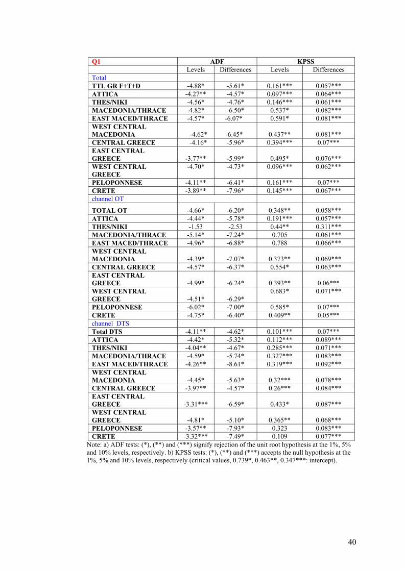
40
Q1 ADF KPSS Levels Differences Levels Differences Total TTL GR F+T+D -4.88* -5.61* 0.161*** 0.057*** ATTICA -4.27** -4.57* 0.097*** 0.064*** THES/NIKI -4.56* -4.76* 0.146*** 0.061*** MACEDONIA/THRACE -4.82* -6.50* 0.537* 0.082*** EAST MACED/THRACE -4.57* -6.07* 0.591* 0.081*** WEST CENTRAL MACEDONIA -4.62* -6.45* 0.437** 0.081*** CENTRAL GREECE -4.16* -5.96* 0.394*** 0.07*** EAST CENTRAL GREECE -3.77** -5.99* 0.495* 0.076*** WEST CENTRAL GREECE
-4.70* -4.73* 0.096*** 0.062***
PELOPONNESE -4.11** -6.41* 0.161*** 0.07*** CRETE -3.89** -7.96* 0.145*** 0.067*** channel ΟΤ
TOTAL OΤ -4.66* -6.20* 0.348** 0.058*** ATTICA -4.44* -5.78* 0.191*** 0.057*** THES/NIKI -1.53 -2.53 0.44** 0.311*** MACEDONIA/THRACE -5.14* -7.24* 0.705 0.061*** EAST MACED/THRACE -4.96* -6.88* 0.788 0.066*** WEST CENTRAL MACEDONIA -4.39* -7.07* 0.373** 0.069*** CENTRAL GREECE -4.57* -6.37* 0.554* 0.063*** EAST CENTRAL GREECE -4.99* -6.24* 0.393** 0.06*** WEST CENTRAL GREECE -4.51* -6.29*
0.683* 0.071***
PELOPONNESE -6.02* -7.00* 0.585* 0.07*** CRETE -4.75* -6.40* 0.409** 0.05*** channel DTS Total DTS -4.11** -4.62* 0.101*** 0.07*** ATTICA -4.42* -5.32* 0.112*** 0.089*** THES/NIKI -4.04** -4.67* 0.285*** 0.071*** MACEDONIA/THRACE -4.59* -5.74* 0.327*** 0.083*** EAST MACED/THRACE -4.26** -8.61* 0.319*** 0.092*** WEST CENTRAL MACEDONIA -4.45* -5.63* 0.32*** 0.078*** CENTRAL GREECE -3.97** -4.57* 0.26*** 0.084*** EAST CENTRAL GREECE -3.31*** -6.59* 0.433* 0.087*** WEST CENTRAL GREECE -4.81* -5.10* 0.365** 0.068*** PELOPONNESE -3.57** -7.93* 0.323 0.083*** CRETE -3.32*** -7.49* 0.109 0.077***
Note: a) ADF tests: (*), (**) and (***) signify rejection of the unit root hypothesis at the 1%, 5% and 10% levels, respectively. b) KPSS tests: (*), (**) and (***) accepts the null hypothesis at the 1%, 5% and 10% levels, respectively (critical values, 0.739*, 0.463**, 0.347***: intercept).
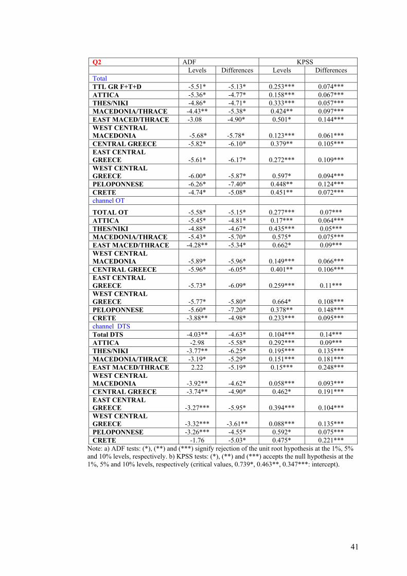
41
Q2 ADF KPSS Levels Differences Levels Differences Total TTL GR F+T+D -5.51* -5.13* 0.253*** 0.074*** ATTICA -5.36* -4.77* 0.158*** 0.067*** THES/NIKI -4.86* -4.71* 0.333*** 0.057*** MACEDONIA/THRACE -4.43** -5.38* 0.424** 0.097*** EAST MACED/THRACE -3.08 -4.90* 0.501* 0.144*** WEST CENTRAL MACEDONIA -5.68* -5.78* 0.123*** 0.061*** CENTRAL GREECE -5.82* -6.10* 0.379** 0.105*** EAST CENTRAL GREECE -5.61* -6.17* 0.272*** 0.109*** WEST CENTRAL GREECE -6.00* -5.87* 0.597* 0.094*** PELOPONNESE -6.26* -7.40* 0.448** 0.124*** CRETE -4.74* -5.08* 0.451** 0.072*** channel ΟΤ
TOTAL OΤ -5.58* -5.15* 0.277*** 0.07*** ATTICA -5.45* -4.81* 0.17*** 0.064*** THES/NIKI -4.88* -4.67* 0.435*** 0.05*** MACEDONIA/THRACE -5.43* -5.70* 0.575* 0.075*** EAST MACED/THRACE -4.28** -5.34* 0.662* 0.09*** WEST CENTRAL MACEDONIA -5.89* -5.96* 0.149*** 0.066*** CENTRAL GREECE -5.96* -6.05* 0.401** 0.106*** EAST CENTRAL GREECE -5.73* -6.09* 0.259*** 0.11*** WEST CENTRAL GREECE -5.77* -5.80* 0.664* 0.108*** PELOPONNESE -5.60* -7.20* 0.378** 0.148*** CRETE -3.88** -4.98* 0.233*** 0.095*** channel DTS Total DTS -4.03** -4.63* 0.104*** 0.14*** ATTICA -2.98 -5.58* 0.292*** 0.09*** THES/NIKI -3.77** -6.25* 0.195*** 0.135*** MACEDONIA/THRACE -3.19* -5.29* 0.151*** 0.181*** EAST MACED/THRACE 2.22 -5.19* 0.15*** 0.248*** WEST CENTRAL MACEDONIA -3.92** -4.62* 0.058*** 0.093*** CENTRAL GREECE -3.74** -4.90* 0.462* 0.191*** EAST CENTRAL GREECE -3.27*** -5.95* 0.394*** 0.104*** WEST CENTRAL GREECE -3.32*** -3.61** 0.088*** 0.135*** PELOPONNESE -3.26*** -4.55* 0.592* 0.075*** CRETE -1.76 -5.03* 0.475* 0.221***
Note: a) ADF tests: (*), (**) and (***) signify rejection of the unit root hypothesis at the 1%, 5% and 10% levels, respectively. b) KPSS tests: (*), (**) and (***) accepts the null hypothesis at the 1%, 5% and 10% levels, respectively (critical values, 0.739*, 0.463**, 0.347***: intercept).

42
Log (P1) ADF KPSS Levels Differences Levels Differences Total TTL GR F+T+D -3.02 -4.38* 0.84 0.50*** ATTICA -3.43*** -4.61* 0.84 0.112*** THES/NIKI -2.55 -4.82* 0.81 0.104*** MACEDONIA/THRACE -2.66 -4.21** 0.801 0.073*** EAST MACED/THRACE -1.98 -4.56* 0.678 0.093*** WEST CENTRAL MACEDONIA -2.79 4.47* 0.822 0.093*** CENTRAL GREECE -3.13 -7.31* 0.851 0.106*** EAST CENTRAL GREECE -2.99 -6.3* 0.845 0.075*** WEST CENTRAL GREECE -3.47*** -7.35* 0.848 0.149*** PELOPONNESE -2.62 -6.29* 0.824 0.072*** CRETE -1.71 -4.76* 0.81 0.079*** channel ΟΤ
TOTAL OΤ -4.85* -5.81* 0.858 0.112*** ATTICA -5.06* -5.67* 0.855 0.113*** THES/NIKI -3.66** -5.4* 0.835 0.097*** MACEDONIA/THRACE -5.05* -6.55* 0.85 0.089*** EAST MACED/THRACE -2.56 -5.58* 0.75 0.086*** WEST CENTRAL MACEDONIA -4.64* -6.19* 0.837 0.096*** CENTRAL GREECE -3.87** -5.88* 0.853 0.122*** EAST CENTRAL GREECE
-3.3*** -5.84* 0.839 0.210***
WEST CENTRAL GREECE
-2.77 -5.47* 0.81 0.212***
PELOPONNESE -4.32* -5.5* 0.865 0.138*** CRETE -3.81* -5.32* 0.867 0.092*** channel DTS Total DTS -3.22 -4.45* 0.829 0.0617*** ATTICA -3.44*** -4.87* 0.817 0.59* THES/NIKI -3.3*** -4.58* 0.829 0.0617*** MACEDONIA/THRACE -1.93 -4.32* 0.812 0.066*** EAST MACED/THRACE -2.65 -3.83** 0.757 0.708 WEST CENTRAL MACEDONIA
-1.77 -4.39* 0.827 0.0756***
CENTRAL GREECE -2.62 -3.72** 0.853 0.0726*** EAST CENTRAL GREECE
-2.67 -4.34* 0.851 0.0693***
WEST CENTRAL GREECE
-2.51 -3.62** 0.857 0.731
PELOPONNESE -3.27*** -4.13** 0.827 0.0592*** CRETE -2.76 -3.91** 0.807 0.0705***
Note: a) ADF tests: (*), (**) and (***) signify rejection of the unit root hypothesis at the 1%, 5% and 10% levels, respectively. b) KPSS tests: (*), (**) and (***) accepts the null hypothesis at the 1%, 5% and 10% levels, respectively (critical values, 0.739*, 0.463**, 0.347***: intercept).
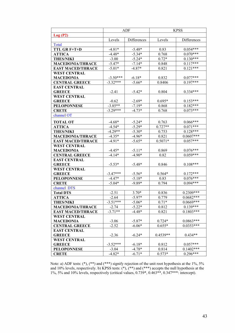
43
Note: a) ADF tests: (*), (**) and (***) signify rejection of the unit root hypothesis at the 1%, 5% and 10% levels, respectively. b) KPSS tests: (*), (**) and (***) accepts the null hypothesis at the 1%, 5% and 10% levels, respectively (critical values, 0.739*, 0.463**, 0.347***: intercept).
ADF KPSS Log (P2) Levels Differences Levels Differences Total TTL GR F+T+D -4.81* -5.48* 0.83 0.054*** ATTICA -4.48* -5.34* 0.768 0.070*** THES/NIKI -3.00 -5.24* 0.72* 0.130*** MACEDONIA/THRACE -5.47* -7.14* 0.848 0.117*** EAST MACED/THRACE -5.01* -4.87* 0.821 0.121*** WEST CENTRAL MACEDONIA -3.50*** -6.18* 0.832 0.077*** CENTRAL GREECE -3.32*** -5.66* 0.8406 0.197*** EAST CENTRAL GREECE -2.41 -5.42* 0.804 0.334*** WEST CENTRAL GREECE -0.62 -2.69* 0.695* 0.153*** PELOPONNESE -3.85** -7.19* 0.868 0.182*** CRETE -3.29*** -4.73* 0.768 0.073*** channel ΟΤ
TOTAL OΤ -4.68* -5.24* 0.763 0.066*** ATTICA -4.54* -5.29* 0.727** 0.071*** THES/NIKI -4.29** -5.30* 0.753 0.128*** MACEDONIA/THRACE -4.35* -4.96* 0.821 0.0607*** EAST MACED/THRACE -4.91* -5.65* 0.5071* 0.057*** WEST CENTRAL MACEDONIA -4.45* -5.11* 0.869 0.076*** CENTRAL GREECE -4.14* -4.90* 0.82 0.059*** EAST CENTRAL GREECE -5.53* -5.48* 0.846 0.108*** WEST CENTRAL GREECE -3.47*** -5.56* 0.564* 0.172*** PELOPONNESE -4.47* -5.18* 0.83 0.076*** CRETE -5.04* -9.89* 0.794 0.094*** channel DTS Total DTS -2.51 3.70* 0.836 0.2309*** ATTICA -2.64 -5.97* 0.779 0.0682*** THES/NIKI -3.51*** -5.06* 0.71* 0.0669*** MACEDONIA/THRACE -2.74 -5.22* 0.812 0.139*** EAST MACED/THRACE -3.71** -4.48* 0.821 0.1803*** WEST CENTRAL MACEDONIA -3.06 -5.87* 0.724* 0.0863*** CENTRAL GREECE -2.52 -6.06* 0.655* 0.0353*** EAST CENTRAL GREECE -2.36 -6.24* 0.4539** 0.434** WEST CENTRAL GREECE -3.52*** -6.18* 0.812 0.057*** PELOPONNESE -3.04 -4.78* 0.814 0.1402*** CRETE -4.82* -6.71* 0.573* 0.296***
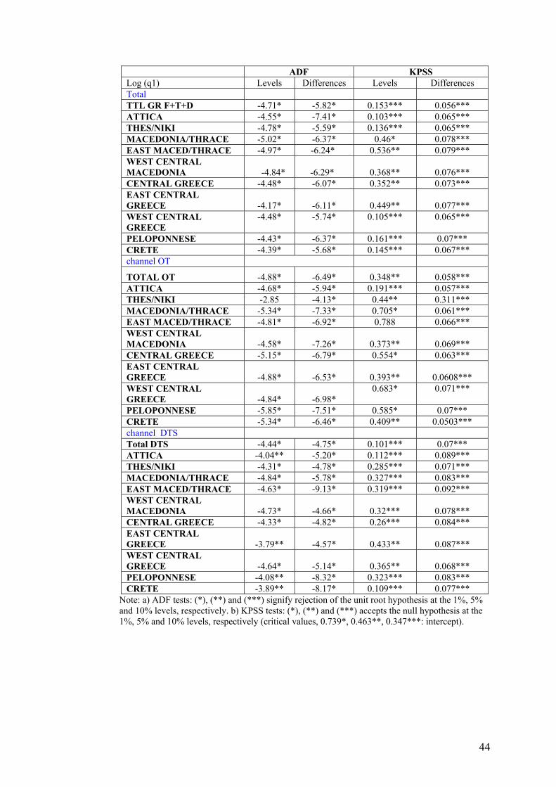
44
ADF KPSS Log (q1) Levels Differences Levels Differences Total TTL GR F+T+D -4.71* -5.82* 0.153*** 0.056*** ATTICA -4.55* -7.41* 0.103*** 0.065*** THES/NIKI -4.78* -5.59* 0.136*** 0.065*** MACEDONIA/THRACE -5.02* -6.37* 0.46* 0.078*** EAST MACED/THRACE -4.97* -6.24* 0.536** 0.079*** WEST CENTRAL MACEDONIA -4.84* -6.29* 0.368** 0.076*** CENTRAL GREECE -4.48* -6.07* 0.352** 0.073*** EAST CENTRAL GREECE -4.17* -6.11* 0.449** 0.077*** WEST CENTRAL GREECE
-4.48* -5.74* 0.105*** 0.065***
PELOPONNESE -4.43* -6.37* 0.161*** 0.07*** CRETE -4.39* -5.68* 0.145*** 0.067*** channel ΟΤ
TOTAL OΤ -4.88* -6.49* 0.348** 0.058*** ATTICA -4.68* -5.94* 0.191*** 0.057*** THES/NIKI -2.85 -4.13* 0.44** 0.311*** MACEDONIA/THRACE -5.34* -7.33* 0.705* 0.061*** EAST MACED/THRACE -4.81* -6.92* 0.788 0.066*** WEST CENTRAL MACEDONIA -4.58* -7.26* 0.373** 0.069*** CENTRAL GREECE -5.15* -6.79* 0.554* 0.063*** EAST CENTRAL GREECE -4.88* -6.53* 0.393** 0.0608*** WEST CENTRAL GREECE -4.84* -6.98*
0.683* 0.071***
PELOPONNESE -5.85* -7.51* 0.585* 0.07*** CRETE -5.34* -6.46* 0.409** 0.0503*** channel DTS Total DTS -4.44* -4.75* 0.101*** 0.07*** ATTICA -4.04** -5.20* 0.112*** 0.089*** THES/NIKI -4.31* -4.78* 0.285*** 0.071*** MACEDONIA/THRACE -4.84* -5.78* 0.327*** 0.083*** EAST MACED/THRACE -4.63* -9.13* 0.319*** 0.092*** WEST CENTRAL MACEDONIA -4.73* -4.66* 0.32*** 0.078*** CENTRAL GREECE -4.33* -4.82* 0.26*** 0.084*** EAST CENTRAL GREECE -3.79** -4.57* 0.433** 0.087*** WEST CENTRAL GREECE -4.64* -5.14* 0.365** 0.068*** PELOPONNESE -4.08** -8.32* 0.323*** 0.083*** CRETE -3.89** -8.17* 0.109*** 0.077***
Note: a) ADF tests: (*), (**) and (***) signify rejection of the unit root hypothesis at the 1%, 5% and 10% levels, respectively. b) KPSS tests: (*), (**) and (***) accepts the null hypothesis at the 1%, 5% and 10% levels, respectively (critical values, 0.739*, 0.463**, 0.347***: intercept).
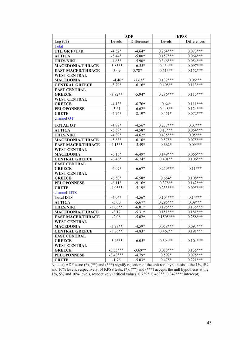
45
ADF KPSS Log (q2) Levels Differences Levels Differences Total TTL GR F+T+D -4.32* -4.64* 0.264*** 0.073*** ATTICA -5.44* -5.00* 0.157*** 0.064*** THES/NIKI -4.65* -5.90* 0.346*** 0.054*** MACEDONIA/THRACE -3.85** -6.55* 0.434** 0.097*** EAST MACED/THRACE -3.09 -5.78* 0.513** 0.152*** WEST CENTRAL MACEDONIA -4.46* -7.63* 0.132*** 0.06*** CENTRAL GREECE -3.79* -6.16* 0.408** 0.113*** EAST CENTRAL GREECE -3.82** -5.94* 0.286*** 0.115*** WEST CENTRAL GREECE -4.13* -6.76* 0.64* 0.111*** PELOPONNESE -3.61 -6.62* 0.448** 0.124*** CRETE -4.76* -8.19* 0.451* 0.072*** channel ΟΤ
TOTAL OΤ -4.98* -4.56* 0.277*** 0.07*** ATTICA -5.39* -4.58* 0.17*** 0.064*** THES/NIKI -4.89* -4.62* 0.435*** 0.05*** MACEDONIA/THRACE -5.83* -6.10* 0.575* 0.075*** EAST MACED/THRACE -4.13** -5.49* 0.662* 0.09*** WEST CENTRAL MACEDONIA -6.15* -6.49* 0.149*** 0.066*** CENTRAL GREECE -6.46* -6.74* 0.401** 0.106*** EAST CENTRAL GREECE -6.07* -6.67* 0.259*** 0.11*** WEST CENTRAL GREECE -6.50* -6.58* 0.664* 0.108*** PELOPONNESE -6.11* -9.16* 0.378** 0.142*** CRETE -4.05** -5.19* 0.233*** 0.095*** channel DTS Total DTS -4.04* -4.56* 0.104*** 0.14*** ATTICA -3.00 -5.67* 0.295*** 0.09*** THES/NIKI -3.63** -6.01* 0.195*** 0.135*** MACEDONIA/THRACE -3.17 -5.31* 0.151*** 0.181*** EAST MACED/THRACE -2.08 -5.02* 0.1505*** 0.258*** WEST CENTRAL MACEDONIA -3.97** -4.59* 0.058*** 0.093*** CENTRAL GREECE -3.86** -4.83* 0.462** 0.191*** EAST CENTRAL GREECE -3.46** -6.05* 0.394** 0.104*** WEST CENTRAL GREECE -3.33*** -3.69** 0.088*** 0.135*** PELOPONNESE -3.48*** -4.79* 0.592* 0.075*** CRETE -1.76 -5.03* 0.475* 0.221***
Note: a) ADF tests: (*), (**) and (***) signify rejection of the unit root hypothesis at the 1%, 5% and 10% levels, respectively. b) KPSS tests: (*), (**) and (***) accepts the null hypothesis at the 1%, 5% and 10% levels, respectively (critical values, 0.739*, 0.463**, 0.347***: intercept).
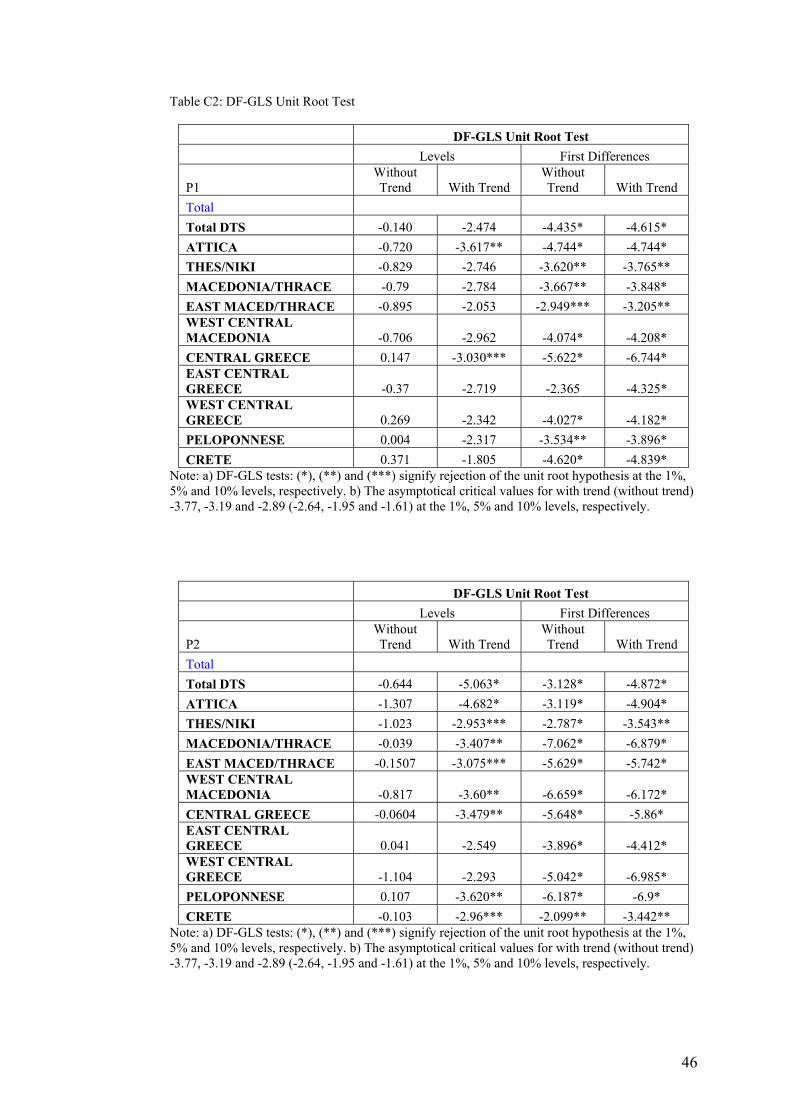
46
Table C2: DF-GLS Unit Root Test
DF-GLS Unit Root Test Levels First Differences
P1 Without Trend With Trend
Without Trend With Trend
Total Total DTS -0.140 -2.474 -4.435* -4.615* ATTICA -0.720 -3.617** -4.744* -4.744* THES/NIKI -0.829 -2.746 -3.620** -3.765** MACEDONIA/THRACE -0.79 -2.784 -3.667** -3.848* EAST MACED/THRACE -0.895 -2.053 -2.949*** -3.205** WEST CENTRAL MACEDONIA -0.706 -2.962 -4.074* -4.208* CENTRAL GREECE 0.147 -3.030*** -5.622* -6.744* EAST CENTRAL GREECE -0.37 -2.719 -2.365 -4.325* WEST CENTRAL GREECE 0.269 -2.342 -4.027* -4.182* PELOPONNESE 0.004 -2.317 -3.534** -3.896* CRETE 0.371 -1.805 -4.620* -4.839*
Note: a) DF-GLS tests: (*), (**) and (***) signify rejection of the unit root hypothesis at the 1%, 5% and 10% levels, respectively. b) The asymptotical critical values for with trend (without trend) -3.77, -3.19 and -2.89 (-2.64, -1.95 and -1.61) at the 1%, 5% and 10% levels, respectively.
DF-GLS Unit Root Test Levels First Differences
P2 Without Trend With Trend
Without Trend With Trend
Total Total DTS -0.644 -5.063* -3.128* -4.872* ATTICA -1.307 -4.682* -3.119* -4.904* THES/NIKI -1.023 -2.953*** -2.787* -3.543** MACEDONIA/THRACE -0.039 -3.407** -7.062* -6.879* EAST MACED/THRACE -0.1507 -3.075*** -5.629* -5.742* WEST CENTRAL MACEDONIA -0.817 -3.60** -6.659* -6.172* CENTRAL GREECE -0.0604 -3.479** -5.648* -5.86* EAST CENTRAL GREECE 0.041 -2.549 -3.896* -4.412* WEST CENTRAL GREECE -1.104 -2.293 -5.042* -6.985* PELOPONNESE 0.107 -3.620** -6.187* -6.9* CRETE -0.103 -2.96*** -2.099** -3.442**
Note: a) DF-GLS tests: (*), (**) and (***) signify rejection of the unit root hypothesis at the 1%, 5% and 10% levels, respectively. b) The asymptotical critical values for with trend (without trend) -3.77, -3.19 and -2.89 (-2.64, -1.95 and -1.61) at the 1%, 5% and 10% levels, respectively.
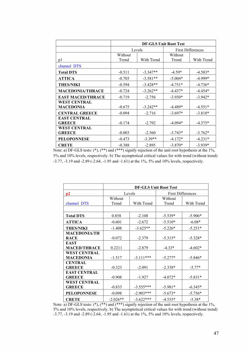
47
DF-GLS Unit Root Test Levels First Differences
p1 Without Trend With Trend
Without Trend With Trend
channel DTS Total DTS -0.511 -3.347** -4.59* -4.583* ATTICA -0.703 -3.581** -5.004* -4.999* THES/NIKI -0.594 -3.428** -4.751* -4.736* MACEDONIA/THRACE -0.724 -3.262** -4.437* -4.454* EAST MACED/THRACE -0.719 -2.756 -3.930* -3.942* WEST CENTRAL MACEDONIA -0.675 -3.242** -4.489* -4.551* CENTRAL GREECE -0.094 -2.716 -3.697* -3.818* EAST CENTRAL GREECE -0.174 -2.792 -4.094* -4.375* WEST CENTRAL GREECE -0.003 -2.560 -3.743* -3.762* PELOPONNESE -0.473 -3.39** -4.172* -4.231* CRETE -0.388 -2.895 -3.870* -3.939*
Note: a) DF-GLS tests: (*), (**) and (***) signify rejection of the unit root hypothesis at the 1%, 5% and 10% levels, respectively. b) The asymptotical critical values for with trend (without trend) -3.77, -3.19 and -2.89 (-2.64, -1.95 and -1.61) at the 1%, 5% and 10% levels, respectively.
DF-GLS Unit Root Test p2 Levels First Differences
channel DTS Without Trend With Trend
Without Trend With Trend
Total DTS 0.858 -2.108 -5.539* -5.906* ATTICA -0.601 -2.672 -5.510* -6.08* THES/NIKI -1.408 -3.625** -5.226* -5.251* MACEDONIA/THRACE -0.072 -2.379 -5.315* -5.328* EAST MACED/THRACE 0.2211 -2.879 -4.33* -4.602* WEST CENTRAL MACEDONIA -1.517 -3.111*** -5.277* -5.846* CENTRAL GREECE -0.323 -2.091 -2.338* -5.77* EAST CENTRAL GREECE -0.908 -1.927 -4.072* -5.831* WEST CENTRAL GREECE -0.833 -3.555*** -5.981* -6.345* PELOPONNESE -0.098 -2.903*** -5.673* -5.756* CRETE -2.026** -3.622*** -4.555* -5.38*
Note: a) DF-GLS tests: (*), (**) and (***) signify rejection of the unit root hypothesis at the 1%, 5% and 10% levels, respectively. b) The asymptotical critical values for with trend (without trend) -3.77, -3.19 and -2.89 (-2.64, -1.95 and -1.61) at the 1%, 5% and 10% levels, respectively.
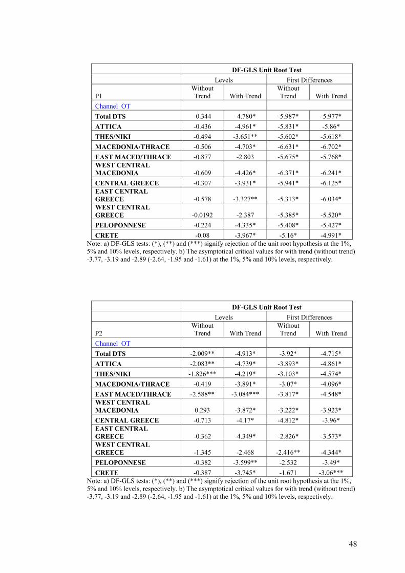
48
DF-GLS Unit Root Test Levels First Differences
P1 Without Trend With Trend
Without Trend With Trend
Channel OT Total DTS -0.344 -4.780* -5.987* -5.977* ATTICA -0.436 -4.961* -5.831* -5.86* THES/NIKI -0.494 -3.651** -5.602* -5.618* MACEDONIA/THRACE -0.506 -4.703* -6.631* -6.702* EAST MACED/THRACE -0.877 -2.803 -5.675* -5.768* WEST CENTRAL MACEDONIA -0.609 -4.426* -6.371* -6.241* CENTRAL GREECE -0.307 -3.931* -5.941* -6.125* EAST CENTRAL GREECE -0.578 -3.327** -5.313* -6.034* WEST CENTRAL GREECE -0.0192 -2.387 -5.385* -5.520* PELOPONNESE -0.224 -4.335* -5.408* -5.427* CRETE -0.08 -3.967* -5.16* -4.991*
Note: a) DF-GLS tests: (*), (**) and (***) signify rejection of the unit root hypothesis at the 1%, 5% and 10% levels, respectively. b) The asymptotical critical values for with trend (without trend) -3.77, -3.19 and -2.89 (-2.64, -1.95 and -1.61) at the 1%, 5% and 10% levels, respectively.
DF-GLS Unit Root Test Levels First Differences
P2 Without Trend With Trend
Without Trend With Trend
Channel OT Total DTS -2.009** -4.913* -3.92* -4.715* ATTICA -2.083** -4.739* -3.893* -4.861* THES/NIKI -1.826*** -4.219* -3.103* -4.574* MACEDONIA/THRACE -0.419 -3.891* -3.07* -4.096* EAST MACED/THRACE -2.588** -3.084*** -3.817* -4.548* WEST CENTRAL MACEDONIA 0.293 -3.872* -3.222* -3.923* CENTRAL GREECE -0.713 -4.17* -4.812* -3.96* EAST CENTRAL GREECE -0.362 -4.349* -2.826* -3.573* WEST CENTRAL GREECE -1.345 -2.468 -2.416** -4.344* PELOPONNESE -0.382 -3.599** -2.532 -3.49* CRETE -0.387 -3.745* -1.671 -3.06***
Note: a) DF-GLS tests: (*), (**) and (***) signify rejection of the unit root hypothesis at the 1%, 5% and 10% levels, respectively. b) The asymptotical critical values for with trend (without trend) -3.77, -3.19 and -2.89 (-2.64, -1.95 and -1.61) at the 1%, 5% and 10% levels, respectively.
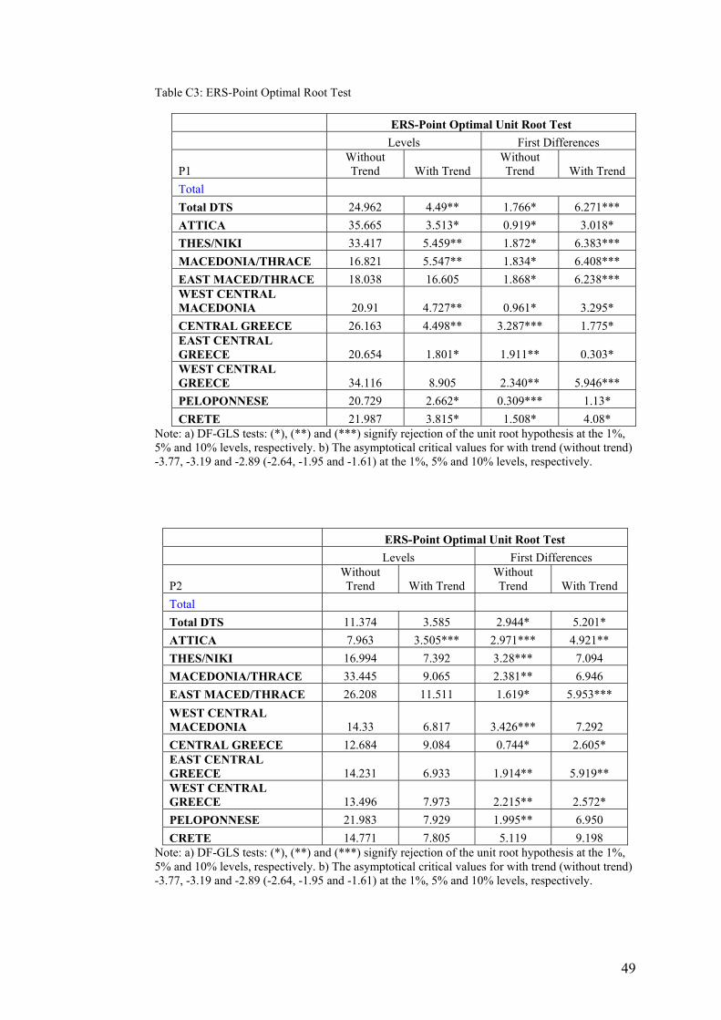
49
Table C3: ERS-Point Optimal Root Test
ERS-Point Optimal Unit Root Test Levels First Differences
P1 Without Trend With Trend
Without Trend With Trend
Total Total DTS 24.962 4.49** 1.766* 6.271*** ATTICA 35.665 3.513* 0.919* 3.018* THES/NIKI 33.417 5.459** 1.872* 6.383*** MACEDONIA/THRACE 16.821 5.547** 1.834* 6.408*** EAST MACED/THRACE 18.038 16.605 1.868* 6.238*** WEST CENTRAL MACEDONIA 20.91 4.727** 0.961* 3.295* CENTRAL GREECE 26.163 4.498** 3.287*** 1.775* EAST CENTRAL GREECE 20.654 1.801* 1.911** 0.303* WEST CENTRAL GREECE 34.116 8.905 2.340** 5.946*** PELOPONNESE 20.729 2.662* 0.309*** 1.13* CRETE 21.987 3.815* 1.508* 4.08*
Note: a) DF-GLS tests: (*), (**) and (***) signify rejection of the unit root hypothesis at the 1%, 5% and 10% levels, respectively. b) The asymptotical critical values for with trend (without trend) -3.77, -3.19 and -2.89 (-2.64, -1.95 and -1.61) at the 1%, 5% and 10% levels, respectively.
ERS-Point Optimal Unit Root Test Levels First Differences
P2 Without Trend With Trend
Without Trend With Trend
Total Total DTS 11.374 3.585 2.944* 5.201* ATTICA 7.963 3.505*** 2.971*** 4.921** THES/NIKI 16.994 7.392 3.28*** 7.094 MACEDONIA/THRACE 33.445 9.065 2.381** 6.946 EAST MACED/THRACE 26.208 11.511 1.619* 5.953*** WEST CENTRAL MACEDONIA 14.33 6.817 3.426*** 7.292 CENTRAL GREECE 12.684 9.084 0.744* 2.605* EAST CENTRAL GREECE 14.231 6.933 1.914** 5.919** WEST CENTRAL GREECE 13.496 7.973 2.215** 2.572* PELOPONNESE 21.983 7.929 1.995** 6.950 CRETE 14.771 7.805 5.119 9.198
Note: a) DF-GLS tests: (*), (**) and (***) signify rejection of the unit root hypothesis at the 1%, 5% and 10% levels, respectively. b) The asymptotical critical values for with trend (without trend) -3.77, -3.19 and -2.89 (-2.64, -1.95 and -1.61) at the 1%, 5% and 10% levels, respectively.
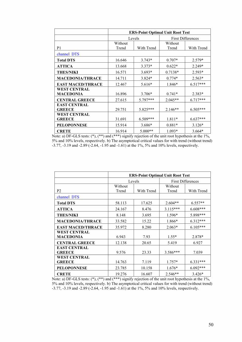
50
ERS-Point Optimal Unit Root Test Levels First Differences
P1 Without Trend With Trend
Without Trend With Trend
channel DTS Total DTS 16.646 3.743* 0.707* 2.579* ATTICA 13.668 3.373* 0.622* 2.249* THES/NIKI 16.571 3.693* 0.7138* 2.593* MACEDONIA/THRACE 14.711 3.824* 0.774* 2.563* EAST MACED/THRACE 12.467 5.616* 1.846* 6.517*** WEST CENTRAL MACEDONIA 16.896 3.706* 0.741* 2.383* CENTRAL GREECE 27.615 5.797*** 2.045** 6.717*** EAST CENTRAL GREECE 29.751 5.825*** 2.146** 6.505*** WEST CENTRAL GREECE 31.691 6.509*** 1.811* 6.637*** PELOPONNESE 15.914 3.686* 0.881* 3.126* CRETE 16.914 5.000** 1.093* 3.664*
Note: a) DF-GLS tests: (*), (**) and (***) signify rejection of the unit root hypothesis at the 1%, 5% and 10% levels, respectively. b) The asymptotical critical values for with trend (without trend) -3.77, -3.19 and -2.89 (-2.64, -1.95 and -1.61) at the 1%, 5% and 10% levels, respectively.
ERS-Point Optimal Unit Root Test Levels First Differences
P2 Without Trend With Trend
Without Trend With Trend
channel DTS Total DTS 58.113 17.625 2.604** 6.557** ATTICA 24.167 8.476 3.115*** 6.608*** THES/NIKI 8.148 3.695 1.596* 5.898*** MACEDONIA/THRACE 33.582 15.22 1.866* 6.312*** EAST MACED/THRACE 35.972 8.280 2.063* 6.105*** WEST CENTRAL MACEDONIA 6.943 7.93 1.55* 2.878* CENTRAL GREECE 12.138 20.65 5.419 6.927 EAST CENTRAL GREECE 9.576 23.33 3.586*** 7.039 WEST CENTRAL GREECE 14.763 7.119 1.757* 6.331*** PELOPONNESE 23.785 10.158 1.676* 6.092*** CRETE 19.276 16.607 2.546** 3.426*
Note: a) DF-GLS tests: (*), (**) and (***) signify rejection of the unit root hypothesis at the 1%, 5% and 10% levels, respectively. b) The asymptotical critical values for with trend (without trend) -3.77, -3.19 and -2.89 (-2.64, -1.95 and -1.61) at the 1%, 5% and 10% levels, respectively.
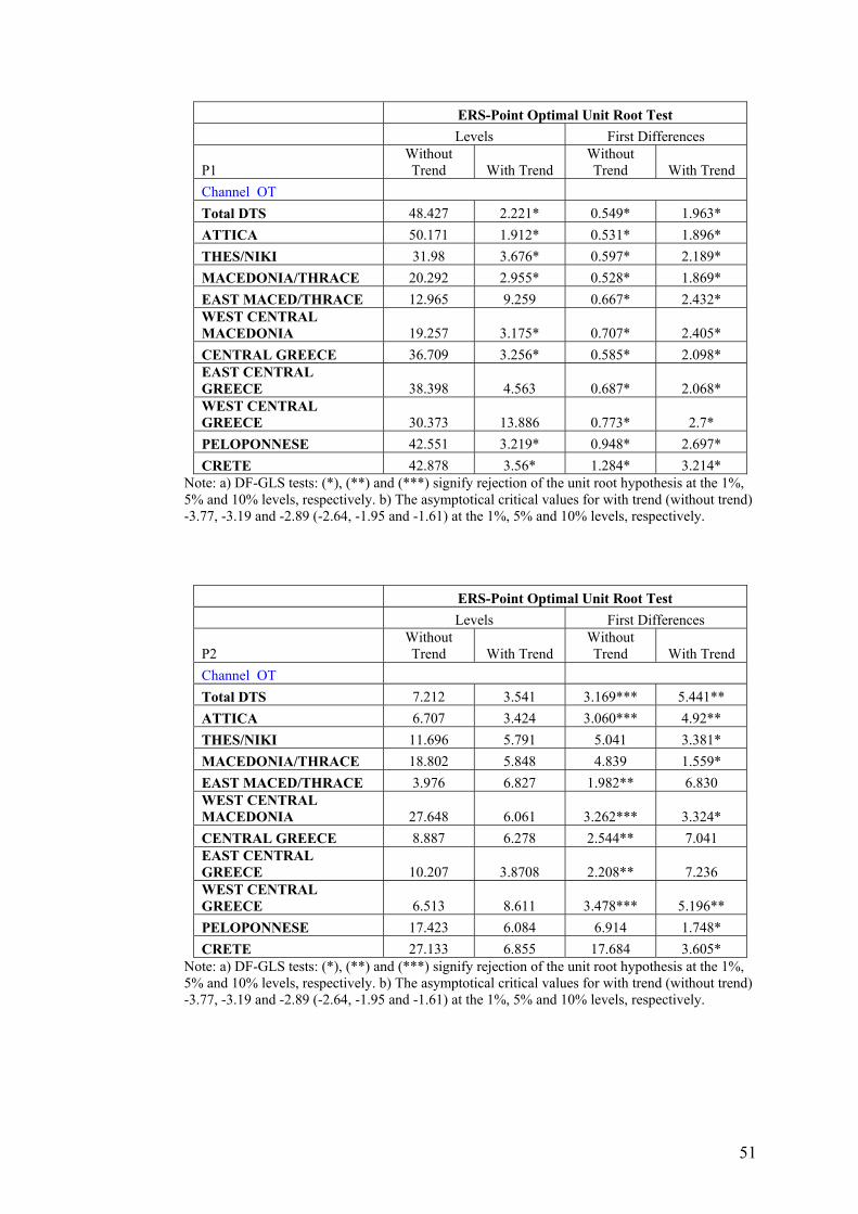
51
ERS-Point Optimal Unit Root Test Levels First Differences
P1 Without Trend With Trend
Without Trend With Trend
Channel OT Total DTS 48.427 2.221* 0.549* 1.963* ATTICA 50.171 1.912* 0.531* 1.896* THES/NIKI 31.98 3.676* 0.597* 2.189* MACEDONIA/THRACE 20.292 2.955* 0.528* 1.869* EAST MACED/THRACE 12.965 9.259 0.667* 2.432* WEST CENTRAL MACEDONIA 19.257 3.175* 0.707* 2.405* CENTRAL GREECE 36.709 3.256* 0.585* 2.098* EAST CENTRAL GREECE 38.398 4.563 0.687* 2.068* WEST CENTRAL GREECE 30.373 13.886 0.773* 2.7* PELOPONNESE 42.551 3.219* 0.948* 2.697* CRETE 42.878 3.56* 1.284* 3.214*
Note: a) DF-GLS tests: (*), (**) and (***) signify rejection of the unit root hypothesis at the 1%, 5% and 10% levels, respectively. b) The asymptotical critical values for with trend (without trend) -3.77, -3.19 and -2.89 (-2.64, -1.95 and -1.61) at the 1%, 5% and 10% levels, respectively.
Note: a) DF-GLS tests: (*), (**) and (***) signify rejection of the unit root hypothesis at the 1%, 5% and 10% levels, respectively. b) The asymptotical critical values for with trend (without trend) -3.77, -3.19 and -2.89 (-2.64, -1.95 and -1.61) at the 1%, 5% and 10% levels, respectively.
ERS-Point Optimal Unit Root Test Levels First Differences
P2 Without Trend With Trend
Without Trend With Trend
Channel OT Total DTS 7.212 3.541 3.169*** 5.441** ATTICA 6.707 3.424 3.060*** 4.92** THES/NIKI 11.696 5.791 5.041 3.381* MACEDONIA/THRACE 18.802 5.848 4.839 1.559* EAST MACED/THRACE 3.976 6.827 1.982** 6.830 WEST CENTRAL MACEDONIA 27.648 6.061 3.262*** 3.324* CENTRAL GREECE 8.887 6.278 2.544** 7.041 EAST CENTRAL GREECE 10.207 3.8708 2.208** 7.236 WEST CENTRAL GREECE 6.513 8.611 3.478*** 5.196** PELOPONNESE 17.423 6.084 6.914 1.748* CRETE 27.133 6.855 17.684 3.605*
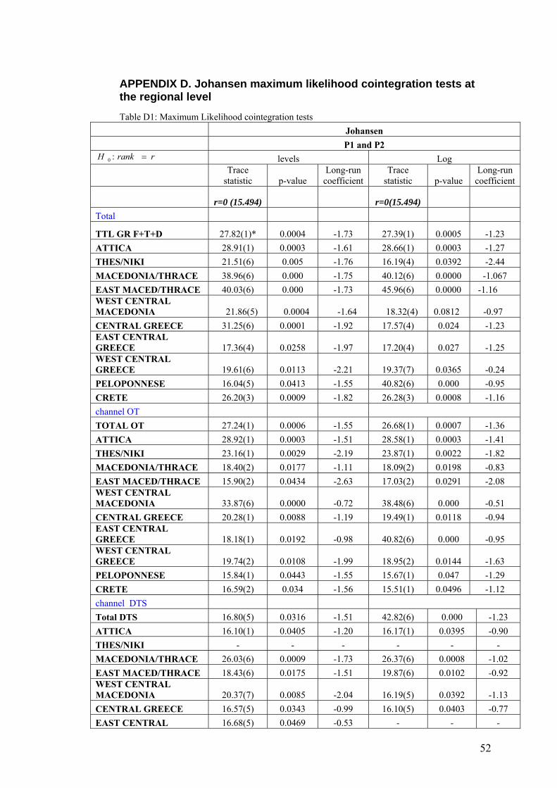
52
APPENDIX D. Johansen maximum likelihood cointegration tests at the regional level
Table D1: Maximum Likelihood cointegration tests Johansen P1 and P2
rrankH =:0 levels Log
Trace
statistic p-value Long-run
coefficient Trace
statistic p-value Long-run
coefficient
r=0 (15.494) r=0(15.494) Total
TTL GR F+T+D 27.82(1)* 0.0004 -1.73 27.39(1) 0.0005 -1.23 ATTICA 28.91(1) 0.0003 -1.61 28.66(1) 0.0003 -1.27 THES/NIKI 21.51(6) 0.005 -1.76 16.19(4) 0.0392 -2.44 MACEDONIA/THRACE 38.96(6) 0.000 -1.75 40.12(6) 0.0000 -1.067 EAST MACED/THRACE 40.03(6) 0.000 -1.73 45.96(6) 0.0000 -1.16 WEST CENTRAL MACEDONIA 21.86(5) 0.0004 -1.64 18.32(4) 0.0812 -0.97 CENTRAL GREECE 31.25(6) 0.0001 -1.92 17.57(4) 0.024 -1.23 EAST CENTRAL GREECE 17.36(4) 0.0258 -1.97 17.20(4) 0.027 -1.25 WEST CENTRAL GREECE 19.61(6) 0.0113 -2.21 19.37(7) 0.0365 -0.24 PELOPONNESE 16.04(5) 0.0413 -1.55 40.82(6) 0.000 -0.95 CRETE 26.20(3) 0.0009 -1.82 26.28(3) 0.0008 -1.16 channel ΟΤ TOTAL OΤ 27.24(1) 0.0006 -1.55 26.68(1) 0.0007 -1.36 ATTICA 28.92(1) 0.0003 -1.51 28.58(1) 0.0003 -1.41 THES/NIKI 23.16(1) 0.0029 -2.19 23.87(1) 0.0022 -1.82 MACEDONIA/THRACE 18.40(2) 0.0177 -1.11 18.09(2) 0.0198 -0.83 EAST MACED/THRACE 15.90(2) 0.0434 -2.63 17.03(2) 0.0291 -2.08 WEST CENTRAL MACEDONIA 33.87(6) 0.0000 -0.72 38.48(6) 0.000 -0.51 CENTRAL GREECE 20.28(1) 0.0088 -1.19 19.49(1) 0.0118 -0.94 EAST CENTRAL GREECE 18.18(1) 0.0192 -0.98 40.82(6) 0.000 -0.95 WEST CENTRAL GREECE 19.74(2) 0.0108 -1.99 18.95(2) 0.0144 -1.63 PELOPONNESE 15.84(1) 0.0443 -1.55 15.67(1) 0.047 -1.29 CRETE 16.59(2) 0.034 -1.56 15.51(1) 0.0496 -1.12 channel DTS Total DTS 16.80(5) 0.0316 -1.51 42.82(6) 0.000 -1.23 ATTICA 16.10(1) 0.0405 -1.20 16.17(1) 0.0395 -0.90 THES/NIKI - - - - - - MACEDONIA/THRACE 26.03(6) 0.0009 -1.73 26.37(6) 0.0008 -1.02 EAST MACED/THRACE 18.43(6) 0.0175 -1.51 19.87(6) 0.0102 -0.92 WEST CENTRAL MACEDONIA 20.37(7) 0.0085 -2.04 16.19(5) 0.0392 -1.13 CENTRAL GREECE 16.57(5) 0.0343 -0.99 16.10(5) 0.0403 -0.77 EAST CENTRAL 16.68(5) 0.0469 -0.53 - - -
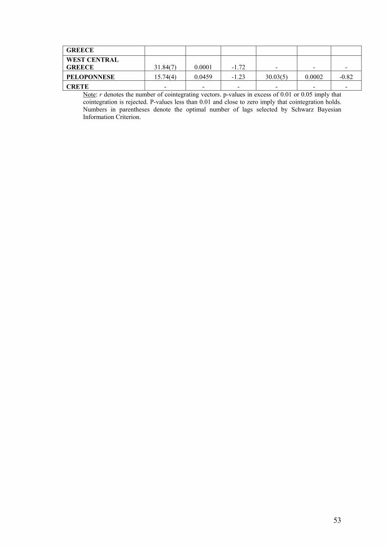
53
GREECE WEST CENTRAL GREECE 31.84(7) 0.0001 -1.72 - - - PELOPONNESE 15.74(4) 0.0459 -1.23 30.03(5) 0.0002 -0.82 CRETE - - - - - -
Note: r denotes the number of cointegrating vectors. p-values in excess of 0.01 or 0.05 imply that cointegration is rejected. P-values less than 0.01 and close to zero imply that cointegration holds. Numbers in parentheses denote the optimal number of lags selected by Schwarz Bayesian Information Criterion.