ATEX style emulateapj v. 10/09/06 - arXiv.org e-Print … Chatterjee, Ford, & Rasio Fig....

arX

iv:a

stro

-ph/

0703

166v

2 1

5 M

ay 2

008

Draft version May 15, 2008Preprint typeset using LATEX style emulateapj v. 10/09/06

DYNAMICAL OUTCOMES OF PLANET–PLANET SCATTERING

Sourav Chatterjee,1 Eric B. Ford,2,3,4 Soko Matsumura,1 and Frederic A. Rasio1

Draft version May 15, 2008

ABSTRACT

Observations in the past decade have revealed extrasolar planets with a wide range of orbital semi-major axes and eccentricities. Based on the present understanding of planet formation via core accre-tion and oligarchic growth, we expect that giant planets often form in closely packed configurations.While the protoplanets are embedded in a protoplanetary gas disk, dissipation can prevent eccen-tricity growth and suppress instabilities from becoming manifest. However, once the disk dissipates,eccentricities can grow rapidly, leading to close encounters between planets. Strong planet–planetgravitational scattering could produce both high eccentricities and, after tidal circularization, veryshort-period planets, as observed in the exoplanet population. We present new results for this sce-nario based on extensive dynamical integrations of systems containing three giant planets, both withand without residual gas disks. We assign the initial planetary masses and orbits in a realistic mannerfollowing the core accretion model of planet formation. We show that, with realistic initial conditions,planet–planet scattering can reproduce quite well the observed eccentricity distribution. Our resultsalso make testable predictions for the orbital inclinations of short-period giant planets formed viastrong planet scattering followed by tidal circularization.Subject headings: methods: n-body simulations, methods: numerical, (stars:) planetary systems,

(stars:) planetary systems: protoplanetary disks, planetary systems: formation —celestial mechanics

1. INTRODUCTION

The study of extrasolar planets and their propertieshas become a very exciting area of research over thepast decade. Since the detection of the planet 51 Peg b,more than 200 new planets (Butler et al. 2006, see alsohttp://exoplanet.eu/) have been detected and the largesky surveys planned for the near future can potentiallydetect many more. These detections have raised manyquestions about the formation and dynamical evolutionof planetary systems. The extrasolar planet populationcovers a much greater portion of the semimajor axis andeccentricity plane than was expected based on the plan-ets in our solar system (Lissauer 1995, Fig. 1). The pres-ence of many giant planets in highly eccentric orbits orin very short-period orbits (the “hot Jupiters”) is partic-ularly puzzling.

Different scenarios have been proposed to explain thehigh eccentricities. The presence of a distant compan-ion in a highly inclined orbit can increase the eccentric-ities of the planets around a star through Kozai oscilla-tions (Mazeh et al. 1997; Holman et al. 1997). However,this alone cannot explain the observed eccentricity dis-tribution (Takeda & Rasio 2005). Interaction with theprotoplanetary gas disk could either excite or damp theeccentricities depending on the properties of the diskand the orbits. However, the combined effects typi-cally result in eccentricity damping (Artymowicz 1992;Papaloizou & Terquem 2001; Goldreich & Sari 2003;Ogilvie & Lubow 2003). Migration of two planets and

1 Department of Physics and Astronomy, Northwestern Univer-sity, Evanston, IL 60208

2 Harvard-Smithsonian Center for Astrophysics, Mail Stop 51,60 Garden Street, Cambridge, MA 02138

3 Department of Astronomy, University of Florida, 211 BryantSpace Science Center, P.O. Box 112055, Gainesville, FL, 32611

4 Hubble Fellow

trapping in a mean-motion resonance (MMR) can alsopump up the eccentricities efficiently, but this mech-anism requires strong damping at the end or termi-nation of migration right after trapping in resonance(Lee & Peale 2002) or else it leads to planet scattering(Sandor & Kley 2006). Zakamska & Tremaine (2004)proposed inward propagation of eccentricity after theouter planets are excited to high eccentricities following aclose encounter with a passing star. Using typical valuesfor such interactions with field stars in the solar neighbor-hood, however, they do not get very high eccentricities.Papaloizou & Terquem (2001); Terquem & Papaloizou(2002); Black (1997) propose a very different formationscenario for planets from protostellar collapse in whichboth hot Jupiters and eccentric planets at higher semi-major axes are formed naturally; this scenario, however,cannot form sub-Jupiter-mass planets.

In this paper, we explore another promising wayto create high eccentricities: strong gravitational scat-tering between planets in a multi-planet system un-dergoing dynamical instability (Rasio & Ford 1996;Weidenschilling & Marzari 1996; Lin & Ida 1997). Ac-cording to the model of oligarchic growth, planetesi-mals form in a nearly maximally packed configurationin the protoplanetary disk, followed by gas accretion(Goldreich et al. 2004; Ida & Lin 2004b; Kokubo & Ida2002). Once the disk dissipates, mutual planetary per-turbations (“viscous stirring”) of the planetesimals willlead to eccentricity growth, orbit crossing, and even-tually close encounters between the big bodies in thedisk (Ford & Chiang 2007; Levison & Morbidelli 2007).While planetary systems with more than two planetscan not be provably stable, they can remain stable forvery long timescales depending on their initial separa-tions (Chambers et al. 1996; Marzari & Weidenschilling2002). A sufficiently massive disk can prevent interacting

http://arXiv.org/abs/astro-ph/0703166v2

http://exoplanet.eu/

2 Chatterjee, Ford, & Rasio

Fig. 1.— Semi-major axis vs eccentricity for the detected planets.The sizes of the points are proportional to the minimum masses(m sin i) of the corresponding planets. The size of a Jupiter massplanet is shown at the left top corner for reference. The starsrepresent the four giant planets in our solar system (for these thesizes do not indicate their mass). The open circles show the planetsdetected by radial velocity surveys. The triangles show planetsdetected by micro-lensing or direct imaging. Planets with poorlyconstrained eccentricities are plotted above e = 1. A horizontalline is drawn at e = 1 to guide the eye. Note the logarithmic scalefor the semi-major axis.

planets from acquiring large eccentricities and developingcrossing orbits. However, once the gas disk is sufficientlydissipated, and the planetesimal disk depleted, the eccen-tricities of the planets can grow to high values, possiblyleading to strong planet–planet scattering and a phaseof chaotic evolution that dramatically alters the orbitalstructure of the system (Lin & Ida 1997; Ford & Chiang2007; Levison & Morbidelli 2007).

The detection of close-in planets with orbital periodsas short as ∼ 1 d, the so-called “hot Jupiters” (and,more recently, hot Neptunes and super-Earths), was an-other major surprise. Giant planets are most likely toform at much larger separations, beyond the ice line ofthe star where there can be enhanced dust production(Kokubo & Ida 2002; Ida & Lin 2004b). It is widely be-lieved that the giant planets form beyond the ice line andthen migrate inwards to form the hot Jupiters we observetoday. Different stopping mechanisms of inward migra-tion have been proposed to explain the hot Jupiters,but it is unclear why they pile up at just a few solarradii around the star, rather than continue migrating andeventually accrete onto the star.

Strong gravitational scattering between planets in amulti-planet system may provide another way to cre-ate these close-in planets (Rasio & Ford 1996). A fewof the planets scattered into very highly eccentric orbitscould have sufficiently small periastron distances thattidal circularization takes place, giving rise to the hotJupiters. The currently observed edge in the mass-perioddiagram is very nearly at the ideal circularization radius(twice the Roche limit), providing support for this model(Ford & Rasio 2006). Faber et al. (2005) finds that theseviolent passages might not destroy the planets, even ifmass loss occurs.

Previous studies have investigated gas free sys-tems with two planets around a central star ex-tensively (Rasio & Ford 1996; Ford et al. 2001, 2003;Ford & Rasio 2007) and have also begun to investigatethe dynamics of two planets in the presence of a gas diskby using simplified prescriptions for dissipative effects(Moorhead & Adams 2005). The observed eccentricitydistribution is not easily reproduced by two equal-massplanets (Ford et al. 2001). However, strong scatteringof two unequal-mass planets could explain the observedeccentricities of most observed exoplanets (Ford et al.2003; Ford & Rasio 2007).

A system with three planets is qualitatively differentthan one with two planets. In two-planet systems, thereis a sharp boundary between initial conditions that areprovably Hill stable and initial conditions that quicklylead to a close encounter (Gladman 1993). Moreover,for two Jupiter-mass planets in close to circular orbits,this boundary lies where the ratio of orbital periods isless than 2:1. If these planets formed further apart, thena slow and smooth migration could lead to systems be-coming trapped in a 2:1 MMR before triggering an insta-bility (Lee & Peale 2002; but see Sandor & Kley 2006).These stability properties are in sharp contrast to thoseof systems with three or more planets, for which thereis no sharp stability boundary. These systems can be-come unstable even for much wider initial spacings andthe timescale to the first close encounter can be verylong (Chambers et al. 1996). Even if all pairs of adja-cent planets in the system are stable according to thetwo-planet criterion, the combined system can evolve ina chaotic (but apparently bounded) manner for an arbi-trarily long time period before instability sets in. Thistimescale to instability can easily exceed other timescalesof interest here such as those for the formation of giantplanets, orbital migration, or dispersal of the gas disk.Therefore, the stability properties of three-planet sys-tems can be studied with long-term orbital integrationswithout the need to implement any additional physics.

A pioneering study of the stability and final or-bital properties of three-planet systems was performedby Marzari & Weidenschilling (2002, hereafter MW02).They explored the basic nature of instabilities arising insystems with three giant planets around a central solar-like star, and they determined the final orbital propertiesafter one planet is ejected. This study used highly ide-alized initial conditions with three equal-mass planets orwith one arbitrary mass distribution (middle planet twiceas massive as the other two). It was also computationallylimited to a rather small ensemble of systems.

Our two main goals in this new work were to extendthe work of MW02 by using more realistic initial con-ditions (see §2) and to perform a much more extensivenumerical survey in order to fully characterize the sta-tistical properties of outcomes for unstable three-planetsystems. Given the chaotic nature of the dynamics, oneneeds to integrate many independent systems to char-acterize the statistical properties of the final planetaryorbits (see a detailed analysis for the dependence of var-ious statistics on the sample size in Appendix A; seealso Adams & Laughlin 2003). Each system has to beintegrated for a long time, so that it reaches the orbit-crossing unstable phase and later evolves into a new, sta-ble configuration. Given the rapid increase in computing

Dynamical Outcomes of Planet–Planet Scattering 3

power, we are now able to perform significantly moreand longer integrations to obtain much better statisticalresults than was possible just a few years ago.

In addition, we also present the results of new simu-lations for systems of three giant planets still embeddedin a residual gas disk. Here our goal is different: wefocus on the transition from gas-dominated to gas-freesystems, in the hope of better justifying the (gas-free)initial conditions adopted in the first part of our work.However, implementing the physics of planet-disk inter-actions implies a considerably higher computational cost,preventing us from doing a complete statistical study ofoutcomes at this point.

2. GAS-FREE SYSTEMS WITH THREE GIANT PLANETS

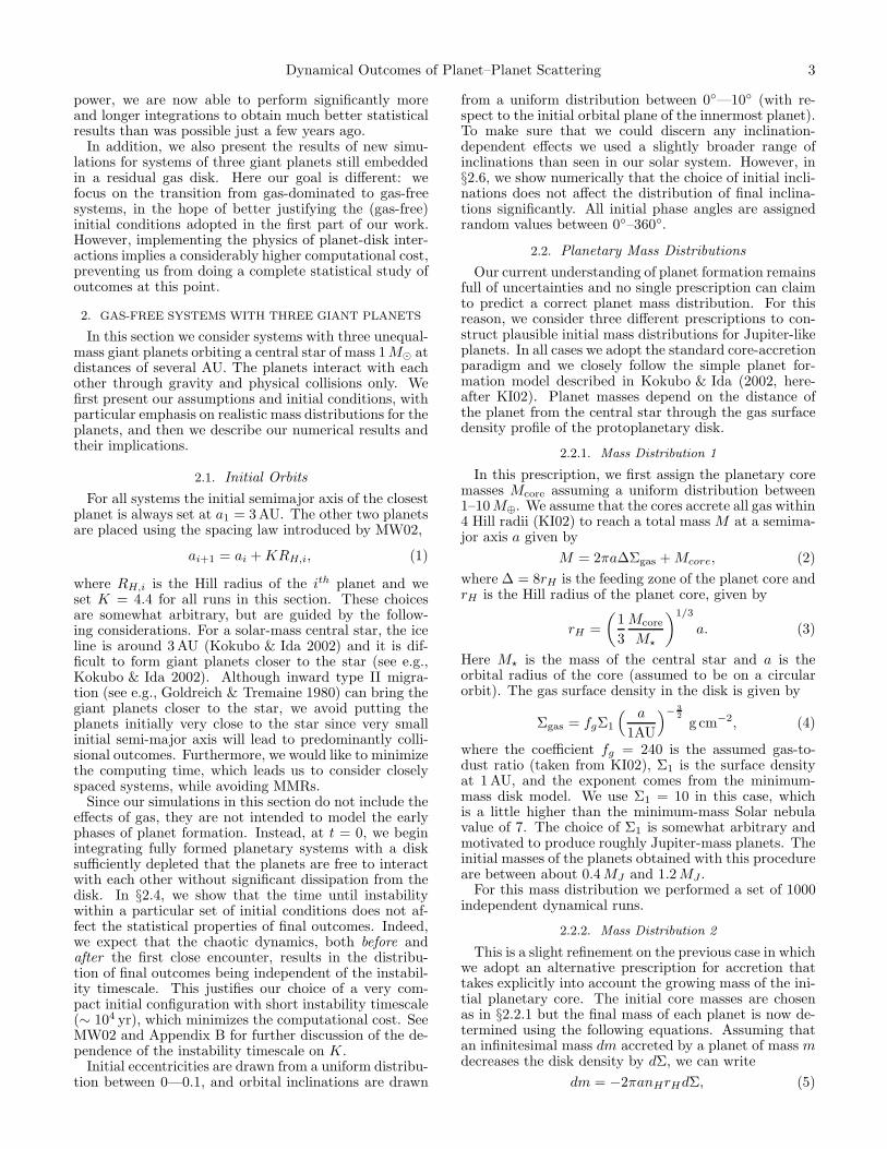
In this section we consider systems with three unequal-mass giant planets orbiting a central star of mass 1 M⊙ atdistances of several AU. The planets interact with eachother through gravity and physical collisions only. Wefirst present our assumptions and initial conditions, withparticular emphasis on realistic mass distributions for theplanets, and then we describe our numerical results andtheir implications.

2.1. Initial Orbits

For all systems the initial semimajor axis of the closestplanet is always set at a1 = 3 AU. The other two planetsare placed using the spacing law introduced by MW02,

ai+1 = ai + KRH,i, (1)

where RH,i is the Hill radius of the ith planet and weset K = 4.4 for all runs in this section. These choicesare somewhat arbitrary, but are guided by the follow-ing considerations. For a solar-mass central star, the iceline is around 3 AU (Kokubo & Ida 2002) and it is dif-ficult to form giant planets closer to the star (see e.g.,Kokubo & Ida 2002). Although inward type II migra-tion (see e.g., Goldreich & Tremaine 1980) can bring thegiant planets closer to the star, we avoid putting theplanets initially very close to the star since very smallinitial semi-major axis will lead to predominantly colli-sional outcomes. Furthermore, we would like to minimizethe computing time, which leads us to consider closelyspaced systems, while avoiding MMRs.

Since our simulations in this section do not include theeffects of gas, they are not intended to model the earlyphases of planet formation. Instead, at t = 0, we beginintegrating fully formed planetary systems with a disksufficiently depleted that the planets are free to interactwith each other without significant dissipation from thedisk. In §2.4, we show that the time until instabilitywithin a particular set of initial conditions does not af-fect the statistical properties of final outcomes. Indeed,we expect that the chaotic dynamics, both before andafter the first close encounter, results in the distribu-tion of final outcomes being independent of the instabil-ity timescale. This justifies our choice of a very com-pact initial configuration with short instability timescale(∼ 104 yr), which minimizes the computational cost. SeeMW02 and Appendix B for further discussion of the de-pendence of the instability timescale on K.

Initial eccentricities are drawn from a uniform distribu-tion between 0—0.1, and orbital inclinations are drawn

from a uniform distribution between 0◦—10◦ (with re-spect to the initial orbital plane of the innermost planet).To make sure that we could discern any inclination-dependent effects we used a slightly broader range ofinclinations than seen in our solar system. However, in§2.6, we show numerically that the choice of initial incli-nations does not affect the distribution of final inclina-tions significantly. All initial phase angles are assignedrandom values between 0◦–360◦.

2.2. Planetary Mass Distributions

Our current understanding of planet formation remainsfull of uncertainties and no single prescription can claimto predict a correct planet mass distribution. For thisreason, we consider three different prescriptions to con-struct plausible initial mass distributions for Jupiter-likeplanets. In all cases we adopt the standard core-accretionparadigm and we closely follow the simple planet for-mation model described in Kokubo & Ida (2002, here-after KI02). Planet masses depend on the distance ofthe planet from the central star through the gas surfacedensity profile of the protoplanetary disk.

2.2.1. Mass Distribution 1

In this prescription, we first assign the planetary coremasses Mcore assuming a uniform distribution between1–10 M⊕. We assume that the cores accrete all gas within4 Hill radii (KI02) to reach a total mass M at a semima-jor axis a given by

M = 2πa∆Σgas + Mcore, (2)

where ∆ = 8rH is the feeding zone of the planet core andrH is the Hill radius of the planet core, given by

rH =

(

1

3

Mcore

M⋆

)1/3

a. (3)

Here M⋆ is the mass of the central star and a is theorbital radius of the core (assumed to be on a circularorbit). The gas surface density in the disk is given by

Σgas = fgΣ1

( a

1AU

)−3

2

g cm−2, (4)

where the coefficient fg = 240 is the assumed gas-to-dust ratio (taken from KI02), Σ1 is the surface densityat 1 AU, and the exponent comes from the minimum-mass disk model. We use Σ1 = 10 in this case, whichis a little higher than the minimum-mass Solar nebulavalue of 7. The choice of Σ1 is somewhat arbitrary andmotivated to produce roughly Jupiter-mass planets. Theinitial masses of the planets obtained with this procedureare between about 0.4 MJ and 1.2 MJ .

For this mass distribution we performed a set of 1000independent dynamical runs.


This is a slight refinement on the previous case in whichwe adopt an alternative prescription for accretion thattakes explicitly into account the growing mass of the ini-tial planetary core. The initial core masses are chosenas in §2.2.1 but the final mass of each planet is now de-termined using the following equations. Assuming thatan infinitesimal mass dm accreted by a planet of mass mdecreases the disk density by dΣ, we can write

dm = −2πanHrHdΣ, (5)


where nH is the number of Hill radii over which the massis accreted. The final mass M of a planet at a distancea from the star, starting with a core mass Mcore can beobtained by integrating Eq. 5 as follows,

∫ M

Mcore

m−1/3dm = −2πnHa2 1

3M1/3⋆

∫ 0

Σi

dΣ, (6)

where Σi is the initial disk surface mass density. SolvingEq. 6 and replacing Σi from Eq. 4 we find

M =

(

4πnHa2

M1/3⋆ 34/3

fgΣ1

( a

1AU

)−3/2

+ m2/3c

)3/2

. (7)

Here we use nH = 8, i.e., we assume that the core ac-cretes all mass within 4 Hill radii on either side. We usethe same values for fg and Σ1 from §2.2.1.

For this mass distribution we have integrated a smallerset of 224 systems.


We expect that the final distributions of different or-bital properties may vary significantly with different ini-tial mass distribution. To further test this mass depen-dence, we created a third set of systems with a broaderplanet mass distribution. Here we assign planetarymasses exactly as in §2.2.1, but the initial core masses arechosen differently. We sample Mcore from a distribution

of masses between 1–100 M⊕ uniform in M1/5core, while as-

suming again that these cores accrete all gas within 8Hill radii. The exponent in the core mass distributionand the surface density at 1 AU, Σ1 = 15, are chosensomewhat arbitrarily with the goal to obtain an initialmass distribution that peaks around a Jupiter mass butwith a tail extending up to several Jupiter masses. Thechoices above produce initial masses spanning about anorder of magnitude, in the range 0.4 MJ–4 MJ . More-over, the distribution for higher-mass planets resemblesthe mass distribution of observed exoplanets (see §2.8).

For this mass distribution we have integrated a set of500 systems.

2.3. Numerical Integrations

We integrate each system for 107 yr, which is 2 × 106

times the initial period of the closest planet (T1,i), andtypically much longer than the timescale for the onset ofinstability. We use the hybrid integrator of MERCURY6.2(Chambers 1999) and integrate the orbits symplecticallywhile there is no close encounter, with a time-step of 10days, but switching to a Bulirsch-Stoer (BS) integrationas soon as two planets have a close approach (defined tobe closer than 3 Hill radii). Runs with poor energy con-servation (|∆E/E| ≥ 0.001) with the hybrid integratorare repeated using the BS integrator throughout with thesame |∆E/E| tolerance. This happens in ∼ 30% of allruns, but our conclusions are not affected even if we re-ject these systems. We find that, in all systems, at leastone planet is eventually ejected. Note that, for three-planet systems, following an ejection the remaining twoplanets may or may not be dynamically unstable. There-fore, we do not stop the integration following an ejection.Instead, we continue all integrations for two planets un-til a fixed stopping time of 107 yr. For systems with tworemaining planets we check for Hill stability using the

Fig. 2.— Time evolution of semi-major axes and eccentricities fortwo randomly chosen typical simulations. The solid (black), dotted(red), and dashed (green) lines show the orbital elements for theinitially closest (a1, e1), middle (a2, e2), and furthest (a3, e3)planets. The top pair of panels show a realization where the firstplanet is ejected at ∼ 4.1× 104 T1,i, and the integration concludeswith two planets in provably stable orbits. The semi-major axesfor both P2 and P3 remain constant and the eccentricities oscillatestably on a secular timescale. The bottom pair shows anotherrealization where P3 collides with P1 at ∼ 4.2 × 103 T1,i; e2 keeps

increasing until, a little before 105 T1,i P2 gets ejected, leaving asingle planet in the system. Since a single orbit is always stablewe stop the integration following this ejection. Numbers in thesubscript represent the positional sequence of the planets startingfrom the star and letters “i” and “f” mean initial and final values,respectively, in all plots.

known semi-analytic criterion (Gladman 1993). In oursimulations about 9% of systems were not provably Hillstable at the integration stopping time. We discard thosefrom our analysis. When a single planet remains (follow-ing a second ejection or when a collision took place), theintegration is of course stopped immediately.

For systems with two remaining dynamically stableplanets the orbits can still evolve on a secular timescale(typically ∼ 105–106 yr for our simulated systems)much larger than the dynamical instability timescale(Adams & Laughlin 2006a; see also Murray & Dermott2000, Ch 7). We study these systems with two remain-ing stable planets by integrating the secular perturba-tion equations for a further 109 yr with the analyticalformalism developed in Ford et al. (2000). Note that themore standard formulation for Solar system dynamics(Murray & Dermott 2000) is not appropriate for theseplanetary systems because a significant fraction presentvery high eccentricities and inclinations. We find thatfor most of our simulated systems our chosen integra-tion stopping time effectively sampled the full parameterspace (see detailed discussion in §2.9).

We treat collisions between planets in the followingsimple way (“sticky-sphere” approximation). A collisionis assumed to happen when the distance between twoplanets becomes less than the sum of their physical radii.We assume Jupiter’s density (1.33 g cm−3) for all plan-ets when determining the radius from the mass. Aftera collision the two planets are replaced by a single oneconserving mass and linear momentum. Because we ac-


Fig. 3.— Cumulative distributions showing initial and final ec-centricities of the planets. Top and bottom panels show the initialand final cumulative eccentricity distributions, respectively. In thetop panel solid (black), dotted (red) and dashed (blue) lines rep-resent the closest, middle, and furthest planets, respectively. Theyare on top of each other because the initial eccentricity distributionis the same for all of the planets. In the bottom panel solid (black)and dotted (red) lines represent the final inner and outer planets,respectively. The dashed (blue) line shows all remaining planets infinal stable orbits.

count for collisions, our results are not strictly scale free.However, we find that collisions are relatively rare for ourchoice of initial conditions, so we still present all resultswith lengths scaled to a1,i and times scaled to T1,i.

Since Mass Distribution 1 corresponds to our largestset of runs, we first show our results from this set indetail in the following subsections (§2.4 – §2.7). Resultsfor the other two sets are summarized in §2.8.

2.4. Overview of Results

In Fig. 2 we show a couple of randomly selected, rep-resentative examples of the dynamical evolution of thesesystems, showing both chaotic phases and stable finalconfigurations. Note the order-of-magnitude differencein timescale to first orbit crossing, illustrating the broadrange of instability timescales (see also the discussionin Appendix B). We find that strong scattering be-tween planets increases the eccentricities very efficiently(Fig. 3). The median of the eccentricity distribution forthe final inner planets is 0.4. The median eccentricityfor the final outer planets is 0.37, that for all simulatedplanets in their final stable orbits, is ∼ 0.38.

We compare our results with the observed eccentricitydistribution of detected exoplanets in Fig. 4. For a moremeaningful comparison we restrict our attention to ob-served planets with masses greater than 0.4 MJ , similarto the lower mass cut-off in our simulated systems. Wealso place an upper limit on the semimajor axis at 10 AUfor the simulated final planet population to address theobservational selection effects against discovering plan-ets with large orbital periods. Similarly, since planetsclose to the central star can be affected by additionalphysics beyond the scope of this study (e.g., tides, gen-eral relativistic effects; see Adams & Laughlin 2006b) wealso omit observed close-in planets with semimajor axes

Fig. 4.— Comparison between the simulated and observed ex-oplanet populations. The solid (black) line shows the cumulativedistribution of the eccentricities of the remaining planets in theirfinal stable orbits. The dashed (red) line is that for the observedpopulation. For this comparison we employ a lower mass cut-off of0.4 MJ on the observed population addressing the fact that we donot have lower mass planets in our simulations. We also consideronly the simulated planets that are finally within 10 AU from thestar to address the fact that in the observed population we do nothave planets further out. We also employ a lower semi-major axiscut-off of 0.1 a1,i on the observed population.

Fig. 5.— Cumulative frequency plots of semi-major axes of theinitial (top panel) and final (bottom panel) planets. Vertical solid(black), dotted (red) and dashed (blue) lines show the initial val-ues in the top panel. These are vertical lines because the initialsemi-major axes of the closest, middle and outer planets do nothave a spread. Solid (black) and dotted (red) curves in the bot-tom panel show the final inner and outer planets’ semi-major axes,respectively.

below 0.1 a1,i.As seen in Fig. 3 and Fig. 4, our simulations slightly

overestimate the eccentricities of the planetary orbits.However, the slopes of the cumulative eccentricity dis-tributions at higher eccentricity values are similar. In arealistic planetary system, there might be damping ef-


Fig. 6.— Final semi-major axis versus eccentricity plot. Alllengths are scaled by the initial closest planet semi-major axis (herea1,i = 3.0AU). Black solid circles and red open stars representthe final inner and outer planets, respectively. Solid lines showdifferent constant periapse lines with values 0.1 and 0.5. Note thehigh eccentricities and the close approaches towards the centralstar. The empty wedge shaped region in the a-e plane at higheccentricities is due to the requirement for orbital stability.

TABLE 1Comparison of Eccentricity

Distributions

D P

Mass distribution 1 0.113 0.15Mass distribution 2 0.171 0.01Mass distribution 3 0.087 0.32

a For each mass distribution, wecompare the final eccentricity dis-tribution of the simulated popula-tion with the observed exoplanetpopulation (Figs. 4, 18). Usingthe kstwo function in Numerical

Recipes, we calculate the two-sample Kolmogorv-Smirnov statis-tic, D, and the corresponding prob-ability, P . In each case, the highvalue of P indicates that we can notreject the null hypothesis that bothsamples were drawn from the samepopulation.

fects from lingering gas, dust or planetesimals in a pro-toplanetary disk. While our simplified models alreadycome close to matching the eccentricity distribution ofobserved planets, including damping may further im-prove this agreement. To be more quantitative, we per-form a Kolmogorov-Smirnov (KS) test and find that wecannot rule out the null hypothesis (that the two pop-ulations are drawn from the same distribution) at the85% level (Table 1). In §2.8, we will show that a broaderinitial distribution of planet masses results in an evenbetter match to the observed eccentricity distribution.

The top and bottom panels in Fig. 5 show the cumu-lative distributions of the initial vs final semi-major axesfor the planets. The planet that is closest to the star ini-tially may not remain closest at the end of the dynam-

Fig. 7.— Left panel: cumulative frequency plots for the finaleccentricities of the two subgroups, Group 1 (solid line) and Group2 (dashed line). Right panel: cumulative frequency plots for thefinal semi-major axes of the two subgroups, Group 1 (solid line)and Group 2 (dashed line). KS statistics results, D and P are alsoquoted for each of the above. D and P are as defined in Table 1.

ical evolution. In fact, all three planets, independentof their initial positions, have roughly equal probabil-ity of becoming the innermost planet in the final stableconfiguration when the planet masses are not very dif-ferent. In 20% of the final stable systems, we find asingle planet around the central star, two planets havingbeen lost from the system either through some combi-nation of collisions and dynamical ejection. The othersystems have two giant planets remaining in stable or-bits. We find that the planets in the outer orbits show atendency for higher eccentricities correlating with largersemi-major axes (Fig. 6). We now know that many ofthe current observed exoplanets may have other planetsin distant orbits (Wright et al. 2007). From our resultswe expect that planets scattered into very distant boundorbits will have higher eccentricities. Long-term radialvelocity monitoring should be able to test this predic-tion.

Next, we investigate to what extent the final orbitalproperties depend on the instability timescale (equiv-alently, on how closely packed the initial configurationwas). For each system we integrated in §2.2.1, we notedthe first time when the semi-major axis of any one ofthe planets in the system changed by at least 10%. Weuse this as a measure of the dynamical instability growthtimescale. Then, we divide the set into two subgroups,based on whether this growth time was below (Group 1)or above (Group 2) its median value (so 50% of the in-tegrated systems are in each group). Fig. 7 comparesthe final eccentricity and semi-major axis distributionsbetween the two groups. We find that the distributionsare indistinguishable, demonstrating that the final (ob-servable) orbital properties are not sensitive to when ex-actly a particular system became dynamically unstable,as long as the dynamics was sufficiently active (ensur-ing that close encouters occur) and avoiding initial con-ditions so closely packed that physical collisions wouldbecome dominant. This result is hardly surprising since


Fig. 8.— Cumulative histogram of the pericenter distance ofthe initial (top panel) and final (bottom panel) planets bound tothe star. In the top panel the solid, dotted and dashed lines showthe pericenter distributions of the initial closest, middle and thefurthest planets, respectively. In the bottom panel the solid anddotted lines show the same for the final stable inner and the outerplanets with their semi-major axes less than 10AU. The dashedmagenta line shows the pericenter distribution of the observed ex-oplanet population for comparison purposes.

we expect the chaotic evolution to efficiently erase anymemory of the initial orbital parameters. Our resultscan therefore be taken as representative of the dynam-ical outcome for analogous systems with an even largerinitial spacing between planets (but avoiding mean mo-tion resonances; see Appendix B). In practice, perform-ing a large number of numerical integrations for thesemore widely spaced initial configurations would be pro-hibitively expensive (see Appendix B).

2.5. Hot Jupiters from Planet–Planet Scattering

We find that a significant fraction of systems emergewith planets in orbits having very small periastron dis-tances. Fig. 6 shows the final positions of the planetsthat are still bound to the central star in the a−e plane.The solid lines represent different constant pericenter dis-tances. Note that the planets show weak correlationsbetween the eccentricity and the semi-major axis. Forthe inner planets, a lower semi-major axis tends to im-ply higher eccentricity, while the outer planets show anopposite trend. The final inner and outer planets formtwo clearly separated clusters of points in the a−e planedue to stability considerations.

Fig. 8 shows the cumulative distribution of the pe-riastron distances of the final bound planets aroundthe star. For the sake of comparison, we also showthe pericenter distribution of all observed exoplanetsin Fig. 8. We see that 10% of the systems harborplanets with periapse distances ≤ 0.05a1,i, whereas,a few (∼ 2%) harbor planets with periapse distances≤ 0.01a1,i. Since we do not include tidal effects, we can-not compare this quantitatively with the observed pop-ulation. However, this is consistent with the ∼ 5% ofobserved planets with semi-major axes within 0.03 AU.If the initial semi-major axes are sufficiently small tidal

Fig. 9.— Cumulative distribution showing initial and final or-bital inclinations of the planets with respect to the initial invari-able plane. In the top panel the solid (black) and the dotted (red)lines represent the initial and final RMS inclination distributions ofthe planet orbits with respect to the initial invariable plane. In themiddle panel solid (black), dotted (red) and dashed (blue) lines rep-resent the closest, middle and furthest planets, respectively. Thebottom panel shows the final orbital inclination distributions of theremaining planets in the system. The solid (black), and the dot-ted (red) lines represent the inner and outer planets, respectively.The dashed (blue) line represents the relative angles between thetwo remaining planetary orbits. Note that the final closer planets,which are the planets more easily observable in a planetary sys-tem, statistically have higher inclinations. Note, that the relativeinclinations between the planetary orbits are also quite high.

forces could then become important and a planet ona highly eccentric orbit could be circularized to pro-duce a hot Jupiter (Ford & Rasio 2006; Faber et al. 2005;Rasio & Ford 1996; Weidenschilling & Marzari 1996;Marzari & Weidenschilling 2002). However, recall thatsystems with much smaller values of a1,i would also leadto more physical collisions than in our simulations. More-over, a full numerical study of this scenario should in-clude tidal dissipation as part of the dynamical integra-tions, and possibly also include additional physics suchas GR effects, etc. (Nagasawa et al. 2008).

2.6. Planets on High-inclination Orbits

Since the star and planets get their angular momentafrom the same source, planetary orbits are generally ex-pected to form in a coplanar disk perpendicular to thestellar spin axis. In Fig. 9, we compare the distributionsof the final inclination angles. Here each angle reportedis the absolute value of the orbital inclination measuredwith respect to the initial invariable plane, defined asthe plane perpendicular to the initial total angular mo-mentum vector of the planetary orbits. Note that thedirection of the initial total angular momentum can dif-fer from the direction of the total angular momentum ofthe bound planets at the end of a simulation, since plan-ets are frequently ejected from the system, carrying awayangular momentum.

Strong scattering between planets often increases incli-nations of the orbits, leading to a higher final RMS valueof planet inclinations compared to the initial configura-tion (Fig. 9, top panel). In general, the inclinations tend


Fig. 10.— Initial RMS inclination vs final inclination of the inner-most planet. Note that the final closer planet orbital inclination islargely insensitive to the initial RMS inclination.

to increase for all planets. The middle and bottom pan-els in Fig. 9 show the initial and final inclinations of theorbits of individual planets, respectively. The inclinationof the final inner planet is typically larger than that ofthe final outer planet (Fig. 9, bottom panel).

Our results show that strong planet–planet scatteringcan dramatically affect the coplanarity of some plane-tary systems (Fig. 9, bottom panel). Since the timescalefor tidal damping of inclinations is usually much greaterthan the age of the stars (Winn et al. 2005), significantlyincreased inclinations could be found in some plane-tary systems that have gone through strong gravitationalscattering phases in their lifetimes. Measuring a poor de-gree of alignment among the planetary orbits in multiple-planet systems, or between the angular momentum of oneplanet and the spin axis of its host star, could be usedto identify systems that have undergone a particularlytumultuous dynamical history.

If a system were initially assigned to a strictly copla-nar configuration, then angular momentum conservationdictates that it would remain coplanar always. How-ever, away from this trivial limit, we expect little corre-lation between the initial and final inclinations, given thechaotic nature of the dynamics. We test this hypothesishere by investigating the correlation between the initialand final inclinations of all planets in our simulations.We find that the final inclination of the inner planetindeed does not depend on the initial RMS inclination(Fig. 10). We can quantify the amount of correlationbetween the initial RMS inclination and the final orbitalinclination of the final inner planet using the bivariatecorrelation coefficient. The bivariate correlation coeffi-cient (rxy) for two variables x and y, is given by thefollowing equation,

rxy =Cov(x, y)

sd(x)sd(y), (8)

where Cov(x, y) is the covariance of x and y, and sd(x) orsd(y) is the standard deviation of x or y. We find that thecorrelation coefficient between the initial RMS and the

Fig. 11.— Pericenter distance vs inclination of the final innerplanets. The open dots show the final positions of the final innerplanet in the pericenter-inclination plane. The filled disks (blue)and triangles (red) represent the mean orbital inclination of the in-ner planet and the final RMS inclinations, respectively. The meansare obtained for bins of equal population (nbin = 50). We observea weak anti-correlation between the pericenter and the inclination.

final inner planet orbital inclinations is riRMS,iclose =0.05. The low value of r confirms that the high finalinclinations are not merely a reflection of the initial con-ditions. As long as the planetary system is not strictlycoplanar initially, strong planet–planet scattering can in-crease the orbital inclinations of some systems signifi-cantly.

The final inclination of the inner planet, which is themost easily observable, shows a weak anti-correlationwith the pericenter distance of its orbit (Fig. 11): lowerpericenter orbits tend to have higher inclinations. Thecorrelation coefficient in this case is rrp,iclose = −0.13(Eq. 8).

For our solar system, the angle between the spin axisof the Sun and the invariable plane is ≃ 6◦. The an-gle between the stellar rotation axis and the orbitalangular momentum of a transiting planet (λ) can beconstrained via the Rossiter-McLaughlin effect. Obser-vations have measured λ sin i for five systems (Winn2006b): −4.4◦±1.4◦ for HD 209458b (Winn et al. 2005),−1.4◦±1.1◦ for HD 189733b (Winn et al. 2006), 11◦±15◦

for HD 149026b (Wolf et al. 2007), 30◦±21◦ for TrES-1b(Narita et al. 2007a), and, most recently, 62◦ ± 25◦ forHD 17156b (Narita et al. 2007b). Our study implies thatplanetary systems with a tumultuous dynamical historywill sometimes show a large λ. Therefore, we look for-ward to precise measurements of λ for many planetarysystems to determine the fraction of planets among theexoplanet population with a significant inclination. Inparticular HD 17156b is very interesting in this regard,since the potentially high λ together with the high ec-centricity (e = 0.67) strongly indicates a dynamical scat-tering origin for this planet. Measurements of λ wouldbe particularly interesting for the massive short-periodplanets (m > MJ), the very-short period giant plan-ets (P < 2.5 d), or the eccentric short period planets,since these planets might have a different formation his-


tory than the more common short-period planets withm ≃ 0.5MJ in nearly circular orbits.

2.7. Mean Motion Resonances

The radial-velocity planet population currently in-cludes 20 multi-planet systems and at least 5 of those sys-tems are in MMR (4 appear to be in a 2:1 MMR). MMRscan have strong effects on the dynamical evolution andstability of planetary systems. The 2:1 MMR is particu-larly interesting given the proximity of the two orbits andthe increased possibility for close encounters that couldresult in strong gravitational scattering between the twoplanets (Sandor & Kley 2006; Sandor et al. 2007).

It is widely believed that MMRs between two or moreplanets in a planetary system arise naturally from mi-gration. Convergent migration in a dissipative disk canlead to resonant capture into a stable MMR, particu-larly the 2:1 MMR (Lee & Peale 2002). Simulations in-cluding an empirical dissipative force show that plan-etary orbits predominantly get trapped in 2:1 MMR(Moorhead & Adams 2005; Nagasawa et al. 2008).

While we regard differential migration as a natural wayto trap planets into MMRs, we did explore the possibilityof trapping two planets into 2:1 MMR using only the mu-tual gravitational perturbations and without any damp-ing. We certainly expect this to be more difficult thanwith damping. Finding even a few systems trapped inMMR without any dissipation would be both surprisingand interesting. In a three-planet system it is possiblethat one planet acts as a source or sink of energy to letthe other two planets dynamically evolve into or out ofa MMR. If pure dynamical trapping into MMRs were ef-ficient, then this would open up interesting possibilities.For one, it does not require a common disk origin, as isa requirement for the migratory origin of MMRs. Ad-ditionally, this mechanism could operate in a planetarysystem at a much later time after the protoplanetary diskhas been dissipated.

To look for possible 2:1 MMR candidates, we isolatesystems that have two remaining planets with their finalperiods close to a 2:1 ratio. Then we calculate the tworesonance angles θ1 and θ2 over the full time of theirdynamical evolution. Here the two resonance angles aregiven by

θ1,2 = φ1 − 2φ2 + 1,2, (9)

where φ1 and φ2 are the mean longitudes of the inner andouter planets and 1 and 2 are the longitudes of perias-tron for the inner and outer planets, respectively. Whenthe planets are not in a MMR, θ1,2 circulate through 2π.When trapped in a MMR, the angles librate around twovalues (Lee 2004). Finally, we check whether the periodicratio and libration of the resonant angles are long livedor just a transient stage in their dynamical evolution.

We find one system where two planets are clearlycaught into a 2:1 MMR (Fig. 12). The top two pan-els show the time evolution of the resonant arguments θ1

and θ2. The two resonant angles go from the circulatingphase to the librating phase at around 1.88 × 106 T1,i.The two bottom panels show the evolution of the semi-major axes and the eccentricities of the two planets inMMR. Note that the semi-major axes are nearly con-stant and the eccentricities oscillate stably. Since thereis no damping in the system, the somewhat large libra-

Fig. 12.— Time evolution plots for the two resonance angles θ1

and θ2, the semi-major axes and the eccentricities of the planets.From top to bottom the panels show the time evolutions of θ1, θ2,semi-major axes and eccentricities, respectively. The time axis isin units of the initial orbital period of the initially closest planet(T1,i). For the panels showing semi-major axes and eccentricity,the solid (red) and dotted (blue) lines show the evolutions of thetwo planets that enter a 2:1 MMR. Note that a little before 1.88×106 T1,i both θ1 and θ2 start librating.

tion amplitude of the resonant angles is to be expected.In principle, the presence of even a little damping (due tosome residual gas or dust in the disk) might reduce theamplitudes of libration and eccentricity oscillations forsystems such as this one. A case like the one illustratedin Fig. 12 is clearly not a typical outcome of purely dy-namical evolution. We found a few other systems (∼ 1%)showing similar librations of θ1,2 at different times dur-ing their dynamical evolution, but only for a brief phasenever exceeding ∼ 104 T1,i. However, if our simulationshad included even some weak dissipation, the frequencyof such resonances might have increased significantly. Weencourage future investigation of this possibility.

2.8. Mass Dependences

Our simulations show the effects of mass segregation,as heavier planets preferentially end with smaller semi-major axes. This trend can be easily seen by compar-ing the initial and final mass distributions of the planetsin Fig. 13. The mass distribution clearly shifts towardshigher mass values in the final inner planet mass his-togram, whereas, the outer planet mass more closely re-flects the initial mass distribution (compare the top andbottom panels of Fig. 13). We do not find a strong effectof mass on eccentricity but we note that collisions tend toreduce the fraction of highly eccentric systems (Fig. 14).The collision products can be seen in the cluster aroundand above 1.5 MJ . We find no other significant mass de-pendent effect in the final orbital parameters for our setof runs using Mass Distribution 1.

We now describe briefly the results obtained with thetwo alternative initial mass distributions for the threeplanets. Fig. 15 shows correlation between semi-majoraxis and mass for both Mass Distribution 1 (§2.2.1) andMass Distribution 2 (§2.2.2). Somewhat surprisingly, forMass Distribution 2, we find no significant differences


Fig. 13.— Initial and final mass distributions of the closest, mid-dle and furthest planets. The top (bottom) panel shows the initial(final) mass distributions. Solid (black), dotted (red), and dashed(blue) lines in the top panel represent the initial mass histogramsof the closest, middle, and furthest planets. Solid (black) and dot-ted (red) lines in the bottom panel represent the mass histogramsof the final inner and outer planets, respectively. One planet isejected in each of our simulations. Note that the histogram forthe inner planet masses shifts towards higher values in the bottompanel, which indicates that the higher mass planets preferentiallybecome the inner planet in the final stable configuration of theplanetary systems.

Fig. 14.— Mass vs eccentricity of the final stable planets. Thecircles (black) and the triangles (blue) represent the final innerand the outer planets. Planets with masses > 1.6MJ are collisionproducts. The collision planets tend to have lower eccentricities.

from the results obtained with the much simpler prescrip-tion of Mass Distribution 1. This is possibly because inboth Mass Distributions 1 and 2, the mass range and dis-tribution are similar (Mass Distribution 2 is only shiftedtowards slightly higher values).

For this reason we also studied a third choice of massdistribution, Mass Distribution 3 (§2.2.3), with a muchlarger range of planetary masses, enabling us to observe

Fig. 15.— Mass vs semi-major axis of the final remaining stableplanets. The disks (black) and the open stars (red) represent thefinal inner and the outer planets for Mass Distribution 1. The opensquares (blue) and the open circles (green) represent the same,respectively, for Mass Distribution 2. Note, higher mass planetsremain close to their initial positions.

Fig. 16.— Same as Fig. 13, but with a different and wider initialmass distribution than the previous one (Mass Distribution 3).The initial mass distribution has a high number of Jovian massplanets as in the previous mass distribution, however, in this casethe distribution has a tail towards higher masses. The higher endin the initial mass spectra in this case mimics the minimum mass(m sin i) spectrum of the observed exoplanets. Note that the masssegregation effect is more prominent here than in Fig. 13. Thedot-dash (green) line shows the m sin i distribution of the observedexoplanets in both panels for comparison.

mass-dependent effects more clearly. For example, wenow see that the tendency for higher mass planets pref-erentially to become the final inner planets (Fig. 16) ismore prominent than in our other simulations. Similarly,the effect of a mass distribution on the final eccentric-ities of the remaining planets is more prominent withthis broader mass distribution. The higher-mass planetspreferentially excite the eccentricities of the lower-mass


Fig. 17.— Same as Fig. 3, but using Mass Distribution 3. Notethat overall the eccentricities are lowered using the broader massdistribution.

counterparts, often to the point of ejection. This effec-tively reduces the overall eccentricities of the final stableorbits (Fig. 17). The median value of the final inner orbiteccentricities is 0.24, and that for the outer orbit is 0.23in this case. The final cumulative distribution of eccen-tricities matches the observations even more closely withMass Distribution 3 than with Mass Distribution 1 or 2(Fig. 18; Table 1). We employ similar selection criteria asdescribed in §2.5. The final semi-major axis distributionis statistically indistinguishable from the one obtainedwith Mass Distribution 1. We also clearly see that thelower-mass planets get scattered around preferentiallywhile the heavier counterparts do not move much andstay mostly near their initial positions (Fig. 19). This isin accord with the observation that close-in planets areoften of lower mass than planets with moderate semi-major axes (Cumming et al. 2008; Naef et al. 2005). Atpresent, the correlation between planet mass and orbitalperiod for radial-velocity planets is consistent with a pop-ulation of systems where the less massive planets havebeen scattered inwards. We predict that planet searchessensitive to longer-period planets will eventually find apopulation of sub-Jupiter planets that have been scat-tered outwards. Furthermore, our simulations predicta negative correlation between mass and orbital periodamong such long-period planets, if they are launched intotheir current orbits via strong gravitational scattering.We find that mass and eccentricity have a weak anti-correlation (Fig. 20). We do not find any systems withtwo planets trapped in 2:1 MMR for this case.

2.9. Secular evolution

It is known from numerous previous studies that sec-ular perturbations of one planet on another in a multi-planet system can modify the planets’ orbital propertieson a timescale much longer than the relevant dynami-cal (orbital, or strong dynamical instability) timescales(Adams & Laughlin 2006a; see also Murray & Dermott2000). Since secular timescales can be orders of magni-tude longer than the orbital timescales, one might obtain

Fig. 18.— Same as Fig. 4, but using Mass Distribution 3. Thesimulated eccentricities match much better with the observed inthis case compared to those using Mass Distribution 1.

Fig. 19.— Same as Fig. 15, but using Mass Distribution 3. Massdependent effects on final semi-major axes of the planets is muchmore prominent in this case.

results biased towards the initial part of the oscillationsif at least a full secular period is not sampled properly.Fig. 21 shows a dramatic example where the eccentrici-ties of both planets and the relative inclinations betweenthe planetary orbits oscillate secularly with a very longperiod (∼ 100 Myr) compared to the orbital timescaleand the observed eccentricities and inclinations can bevery different from what would be expected right afterdynamical stabilization of the system. Hence, any studyof orbital properties of planets after dynamical interac-tions should also worry about the secular evolution ofthe orbital properties that follows the orders of magni-tude quicker dynamical phase. Nevertheless, we shouldpoint out that in our simulated systems this is not typ-ical. For most cases the secular time period is typically∼ 105 – 106 yr. For our simulated systems containing


Fig. 20.— Same as Fig. 14, but using the broader distributionof initial planet masses (mass distribution 3). There seems to bea weak anti-correlation between the mass and the eccentricities ofthe planets.

Fig. 21.— Secular time evolution of the relative inclination (toppanel) and the eccentricities (bottom panel) of a system with twodynamically stable planets. t = 0 for this is the end of dynamicalintegration (§2.3). In the bottom panel the curve with a smalleroscillation amplitude (red) shows the evolution of the outer planeteccentricity and the other (black) shows that of the inner planet.

two provably stable planets at the end of our commonintegration stopping time (107 yr) we study the evolu-tion of the eccentricities for a further 109 yr to confirmthat the orbital properties at the end of our integrationcorrectly represent the true final distribution.

To evaluate the secular evolution of these plan-ets, we use the octupole-order formalism presentedby Ford et al. (2000). Note that the more stan-dard formulation in terms of the Laplace coefficients(Murray & Dermott 2000) is not appropriate for theseplanetary systems because a significant fraction of thesesystems contain orbits with very high eccentricities andinclinations.

Fig. 22.— Scatter plot of eccentricity after secular evolution for109 yr vs eccentricity after the integration stopping time (§2.3).Left and right panels show the inner and outer planets, respec-tively. Note that the eccentricities for the inner orbits change moresignificantly than for the outer ones.

Fig. 23.— Left panel: Cumulative distributions of eccentricitiesof the inner planets before and after secular evolution described in§2.9. Solid (black) and dashed (blue) lines show the distributionsbefore and after secular evolution, respectively. Right panel: Sameas left panel, for the outer planet. KS test results for both pairs ofdistributions are also shown in the plot.

We find that indeed individual eccentricities of theseplanetary orbits can change significantly. Fig. 22 showsa scatter plot of the final eccentricities after secular evo-lution for 109 yr as a function of the eccentricities afterour integration stopping time for both planets. It is clearthat the individual eccentricities can change significantly,especially, for the inner planet. However, the overall dis-tribution does not change significantly from the distribu-tion obtained right after our integration stopping time in§2.3. Fig. 23 shows that the eccentricity distributions be-fore and after secular evolution for the outer planet, inparticular, are statistically identical. For the inner plan-


Fig. 24.— Left panel: Cumulative distributions of relative in-clinations between the planetary orbits before and after secularevolution described in §2.9. Solid (black) and dashed (blue) linesshow the distributions before and after secular evolution, respec-tively. KS test results for the two distributions (before and aftersecular evolution) are also shown in the plot.

ets we find that, after secular evolution, there is a littleoverabundance of very high eccentricity (e > 0.8) orbits(Fig. 23). In order to quantify the likeness of the two dis-tributions before and after secular evolution, we performKS tests for both the inner and outer planet eccentric-ity distribution. We find that we cannot rule out thenull hypothesis (that the distributions before and aftersecular evolution are drawn from the same distribution)at 62% and 1% significance level for the inner and outerplanetary orbits, respectively. The very low values of thesignificance level along with the large ensemble essen-tially means that the two distributions are very similar.We perform the same test with the relative inclinationof the planetary orbits in the subset of our systems withtwo dynamically stable remaining planets (Fig. 24). Forthese distributions the significance level for KS test withthe same null hypothesis is 27%. This confirms that ourchoice of integration stopping time already sampled thefull parameter space for the secular evolution.

3. EFFECTS OF A RESIDUAL GAS DISK

In the previous section we considered the dynami-cal evolution of three-planet systems with fully formedplanets on initially near-circular orbits and no gas disk.Implicit assumptions are that sufficiently massive disksdamp planetary eccentricities, and that residual gas disksdissipate quickly enough to allow the later chaotic evo-lution of planetary systems. Here, we will verify theseassumptions by simulating three-planet systems withinresidual gas disks.

3.1. Photoevaporation

The final stage of disk dissipation remains poorlyunderstood. Since viscous evolution alone cannot ex-plain the observed rapid dispersal of disks (∼ 105 yr;see e.g., Simon & Prato 1995), some other mechanismmust be responsible for removing a residual disk. Themost likely is photoevaporation (e.g., Shu et al. 1993;

0.01 0.1 1 10

0.01

0.1

1

10

Disk Radius [AU]

Fig. 25.— Surface mass densities for runs with DISK1–9(black line). Also shown is the standard surface mass density

Σ = 103(r/AU)−3/2 (yellow line). The surface mass densities forDISK1–9 are obtained by evolving a disk with the standard surfacemass density under disk’s viscosity parameter of α = 5 × 10−3 for3, 5, 10, 13, 15, 17, 20, 25, and 30 Myr.

Hollenbach et al. 1994). Clarke et al. (2001) proposedthat, once the viscous accretion rate drops to a levelcomparable to the wind mass loss rate, photoevapora-tion takes over the disk evolution. When this limit isreached, surface layers of the disk beyond the gravita-tional radius (Rg = GM/c2

s), where the sound speedcs exceeds the disk’s escape speed, starts removing diskmass faster than it is being replenished by viscous evo-lution. As a result, the disk is divided into inner andouter parts: the inner disk drains onto the central staron a short viscous timescale, while the outer disk evap-orates on longer timescales (e.g., Clarke et al. 2001;Alexander et al. 2006). Alexander et al. (2006) showedthat the disk clearing by this mechanism takes about105 yr, which is comparable to the observed dissipationtime.

The viscous evolution time at semi-major axis a is de-fined as

tvis(a)=Mdisk (≤ a)

Mdisk (a)(10)

Mdisk ≃3πνΣ , (11)

where ν and Σ are the viscosity and surface mass density,respectively.

On the other hand, the photoevaporation time at a is

tphoto(a) =Mdisk (≤ a)

Mwind (a), (12)

where the wind mass loss rate for an optically thick diskis (Clarke et al. 2001)

Mwind = 4.4×10−10

(

Φ

1041 s−1

)1/2 (

M∗

M⊙

)1/2

M⊙yr−1 ,

(13)and for an optically thin disk (Alexander et al. 2006)

Mwind = 9.68 × 10−10µ

(

Φ

1041 s−1

)1/2 (

h/a

0.05

)−1/2


TABLE 2Disk models

Disk Mass Disk Age (107 yr) tdamp (106 yr)

DISK1 3.7 MJ 0.3 0.2 for 17/24DISK2 2.2 MJ 0.5 0.4 for 14/23DISK3 0.22 MJ 1.0 4 for 17/28DISK4 23.5 M⊕ 1.3 7 for 5/27DISK5 11.8 M⊕ 1.5 -DISK6 4.7 M⊕ 1.7 -DISK7 1.4 M⊕ 2.0 -DISK8 0.19 M⊕ 2.5 -DISK9 0.02 M⊕ 3.0 -

a The disk masses of the 9 different disk models used in §3.The disk age is the time until a typical disk with α = 5×103

will reach the corresponding total mass. The eccentricitydamping time is the time to reduce the planetary eccentric-ities from above 0.1 to below 0.1, and obtained for systemswhich did not go through mergers.

( ain

3 AU

)1/2[

1 −

(

ain

aout

)0.42]

M⊙yr−1 .(14)

Here Φ is the ionizing flux from the central star, h isthe pressure scale height of the disk, ain and aout are theinner and outer disk radii.

Photoevaporation becomes effective when tvis ≥ tphoto.For typical disks, this corresponds to a disk mass of afew Jupiter masses. When a disk mass drops below thiscritical value, planets are likely to become dynamicallyunstable if the photoevaporation time is shorter than thedynamical instability growth time (tphoto < tdyn). In thissection we will investigate this further by simulating 3-planet systems with various disk masses.

3.2. Numerical Method and Assumptions

For this study we use a hybrid N -body and 1-D gas dy-namics code to follow the evolution of three-planet sys-tems for several different disk masses. Our hybrid code inits current form combines an existing N -body integratorwith a 1-D implementation of a viscous, nearly Kepleriangas disk (Thommes 2005). The N -body code is based onSyMBA (Duncan et al. 1998). It is fast for near-Kepleriansystems, requiring only ∼ 10 timesteps per shortest orbit,while undergoing no secular growth in energy error. Inaddition, it makes use of an adaptive timestep to resolveclose encounters between pairs of bodies.

The gas disk is divided into radial bins, each ofwhich represents an annulus whose properties (sur-face density, viscosity, temperature, etc.) are az-imuthally and vertically averaged, following the gen-eral approach of Lin & Papaloizou (1986). Arbitraryviscosities can be specified through a standard α-parametrization (Shakura & Syunyaev 1973). Thoughthis disk is explicitly 1-D, the vertical and azimuthalstructures are implicitly included in the model. Forthe former, a scale height is assigned to every annu-lus. The latter is key to the planet–disk interactions,which result from the raising of azimuthally asymmet-ric structure (spiral density waves) in the disk by theplanet. This effect is added in the form of the torquedensity prescription of Goldreich & Tremaine (1980), asmodified by Ward (1997), which describes the disk–planet angular momentum exchange taking place aswaves are launched. Planetary eccentricities are damped

Fig. 26.— Instability growth timescale for 30 planetary sys-tems with DISK1-9 (from right to left). The range of dynami-cal instability time is relatively independent of disk masses. Datapoints with an arrow indicate the number of systems which didnot go through dynamical instability within our simulation time(∼ 107 yr). Diagonal lines are disk clearing times by photoevapo-ration for optically thin disks (dark lines) and optically thick disks(light lines). Solid and dashed lines are the disk clearing time mea-sured at the gravitational radius Rg and 10 AU respectively. Thehorizontal line shows the viscous evolution timescale of the diskat Rg. Photoevaporation is expected to take over disk evolutiononce tviscous(Rg) ∼ tphoto(Rg). Planetary systems are likely to gothrough a chaotic evolution as shown in gas free systems (§2) whentphoto < tdyn (i.e. above tphoto lines in the figure).

on timescales as in Ward (1993) and Artymowicz (1993).Since we do not take account of the saturation of coro-tation resonances, which could lead to the eccentric-ity excitation by Lindblad resonances (Goldreich & Sari2003; Moorhead & Adams 2008), the eccentricity damp-ing considered here is an upper limit.

3.3. Results: Onset of Dynamical Instability

For initial conditions, we randomly choose 30 three-planet systems from the set using Mass Distribution 1in §2.2.1, and study their orbital evolution within 9 dif-ferent disk masses. The surface mass density profiles ofthese disks are shown in Fig. 25. These are obtained byevolving a minimum mass solar nebula disk model with aviscosity parameter α = 0.005 for various times (withoutplanets). Disk properties are summarized in Table 2, andwe will refer to our models as DISK1-9 from here on. Weassume that each of these disks is inviscid for dynamicalruns with planets, meaning that type II planet migrationis not taken into account. However, this should not af-fect our results significantly since even the most massivedisk (DISK1) contains only 3.7MJ , which is comparableto the planetary masses used in our simulations. Most ofour disks are therefore too small to affect planet migra-tion.

The dynamical instability is commonly characterizedby the orbital crossings of planets. Fig. 26 shows the firstorbital crossing time of each system for each disk mass.Diagonal lines are disk clearing timescales by photoevap-oration for optically thick disks (orange/grey lines), andoptically thin disks (blue/black lines). Also plotted is the


viscous evolution times at the gravitational radius. Thisfigure indicates that photoevaporation takes over diskevolution for disks with a few to several Jupiter masses,depending on the photoevaporation models.

It appears that the range of first orbital crossing timetdyn is relatively independent of disk masses, and around∼ 10−104 yr. Note, however, that the number of systemsgoing through orbital crossings decreases for larger diskmasses. Excluding mergers, 19/24, 14/28, and 4/28 sys-tems for DISK1, 2, and 3, respectively do not experienceany orbital crossings during the simulation time (107 yr),while all systems with lighter disk masses go through atleast one crossing within the run time. This is concor-dant to expectations that planets become dynamicallyunstable more readily in a less massive gas disk and thesame planetary system that remained stable in a suffi-ciently massive disk can become unstable once the diskdissipates.

Apart from tdyn, the eccentricity damping timescale(tdamp) is very important to know, since tdamp determineswhether the disk can damp the eccentricities back to nearzero after one (or more) orbit-crossing episode(s), beforethe disk is depleted. We define tdamp as the time taken todamp the planetary eccentricities from e > 0.1 to e < 0.1.For 30 different systems for 4 disk masses (DISK1-4) wefind the median tdamp to be 2×105, 4×105, 4×106, and7× 106 yr, respectively. For less massive disks we do notfind significant damping. While the evolution of disks isdominated by viscous evolution and tdamp < tvis (DISK1and 2), planetary orbits are expected to remain nearlycircular since after an instability there is enough time todamp the eccentricities before the disk is depleted. Thenature of evolution can change drastically once photoe-vaporation dominates the disk evolution and starts de-pleting the disk more rapidly. We find that most systemsreach at least one orbit-crossing episode for the least mas-sive disks (DISK8 and 9) since tdyn > tphoto. Some plan-etary systems in more massive disks have tdyn < tphoto

(Fig. 26). For these more massive disks eccentricitiesexcited via planet-planet interaction may be damped iftdamp < tphoto. However, since the median tdamp is longerthan tphoto for these disks, planetary eccentricities ex-cited via planet-planet interaction do not have time tobe damped before the gas disk is depleted, once photoe-vaporation is efficient.

In summary, we expect that planetary systems will re-main stable with nearly circular orbits while the planetsare embedded in a sufficiently massive disk. Even if thereis an occasional orbital crossing or merger, the eccentric-ities and inclinations will rapidly damp in such a disk, sothat the system returns to nearly circular orbits. Theneccentricities will evolve more freely once photoevapora-tion takes over the disk evolution, and the disk clearingtime becomes short compared to the instability growthtime (tdyn > tphoto). Even when planets become unsta-ble before the disk is completely depleted (tdyn < tphoto),it is unlikely that their eccentricities are damped, sincethe eccentricity damping times of these disks tend to belonger than the disk dissipation time (tdamp > tphoto).Therefore, we expect that most planetary systems be-come dynamically unstable when a gas disk dissipates.This further justifies our initial conditions in §2. In afuture paper we will further investigate the evolution

of multiple-planet systems within an evolving gas disk(Matsumura et al. 2008).

4. COMPARISON WITH PREVIOUS STUDIES

The previous work most similar to ours was the pio-neering study by MW02 on (gas-free) three-planet sys-tems. MW02 also studied the orbital properties of plan-etary systems following a dynamically active phase oftheir evolution. However, their study was computation-ally limited and their systems were rather idealized interms of assumed planetary masses and initial orbits.Our results are in good qualitative agreement with thoseof MW02. For example, they showed for the first timewith three-planet systems how scattering can producelarge eccentricities. However, our more realistic and gen-eralized initial conditions enable us to explore a largerparameter space and to study in more detail the mostinteresting phenomena such as the generation of large,potentially observable inclinations. We also find that thefinal stable planets can be scattered at even smaller semi-major axes than they predicted. Since these very lowsemi-major axes planets are in the tail of the distribu-tion, it is expected that a simulation of a smaller samplesize will miss some of them (see Appendix A). Moreover,our much larger simulated sets and improved statisticson dynamical outcomes allow us to better compare ourtheoretical predictions to observations (see Appendix A).

In addition to the orbital properties of remaining plan-ets, MW02 also presented a stability timescale analy-sis for planetary systems with three giant planets. Inverifying these results, we realized the importance ofthis study, especially for our choice of initial spacing,and we therefore decided to perform a much more de-tailed timescale analysis, with significant improvementsover MW02 made possible by the dramatically increasedspeed of present-day computers. The results of this anal-ysis are presented in Appendix B.

Moorhead & Adams (2005) studied in detail two–planet systems with an empirical dissipation arising froma residual disk. They found that, even in initially wellseparated two–planet systems, migration can bring theplanets close enough for dynamical instability. In theirstudy they accounted for a disk outside both planets withtheir empirical formula, whereas, we immerse the threeplanets in a protoplanetary disk with varying disk masses(§3). Another major difference between their study andours is the number of planets considered. The dynami-cal evolution of two–planet systems can be very differentfrom that of systems with three or more planets (see§1). Keeping these differences in mind, we compare keypoints between the two studies. For example, for suffi-ciently massive disks we find that the eccentricity damp-ing timescale is less than the disk dissipation timescale.However, as the disk mass is diminished, the timescalefor eccentricity damping and the number of unstable sys-tems increases. They also find that scattering fills up thea–e plane for the inner planet orbit. Due to the setupof their initial conditions and the dynamical limitationsof two-planet system they do not find planets with largeorbital periods, normally produced by strong scatteringbetween planets. They also stop integrating after 1 Myror when the system has only one planet left. One shouldremember that in cases where two planets are remaining,the planetary properties can still change either through


dynamical scattering (see discussion in §2.3) or even fordynamically stable systems, through long term secularperturbations (for a detailed discussion see §2.9).

More recently Juric & Tremaine (2007) perform an in-teresting study as an extension of the pioneering work byLin & Ida (1997). They study the dynamical evolutionof generic N -planet systems with N ≥ 3 and a wide rangeof initial conditions. Although their three-planet systemswere dynamically inactive as a result of their choice ofinitial separations and integration stopping time, theirother runs with higher N bear very relevant results forour study. In particular, they find a similar final ec-centricity distribution, suggesting that this distributionmay be universal. One of the most interesting resultsin their study is that the final number of surviving plan-ets following a dynamically active phase is almost always2–3, independent of the initial number. Since these sys-tems are chaotic, the properties of any planetary systememerging out of a dynamically active phase will have lit-tle memory of the initial number of planets or the exactinitial conditions (also see discussion in §2.4 and §2.6).One can imagine a situation where a system started withN > 3 and, followed by many collisions and ejections,reaches a stage with N = 3. If dissipation circularizesorbits after each ejection or collision, then such a systemcould reach a state similiar to the initial conditions forour three-planet simulations. Thus, our results may berepresentative of even more generic multi-planet systems.

Nagasawa et al. (2008) study the dynamics of threeequal-mass planets including dynamical tides. Since theycan apply tides while the three–planet dynamical scatter-ing phase is still active, they find increased efficiency totidally isolate planets that would otherwise still activelytake part in three–planet scattering. In this study we didnot include tides. However, we find that 8% of these sys-tems have one planet accreted onto the star. We also findthat ∼ 40% of these systems contained at least one planetwhich, during the three–planet violent scattering phase,reached a pericenter distance within 0.01 AU of the star.In most of the systems these close–in planets end up be-ing ejected, while, some of them collide with the star oranother planet. None of these systems remain stable atthe end of the run. The addition of tides during thesescattering phases may stabilize some systems by isolatingthe close–in planet from the other planets dynamically.Of course the circularization process needs to be veryefficient and quick so that the planet gets circularizedand decoupled from the others before it can be ejected.We should also point out that Nagasawa et al. (2008)study equal-mass planets. We find that the dynamicalevolution of planetary systems with unequal masses isvery different than for equal mass systems (see discus-sion in §2.2 & §2.8). In particular, the lower-mass plan-ets preferentially get scattered inwards or outwards whilethe heavier counterparts remain near their initial posi-tions throughout the whole evolution (e.g., see Fig. 15).One should also remember that the tidal circularizationtimescale depends on the mass and radius of these plan-ets (e.g., Ivanov & Papaloizou 2004). This can affectthe efficiency of tidal circularization for high eccentric-ity planets in their setup. At present their study actuallyproduces too many (30%) “hot” planets compared to thecurrent observed population of ∼ 5% within 0.03 AU (at0.03 AU the tidal circularization timescale is ∼ 106 yr for

Jovian planets, see Nagasawa et al. 2008). Note that theselection biases of radial velocity surveys can only reducethe fraction of hot Jovian planets in the future. It will beinteresting to see results of similar studies with a morerealistic mass distribution.

5. SUMMARY AND CONCLUSIONS

We have studied in detail how the orbital propertiesevolve through strong gravitational scattering betweenmultiple giant planets in a planetary system containingthree giant planets around a solar mass star. We per-form a detailed study for gas free generic planetary sys-tems. We focus on the final orbital properties of theplanets that remain bound to the central star in sta-ble orbits after chaotic evolution due to strong mutualinteractions, followed by a prolonged secular evolution(∼ 109 yr) when two planets remain after the scatteringphase. We perform the experiments with realistic plan-etary systems containing 3 giant planets (§2). In all ofthese systems at least one planet is eventually ejectedbefore reaching a stable configuration. This supportsmodels of planet formation that predict planetary sys-tems initially form several closely spaced planets, butinstabilities reduce the number of planets until the sta-bility timescale exceeds the age of the planetary system.In 20% of the cases, two planets are lost through ejec-tions or collisions leaving the system with only one giantplanet. Thus, the planet scattering model predicts theexistence of many systems with a single eccentric giantplanet, as well as many free floating planets (depend-ing on how many planets are formed before the planetscattering phase of evolution).

We find that strong gravitational scattering betweengiant planets can naturally create high-eccentricity or-bits. The exact distribution of eccentricities for the finalremaining planets in stable orbits depends on the choiceand range of the initial mass distribution. When the ini-tial mass distribution spans a broad range of masses, theless massive planets typically start to acquire larger ec-centricities. However, these planets with highly excitedorbits are often ejected, reducing the overall eccentricitiesof the remaining dynamically stable planetary orbits. Al-though the first two sets of our models (with a narrowerrange of initial planet masses) predict eccentric planets tobe slightly more common than observed (Fig. 4), a widerinitial mass distribution can result in remarkable simi-larity with the observed distribution (Fig. 18). Recently,a similar trend in eccentricities was found independentlyby Juric & Tremaine (2007) for generic dynamically ac-tive multi-planet systems independent of the details ofthe initial conditions or the initial number of planets.

We conclude that planet–planet scattering could eas-ily account for the observed distribution of eccentricitiesexceeding 0.2. However, our simulations slightly under-produce systems with eccentricities less than 0.2. Thismay suggest that some observed systems are affected bylate stage giant collisions. Alternatively, the presence ofa residual gas or planetesimal disk could lead to eccen-tricity damping. We find this latter explanation partic-ularly attractive given the observed correlation betweenplanet mass and eccentricity (Butler et al. 2006). Whileour simulations suggest that high eccentricities are mostcommon among less massive giant planets, the knownpopulation of extrasolar planets suggest that high ec-


centricities are more common among the more massiveplanets (Ford & Rasio 2007). This apparent discrepancycould be resolved if a modest disk often remains after thefinal major planet-planet scattering event. Less massiveplanets would be more strongly affected by the remain-ing disk, so their eccentricities could be damped, whilemore massive planets would typically be immune to ec-centricity damping.

We find that it is possible to scatter some planets intoorbits with low perihelion distances (Fig. 8). Approxi-mately 10% of the systems obtain perihelion distancesless than 0.05 a1,i, whereas, a fewer fraction (∼ 2%) canreach within 0.01a1,i. If the initial semi-major axes aresmall enough, then strong gravitational scattering couldresult in planet orbits with sufficiently small periheliondistances, such that tidal effects could circularize theirorbits at small orbital distances.

We find that the inclination distribution of such plan-ets could be significantly broadened. If we assume thatthe angular momentum of the host star is aligned withthat of the initial orbital angular momentum of the plan-ets, then measurements of λ (the angle between stel-lar spin axis and planet’s orbital angular momentum)should typically be small in absence of perturbationsfrom other planetary or stellar companions (§2.6). Wefind that strong gravitational scattering between the gi-ant planets can naturally increase the inclinations ofthe final planetary orbits with respect to the initial to-tal orbital angular momentum plane (Fig. 9). Sincethe timescale to tidally align the stellar spin and theplanetary angular momentum is much greater than theage of the star (∼ 1012 yr; Greenberg 1974; Hut 1980;Winn et al. 2005), inclinations excited by planet-planetscattering after the disk had dispersed could be main-tained for the entire stellar lifetime. Observations ofa hot-Jupiter with a significantly non-zero λ would besuggestive of previous planet–planet scattering. How-ever, caution would be necessary if the star had a binarystellar companion (Wu & Murray 2003; Takeda & Rasio2005; Fabrycky & Tremaine 2007). On the other hand,observations of many hot-Jupiters with orbital angularmomenta closely aligned with their stellar rotation axiswould suggest a formation mechanism other than stronggravitational scattering followed by tidal circularization.Unfortunately, current observations measure this anglefor only a few systems and some measurements haveuncertainties comparable to the dispersion of inclina-tions found in our simulations. We encourage observersto improve both the number and precision of Rossiter-McLaughlin observations.

We find that the relative inclinations between plane-tary orbits in the systems with two remaining planetsin their final stable orbits also increase via planet-planetscattering. Future observations using astrometry or tran-sit timing could possibly measure relative inclinationsbetween planetary orbits in multi-planet systems. Fur-thermore, we find that in ∼ 20% of the systems hav-ing two giant planets in their final dynamically stableconfigurations, the relative inclination between the twoplanets is higher than 40◦. For these systems it is possi-ble for the planets to go through Kozai-type oscillations(Nagasawa et al. 2008). Although effects of a debris diskon planetary dynamics and vice versa is beyond the scopeof this study, the warped disk observed in β Pictoris could

be one interesting example where inclined planetary or-bits and the debris disk exchange torques, resulting ina warped debris disk (Smith & Terrile 1984; Heap et al.2000). Mouillet et al. (1997) suggests that the observedasymmetry in the debris disk can be explained by thepresence of a planetary companion in an inclined orbit.Strong planetary scattering, as we find, can be a natu-ral way to create planetary orbits with large semi-majoraxes and highly inclined orbits.

Less massive planets are more likely to be scatteredfar away from the site of their formation. Our simula-tions show that both the close-in or farther out planetsshould have lower mass than the planets with moderatesemi-major axes (Figs. 15, 19). This trend can be veri-fied in future observations using adaptive optics to detectand image giant planets further out (40–100 AU) fromthe central star (Lafreniere et al. 2007). We find that afew percent of the simulated population have very highsemi-major axes in the final stable configuration (e.g.,Fig. 6). Such giant planets are extremely unlikely to becreated in situ, since the timescale for planet formationgreatly exceeds the age of the star (Veras & Armitage2004). Additionally, there is simply insufficient disk massto form a giant planet at such large orbital distances(Kokubo & Ida 2002; Ida & Lin 2004b,a). Strong scat-tering between planets in multi-planet systems can bea natural mechanism to create such long-period planets(a > 50 AU). Our simulations suggest that this popula-tion of high semi-major axis planets will have high eccen-tricities and inclinations (Fig. 6). Future planet searchesusing astrometry or direct detection can test these pre-dictions.

We have also presented a preliminary study of the ef-fects of a residual gas disk on planetary dynamics (§3).We compare the importance of dynamics for 9 differentdisk models with different disk surface densities, keep-ing the initial orbital properties of the embedded planetsthe same for all cases. We identify important timescalesfor the dynamical evolution of these systems. In par-ticular, we characterize the transitional stage of the dy-namical evolution from the stable, eccentricity dampedphase, where the planets are embedded in a massive diskto the unstable free eccentricity evolution stage followingdisk depletion. We show that it is possible to understandthe overall evolution after planets are fully formed as aninterplay between four different timescales, namely: theviscous timescale (tvis) of the disk, the photo-evaporationtimescale (tphoto) of the disk, the dynamical instabilitytimescale tdyn for the planetary orbits, and the eccentric-ity damping timescale (tdamp) for the planetary orbits ina disk (§3.3). Our study clearly shows that planets willremain stable on nearly circular orbits while a sufficientamount of gas remains present in the disk, while withthe same initial orbits without gas the system would be-come unstable. The boundary between these two differ-ent phases can be characterized by tdamp, tvis, and tphoto.The unstable phase starts when gas mass is sufficientlydepleted so that tdamp > tphoto/vis. We find that thetransition within a disk from a small to a large tdamp

can be fairly quick once tphoto < tvis (Fig. 26). Afterphoto-evaporation takes over the disk evolution, the sys-tem undergoes a quick transition. Until the critical massfor photo-evaporation is reached, planetary eccentricitiesremain close to zero independent of the disk mass and


previous dynamical history. Then, once the critical den-sity is reached, the system behaves as if it had startedwith near-circular initial planetary orbits in a gas-freeenvironment. Thus, apart from highlighting the relativeimportance of these timescales for the evolution of plane-tary systems, our results justify typical initial conditionsused in most studies of gas-free multi-planet systems, in-cluding our own (§2). The initial properties for a gas-freesystem would be the orbital properties of the system as

found at the boundary where tdamp > tphoto/vis, in thiscontext.

This work was supported by NSF Grant AST–0507727at Northwestern University. Support for E.B.F. was pro-vided by NASA through Hubble Fellowship Grant HST-HF-01195.01A awarded by the Space Telescope ScienceInstitute, which is operated by the Association of Univer-sities for Research in Astronomy, Inc., for NASA, undercontract NAS 5-26555.

APPENDIX

SAMPLE SIZE NEEDED TO ACCURATELY CHARACTERIZE THE ECCENTRICITY DISTRIBUTION

Due to the chaotic nature of n-body integrations and finite precision of computer arithmetic, the long-term integrationof an exact system is impossible. Instead, we must perform ensembles of n-body integrations and interpret the resultsin terms of the statistical properties of the outcomes of a set of similar n-body systems. Given that any study is basedon a finite sample size, it is important to recognize the limitations on the precision of various statistics due to thelimited number of integrations. In the context of this paper (and similar works) many simulations of similar planetarysystems are performed to generate a random sample of outcomes, each of which can be compared to the observableproperties, such as the eccentricity and the semi-major axis of extrasolar planetary systems. Here we present ananalysis of precision of several statistics describing the eccentricity distribution as a function of the number of n-bodyintegrations performed. Formally, our estimated precision is applicable only to our specific choice for the distributionof initial conditions. Since this and previous studies have shown that many variations of the planet-planet scatteringmodel result in similar eccentricity distributions, we expect that our results can be applied to many similar studies toestimate the accuracy of various statistical properties. Our results should also give a quantitative way to decide therequired number of simulations to estimate various statistical properties to a given precision, and we expect this will beof use to other researchers when formulating research plans. Since the eccentricities of the planetary systems are oneof the most interesting properties, we focus our attention on statistics describing the distribution of final eccentricities.However, the basic idea can be applied to any statistic describing the masses or orbital properties of the simulatedplanetary systems.

We will estimate the precision of several interesting statistics (the mean, the standard deviation, the 5th (P5) andthe 95th (P95) percentiles of the distribution of final eccentricities). We estimate the “true” value for the underlyingpopulation based on estimates obtained making use of our full sample of N = 1515 simulations (see §2). We thenestimate the same statistics based on m subsets of the full sample, where each subset is a random sample of n systems.Next, we compare the statistic estimated from each subset of simulations to the statistic based on the full population.We systematically change the sample size n for each subset, so as to explore how precisely we can estimate a givenstatistic as a function of the sample size.

In Fig. 27, we show each estimate for a given statistic as a single tick mark. Each panel presents results for adifferent statistic: mean (left, top), standard deviation (left, bottom), P95 (right, top), and P5 (right, bottom) of theeccentricity distribution. For each of the above statistics, we show the mean plus and minus the standard deviation(blue short dashed curves) and the 5th and 95th percentiles (magenta long-dashed curves). Hence, the upper magentacurve of the upper left panel shows the P95 for the estimate of the mean eccentricity based on a sample of m = N/nestimates of the mean eccentricity each using a sample size of n. We find that for n = 50 the standard error inestimating the population mean from the sample can have a standard error of 37%, whereas, for n = 100 the precisionimproves to 5% (Fig. 27). In estimating the standard deviation of the eccentricity from the small subsamples, wefind that with n = 100 the standard error in the estimation of the standard deviation of the eccentricity distributionis ∼ 7% (Fig. 27). Although estimates for first two moments of the eccentricity distribution can come within 10%of the population moments based on only n > 100, a much larger sample size is required to characterize the tails ofthe eccentricity distribution accurately. For example, the errors in estimating the P5 and the P95 of the underlyingeccentricity distribution using sample sizes of n = 100 are 30% and 7%, respectively. If the sample size is increased ton ∼ 1000, then P5 and P95 can be estimated within 4% and 1% error, respectively,

Both previous and future studies often generate predictions for the eccentricity distribution of planetary systemsbased on various theoretical models. For the sake of comparing the precision with which these studies estimated thepredicted eccentricity distribution, we have used the above result to obtain an empirical relation between the standarddeviation of the estimates of various summary statistics describing the eccentricity distribution and the number ofsimulations used to estimate the statistic (Fig. 28). We expect that this relation will also be useful for planningfuture studies, where researchers will want to make a deliberate choice regarding the number of simulations and othersimulation parameters such as length of integration time, number of particles, and inclusion of additional physics.We find that the standard deviation in the deviation of the estimated mean eccentricity from the population meaneccentricity decreases as a power law of sample size n with an index of −1.586 ± 0.004. The standard deviationestimating P5 and P95 decreases less steeply with n; here the power law indices are −0.58 ± 0.05 and 0.51 ± 0.03,respectively. (These empirical relations are valid only for n > 5.) For example, a study that uses 100 simulations wouldtypically estimate the mean of the predicted eccentricity distribution to within ≃ 0.008. However, a larger numberof simulations becomes increasingly important for estimating the tails of the eccentricity distribution precisely. For


Fig. 27.— Top left panel: Each dash shows the mean eccentricities estimated from randomly chosen samples of sizes n, specified by thex-axis. The solid (red) line shows the mean eccentricity of the full sample. The short dashed (blue) lines show the standard deviation inthe estimates of the mean eccentricity with respect to the full population mean for each sample size. The long dashed (magenta) lines showthe 5th and the 95th percentiles of the estimates of the mean eccentricities. Bottom left panel: The same for the estimates of the standarddeviation for the eccentricities. Top right panel: The same for the estimates of the 95th percentiles for the distribution of eccentricities.Bottom right panel: The same for the estimates of the 5th percentiles for the distribution of eccentricities.

example, an ensemble of 100 simulations typically estimates the P5 or the P95 with a precision of ≃ 0.025 or ≃ 0.045,respectively.

STABILITY TIMESCALE

According to the core accretion model of planet formation, planets form in a protoplanetary disk separated by asmall number of Hill radii away from each other (Kokubo & Ida 1998, 2002). Hence, it is very interesting to have agood and statistically reliable investigation of the stability timescales as well as the distributions of the timescales asa function of the planet-planet distances in multiples (K) of their mutual Hill radii. A similar timescale study wasalso performed by Chambers et al. (1996). However, their study covers a very different range of planetary masses.The large ensembles used by our study not only produce a better statistical characterization of these timescales asa function of K, they also enable us for the first time to show the actual nontrivial shapes of these distributions.The actual distributions of these timescales for a given K value are particularly interesting for anyone performing asimilar study and trying to decide upon a reasonable initial planetary separation, since due to the broad range, thecomputational effort needed will be determined by the few unusually stable realizations rather than the more frequentones where instability can grow orders of magnitude quicker. For better comparison with MW02 we put the planetclosest to the star at 5 AU and then determine the semi-major axes of the other two planets as follows,

ai+1 = ai + KRH,i,i+1, (B1)

where K is the spacing measured in terms of RH,i,i+1, the mutual Hill radius for the ith and i + 1th planets,

RHi,i+1 =

(

Mi + Mi+1

3M⋆

)1/3ai + ai+1

2, (B2)

following their prescription. Here Mi is the mass of the ith planet, M⋆ the mass of the central star, and ai the semi-major axis of the ith planet. Note we use a different definition of Hill radius from that in §2.2 following MW02 foreasier comparison.

We integrate a number of 3-planet systems with different initial conditions: 1000 for K 6 4.3, 500 for 4.3 < K 6 5.0and 200 for K > 5.0. Apart from the large number of realizations, we use a more general distribution of the initialeccentricities and orbital inclinations as described in §2.2.

Fig. 29 shows the results as a function of K. The filled circles show the median and the vertical bars above andbelow represent ±34% around the median. Note that the vertical bars are not error bars, but they are representativeof the actual distributions of the stability timescales. We also show the mean of each distribution to compare it withthe median. In each case the mean overestimates the timescale and lies often outside the 34% bars around the median.Our results are consistent with the findings of MW02 qualitatively. We see similar trends near a MMR. However, wefind that a simple linear fit as was tried by MW02 does not work well. A better empirical fit is given as follows.

log10tm(K) = a + b × exp(c K), (B3)


Fig. 28.— Standard deviations in the estimates of the mean (top panel), the 5th percentile (bottom left panel), and the 95th percentile(bottom right panel) for the eccentricity distribution based on a randomly chosen sample of size n. The solid (red) lines show the empiricalfit for the standard deviation of the estimation of the statistic of interest as a function of the sample size. The empirical formulae forthe fitting lines are also shown at the top of each panel. Note that the fits are only valid for samples of size greater than 5. Moreover,the standard deviation in the estimates for very large n (and hence very small standard deviation) is limited by the precision of our mainsimulated data (and is the reason for the saturation seen in the standard deviation values near n = 1000).

where a, b, and c are constants (henceforth, called Fit-1). The best fit values for a, b, and c (Table 3) can predictthe median timescales with fractional error less than 10% away from MMR. We also tried to find a simpler linear fittm,linear(K) for our data away from MMR, following MW02, writing

log10tm,linear(K) = a + b K, (B4)

where a and b are fitting parameters (henceforth, called Fit-2). The best fit values for a and b are also given in Table 3.We find that Fit-1 is much better than Fit-2. In particular, we find that linear fitting formula for instability timescaleas a function of initial spacing (as suggested by MW02) is inaccurate by over three orders of magnitude for initialspacings such that the planets are beyond the 2:1 MMR.

We also present the first study of the actual shapes of the timescale distributions. In particular, in cases of broador skewed distributions, knowing only the median (or mean) timescale can not provide a complete description of thedistribution of timescales to instability. We find that the shapes of the distributions of the timescales are essentiallythe same for any K value away from a major MMR whereas near a major MMR the shape is very qualitatively differentwith a much slower decay above the median timescale (Figs. 30, 31). Both systems near and away from MMR show asimilar exponential part in the stability timescale distribution. However, due to the MMR configuration, some of thesystems enjoy increased stability manifested as a broader distribution to the higher time end. Note that the histogramsof the timescale distributions are normalized such that

∑

i ni∆lti = 1, where ∆lti is the bin size in logarithm of time.


Fig. 29.— Instability growth timescale as a function of spacing parameter K. The filled circles are the medians of the distributions ofstability timescales for the respective values of K. The bars show the ±34% range in the timescale. Note that they are not error bars,instead they represent the distribution of the stability timescales. The medians are shown in the plot because the distributions are skewedtowards greater timescales. The open stars show the mean of the timescale distribution. Signatures of some major resonances can benoticed in the sudden dips in timescale. The arrow indicates that most systems with K = 5.5 are stable for at least 109 yr. The startingpoint of the arrow represents the shortest instability timescale among our simulations. The solid line (blue) and the dashed line (green)show the empirical best fit lines predicting the medians of the stability timescale distributions given the K values (Eqs. B3,B4).

The normalized number distribution for times lower than the median timescale (henceforth denoted as nL) has anexponential shape; above the median timescale (henceforth denoted as nR) the number distribution has a linear decayfor all K away from major MMRs. The fitting formulae for nL and nR are given by

nL = NL exp [(log10 t − log10 tm(K))/tL] , (B5)

nR = NR − tR log10t. (B6)

Here, NL and NR are the normalization constants for the peak amplitudes of the distributions, tm(K) is the medianof the timescale distribution as a function of K, tL and tR are fitting constants characterizing the exponential indexand the slope of the two curves, respectively. The best-fit values for NL, NR, tL, and tR are listed in Table 4. For agiven K value, the median timescale can be estimated using Eq. B3 and then using the median timescale the shapesof the distributions can be obtained using Eqs. B5 and B6.

REFERENCES

Adams, F. C. & Laughlin, G. 2003, Icarus, 163, 290—. 2006a, ApJ, 649, 992—. 2006b, ApJ, 649, 1004

Alexander, R. D., Clarke, C. J., & Pringle, J. E. 2006, MNRAS,369, 229

Artymowicz, P. 1992, PASP, 104, 769—. 1993, ApJ, 419, 166


Fig. 30.— Histograms for the timescale distributions at two different K values both away from MMR. Note that times are shown inlog scale. Each histogram shown here corresponds to 103 runs for that K value. The number distributions are normalized such thatP

i ni∆lti = 1, where, ∆lti is the bin-size in logarithm of time. This normalization essentially makes the area under each histogramnormalized to 1. The solid histogram corresponds to K = 3.9 and the dashed histogram corresponds to K = 2.3. Both these K values areaway from any major MMR. The two histograms have essentially the same shape. The dotted (blue and red) curves show the analyticalfitting curves for timescale distributions at the left and the right sides of the mode of the distributions. For systems with stability timescalesless than the median of the distribution show an exponential shape, whereas, those with timescales higher than the median show a lineardrop-off (see Eqs. B5,B6 and Table 4).

TABLE 3Fit: t vs K

a b c Max Error(%)

Fit 1 1.07 0.03 1.10 10Fit 2 -1.74 1.29 50

a The best fit values of the fitting parametersfor the empirical fits for the median stabilitytimescale of the systems as a function of theirinitial spacing parameter K.


Fig. 31.— Histograms for the timescale distributions near and away from an MMR. Each histogram corresponds to 103 runs for that Kvalue. We follow the same normalization scheme as mentioned earlier. K = 3.3 is near the K value for a 3 : 2 commensurability betweenthe periods of the first and the second as well as the second and the third planetary orbits (dashed line). K = 3.9 is away from MMR (solidline). The distributions near and away from MMR have somewhat similar shapes for times lower than the medians of the distributions.However, for times higher than the medians the decay is not as sharp near a MMR as for systems far from a MMR.


TABLE 4Fit: Timescale distribution

(nL,R)

K tL NL tR NR

2.0 0.719 0.714 1.728 3.7162.1 0.669 0.775 1.138 2.6492.2 0.582 0.886 0.778 1.9712.3 0.595 0.864 0.836 2.1292.4 0.663 0.867 1.193 2.8162.5 0.530 0.996 1.559 3.6282.6 0.482 1.153 1.286 3.0652.7 0.589 1.004 1.112 2.8062.8 0.582 1.002 1.167 3.012.9 0.713 0.800 0.584 1.7913.0 0.624 1.715 1.412 3.1413.1 0.810 0.512 0.095 0.5223.2 2.343 0.206 0.082 0.4843.3 1.447 0.283 0.203 0.9683.4 1.051 0.462 0.188 0.8893.5 0.533 1.238 0.180 0.8693.6 0.395 3.700 0.201 0.9293.7 0.811 0.937 0.143 0.7533.8 0.744 1.085 0.245 1.1403.9 1.211 0.415 0.522 2.4094.0 1.488 0.353 0.349 1.8114.1 1.399 0.379 0.160 0.9754.3 1.684 0.346 0.204 1.2924.4 2.650 0.218 0.127 0.9534.8 1.066 4.910 0.102 0.7105.0 0.767 73.831 0.209 1.242

a Best fit values for the fitting param-eters, NL, tL, NR, and tR predictingnL, and nR for a given K and the me-dian of the stability timescale distri-bution tm(K).

Black, D. C. 1997, ApJ, 490, 171Butler, R. P., Wright, J. T., Marcy, G. W., Fischer, D. A., Vogt,

S. S., Tinney, C. G., Jones, H. R. A., Carter, B. D., Johnson,J. A., McCarthy, C., & Penny, A. J. 2006, ApJ, 646, 505

Chambers, J. E. 1999, MNRAS, 304, 793Chambers, J. E., Wetherill, G. W., & Boss, A. P. 1996, Icarus, 119,

261Clarke, C. J., Gendrin, A., & Sotomayor, M. 2001, MNRAS, 328,

485Cumming, A., Butler, R. P., Marcy, G. W., Vogt, S. S., Wright,

J. T., & Fischer, D. A. 2008, arXiv:0803.3357Duncan, M. J., Levison, H. F., & Lee, M. H. 1998, AJ, 116, 2067Faber, J. A., Rasio, F. A., & Willems, B. 2005, Icarus, 175, 248Fabrycky, D. & Tremaine, S. 2007, ApJ, 669, 1298Ford, E. B. & Chiang, E. I. 2007, ApJ, 661, 602Ford, E. B., Havlickova, M., & Rasio, F. A. 2001, Icarus, 150, 303Ford, E. B., Kozinsky, B., & Rasio, F. A. 2000, ApJ, 535, 385Ford, E. B. & Rasio, F. A. 2006, ApJ, 638, L45—. 2007, arXiv:astro-ph/0703163Ford, E. B., Rasio, F. A., & Yu, K. 2003, in ASP Conf. Ser.

294: Scientific Frontiers in Research on Extrasolar Planets, ed.D. Deming & S. Seager, 181–188

Gladman, B. 1993, Icarus, 106, 247Goldreich, P., Lithwick, Y., & Sari, R. 2004, ApJ, 614, 497Goldreich, P. & Sari, R. 2003, ApJ, 585, 1024Goldreich, P. & Tremaine, S. 1980, ApJ, 241, 425Greenberg, R. 1974, Icarus, 23, 51Heap, S. R., Lindler, D. J., Lanz, T. M., Cornett, R. H., Hubeny,

I., Maran, S. P., & Woodgate, B. 2000, ApJ, 539, 435Hollenbach, D., Johnstone, D., Lizano, S., & Shu, F. 1994, ApJ,

428, 654Holman, M., Touma, J., & Tremaine, S. 1997, Nature, 386, 254Hut, P. 1980, A&A, 92, 167Ida, S. & Lin, D. N. C. 2004a, ApJ, 604, 388—. 2004b, ApJ, 616, 567Ivanov, P. B. & Papaloizou, J. C. B. 2004, MNRAS, 353, 1161Juric, M. & Tremaine, S. 2007, arXiv:astro-ph/0703160Kokubo, E. & Ida, S. 1998, Icarus, 131, 171—. 2002, ApJ, 581, 666

Lafreniere, D., Doyon, R., Marois, C., Nadeau, D., Oppenheimer,B. R., Roche, P. F., Rigaut, F., Graham, J. R., Jayawardhana,R., Johnstone, D., Kalas, P. G., Macintosh, B., & Racine, R.2007, ApJ, 670, 1367

Lee, M. H. 2004, ApJ, 611, 517Lee, M. H. & Peale, S. J. 2002, ApJ, 567, 596Levison, H. F. & Morbidelli, A. 2007, Icarus, 189, 196Lin, D. N. C. & Ida, S. 1997, ApJ, 477, 781Lin, D. N. C. & Papaloizou, J. 1986, ApJ, 307, 395Lissauer, J. J. 1995, Icarus, 114, 217Marzari, F. & Weidenschilling, S. J. 2002, Icarus, 156, 570Matsumura, S., Thommes, E. W., Chatterjee, S., & Rasio, F. A.

2008, in preparationMazeh, T., Krymolowski, Y., & Rosenfeld, G. 1997, ApJ, 477, L103Moorhead, A. V. & Adams, F. C. 2005, Icarus, 178, 517—. 2008, Icarus, 193, 475Mouillet, D., Larwood, J. D., Papaloizou, J. C. B., & Lagrange,

A. M. 1997, MNRAS, 292, 896Murray, C. D. & Dermott, S. F. 2000, Solar System Dynamics

(Cambridge University Press, 2000.)Naef, D., Mayor, M., Beuzit, J.-L., Perrier, C., Queloz, D., Sivan,

J.-P., & Udry, S. 2005, in ESA Special Publication, Vol. 560,ESA Special Publication, ed. F. Favata & et al., 833

Nagasawa, M., Ida, S., & Bessho, T. 2008, arXiv:0801.1368Narita, N., Enya, K., Sato, B., Ohta, Y., Winn, J. N., Suto, Y.,

Taruya, A., Turner, E. L., Aoki, W., Tamura, M., Yamada, T.,& Yoshii, Y. 2007a, arXiv:astro-ph/0702707

Narita, N., Sato, B., Ohshima, O., & Winn, J. N. 2007b,arXiv:0712.2569

Ogilvie, G. I. & Lubow, S. H. 2003, ApJ, 587, 398Papaloizou, J. C. B. & Terquem, C. 2001, MNRAS, 325, 221Rasio, F. A. & Ford, E. B. 1996, Science, 274, 954Sandor, Z. & Kley, W. 2006, A&A, 451, L31Sandor, Z., Kley, W., & Klagyivik, P. 2007, A&A, 472, 981Shakura, N. I. & Syunyaev, R. A. 1973, A&A, 24, 337Shu, F. H., Johnstone, D., & Hollenbach, D. 1993, Icarus, 106, 92Simon, M. & Prato, L. 1995, ApJ, 450, 824Smith, B. A. & Terrile, R. J. 1984, Science, 226, 1421Takeda, G. & Rasio, F. A. 2005, ApJ, 627, 1001


Terquem, C. & Papaloizou, J. C. B. 2002, MNRAS, 332, L39Thommes, E. W. 2005, ApJ, 626, 1033Veras, D. & Armitage, P. J. 2004, MNRAS, 347, 613Ward, W. R. 1993, Icarus, 106, 274—. 1997, ApJ, 482, L211Weidenschilling, S. J. & Marzari, F. 1996, Nature, 384, 619Winn, J. N., Johnson, J. A., Marcy, G. W., Butler, R. P., Vogt,

S. S., Henry, G. W., Roussanova, A., Holman, M. J., Enya, K.,Narita, N., Suto, Y., & Turner, E. L. 2006, ApJ, 653, L69

Winn, J. N., Noyes, R. W., Holman, M. J., Charbonneau, D., Ohta,Y., Taruya, A., Suto, Y., Narita, N., Turner, E. L., Johnson,J. A., Marcy, G. W., Butler, R. P., & Vogt, S. S. 2005, ApJ, 631,1215

Wolf, A. S., Laughlin, G., Henry, G. W., Fischer, D. A., Marcy,G., Butler, P., & Vogt, S. 2007, ApJ, 667, 549

Wright, J. T., Marcy, G. W., Fischer, D. A., Butler, R. P., Vogt,S. S., Tinney, C. G., Jones, H. R. A., Carter, B. D., Johnson,J. A., McCarthy, C., & Apps, K. 2007, ApJ, 657, 533

Wu, Y. & Murray, N. 2003, ApJ, 589, 605Zakamska, N. L. & Tremaine, S. 2004, AJ, 128, 869

ATEX style emulateapj v. 10/09/06 - arXiv.org e-Print … Chatterjee, Ford, & Rasio Fig....

Documents

Transcript of ATEX style emulateapj v. 10/09/06 - arXiv.org e-Print … Chatterjee, Ford, & Rasio Fig....