ATEAS V1(2):: American Transactions on Engineering & Applied Sciences

American Transactions on Engineering & Applied Sciences

IN THIS ISSUE

A Detailed Analysis of Capillary Viscometer

Fuzzy Logic Modeling Approach for Risk Area Assessment for Hazardous Materials Transportation

Computer Modeling of Internal Pressure Autofrettage Process of a Thick-Walled Cylinder with the Bauschinger Effect

Types of Media for Seeds Germination and Effect of BA on Mass Propagation of Nepenthes mirabilis Druce

Numerical Analysis of Turbulent Diffusion Combustion in Porous Media

Production of Hydrocarbons from Palm Oil over NiMo Catalyst

Volume 1 No.2 (April 2012) ISSN 2229-1652 eISSN 2229-1660 http://TuEngr.com/ATEAS

http://tuengr.com/ATEAS/V01/107-126.pdf

















http://TuEngr.com/ATEAS

International Editorial Board Editor-in-Chief Zhong Hu, PhD Associate Professor, South Dakota State University, USA

Executive Editor Boonsap Witchayangkoon, PhD Associate Professor, Thammasat University, THAILAND

Associate Editors: Associate Professor Dr. Ahmad Sanusi Hassan (Universiti Sains Malaysia ) Associate Prof. Dr.Vijay K. Goyal (University of Puerto Rico, Mayaguez) Associate Professor Dr. Narin Watanakul (Thammasat University, Thailand ) Assistant Research Professor Dr.Apichai Tuanyok (Northern Arizona University, USA) Associate Professor Dr. Kurt B. Wurm (New Mexico State University, USA ) Associate Prof. Dr. Jirarat Teeravaraprug (Thammasat University, Thailand) Dr. H. Mustafa Palancıoğlu (Erciyes University, Turkey ) Editorial Research Board Members Professor Dr. Nellore S. Venkataraman (University of Puerto Rico, Mayaguez USA) Professor Dr. Marino Lupi (Università di Pisa, Italy) Professor Dr.Martin Tajmar (Dresden University of Technology, German ) Professor Dr. Gianni Caligiana (University of Bologna, Italy ) Professor Dr. Paolo Bassi ( Universita' di Bologna, Italy ) Associate Prof. Dr. Jale Tezcan (Southern Illinois University Carbondale, USA) Associate Prof. Dr. Burachat Chatveera (Thammasat University, Thailand) Associate Prof. Dr. Pietro Croce (University of Pisa, Italy) Associate Prof. Dr. Iraj H.P. Mamaghani (University of North Dakota, USA) Associate Prof. Dr. Wanchai Pijitrojana (Thammasat University, Thailand) Associate Prof. Dr. Nurak Grisadanurak (Thammasat University, Thailand ) Associate Prof.Dr. Montalee Sasananan (Thammasat University, Thailand ) Associate Prof. Dr. Gabriella Caroti (Università di Pisa, Italy) Associate Prof. Dr. Arti Ahluwalia (Università di Pisa, Italy) Assistant Prof. Dr. Malee Santikunaporn (Thammasat University, Thailand) Assistant Prof. Dr. Xi Lin (Boston University, USA ) Assistant Prof. Dr.Jie Cheng (University of Hawaii at Hilo, USA) Assistant Prof. Dr. Jeremiah Neubert (University of North Dakota, USA) Assistant Prof. Dr. Didem Ozevin (University of Illinois at Chicago, USA) Assistant Prof. Dr. Deepak Gupta (Southeast Missouri State University, USA) Assistant Prof. Dr. Xingmao (Samuel) Ma (Southern Illinois University Carbondale, USA) Assistant Prof. Dr. Aree Taylor (Thammasat University, Thailand) Assistant.Prof. Dr.Wuthichai Wongthatsanekorn (Thammasat University, Thailand ) Assistant Prof. Dr. Rasim Guldiken (University of South Florida, USA) Assistant Prof. Dr. Jaruek Teerawong (Khon Kaen University, Thailand) Assistant Prof. Dr. Luis A Montejo Valencia (University of Puerto Rico at Mayaguez) Assistant Prof. Dr. Ying Deng (University of South Dakota, USA) Assistant Prof. Dr. Apiwat Muttamara (Thammasat University, Thailand) Assistant Prof. Dr. Yang Deng (Montclair State University USA) Assistant Prof. Dr. Polacco Giovanni (Università di PISA, Italy) Dr. Monchai Pruekwilailert (Thammasat University, Thailand ) Dr. Piya Techateerawat (Thammasat University, Thailand ) Scientific and Technical Committee & Editorial Review Board on Engineering and Applied Sciences Dr. Yong Li (Research Associate, University of Missouri-Kansas City, USA) Dr. Ali H. Al-Jameel (University of Mosul, IRAQ) Dr. MENG GUO (Research Scientist, University of Michigan, Ann Arbor) Dr. Mohammad Hadi Dehghani Tafti (Tehran University of Medical Sciences)

2012 American Transactions on Engineering & Applied Sciences.

http://tuengr.com/ATEAS

Contact & Office:

Associate Professor Dr. Zhong Hu (Editor-in-Chief), CEH 222, Box 2219 Mechanical Engineering Department, College of Engineering, Center for Accelerated Applications at the Nanoscale and Photo-Activated Nanostructured Systems, South Dakota Materials Evaluation and Testing Laboratory (METLab), South Dakota State University, Brookings, SD 57007 Tel: 1-(605) 688-4817 Fax: 1-(605) 688-5878

[email protected], [email protected] Postal Paid in USA.


ISSN 2229-1652 eISSN 2229-1660 http://tuengr.com/ATEAS

FEATURE PEER-REVIEWED ARTICLES for Vol.1 No.2 (April 2012)

A Detailed Analysis of Capillary Viscometer 107

Fuzzy Logic Modeling Approach for Risk Area Assessment for Hazardous Materials Transportation

127

Computer Modeling of Internal Pressure Autofrettage Process of a Thick-Walled Cylinder with the Bauschinger Effect

143

Types of Media for Seeds Germination and Effect of BA on Mass Propagation of Nepenthes mirabilis Druce

163

Numerical Analysis of Turbulent Diffusion Combustion in Porous Media

173

Production of Hydrocarbons from Palm Oil over NiMo Catalyst

183

mailto:[email protected]














:: American Transactions on Engineering & Applied Sciences


Call-for-Papers:

ATEAS invites you to submit high quality papers for full peer-review and possible publication in areas pertaining to our scope including engineering, science, management and technology, especially interdisciplinary/cross-disciplinary/multidisciplinary subjects.

Next article continue




http://TuEngr.com/ATEAS, http://Get.to/Research

A Detailed Analysis of Capillary Viscometer Prashanth Sridharana, Abiodun Yakuba, Charles Safarika, and Rasim Guldiken a*

a Department of Mechanical Engineering, College of Engineering, University of South Florida, USA

A R T I C L E I N F O

A B S T RA C T

Article history: Received 13 December 2011 Received in revised form 19 January 2012 Accepted 19 January 2012 Available online 22 January 2012 Keywords: Capillary Viscometer Viscosity Surface Tension

The purpose of this paper is to understand how a capillary viscometer is able to measure the viscosity of a fluid, which equals time required to empty a given volume of liquid through an orifice. A fluid analysis was done on a capillary viscometer in order to derive equations to theoretically describe the viscometer. In addition, physical experiments were undertaken in order to correlate empirical data with theoretical models. Various fluids were tested and their corresponding times were recorded. Time readings were taken at two separate temperatures of 25oC and 100oC. The kinematic viscosity of a fluid is measured in Saybolt Universal Seconds (SUS), which is related to the kinematic viscosity of the tested fluid.


1. Introduction The viscometer used consists of a cylindrical cup with a capillary tube at one end. The

cross-section of the viscometer is shown in Figure 1. It is assumed that the dimensions of the capillary tube play a key role in the function of the viscometer. A fluid analysis was done to determine how the dimensions of the viscometer affected its function.

2011 American Transactions on Engineering & Applied Sciences. 2012 American Transactions on Engineering & Applied Sciences

*Corresponding author (R. Guldiken). Tel/Fax: 813-974-5628 E-mail address: [email protected]. 2012. American Transactions on Engineering & Applied Sciences. Volume 1 No.2. ISSN 2229-1652 eISSN 2229-1660 Online Available at http://TUENGR.COM/ATEAS/V01/107-126.pdf

107




http://get.to/Research

Figure 1: Cross-section of Capillary Viscometer.

The following fluids were tested: water, honey, dish detergent (Ajax), mixtures of water and

detergent; Car oils: SAE 5W-30, SAE 10W-30, SAE 10W-40, SAE 50W; Gear oil: SAE 75W-90. The reason detergent was used was to see possible relationships between surface tension and viscosity, since dish detergent is commonly used as a surfactant to change surface tension in various industries. Due to this, mixtures of water and dish detergent were tested to determine the effect of surface tension on the viscometer. The concentration ratio of water to detergent was varied 0% to 100%. The viscometer is tested according to regulations under the ASTM D88 and D2161 Standards (ASTM, 1972). The D88 standard ensures careful controlled temperature, causing negligible change in temperature during testing procedure. The time is in Saybolt Universal Seconds, which dictates the time required for 60 mL of petroleum product to flow through the calibrated orifice of a Saybolt Universal Viscometer (ASTM, 1972) . The viscometer used is calibrated to this standard. The D2161 standard relates the relationship between the kinematic viscosity units of Centistoke and Saybolt Universal Second (SUS) (ASTM, 1972). Saybolt Universal Second is also referred to as a Saybolt Second Universal (SSU).

2. Mathematical Model The Navier-Stokes and Continuity equations are used to develop a theoretical expression that

relates time taken for volume of fluid to empty to the dynamic viscosity of the fluid. We begin the

108 P. Sridharan, A. Yakub, C. Safarik, and R. Guldiken

analysis with the capillary tube itself in order to determine the velocity and volumetric flow rate, after which ,we apply the results to the overall viscometer in order to determine viscosity in terms of time (Hancock and Bush, 2002).

Table 1: Fluid Analysis Nomenclature.

Variable Definition µ Dynamic viscosity 𝑣 Kinematic viscosity ρ Density r r-direction z z-direction θ theta-direction 𝑉θ Velocity in θ-direction 𝑉𝑧 Velocity in z-direction 𝑉𝑟 Velocity in r-direction b Viscometer radius h Fluid Column height k Capillary Tube length a Capillary Tube radius g Gravitational constant Q Volumetric flow rate P Pressure

Figure 2: Capillary tube analysis coordinate system.

We wish to derive the velocity profile within the capillary tube. The following assumptions are

made for the derivation:


109



1. Fluid dynamic viscosity, µ, and density, ρ, remain constant. 2. Gravity occurs only in z-direction. 3. Pressure gradients occur only in z-direction. 4. The r and θ components of the velocity are equal to zero. 5. Flow is laminar and steady. 6. Temperature is constant. 7. Fluid is newtonian and incompressible.

The coordinate axis orientation of the analysis is shown in Figure 2. The Navier-Stokes Equation in cylindrical coordinates for the z-direction is

𝜌 �𝑑𝑉𝑧𝑑𝑡

+ 𝑉𝑟𝑑𝑉𝑧𝑑𝑟

+ 𝑉θ𝑟𝑑𝑉𝑧𝑑θ

+ 𝑉𝑧𝑑𝑉𝑧𝑑𝑧� = −𝑑𝑝

𝑑𝑧+ 𝜌𝑔 + 𝜇 �1

𝑟𝑑𝑑𝑟�𝑟 𝑑𝑉𝑧

𝑑𝑟� + 1

𝑟2𝑑2𝑉𝑍𝑑𝜃2

+ 𝑑2𝑉𝑍𝑑𝑧2

� (1)

Applying assumption 7 to (2) the Incompressible Continuity Equation in cylindrical

coordinates, which is

1

𝑟𝑑(𝑟𝑉𝑟)𝑑𝑟

+ 1𝑟𝑑𝑉θ𝑑θ

+ 𝑑𝑉𝑧𝑑𝑧

= 0 (2)

Applying assumption 4 to (2) yields

𝑑𝑉𝑧

𝑑𝑧= 0 (3)

Applying (3) along with Assumptions 1-5, and 7 to (1) simplifies it to

𝑟

𝜇�𝑑𝑝𝑑𝑧− 𝜌𝑔� = 𝑑

𝑑𝑟�𝑟 𝑑𝑉𝑧

𝑑𝑟� (4)

Integrating (4) twice to determine 𝑉𝑧(𝑟) yields

𝑉𝑧(𝑟) = 𝑟2

4𝜇�𝑑𝑝𝑑𝑧− 𝜌𝑔� + 𝐶1𝑙𝑛(𝑟) + 𝐶2 (5)

C1 and C2 can be found by applying boundary conditions:

1. 𝑑𝑉𝑧𝑑𝑟�𝑟=0

= 0 (Due to symmetry)

2. Vz(r =a) = 0 (Due to no slip)


Applying Boundary Condition 1 𝐶1 = 0 (6) Applying Boundary condition 2

C2 = −a2

4μ�𝑑𝑝𝑑𝑧− 𝜌𝑔� (7)

Therefore (5) reduces to

𝑉𝑧(𝑟) = r2

4μ�𝑑𝑝𝑑𝑧− 𝜌𝑔� + −a

2


We wish to relate the volume of fluid emptied from the container in a given amount of time to

the viscosity of the fluid. Therefore, using (8), we must find an expression for the volumetric flow

rate (Q), which is

𝑄 = 2𝜋 ∫ 𝑟𝑉𝑧(𝑟)𝑑𝑟 = 𝑎

0−πa4


Solving for Q

𝑑𝑝

𝑑𝑧= 𝜌𝑔 − 8𝜇𝑄

𝜋𝑎4 (10)

With (10) known, we can begin to extrapolate this information to the viscometer itself.

Figure 3 is used to accomplish this.

If, in terms of gauge pressure, pi is the inlet pressure to the capillary tube, and the outlet

pressure is zero. Then the pressure drop across the tube length, (10), can also be written as

𝑑𝑝

𝑑𝑧= 𝑝𝑖

𝑘 (11),

where k is defined in Figure 3. Setting (8) and (9) equal to each other and solving for pi yields

𝑝𝑖 = 8𝜇𝑄𝑘

𝜋𝑎4− 𝜌𝑔𝑘 (12)


111



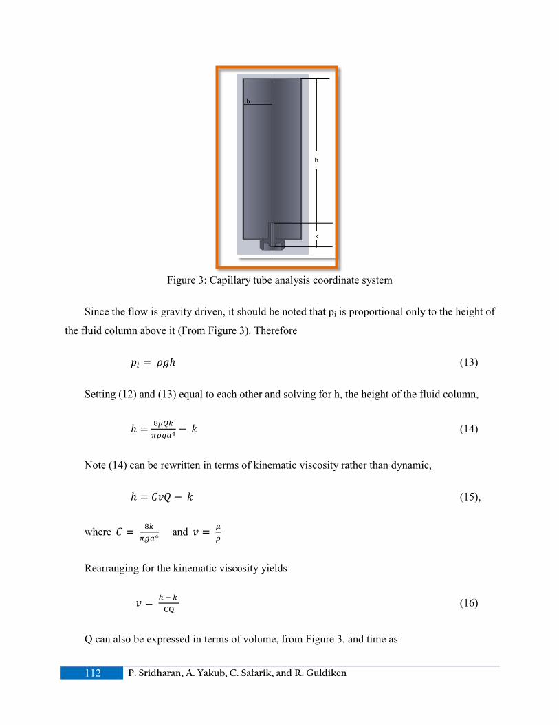
Figure 3: Capillary tube analysis coordinate system

Since the flow is gravity driven, it should be noted that pi is proportional only to the height of

the fluid column above it (From Figure 3). Therefore

𝑝𝑖 = 𝜌𝑔ℎ (13)

Setting (12) and (13) equal to each other and solving for h, the height of the fluid column,

ℎ = 8𝜇𝑄𝑘

𝜋𝜌𝑔𝑎4− 𝑘 (14)

Note (14) can be rewritten in terms of kinematic viscosity rather than dynamic,

ℎ = 𝐶𝑣𝑄 − 𝑘 (15),

where 𝐶 = 8𝑘

𝜋𝑔𝑎4 and 𝑣 = 𝜇

𝜌

Rearranging for the kinematic viscosity yields

𝑣 = ℎ + 𝑘

CQ (16)

Q can also be expressed in terms of volume, from Figure 3, and time as


𝑄 = 𝜋𝑏

2ℎ𝑡

(17)

Substituting (17) into (16) yields

𝑣 = ℎ + 𝑘

C𝜋𝑏2ℎ𝑡 (18)

(16) may also be rewritten in terms of the viscometer dimensions as

𝑣 = ��𝑔

8� (1

𝑏)2𝑎4 �1

𝑘+ 1

ℎ�� 𝑡 = 𝑀𝑡 (19),

where M is a constant. It is worth noting that (19) shows important insights into the sensitivity

of the function of the viscometer. The constant M is implicit and specific to each viscometer made,

which is dependent on the dimensions of the viscometer. Although M depends on the dimensions,

for proper calibration, the importance of each dimension must be known, such that each

dimension’s required tolerances can be assigned during manufacturing of the viscometer. (19) is

powerful in aiding with these insights.

It can be inferred from (19) that increasing or decreasing the capillary radius, a, exponentially

affects M since it is raised to the fourth power. Due to this, it can be seen that the capillary radius is

the most sensitive, and important, dimension of the viscometer in terms of its proper function. The

viscometer diameter, b, is the second most important dimension regarding the functioning of the

viscometer. It affects the function at an exponential rate, like capillary radius, but at a slower rate.

The lengths of the fluid column and capillary rank equally, but are last in line in dimensional

importance. Additionally, recalling from (15) about dynamic viscosity, (16) and (19) can be

rearranged as

𝜇 = 𝜌 ℎ + 𝑘

CQ= 𝜌𝜋𝑔𝑎

4(ℎ+𝑘)8𝑘𝑄

(20)

𝜇 = 𝜌 ��𝑔

8� (1

𝑏)2𝑎4 �1

𝑘+ 1

ℎ�� 𝑡 = 𝜌𝑀𝑡 (21),


113



where M is a constant. It is important to note that although, in terms of function of the

viscometer, the kinematic viscosity is not dependent on the density of the fluid, the relationship of

dynamic viscosity is density dependent. The kinematic viscosity mainly depends on the geometry

of the problem.

(a) (b)

Figure 4: Streamline Depictions of: (a) Bucket with hole in bottom and (b) viscometer; blue

indicates ~143 mm/s and yellow indicates ~36,800 mm/s velocity.

In addition to the above analysis, an elementary computational fluid simulation was done on

the tested viscometer. It is known that previous capillary viscometers existed, where the capillary tube started at the bottom of the cup, not offset in height, k, as in Figure 3. It was assumed that fluid flow accounted for this height offset. In other words, the reason for the height is assumed to be due to the streamlines of the flow during use. In order to test this theory we must visualize streamlines for different designs, and to get a general idea of how these streamlines change with the design. Therefore, a CFD (Computational Fluid Dynamics) model was done. A model of the viscometer was created using Solidworks. The FloExpress Simulation Module of Solidworks was used to run a fluids simulation to predict streamlines of flow. The simulation input required specifying an inlet and exit. The simulation required inlet conditions, while the outlet conditions were auto-set to be to open air at STP. The inlet conditions that were input was a volumetric flow rate and inlet pressure,


which were 10 in3/s, and 1 atm, respectively. The fluid was assumed be incompressible during the simulation, which was done through an iterated Navier-Stokes equation reduction. The first case considered was a tank with a hole at the bottom. The second case considered was the capillary viscometer. The result of this analysis is shown in Figure 4, where the color of the line corresponds to the speed of the flow; blue indicates lower speeds, whereas yellow indicate higher speeds.

Comparing the two pictures in Figure 4, it is easier to understand the reason for this height

offset. As can be seen in Figure 4a, the fluid that gets to the bottom of the tank undergoes turbulence as it transitions into the capillary hole. In addition to this turbulence, slight rotation in the flow can be seen as it enters the capillary. When looking at Figure 4b, lot of turbulence can also be seen. The difference is that turbulence occurs due to vortices developing on the sides of the capillary tube. These vortices occur in a way such that the turbulence does not affect the fluid entering the capillary tube. Another observation is that there is minimum rotation in the flow.

In effect, the transition the flow undergoes going from the viscometer into the capillary is a lot

smoother when the capillary is offset in height. This allows Assumptions 4 and 5 of the Capillary Tube Analysis to be more valid, causing the overall fluid analysis to have greater validity, causing higher accuracy of (19). It can also be seen from Figure 4b that the result from (3) seems viable since fully developed flow is depicted for most of the capillary tube. As an added case of support, the Reynolds Number was calculated for the capillary tube, using water as the fluid, which was 95. Note that this number is very low, so laminar flow is viable.

An interesting digress related to history is that Ford had a viscosity cup, Figure 5, which

attacked the previous problem in a different way (Wikipedia).

Figure 5: Ford Viscosity Cup (Wikipedia).


115



Notice the conical extrusion at the bottom of the cup. This conical profile allows the flow to

follow more of the streamline pattern as in Figure 4b. This ensures straight laminar entrance into

the capillary at the bottom. This method does have its disadvantages. Due to the profile of the

conical section, the fluid velocity accelerates as it gets near the outlet of the cup. This acceleration

may be more observable as angular rotation rather than laminar velocity. Although this does create

a stream tube as in 4b, there is a possibility of turbulence/angular rotation. The height offset as

shown in Figure 3 ensures a similar stream tube profile and also reduced chances of

turbulence/angular rotation.

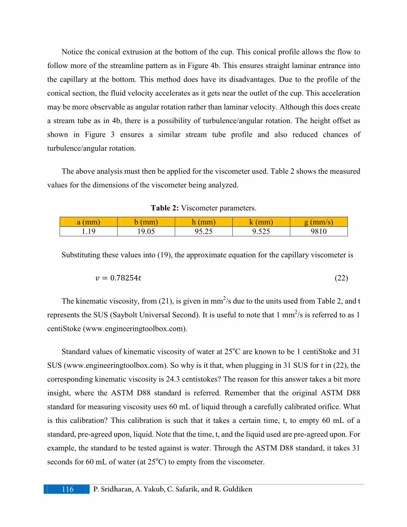
The above analysis must then be applied for the viscometer used. Table 2 shows the measured

values for the dimensions of the viscometer being analyzed.

Table 2: Viscometer parameters.

a (mm) b (mm) h (mm) k (mm) g (mm/s) 1.19 19.05 95.25 9.525 9810

Substituting these values into (19), the approximate equation for the capillary viscometer is

𝑣 = 0.78254𝑡 (22)

The kinematic viscosity, from (21), is given in mm2/s due to the units used from Table 2, and t

represents the SUS (Saybolt Universal Second). It is useful to note that 1 mm2/s is referred to as 1

centiStoke (www.engineeringtoolbox.com).

Standard values of kinematic viscosity of water at 25oC are known to be 1 centiStoke and 31

SUS (www.engineeringtoolbox.com). So why is it that, when plugging in 31 SUS for t in (22), the

corresponding kinematic viscosity is 24.3 centistokes? The reason for this answer takes a bit more

insight, where the ASTM D88 standard is referred. Remember that the original ASTM D88

standard for measuring viscosity uses 60 mL of liquid through a carefully calibrated orifice. What

is this calibration? This calibration is such that it takes a certain time, t, to empty 60 mL of a

standard, pre-agreed upon, liquid. Note that the time, t, and the liquid used are pre-agreed upon. For

example, the standard to be tested against is water. Through the ASTM D88 standard, it takes 31

seconds for 60 mL of water (at 25oC) to empty from the viscometer.


What would occur if the liquid being tested, whose viscosity is unknown, is very viscous, such that the time required for it to empty is very large (on orders of tens of minutes to hours)? What would occur if the liquid being tested is so inviscid, such that the time elapsed for emptying 60 mL is on the orders of few seconds, not long enough to gather data? Both of the above scenarios, which are encountered in larger frequency after the industrial revolution, would be hard to handle by one size of viscometer. Both of the above scenarios can be solved by changing the height of the fluid column, h, such that the time it took to empty that volume is kept in a second range that is workable out in the field/application. But changing the fluid column height also changes the volume of the fluid, causing it to differ from the traditional 60 mL, causing the test to not follow the ASTM standard.

This is actually not a real problem. The reason why is because of the nature of the definition of

viscosity, tied in with ASTM. The unit known as viscosity is not a physical unit. It is a theoretical unit which describes a physical presence, like gravity. This is the reason the ASTM D88 standard was created. Since viscosities of fluids greatly differ and difficult to define, a theoretical zero-bar is created, to which all other viscosities are related to. This zero-bar is through the ASTM D88 standard. Therefore the problem of changing the initial volume can be fixed if the time required for that volume to empty can be analogous for the time it takes for 60 mL to empty. Due to this, the relationship between units of kinematic viscosity (centistokes and SUS) is not related to the geometry of the viscometer, which is displayed in Figure 6. It is also interesting to note that the relationships in Figure 6 change depending on the temperature.

Figure 6: Centistoke to SUS conversion courtesy of "Standard Method for Conversion of Kinematic Viscosity to Saybolt Universal Viscosity or to Saybolt Furol Viscosity" ASTM

Standard 2161 (ANSI M9101).


117



It is also interesting to note that, using the values from Table 2, the volume of the fluid column in the viscometer tested is actually about 105 mL, not the standard 60 mL. The higher volume allows for a larger range of viscosities to be tested, but only if the fluids fall within a specific gravity range. But for this viscometer to work with 105 mL of initial volume and still relate to the standard, the capillary radius is calibrated. The capillary radius is changed because it has the highest effect on the function of the viscometer as discussed above. The capillary radius of the viscometer is properly calibrated if it takes 31 seconds for 105 mL of water to empty through this viscometer. Remembering that the time taken for discharge is the SUS (Saybolt Universal Second) value for that fluid, the relationships from Figure 6 hold to convert between centistoke and SUS.

The key thing to note from above is that (19) and (21) contain a constant, M, inherent to the

geometry of the viscometer. It is important to note that the constant depends on the dimensions of the viscometer. As long as the fluids being tested are within the specific gravity range of the viscometer's calibration, the constant M, from (19), also equals the ratio of kinematic viscosity, in centistokes, to kinematic viscosity, in SUS. This ratio is in accordance to the ASTM standard for conversion between SSU and Centistokes (ASTM D2161). For every SSU value, there is a corresponding Centistoke value at that temperature.

Therefore, for fluids with higher viscosities, the same capillary viscometer can be used, if the

dimensions are changed such that the stream tube of Figure 4b is valid, making the Navier-Stokes Derivation valid, in addition to proper time calibration. If a fluid is very viscous, just changing the fluid column height and the capillary radius to replicate the stream tube is not enough. In addition to above, it must be ensured that the time it takes for the fluid to empty is in accordance with analogous to the standard. If, by changing the height and capillary radius to account for the new fluid, the viscometer's new volume composed of water emptying through the new capillary radius does not equal 31 seconds (aka SUS), then all the times from the viscometer cannot be compared to the standard. The balance between the two previous sentences is what ensures proper calibration of the viscometer with assurance of proper functioning. It should be noted that the above is also only for distinct densities or density ranges.

3. Study Details The following fluids were tested: water, honey, dish detergent (Ajax), mixtures of water and

detergent; Car oils: SAE 5W-30, SAE 10W-30, SAE 10W-40, SAE 50W; Gear oil: SAE 75W-90.


These car/gear oils are engineered to have specific viscosities at two distinct temperatures during

operation. These temperatures are known as the cold start temperature and operation temperature.

The cold start temperature is the temperature at which the engine is turned on, which is also usually

when the oil is at its lowest temperature. The operation temperature is assumed to be 100 oC

(Celsius). Ambient temperature of 25 oC was chosen for simulating the cold start temperature due

to the fact that the temperature at which the engine is turned on can vary depending on altitude,

location, and other variables.

1. The following are procured: viscometer, stopwatch, fluids to be tested, containers, and a

gas flame.

2. The viscometer is cleaned thoroughly prior to each use.

3. A reservoir of liquid is heated over a gas flame, until the desired temperature is reached.

4. Once the fluid has become the desired temperature, the viscometer is submerged into the

fluid.

5. The viscometer is allowed to be submerged in the fluid to fill it up and held long enough to

ensure it, and the fluid, are at the desired temperature.

6. The viscometer is pulled out of the fluid; when the bottom face of the viscometer clears the

top of the liquid in the container, which allows the fluid to begin to fall out, the stopwatch is

started.

7. The liquid is allowed to empty from the viscometer.

8. The following times recorded from the stopwatch: start time, time at which flow change from stream to drips occurs, and time when liquid flow stops.

Note: If needed, multiple trials can be done for same liquid to average the times by repeating

Steps 2-8. During the procedure, the temperature of the liquid was monitored to ensure temperature

was constant.

The viscometer acquired for the analysis was designed for fuel oils. Most of these fuel oils

have a specific gravity range between 0.8-1.0 (www.engineeringtoolbox.com). Therefore,

preliminary testing was done with automotive car and gear oils, due to the fact that most

automotive oils have specific gravities between 0.88-0.94 (www.engineeringtoolbox.com). The


119



results of the experimental procedure are summarized in Table 3 below.

Table 3: Summary of Experimental Results.

Time (s) Oil Type 25 o Celsius 100 o Celsius

Stream to Drip Full Stop Stream to Drip Full Stop C: 5W-30 268 406 - 70 C: 10W-30 289 469 - 70 C: 10W-40 383 581 - 84

C: 50W - 1395 - 97 G: 75W-90 318 775 - 81

In Table 3, the column “Stream to Drip” represents the time at which the fluid flow out of the

viscometer changed from a steady stream to drips. The "C" or "G" before the oil type dictates

whether it is crankcase or gear oil. If the fluid flow never changes from a stream to drip, no time is

recorded. Whether the fluid drips or streams depends on the viscosity and surface tension of the

fluid. The column “Full Stop” is the overall time it took the volume of fluid to empty from the

viscometer. It is important to note that the Full Stop time at 100 oC corresponds to the kinematic

viscosity of the oil tested in Saybolt Universal Second. Car oils with an increasing number in

front of the W dictate an increase in viscosity. The physical representation of this can be inferred

from Table 1 since the Full Stop time increases as the number increases.

Table 4 shows the standard values (www.engineeringtoolbox.com), in SUS, of the oils tested

in Table 3. The values in Table 4 correspond to the Full Stop values at 100oC in Table 3. As seen

from Table 4, it is worth noting that the experimentally found kinematic viscosity, in SUS, of

car/gear oils tested is within 5% of the standard value.

Table 4: Standard Values of Car/Gear Oils.

Oil Type Standard Value @ 100oC (seconds)

C: 5W-30 70 C: 10W-30 70 C: 10W-40 85

C: 50W 110 G: 75W-90 74

The viscosities, at different temperatures, from Table 2 are in Figure 7.


Figure 7: Full Stop Time vs Temperature for Car/Gear oils.

Figure 8: ASTM Viscosity Chart.

0

500

1000

1500

25 100

Tim

e (s

econ

ds)

Temperature (⁰C)

C: 5W-30

C: 10W-30

C: 10W-40

G: 75W-90

C: 50W


121



It is well known that detergent is used in industry as a type of surfactant to change the surface

tension of fluids. A set of trials were done were concentration of detergent to water was varied in

different mixtures of dish detergent (Ajax) and water. The time required to empty the viscometer

(SUS) was tabulated for these, which is shown in Table 5. The purpose of these trials is to discern

some type of relationship between surface tension and viscosity of Ajax and/or Water. It seems that

Table 5: SUS values of Mixtures of Ajax and Water.

Ratio of Ajax to Water (%) Time (seconds)

0 31 8.3 40 16.7 40 25 41 50 43

62.5 49 75 52 88 3651

100 3780 A graphical representation of Table 5 is shown in Figures 9 and 10. Figure 10 is a close up of

first seven rows of Table 5, whose correlation is not discernible from Figure 9.

Figure 9: Ajax Mixture % vs Time.

Figure 10: Close up of 0-75% range from Figure 9.


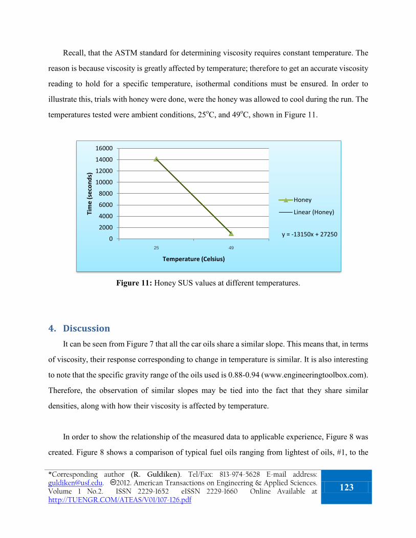
Recall, that the ASTM standard for determining viscosity requires constant temperature. The

reason is because viscosity is greatly affected by temperature; therefore to get an accurate viscosity

reading to hold for a specific temperature, isothermal conditions must be ensured. In order to

illustrate this, trials with honey were done, were the honey was allowed to cool during the run. The

temperatures tested were ambient conditions, 25oC, and 49oC, shown in Figure 11.

Figure 11: Honey SUS values at different temperatures.

4. Discussion It can be seen from Figure 7 that all the car oils share a similar slope. This means that, in terms

of viscosity, their response corresponding to change in temperature is similar. It is also interesting

to note that the specific gravity range of the oils used is 0.88-0.94 (www.engineeringtoolbox.com).

Therefore, the observation of similar slopes may be tied into the fact that they share similar

densities, along with how their viscosity is affected by temperature.

In order to show the relationship of the measured data to applicable experience, Figure 8 was

created. Figure 8 shows a comparison of typical fuel oils ranging from lightest of oils, #1, to the

y = -13150x + 27250 0

2000

4000

6000

8000

10000

12000

14000

16000

25 49

Tim

e (s

econ

ds)

Temperature (Celsius)

Honey

Linear (Honey)


123



heaviest, #6. It is important to note that the heaviest and most viscous fluid presented on the chart is

honey. In terms of specific gravities, the oils tested range between 0.88-0.94; water is

approximately 1; honey was measured to be approximately 2; pure Ajax was measured to be

approximately 0.8. Excluding honey, the specific gravity range for all liquids tested lie in the range

of 0.8-1 (within 20% of water). Although, from (21), the dynamic viscosity is density dependent,

Figure 6 shows wide range of viscosities corresponding to a small specific gravity range.

Making note of Figure 8, there is a narrow band of acceptable viscosity of 80 to 100 SUS

where a fuel oil must be heated in order to have clean combustion of the oil. Similarly the

accuracy of the fuel oil heating and circulation system has to maintain a fairly narrow range of

control. In other applications, such as paint spraying, coating etc. viscosity has to be accurately

controlled to prevent “orange peeling” or a wavy texture to the paint to enlarged droplet size.

Droplet size and fluid temperature are very dependent on one another.

As can be seen from Figures 9 and 10, the surfactant, dish detergent, does not affect the

viscosity of water as much as water affects the viscosity of it. It is interesting to note, that 100%

Ajax has an SUS value of approximately 3780. A decrease in concentration of just 15% decreases

the SUS value to 3619 (decrease of approximately 4.26% with respect to the value at 100% Ajax

concentration value). But a decrease of another 15% in Ajax concentration causes the SUS value to

decrease to 52 SUS., which is a decrease of approximately 98.6% of the 100% Ajax concentration

value.

Regarding Figure 11, the line named "Linear (Honey)" is a linear regression fitted to the

Honey data. The equation of this regression is shown on the Figure. We will use this equation to

extrapolate the viscosity of Honey (in SUS) at 100oC. Plugging in 100 for x in the equation, the

corresponding y (time aka SUS) comes out to -1,287,750 seconds. Obviously, this is incorrect. The

reason for this error is due to the Honey trial at 49oC. The time for the honey to empty is 950

seconds (15.8 minutes). During this time the honey decreased in temperature from 49oC at the start


of the trial to 32.2oC. The honey is very viscous, requiring the time for a given volume to empty to

increase. If insulation is not present, temperature of the honey will change, especially if the time

required for trial increases. This decrease in temperature causes a change in viscosity, since

viscosity is temperature dependent. Due to this reason, the data from the 49oC trial is very

erroneous, causing large errors in the linear regression. If the honey was well insulated, the linear

regression will be a better fit, giving a viable value when extrapolating to 100oC.

5. Conclusion It was found that of the main dimensions of the viscometer, the capillary radius and viscometer

radius greatly affected the performance of the viscometer compared to the fluid column height or

capillary tube height. The reason why the capillary tube was "inset" was found to help the transition

the fluid flow experiences going into the capillary tube. Creating the height offset minimized

turbulence and rotation of the flow entering the capillary tube. Constant temperature is essential to

the accuracy of the viscometer. Car/Gear oils were tested with the viscometer and all viscosity

results of the oils were with 5% of the real values.

Surface tension also was found to play a role in the viscometer. Once the surface tension force

is larger than the pressure force, in this case due to gravity, forcing the liquid down, the flow does

one of two things. If the flow was a steady stream out of the viscometer, it will either turn into

dripping flow and/or stop altogether. If the flow out of the viscometer was through drips to begin

with, the surface tension force then stops the flow of the fluid when it exceeds the pressure force.

6. References American Society for Testing and Materials (ASTM), 1972. Library of Congress Catalog Card

Number: 70-180913.


125



Hancock, Matthew J. and Bush, John W. (2002). Fluid Pipes. Journal of Fluid Mechanics, vol. 466, 285-304.

Prashanth Sridharan is currently pursuing his Doctorate Degree in Mechanical Engineering at University of South Florida, Tampa, Florida. Mr. Sridharan earned his Bachelor Degree in Mechanical Engineering from University of Florida in 2010. Current research interests include thermal science, alternative/renewable energy, and fluid dynamics.

Abiodun Yakub is an MS student in the Department of Mechanical Engineering at University of South Florida, Tampa, Florida. He earned his B. Tech. from Ladoke Akintola University of Technology (LAUTECH) Nigeria in 2004. Abiodun’s research interests include Dynamics and Material science.

Charles Robert Safarik, received his Bachelor of Science Degree in Aerospace Engineering from The Polytechnic Institute of New York, 1967, Masters in Mechanical Engineering, Pennsylvania State University, 1978, and currently studying for a Ph.D. in Mechanical Engineering at the University of South Florida. He was also a Registered Professional Engineer, Florida, from 1981- 2010, practicing in Heat Transfer and Combustion Design and Development.

Dr. Rasim Guldiken is an Assistant Professor in the Department of Mechanical Engineering at University of South Florida, Tampa, Florida. He earned his Ph.D. from Georgia Institute of Technology in 2008. Dr. Guldiken’s research interests include Microfluidics and Bio-MEMS.

Peer Review: This article has been internationally peer-reviewed and accepted for publication

according to the guidelines given at the journal’s website.




Fuzzy Logic Modeling Approach for Risk Area Assessment for Hazardous Materials Transportation Sanya Nameea, Boonsap Witchayangkoona*, Ampol Karoonsoontawongb

a Department of Civil Engineering, Faculty of Engineering, Thammasat University, THAILAND b Department of Civil Engineering, Faculty of Engineering, King Mongkut’s University of Technology Thonburi, THAILAND A R T I C L E I N F O

A B S T RA C T

Article history: Received 01 December 2011 Received in revised form 20 January 2012 Accepted 26 January 2012 Available online 28 January 2012 Keywords: Risk Area Assessment; Hazardous Material; Transportation; Fuzzy Logic Modeling.

The assessment of area in risk of HazMat transportation is very beneficial for the planning of the management of such area. We prioritized the affected area using HazMat-Risk Area Index (HazMatRAI) developed on the basis of Fuzzy Logic. The purpose of such development is to reduce limits of the criteria used for the assessment which we found exist when displaying data related to Hazmat represented by iceberg. In this regard, we categorized type of Membership Function according to Fuzzy set method in order to match the existing criteria, both solid and abstract ones. The conditions of Fuzzy Number and Characteristic are used respectively so that all risk levels are covered. However, the displaying of HazMat-Risk Area Index needs weighing of each criterion that is used for the assessment which significance of each level varies. We used Saaty’s Analytic Hierarchy Process (AHP) to establish weighing value obtained from such assessment. Therefore it is beneficial for the preparation of area with HazMatRAI value is high, hence proper preparation for the management in case of critical situation.


2012 American Transactions on Engineering & Applied Sciences

*Corresponding author (B.Witchayangkoon). Tel/Fax: +66-2-5643001 Ext.3101. E-mail address: [email protected]. 2012. American Transactions on Engineering & Applied Sciences. Volume 1 No.2 ISSN 2229-1652 eISSN 2229-1660. Online Available at http://TUENGR.COM/ATEAS/V01/127-142.pdf

127





1. Introduction Recently industrial sector has been growing rapidly. Industry involved with chemical

substances, nuclear, electrics, and petroleum are beneficial to the world, but at the same time they

come with complicated problems. These industries are generator where they need hazardous

material for the manufacturing process. Besides, some type of industry also produces hazardous

wastes. Major affects include the transportation of hazardous materials which occur everywhere in

pipe, rail, and road. It increases risk of people’s safety, life, property, and environment of the area

where transportation takes place. In the United States, we found that the transportation of

hazardous materials generates economic activities a great deal, for example, the transportation that

costs more than 2 billion dollars in the United States. Over all transportation increases to 20%

during 1997 – 2002 (USA Census Bureau, 2002) and transportation by truck is as high as 52.9%,

accidents on high way is 89%. For the accident, the serious ones are caused by the transportation of

hazardous material such as leaking or death, damage costs up to 31 billion dollars (about 80,000

dollars for 1 accident) (USA DOT, 2003). Despite our awareness that accident from hazardous

materials does not occur frequently (10-8 – 10-6 per vehicle per mile) (Erkut and Verter, 1995;

Zografos and Davis, 1989), the consequence is much to be concerned for every involved person or

everyone who is affected by the transportation of hazardous materials, involved people in the area,

government sector, transportation company, transportation vehicle, and people in risk. The

reduction of risk of transportation is the main purpose of every people involved in the

transportation of hazardous materials.

The National Fire Protection Agency (NFPA), 2008 has defined HazMat Risk that it is the

possibility and severity of sequence from the exposure to hazardous material. The result from this

definition is that the perception of hazardous material is always involved with leakage, and the

consequence of such leakage. Frequency of leakage depends on many factors e.g. possibility of

accident, possibility of leakage, and numbers of hazardous material transportation. Consequence

from the leakage depends on types of hazardous materials, amount of leakage, and duration from

the occurrence until the management. Hazardous material transportation can make people’s life

harmful, especially people who are living near transportation route. Besides, it also affects

environment. Although not frequent, if it occurs, it can lead to major disaster.

128 Sanya Namee, Boonsap Witchayangkoon, and Ampol Karoonsoontawong

Figure 1: The problem of hazardous material transportation is like an iceberg.

The inevitable truth in many countries is that the problem of hazardous material

transportation is like an iceberg. It is difficult to access the truth data about such transportation i.e.

pipe, rail, or road to see if it was operated with transparency. Avoidance and failure to comply to

the law, false information, ambiguous source of information, and the operation of officers that does

not cover all aspects, and the integration of involved units are all problems that have been hidden.

The preparation to handle the accident from hazardous material transportation plays an important

role in the safety of such transportation that results in the loss of life, property, and environment.

The major contributions of this paper are the guideline for the assessment of risk area from

hazardous materials using the theory of Fuzzy Set. The assessment is conducted under the

limitation of ambiguous factors in terms of both objective and subjective. Purpose of the

assessment is to obtain index for the identification of risk area from hazardous materials

2. Literature Review In the past, problems of route management were handled by the development of model for

solving problems using single or multiple criteria. Purpose of single criteria model is to identify

one route or one network that minimizes risk (Glickman, 1983; Batta and Chiu, 1988; Karkazis and

Boffey, 1995). Multiple criteria model refers to route management on the basis of expense such as

travel time, expense of transportation, risk of accident, estimated numbers of affected people, risk

Assessable problem

• Evidence-based statistic data is available • Specific responsible unit / organization

Problems difficult to assess

• Difficulty accessing data • Ambiguity of data source • Statistic data given is falsified • Integration of responsible units


129



of some special population group, and property damage (Zografos and Davis, 1989; McCoord and

leu, 1995; List and Turnquist, 1994). Route management and scheduling help us find out the

problems. In this regard, we need to identify travel time and the point that mitigation team has to

stop before reaching the scene (Cox, 1984; Cox and Turnquist, 1986; Nozick et al., 1997).

Research by Lassarre (1993) and lepofsky et al (1993) has explained the Decision Support System:

DSS covering the analysis of danger from transportation and accident management, identifying

following topics a) risk assessment on the basis of accident possibility, leakage, consequence, and

risk b) identify optimum route between two points on the basis of multiple criteria such as duration,

possibility of accident, and population in risk c) identification of the outcome from hazardous

material and the assessment of evacuation and the identification of existing road usage d) traffic

management on the affected scene.

Weigkricht and Fedra (1995) and Brainard et al (1996) introduced management of hazardous

material transportation route indicating the route between two points by using multiple criteria and

weighing. Coutinho – rodrigues et al (1997) introduced DSS for routing and positioning of rescue

team. Feature of DSS is the geographical display of the unaffected route for problem solving and

decision making. The system integrates various techniques for solving various problems. When

making consideration, users might create his/her own way of problem solving by changing weight

of expense under the decision or setting the lowest point to the highest point of expense. Frank et al

(2000) developed DSS to choose the route between origins to destinations, each point matched.

Criteria used for route selection includes population who are in risk and travel time. Erkut e al

(2007) discussed about the routing of hazardous material transportation that it is a very important

decision to reduce risk. To be specific, risk of hazardous material transportation can be

dramatically reduced if it is well planned i.e. selecting the route with least possibility of accident,

control consequence, and try to find the way to rescue without obstacles. Zografos and

Androutsopoulos (2008) studied supportive system for making decision about hazardous material

transportation and how to respond emergency situation, and scope of risk management includes

logistics for hazardous material and the decision to respond emergency situation. The developed

system can be applicable to a) the preparation of route selection for hazardous material

transportation with lowest expense and risk b) identification of rescue team that can access the

scene with minimum travel time and safety before service arrives c) finding out the route for rescue


team d) identification of the best evacuation plan. The developed system is used for the

management of hazardous material being transported in road network under the area of Thriasion

Pedion at Attica, Greece.

Research related to the study of criteria used for risk assessment includes Saccomanno and

Chan (1985). It introduced the model that let us see the consequence of accident towards

population. In face, this model needs two criteria which are minimum risk and minimum

possibility of accident. The third criteria is the economic aspect of problems such as expense of

truck. Zografos and Davis (1989) developed a method for making decision with multiple

objectives. The 4 objectives that were considered include I) population in risk II) property damage

III) expense of truck operation and IV) risk of expansion by establishing capacity of network

connecting point.

Leonelli et al (2000) developed optimum route using mathematical program for route

calculation. Result of the calculation is the selection of route that only reduces expense. Frand et al

(2000) developed spatial decision support system (SDSS) for selecting the route for hazardous

material transportation. GIS environment model has been developed to create route image, while a

mathematical program has also been set to evaluate the use of such route. The purpose of this

model is to reduce travel time between origin and destination. However the actual goal is to

emphasis on the limitation, travel time, possibility of accident on such route, involved population,

and risk of population, all of the mentioned help establish the limitation of this model. Risk of

population has been established by the possibility of accident, multiplied by number of population

in that area.

Most of the studies emphasis on the analysis of transportation route to find out the route with

minimum risk, and the importance has been given to road network with highest chance of accident.

In this study, we assess the risk of area that might be affected from hazardous material

transportation including piping system, railing system, and road network. The result from

assessment can identify level of risk of each area so that each area is able to get prepared for the

prevention of accident in an appropriate manner. *Corresponding author (B.Witchayangkoon). Tel/Fax: +66-2-5643001 Ext.3101. E-mail address: [email protected]. 2012. American Transactions on Engineering & Applied Sciences. Volume 1 No.2 ISSN 2229-1652 eISSN 2229-1660. Online Available at http://TUENGR.COM/ATEAS/V01/127-142.pdf

131



3. Fuzzy Set Theory Recently there has been an attempt to establish model and develop mathematical process for

solving problems of the system that is quite complicated including statistics, formula, or equation

that most fits to specific problem. Most engineering solution analyzes data in two ways that is

subjective and objective. General problem of engineering task is the necessity to manage uncertain

data i.e. uncertainty of numbers from the measurement or experiment, and the certainty of the

denotation. Fuzzy set theory is a new field of mathematical originated to handle subjective data. It

is accepted that it is a theory that can handle such problem properly.

The analysis for making decision regarding the area in risk of hazardous material

transportation for the management of disastrous situation under the certainty and limitation to data

access needs the analysis and decision making with multiple criteria. The main challenges of this

study are the consideration of criteria that might make the transportation harmful, either through

piping or railing system, road network, area categorization on the basis of Boolean Logic, and

evaluation limitation. Therefore we need to use Fuzzy Logic to solve problems that are still

ambiguous or unidentified. Besides, the process used for making decision can be implemented in

both quantitative and qualitative criteria, and some criteria are very outstanding.

The first person who introduced Fuzzy Set theory is Lofti A Zadeh, a professor of Computer of

California University, Berkley. He introduced his article regarding “Fuzzy Sets” (Zadeh L.A.,

1965). Zadeh defined fuzzy sets as sets whose elements have degrees of membership. Considered

sets are viewed in a function called Membership Function. Each member of the set is represented

by Membership Value which ranges between 0 – 1. When considering the Ordinary Sets, we found

that degree of membership of each set is represented by either value between 0 and 1, which means

no membership value at all, or complete value of membership respectively. Generally we found

that sometimes we cannot be so sure that something is qualified enough to be a member of that set

or not. We can see that fuzzy set theory if more flexible as partial membership is allowed in the set,

which is represented by degree, or the acceptance of change from being a non-member (0) until

being a complete member (1). Fuzzy Set theory (Zadeh L.A., 1965) leads to the idea of fuzzy

mathematics in various fields, especially in Electronic Engineering and Control that still uses the

fundamental of fuzzy set theory (Zadeh L.A., 1973). I hereby would like to mention fundamental

idea of fuzzy set, as mentioned by Zadeh, that fuzzy set can explain mathematics as follow:


According to the definition of fuzzy set that needs function of membership as a method to

establish qualification, fuzzy set A can by represented by member x, and membership degree of

such value as follow:

𝐴 = {(𝑥, 𝜇𝐴(𝑥))|𝑥 ∈ 𝑈} (1)

Given that U has degree of membership for A, following symbols are used:

𝐴 = ∫ 𝜇𝐴(𝑥)𝑈 𝑥� (2)

Fuzzy set A in Relative Universe (U) is set from characteristic by membership function

µA : U [0 , 1] i.e µA (x) is value of each member x in U which identifies grade of

membership of x in fuzzy set A. In this regard, fuzzy set is considered classical set or crisp set.

This Membership function is called characteristic function. For classical set, there are only 2

value which are 0 and 1 i.e. 0 and 1 represents non-membership, and membership in the set

respectively. The example of Figure 2 represents characteristic of Boolean set and fuzzy set. Here

we use “fuzzy set” to explain, which means the set defined in function (1) where A and B represent

any fuzzy set and U represents Relative Universe (U). We found that fuzzy set is different from

classical set because fuzzy set has no specific scope. Concept of fuzzy set facilitates the

establishment of framework that goes along with ordinary framework, but it is even more ordinary.

Fuzzy framework lets us have natural way to handle problems of uncertainty, which is involved

with the uncertainty of how to categorize membership, rather than random method.

4. The Risk Assessment Criteria The risk assessment of area with the consideration of piping system, railing system, and road is

a complicated process. Basically we need to consider many aspects including location, route

significance and geographical characteristics. Researches in the past used various tools for

assessment, which can be categorized as follow: safety, minimum travel time, minimum

transportation time, population in risk, environmental quality, and geographical characteristics as

shown in Table 1. When considered these factors, we have two topics that reflect the risk of area:

a) risk caused by various criteria used for the assessment and b) risk as a result from route *Corresponding author (B.Witchayangkoon). Tel/Fax: +66-2-5643001 Ext.3101. E-mail address: [email protected]. 2012. American Transactions on Engineering & Applied Sciences. Volume 1 No.2 ISSN 2229-1652 eISSN 2229-1660. Online Available at http://TUENGR.COM/ATEAS/V01/127-142.pdf

133



significance. In accordance to the assessment of risk are, we divided risk scale into 5 subsets as

follow

R = {R1, R2, R3, R4, R5} (3)

= {most risk, much risk, risk, less risk, least risk}

4.1 Membership Function Deviation To successfully use fuzzy set, it depends on appropriateness of membership function either

quantitative assessment or qualitative assessment, which can be used for the identification of

membership function. When considered the complication and ambiguous source of information,

we can use 2 types of membership function

Table 1: Assessment Criteria for the Area in Risk of Hazardous Material Transportation

Main-Criteria Sub-Criteria Membership Function Weight

Type of

transportation in

the area

Distance to transportation system if transported by road

Function I 0.045

0.062 Distance to transportation system if transported by rail

Function I 0.013

Distance to transportation system if transported by pipe Function I 0.004

Significance of

being a route for

HazMat

transportation

Transportation system to manufacturer / pier / industrial area is available in the area

Function II 0.027

0.040 Number of gas station available in transportation system

Function II 0.009

Transportation system available in the area that reduces distance / duration of transportation

Function II 0.004

Risk condition of

road in the area

Road characteristics that are risks of accident

Function II 0.027

0.131 Number of accidents occurred in the past

Function II 0.020

Number of Hazmat transportation trucks

Function II 0.084

Danger if

accident occurs

Distance to transportation system in case of explosion / fire

Function I 0.283 0.314

Distance to transportation system in case of leakage

Function I 0.031

Benefits of the

area

Characteristics of urban Function II 0.237

0.453 Population density Function II 0.173

Distance to town center Function I 0.043


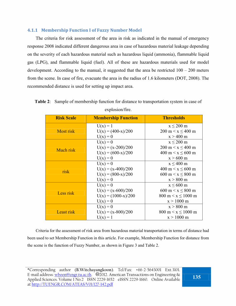
4.1.1 Membership Function I of Fuzzy Number Model

The criteria for risk assessment of the area in risk as indicated in the manual of emergency

response 2008 indicated different dangerous area in case of hazardous material leakage depending

on the severity of each hazardous material such as hazardous liquid (ammonia), flammable liquid

gas (LPG), and flammable liquid (fuel). All of these are hazardous materials used for model

development. According to the manual, it suggested that the area be restricted 100 – 200 meters

from the scene. In case of fire, evacuate the area in the radius of 1.6 kilometers (DOT, 2008). The

recommended distance is used for setting up impact area.

Table 2: Sample of membership function for distance to transportation system in case of

explosion/fire.

Risk Scale Membership Function Thresholds

Most risk U(x) = 1 U(x) = (400-x)/200 U(x) = 0

x ≤ 200 m 200 m < x ≤ 400 m

x > 400 m

Much risk

U(x) = 0 U(x) = (x-200)/200 U(x) = (600-x)/200 U(x) = 0

x ≤ 200 m 200 m < x ≤ 400 m 400 m < x ≤ 600 m

x > 600 m

risk

U(x) = 0 U(x) = (x-400)/200 U(x) = (800-x)/200 U(x) = 0

x ≤ 400 m 400 m < x ≤ 600 m 600 m < x ≤ 800 m

x > 800 m

Less risk

U(x) = 0 U(x) = (x-600)/200 U(x) = (1000-x)/200 U(x) = 0

x ≤ 600 m 600 m < x ≤ 800 m 800 m < x ≤ 1000 m

x > 1000 m

Least risk U(x) = 0 U(x) = (x-800)/200 U(x) = 1

x > 800 m 800 m < x ≤ 1000 m

x > 1000 m Criteria for the assessment of risk area from hazardous material transportation in terms of distance had

been used to set Membership Function in this article. For example, Membership Function for distance from

the scene is the function of Fuzzy Number, as shown in Figure 3 and Table 2.


135



Figure 2 Sample of Membership Function: Fuzzy Number

4.1.2 Membership Function II of Character

For Membership Function II of characteristics just like in Figure 3, generally it has

mathematical formula as follow

0 when x = Vi

U(x) = i = 1, 2, 3, …, m (4)

1 when x ≠ Vi

Characteristic Membership Function is seen as special type of fuzzy set. Actually normal

set can be used just like this. Or we can say that when U(x) has only point 0 and 1, fuzzy set will

automatically become non fuzzy set. In this research, characteristic function is used for the

assessment of risk area such as the area with transportation to manufacturer / pier / industrial area

in the area, and amount of hazardous material being transported. However they do not indicate

that there is a clear frame or it is difficult to check. Characteristic function will be used for the

cases that these data is not available, and it is difficult to establish characteristic function from the

assessment according to Membership Function I of Fuzzy Number. Therefore, the membership

function value has only 0 or 1. Regarding danger, it can be categorized into 5 levels as usual.

The estimation of involved amount of each criteria that uses Membership Function II for the

assessment makes us know that it can occur in 2 types which are i) amount and risk level with

direct variation and ii) amount and risk level with reverse variation, as shown in the Figure 3.

{


Figure 3: Sample of Characteristic Membership Function.

4.2 Weighting The assessment of risk area uses Saaty’s Analytic Hierarchy Process (AHP) to set weight of

each criteria related to the risk area. AHP is a mathematics method used for setting priority of each

criteria for making decision. The process consists of 3 parts which are identification and ordering,

assessment and comparison of elements in order, and integration using solution algorithm of

comparison result of every step. Scale for the comparison of priority (Huizingh and Virolijk, 1994)

consists of 9 levels of qualitative value: Equally Preferred, Equally to Moderately, Moderately

Preferred, Moderately to Strongly, Strongly Preferred, Strongly to Very Strongly, Very Strongly

Preferred, Very Strongly to Extremely, Extremely Preferred. Quantitative value had been set from

1 to 9 respectively. Calculation result from AHP is shown in Table 1.


137



5. Risk Assessment Model for Areas in Risk of Hazardous Materials

Transportation Developed from Fuzzy Sets We can see that there are 14 criteria for the assessment, as shown in Table 1. Each criteria is

different from each other and can be described as criteria set as follow:

M = {M1, M2,…. Mi, Mn}

Where Mi; i = 1, 2, 3, … n represents membership value of each risk area according to the

criteria used for assessment.

As mentioned in 4.2, each criteria has different significance which can be represented in form

of sets as follow:

W = {W1,W2,…. Wi, Wn}

Where Wi; i = 1, 2, 3 … n represents weight of criteria used in the assessment and size of

matrix is n x 1

To divide sets for decision making for the assessment of area R, it can be done as follow:

R = {R1, R2, ..., Rj, Rm}

Whereas Rj; j = 1, 2, .., m represents decision value of each level. Value of each risk set

consists of 5 levels including 0.9, 0.7, 0.5, 0.3, and 0.1 ranging from most risk to least risk and

matrix size is 1 x m

The area to be assessed has criteria data at i-th, which can be displayed in fuzzy matrix of M as

follow: M11 M12 . . . M1m

M21 M22 . . . M2m

Mij = . . . . . .

. . . Mij . .

. . . . . .

Mn1 Mn2 . . . Mnm

(Matrix 1)


Matrix displaying Mij shows membership value of the area to be assessed where i is in risk

level j

Matrix 1 with Mij is level of membership of area to be assessed of criteria i. It is a significant

model of how fuzzy is represented by data used for the assessment. Mij can be calculated using

membership value that is related to risk level. When combined with set of weight, the assessment to

find index value for the categorization of area in risk of hazardous material transportation will be

using model that uses set of R and M before going to weighing of each criteria with W.

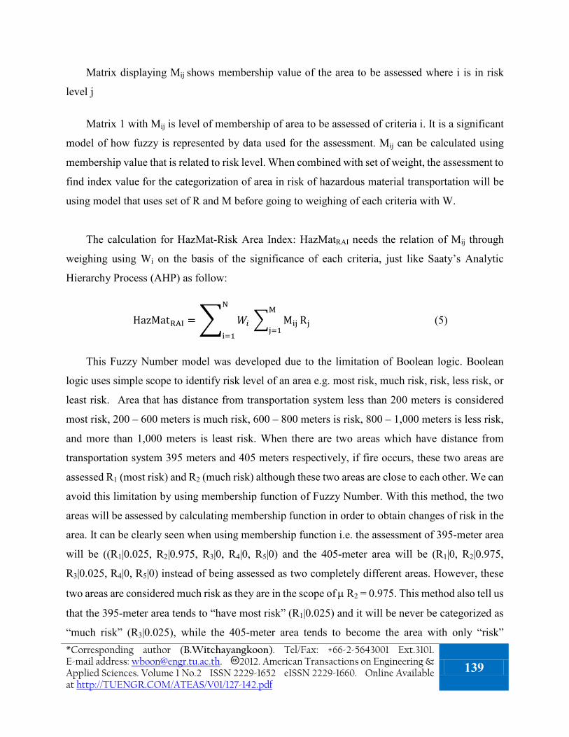
The calculation for HazMat-Risk Area Index: HazMatRAI needs the relation of Mij through

weighing using Wi on the basis of the significance of each criteria, just like Saaty’s Analytic

Hierarchy Process (AHP) as follow:

HazMatRAI = � 𝑊𝑖 � Mij

M

j=1Rj

N

i=1

(5)

This Fuzzy Number model was developed due to the limitation of Boolean logic. Boolean

logic uses simple scope to identify risk level of an area e.g. most risk, much risk, risk, less risk, or

least risk. Area that has distance from transportation system less than 200 meters is considered

most risk, 200 – 600 meters is much risk, 600 – 800 meters is risk, 800 – 1,000 meters is less risk,

and more than 1,000 meters is least risk. When there are two areas which have distance from

transportation system 395 meters and 405 meters respectively, if fire occurs, these two areas are

assessed R1 (most risk) and R2 (much risk) although these two areas are close to each other. We can

avoid this limitation by using membership function of Fuzzy Number. With this method, the two

areas will be assessed by calculating membership function in order to obtain changes of risk in the

area. It can be clearly seen when using membership function i.e. the assessment of 395-meter area

will be ((R1|0.025, R2|0.975, R3|0, R4|0, R5|0) and the 405-meter area will be (R1|0, R2|0.975,

R3|0.025, R4|0, R5|0) instead of being assessed as two completely different areas. However, these

two areas are considered much risk as they are in the scope of µ R2 = 0.975. This method also tell us

that the 395-meter area tends to “have most risk” (R1|0.025) and it will be never be categorized as

“much risk” (R3|0.025), while the 405-meter area tends to become the area with only “risk” *Corresponding author (B.Witchayangkoon). Tel/Fax: +66-2-5643001 Ext.3101. E-mail address: [email protected]. 2012. American Transactions on Engineering & Applied Sciences. Volume 1 No.2 ISSN 2229-1652 eISSN 2229-1660. Online Available at http://TUENGR.COM/ATEAS/V01/127-142.pdf

139



(R3|0.025) as well. We can clearly see changes of risk level when using membership function of

Fuzzy Number.

The calculation of HazMat-Risk Area Index (HazMatRAI) as mentioned above is the evaluation

of every criterion for weighing. It is reliable enough to be used for the assessment of area in risk of

hazardous material transportation, and it accommodates area diversity under the limitation of data

access. Such index can be used to identify risk level by making comparison of the calculated values

as HazMatRAI that uses comparison of related value ranging from biggest one to smallest one.

6. Conclusion Planning for the management of disaster caused by hazardous material transportation needs to

pay much attention to transportation system. This study has established criterions for the

assessment of area in risk and it covers all land transportation, with most emphasis on road. We

found that transportation by road has more risk of accident than other systems. However facts

about areas in risk of hazardous material transportation are rare and difficult to access. that’s why

the analysis cannot be done clearly. Using Fuzzy Set for the assessment of both objective and

subjective criteria is another way to develop model in order to obtain value that can be used in the

comparison of risk in the area. Literature reviews and relevant researches tell us that criterions used

for the assessment always emphasis on transportation by car and route network. Implementation of

study result has much effect towards the management of disaster for the local authority, including

the planning for establishment of HazMat team.

Result obtained from Fuzzy Set model is HazMat-Risk Area Index (HazMatRAI) which is used

to identify value of such area. Besides it can be used for comparison of risk level ranging from

biggest one to smallest one.

The next step of model development is to find the value of HazMat-Risk Area Index. In this

regard, many things can be done such as establishing weighing value of each criteria using various

expertise to establish such weighing value. Besides, the establishment of membership level of each

objective criteria can use Geographic Information System (GIS) to help categorize in order to

display geographical data more clearly. However, the idea of this study is to support decision

making for the assessment under ambiguous context in an appropriate manner.


7. References Batta, R. and Chiu, S.S., 1988 Optimal obnoxious parts on a network: transportation of hazardous

materials. Operation Research 36.

Carlsson, C., Fedrizzi, M. and Fuller R., 2004. Fuzzy Logic in Management. United States. Kluwer Academic Publishers.

Cox, E.G., 1984. Routing and scheduling of hazardous materials shipments: algorithmic approaches to managing spent nuclear fuel transport. Ph.D. Dissertation, Cornell University, Ithaca, New York.

Cox, E.G. and Turnquist. M.A., 1986. Scheduling truck shipments of hazardous materials in the presence of curfews. Transportation Research Record 1063.

Department of Transport, 2008. Emergency Response Guidebook, United States.

Devlin, Edward S., 2007. Crisis Management Planning and Execution. New York: Taylor & Francis Group.

Ghada, M.H., 2004 Risk Base Decision Support Model for Planning Emergency Response for Hazardous Material Road Accidents. Ph.D. Dissertation. The University of Waterloo. Ontario. Canada.

Glickman, T.S., 1983. Rerouting railroad shipments for hazardous material to avoid populated area. Accident Analysis Prevention 15.

Hazarika, S., 1987. Bhopal: The lessons of a tragedy. Penguin Book. New Delhi.

Jensen, C. Delphi in Depth., 1996. Power Techniques from the Experts Berkley. Singapore McGraw-Hill.

Karkazis, J. and Boffey, B., 1995. Optimal location of routes for vechicles transporting hazardous materials. European Journal of operational Research (86/2).

Lapierre, D. and Moro, J., 2002. Five Past Midnight in Bhopal. Warner Books. New York

List, G. and Turnquist, M., 1994. Estimating truck travel pattern in urban areas. Transportation Research Record 1430.

McCord, M.R. and Leu. A.Y.C., 1995. Sensitivity of optimal hazmat routes to limited preference specification. Information Systems and Operational Research (33/2).

Moore, D.A., 2004. The new risk paradigm for chemical process security and safety. Journal of Hazardous Material.

Mould, R. F., 2002. Chernobyl Record: The definitive history of the Chernobyl catastrophe. *Corresponding author (B.Witchayangkoon). Tel/Fax: +66-2-5643001 Ext.3101. E-mail address: [email protected]. 2012. American Transactions on Engineering & Applied Sciences. Volume 1 No.2 ISSN 2229-1652 eISSN 2229-1660. Online Available at http://TUENGR.COM/ATEAS/V01/127-142.pdf

141



National Fire Protection Association, 2001. Code and Standard- Massachusetts United States. Available from :(http://www.nfpa.org) Access November 2008

Sikich, Geary W., 1996. “All Hazards” Crisis Management Planning. Highland: Pennwell Books.

Smith, D., 2005. What ‘s in a name? The nature of crisis and disaster-a search for Signature qualities. Working Paper. University of Liverpool Science Enterprise Centre. Liverpool.

Zadeh, L.A., 1965. Fuzzy Sets. Information and control, Vol.8

Zografos, K.G. and Androutsopoulos. K.N., 2008. A decision support system for integrated hazardous materials routing and emergency response decisions. Transportation Research Part C 16.

Zografos, K.G. and Davis C.F., 1989 A multiobjective programming approach for routing hazardous materials. ASCE Transportation Engineering Journal (115/6).

S. Namee is currently a PhD candidate in Department of Civil Engineering at Thammasat University. He has been working at the Department of Disaster Prevention and Mitigation, Ministry of Interior, THAILAND. His research interests encompass hazardous material transport.

Dr. B. Witchayangkoon is an Associate Professor of Department of Civil Engineering at Thammasat University. He received his B.Eng. from King Mongkut’s University of Technology Thonburi with Honors in 1991. He continued his PhD study at University of Maine, USA, where he obtained his PhD in Spatial Information Science & Engineering. Dr. Witchayangkoon current interests involve applications of emerging technologies to engineering.

Dr. A. Karoonsoontawong is an Assistant Professor of Department of Civil Engineering at King Mongkut’s University of Technology Thonburi. He received his B.Eng. from Chulalongkorn University with Honors in 1997. He received his M.S. and Ph.D. in Transportation Engineering in 2002 and 2006, respectively, from The University of Texas at Austin, USA. Dr. Ampol is interested in transportation network modeling, logistical distribution network optimization, and applied operations research.




http://www.nfpa.org/faq.asp?categoryID=928&cookie%5Ftest=1



Computer Modeling of Internal Pressure Autofrettage Process of a Thick-Walled Cylinder with the Bauschinger Effect Zhong Hua*, and Sudhir Puttaguntaa

a

Department of Mechanical Engineering, South Dakota State University, USA A R T I C L E I N F O

A B S T RA C T

Article history: Received January 13, 2012 Accepted January 27, 2012 Available online January, 28 2012 Keywords: Thick-walled cylinder; Internal Pressurize; Autofrettage; Bauschinger effect; Finite Element Analysis

In this paper, the internally pressure overloading autofrettage process of a thick-walled cylinder has been numerically investigated. The corresponding axi-symmetric and plane-stress finite element model has been employed. The elasto-plastic material model with nonlinear strain-hardening and kinematic hardening (the Bauschinger effect) was adopted. The residual stresses in the thick-walled cylinder induced by internal autofrettage pressure have been investigated and optimized. The optimum autofrettage pressure and the maximum reduction percentage of the von Mises stress in the autofrettaged thick-walled cylinder under the elastic-limit working pressure have been found, the differences of stress and strain distribution between adopting the Bauschinger-effect and the non-Bauschinger-effect have been compared.


1. Introduction Thick-walled cylinders subjected to high internal pressure and/or elevated temperature are

widely used in the nuclear and chemical industries involving pressures as high as 1380 MPa and


*Corresponding author (Z.Hu). Tel/Fax: +1-605-688-4817. E-mail address: [email protected]. 2012. American Transactions on Engineering & Applied Sciences. Volume 1 No.2 ISSN 2229-1652 eISSN 2229-1660. Online Available at http://TUENGR.COM/ATEAS/V01/143-161.pdf

143





temperatures of up to 300 °C, (Ford et al. 1981) especially for military applications involving

transient peak internal pressures as high as 350 MPa and temperature of up to 1500 °C inside the

gun barrel in a ballistic event. (Bundy et al. 1996) In the absence of residual stresses, cracks usually

form at the bore where the hoop stress developed by the working pressure is highest. (Daniels

1942; Zapfec 1942; Bush 1988; Masu and Graggs 1992) To prevent such failure and to increase the

pressure-carrying capacity, a common practice is autofrettage treatment of the cylinder prior to use.

Autofrettage is used to introduce advantageous favorable compressive residual hoop stress inside

wall of a cylinder and result in an increase in the fatigue lifetime of the component. There are

basically three types of autofrettage. These are carried out by hydraulic pressurization, by

mechanically pushing an oversized mandrel, or by the pressure of powder gas, (Davidson and

Kendall 1970; Malik and Khushnood 2003) in which hydraulic and powder gas pressurization are

based on the same principal and strengthening mechanism. In general, vessels under high pressure

require a strict analysis for an optimum design for reliable and secure operational performance.

Prediction of residual stress field and optimization of the autofrettage processes’ parameters are

some of the key issues in this context, which normally involve a careful evaluation of the related

modeling, simulation and experimental details. (Davidson et al. 1963; Chu and Vasilakis 1973;

Shannon 1974; Tan and Lee 1983; Gao 1992; Avitzur 1994; Kandil 1996; Lazzarin and Livieri

1997; Zhu and Yang 1998; Venter et al. 2000; Gao 2003; Iremonger and Kalsi 2003; Kihiu et al.

2003; Parker et al. 2003; Perry and Aboudi 2003; Zhao et al. 2003; Perl and Perry 2006; Bihamta et

al. 2007; Hojjati and Hassani 2007; Korsunsky 2007; Gibson 2008; Perry and Perl 2008; Ayob et

al. 2009; Darijani et al. 2009) Efforts are continually made in the regarding aspects. Overloading pressure autofrettage process involves the application of high pressure to the

inner surface of a cylinder, until the desired extent of plastic deformation is achieved. Analytical

solution of pressure autofrettage of a constant cross-section cylinder, subject to some end

conditions, is possible through the use of simplifying assumptions, such as choice of yield criteria

and material compressibility and, critically, material stress-strain behavior. On the other hand,

autofrettage causes large plastic strains around the inner surface of a cylinder, which noticeably

causes the early onset of non-linearity when remove the autofrettage pressure in the unloading

process – a kinematic hardening phenomenon termed the Bauschinger effect. This non-linearity

typically causes significant deviation from those material models that are often assumed. The effect

is most pronounced around the inner surface, and in turn has a significant effect on the residual

144 Zhong Hu, and Sudhir Puttagunta

stresses developed when the autofrettage load is removed, especially as it can cause reverse

yielding to occur when it otherwise would not be expected. Research has been done on this issue

with theoretical analysis mostly based on bilinear kinematic hardening (linear elastic and linear

hardening) material model which is a good approximation for small strain. (Lazzarin and Livieri

1997; Venter et al. 2000; Kihiu et al. 2003; Parker et al. 2003; Perry and Aboudi 2003; Huang 2005;

Perl and Perry 2006; Korsunsky 2007). However, the practical material model is of nonlinear

kinematic hardening and with equivalent strain up to 0.5~1% in the autofrettage process, which

gives complexity to theoretical analysis using nonlinear kinematic hardening material model. In

this paper, the internally pressure overloading autofrettage process will be numerically

investigated. An axi-symmetric and plane stress (for open-ended cylinder) finite element model

will be presented. The elasto-plastic nonlinear material constitutive relationship will be adopted,

incorporating a nonlinear kinematic hardening (the Bauschinger effect) for which no analytical

solution exists. The effects of the autofrettage pressure on the residual stresses in a thick-walled

cylinder will be evaluated. The percentage of stress reduction by autofrettage treatment will be

calculated based on von Mises yield criterion. The optimum autofrettage pressure will be found.

The differences of stress and strain distribution between adopting the Bauschinger-effect and the

non-Bauschinger-effect will be compared.

2. Mathematical Model In this work, the thick-walled cylinder is made of stainless steel AISI 304. An elasto-plastic

governing equations for material behavior with a homogeneous and isotropic hardening model is

used. The true stress – true strain behavior of the strain hardening material follows the Hooke’s law

in the elastic region, and, for comparison purpose, the power-law hardening in the plastic region,

(Hojjati and Hassani 2007)

𝜎𝜎 = �𝐸𝐸𝐸𝐸 𝐸𝐸 < 𝐸𝐸𝑦𝑦𝐾𝐾𝐸𝐸𝑛𝑛 𝐸𝐸 ≥ 𝐸𝐸𝑦𝑦

(1),

where σ and 𝐸𝐸 are true stress and true strain, respectively. 𝐸𝐸𝑦𝑦 is the strain at the yield point. E is

the modulus of elasticity. K is a material constant equal to 𝐾𝐾 = 𝜎𝜎𝑦𝑦𝐸𝐸𝑦𝑦−𝑛𝑛 = 𝜎𝜎𝑦𝑦1−𝑛𝑛𝐸𝐸𝑛𝑛, and n is the

strain-hardening exponent of the material (0 ≤ n < 1). σy is the yield stress. Table 1 lists the basic


145



parameters and material data and derived material parameters to be used in the FEA modeling. (Peckner and Bernstein 1977; Harvey 1982; Boyer et al. 1985; ASM International Handbook Committee 1990). Figure 1 shows the elasto-plastic stress-strain relationship with kinematic hardening (the Bauschinger effect). Commercially available software ANSYS has been used for finite element modeling of the autofrettaged thick-walled cylinder. (Swanson Analysis System Inc. 2011) The finite element model is shown in Figure 2. The element PLANE183 with the capacity of elastic and plastic material nonlinearity and non-linear kinematic hardening (the Bauschinger-effect) has been adopted, which is an eight-node plane-stress 2-D element with higher accuracy quadratic shape function. In order to get reasonable accuracy, more elements are used near inner surface and outer surface of the cylinder, see Figure 2.

Table 1: Model dimensions and material properties.

Material of the Cylinder AISI304 Modulus of Elasticity E 196.0 GPa Poisson's Ratio υ 0.29 Yield Strength 𝜎𝜎𝑦𝑦 152.0 MPa* Strain at Yield Point 𝐸𝐸𝑦𝑦 7.755×10-4 Strain-Hardening Exponent n 0.2510 Material Constant K 917.4 MPa Inner Radius a 60 mm Outer Radius b 90 mm Maximum Working Pressure pi 47.22MPa

* corresponding to 215MPa at 0.2% offset and ultimate tensile strength of 505 MPa.

Figure 1: The elasto-plastic stress – strain model with kinematic hardening (the Bauschinger

effect).


Figure 2: Finite element model of a plane-stress thick-walled cylinder.

3. Modeling Results and Discussions Consider a thick-walled cylinder having inner radius a and outer radius b and subjected to the

internal pressure pi as shown in Figure 2. The material will obey the Hooke’s law when it is within

the elastic region. This allow us to use the Lame’s equations for calculating the hoop stress, 𝜎𝜎𝜃𝜃, and

radial stress, 𝜎𝜎𝑟𝑟, along the thickness of the cylinder, when the ends of the cylinder are open and

unconstrained so that the cylinder is in a condition of plane stress. (Ugural 2008)

𝜎𝜎𝜃𝜃 = 𝑎𝑎2𝑝𝑝𝑖𝑖𝑏𝑏2−𝑎𝑎2

�1 + �𝑏𝑏2

𝑟𝑟2�� (2),

𝜎𝜎𝑟𝑟 = 𝑎𝑎2𝑝𝑝𝑖𝑖𝑏𝑏2−𝑎𝑎2

�1 − �𝑏𝑏2

𝑟𝑟2�� (3),

𝜎𝜎𝑧𝑧 = 0 (4),

Therefore, the von Mises (equivalent) stress is

𝜎𝜎𝑖𝑖 = �𝜎𝜎𝜃𝜃2 + 𝜎𝜎𝑟𝑟2 − 𝜎𝜎𝜃𝜃𝜎𝜎𝑟𝑟�12 = 𝑎𝑎2𝑝𝑝𝑖𝑖

𝑏𝑏2−𝑎𝑎2�1 + 3 �𝑏𝑏

𝑟𝑟�4�12 (5),

The radial displacement is


147



𝑢𝑢 = 𝑎𝑎2𝑝𝑝𝑖𝑖𝑟𝑟𝐸𝐸(𝑏𝑏2−𝑎𝑎2) �(1 − 𝜈𝜈) + (1 + 𝜈𝜈) 𝑏𝑏

2

𝑟𝑟2� (6),

Obviously, the maximum von Mises stress is at r = a. Assuming von Mises yield criterion

applied, i.e., 𝜎𝜎𝑖𝑖 ≤ 𝜎𝜎𝑦𝑦, so by substituting the data from Table 1, the maximum applied working

pressure (the maximum internal pressure without causing yielding) is

𝑝𝑝𝑤𝑤𝑚𝑚𝑎𝑎𝑚𝑚 = 𝜎𝜎𝑦𝑦𝑏𝑏2−𝑎𝑎2

𝑎𝑎2�1 + 3 �𝑏𝑏

𝑎𝑎�4�−12

= 47.2 (MPa) (7),

Figure 3 shows the analytical and modeling results of stress components and radial

displacement along the thickness of the cylinder subjected to the maximum working pressure (pw

max = 47.2 MPa). The modeling results are well agreed with the analytical results from Lame’s

equations, indicating the reliability of the model employed in the numerical analysis. Figure 3 also

shows that the maximum von Mises stress and hoop stress located at the inner surface of the

cylinder, and the hoop stress is the major stress component causing yield failure.

Figure 3: Analytical and modeling results of stresses and radial displacement along the thickness

of the cylinder subjected to the maximum working pressure (pw max = 47.2 MPa).

3.4E-5

3.5E-5

3.6E-5

3.7E-5

3.8E-5

3.9E-5

4.0E-5

4.1E-5

4.2E-5

-0.4

-0.2

0

0.2

0.4

0.6

0.8

1

1.2

0 20 40 60 80 100

Stre

ss R

atio

σ/σ

y

(r-a)/(b-a)×100 (%)

σθ/σy by Eq.(2) σθ/σy by Modeling σr/σy by Eq.(3) σr/σy by Modeling σi /σy by Eq.(5) σi/σy by Modeling u by Eq.(6)

Disp

lace

men

t u

(m)


Figure 4: The relationship of elastic-plastic interface ρ and the autofrettage pressure pa.

As the internal pressure increasing, yielding (plastic deformation) starts from cylinder’s inner

surface and gradually extends towards cylinder’s outer surface. This process is basically an

elastic-plastic deformation process. The relation between internal autofrettage pressure, pa, and the

radius of the elastic-plastic boundary (interface) in plane stress condition, ρ, is determined by (Gao

1992; Gao 2003)

⎩⎪⎪⎨

⎪⎪⎧𝑝𝑝𝑎𝑎𝜎𝜎𝑦𝑦

= 2√3�cos�𝜑𝜑𝜌𝜌+𝜑𝜑𝑛𝑛�cos(𝜑𝜑𝑎𝑎+𝜑𝜑𝑛𝑛)�

�3𝑛𝑛2+𝑛𝑛��3𝑛𝑛2+1� 𝑒𝑒𝑒𝑒𝑝𝑝 �√3𝑛𝑛(𝑛𝑛−1)

3𝑛𝑛2+1�𝜑𝜑𝑎𝑎 − 𝜑𝜑𝜌𝜌�� cos𝜑𝜑𝑎𝑎 ,

𝜌𝜌 = 𝑎𝑎�sin(𝜑𝜑𝑎𝑎+𝜋𝜋/6)sin�𝜑𝜑𝜌𝜌+𝜋𝜋/6�

�cos�𝜑𝜑𝜌𝜌+𝜑𝜑𝑛𝑛�cos(𝜑𝜑𝑎𝑎+𝜑𝜑𝑛𝑛)�

2𝑛𝑛�3𝑛𝑛2+1� 𝑒𝑒𝑒𝑒𝑝𝑝 �√3

21−𝑛𝑛2

3𝑛𝑛2+1�𝜑𝜑𝜌𝜌 − 𝜑𝜑𝑎𝑎�� ,

𝜑𝜑𝜌𝜌 = cos−1 �√32

�𝑏𝑏2−𝜌𝜌2��3𝑏𝑏4+𝜌𝜌4

� ,

(8),

Where

𝜑𝜑𝑛𝑛 = cos−1 � √3𝑛𝑛√3𝑛𝑛2+1

� (9),

During autofrettage process, the elastic-limit pressure pe (pressure at which yielding

commences at inner surface) is obviously 𝑝𝑝𝑒𝑒𝑝𝑝𝑤𝑤 𝑚𝑚𝑎𝑎𝑚𝑚

= 1 and 𝜌𝜌 = 𝑎𝑎 in the given case, and the

plastic-limit pressure py (pressure at which plasticity has spread throughout the cylinder) is

1

1.1

1.2

1.3

1.4

1.5

1.6

0 20 40 60 80 100

Auto

fret

tage

Pre

ssur

e Ra

tio

p a/p

wm

ax

Elasto-plastic interface (ρ-a)/(b-a)*100 (%)

pa/pw max by Eq.(8) from Refs. (Gao1992 and 2003)pa/pw max by Modeling


149



𝑝𝑝𝑦𝑦𝑝𝑝𝑤𝑤 𝑚𝑚𝑎𝑎𝑚𝑚

= 1.543 and 𝜌𝜌 = 𝑏𝑏 in the given case. Figure 4 shows the relation of elastic-plastic interface

ρ and the autofrettage pressure pa obtained by modeling and analytical approaches, they are well

agreed.

Figures 5-7 show the autofrettage stress distributions for the thick-walled cylinder subjected to

different internal autofrettage pressure range of 𝑝𝑝𝑎𝑎𝑝𝑝𝑤𝑤 𝑚𝑚𝑎𝑎𝑚𝑚

= 1~1.6 by modeling. Hoop stress and

von Mises stress in Figures 5 and 7 clearly indicate that by increasing applied autofrettage pressure,

elastic-plastic interface (the turning point of the curve corresponding to the position ρ in Figure 4)

moves towards the outer surface of the cylinder and eventually reaches the outer surface, while

radial stress in Figure 6 indicate that the radial stress in compression, with highest compressive

stress in the inner surface and zero in the outer surface, increasing as the autofrettage pressure

increasing.

Figure 5: Autofrettage hoop stress distribution under different autofrettage pressure.

0.4

0.5

0.6

0.7

0.8

0.9

1.0

1.1

0 20 40 60 80 100

Auto

fret

tage

Hoo

p St

ress

Rat

io σ

a θ/σy

(r-a)/(b-a)*100 (%)

by Modeling under pw maxby Modeling under 1.1 pw maxby Modeling under 1.2 pw maxby Modeling under 1.3 pw maxby Modeling under 1.4 pw maxby Modeling under 1.5 pw maxby Modeling under 1.6 pw max


Figure 6: Autofrettage radial stress distribution under different autofrettage pressure.

Figure 7: Autofrettage von Mises stress distribution under different autofrettage pressure.

-0.50

-0.45

-0.40

-0.35

-0.30

-0.25

-0.20

-0.15

-0.10

-0.05

0.000 20 40 60 80 100

Auto

fret

tage

Rad

ial S

tres

s Rat

io σ

a r/σy

(r-a)/(b-a)*100 (%)

by Modeling by pw maxby Modeling under 1.1 pw maxby Modeling under 1.2 pw maxby Modeling under 1.3 pw maxby Modeling under 1.4 pw maxby Modeling under 1.5 pw maxby Modeling under 1.6 pw max

0.4

0.6

0.8

1.0

1.2

1.4

0 20 40 60 80 100

Auto

fret

tage

von

Mis

es S

tres

s Rat

io σ

a i/σy

(r-a)/(b-a)*100 (%)

by Modeling under pw maxby Modeling under 1.1 pw maxby Modeling under 1.2 pw maxby Modeling under 1.3 pw maxby Modeling under 1.4 pw maxby Modeling under 1.5 pw maxby Modeling under 1.6 pw max


151



When the internal autofrettage pressure is removed, the elastic deformation is trying to resume

its original shape while the plastic deformation is resisting this process so that residual stresses

within the cylinder have been induced, and the so-called pressure autofrettage process has been

accomplished. This unloading process basically is treated elastically. However, reverse yielding is

possible if earlier onset happens due to the Bauschinger effect. Figures 8-10 show the residual

stress distribution after removed autofrettage pressure. From Figure 8, it shows a compressive

residual hoop stress near the inner surface generated which is favorable to the thick-walled cylinder

when it is under internal working pressure (partially cancelling the tensile hoop stress induced by

the working pressure), and a tensile residual hoop stress near the outer surface of the cylinder.

Figure 9 shows a relative smaller but compressive residual radial stress left inside of the thick-wall,

satisfying the boundary conditions of zero radial stress on inner surface and outer surface of the

cylinder. Figure 10 shows the residual von Mises stress with higher values basically near the inner

surface and outer surface of the cylinder. The turning points of the curves in Figures 8 and 10 are

almost the same as in Figures 5 and 7 indicates that the earlier onset of the reverse yielding is very

less, not changing the elastic-plastic interface very much.

Figure 8: Residual hoop stress distribution after removed the autofrettage pressure.

-0.4

-0.3

-0.2

-0.1

0.0

0.1

0.2

0.3

0 20 40 60 80 100

Resi

dual

Hoo

p St

ress

Rat

io σ

r θ/σy

(r-a)/(b-a)*100 (%)

by Modeling with autofrettage of 1.1 pw maxby Modeling with autofrettage of 1.2 pw maxby Modeling with autofrettage of 1.3 pw maxby Modeling with autofrettage of 1.4 pw maxby Modeling with autofrettage of 1.5 pw maxby Modeling with autofrettage of 1.6 pw max


Figure 9: Residual radial stress distribution after removed the autofrettage pressure.

Figure 10: Residual von Mises stress distribution after removed the autofrettage pressure.

-0.05

-0.04

-0.03

-0.02

-0.01

0.00

0.01

0 20 40 60 80 100

Resi

dual

Rad

ial S

tres

s Rat

io σ

r r/σy

(r-a)/(b-a)*100 (%)


0.00

0.05

0.10

0.15

0.20

0.25

0.30

0.35

0.40

0 20 40 60 80 100

Resi

dual

von

Mis

es S

tres

s Rat

io σ

r i/σy

(r-a)/(b-a)*100 (%)



153



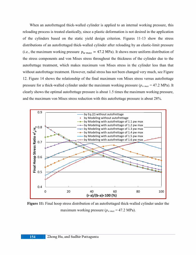
When an autofrettaged thick-walled cylinder is applied to an internal working pressure, this

reloading process is treated elastically, since a plastic deformation is not desired in the application

of the cylinders based on the static yield design criterion. Figures 11-13 show the stress

distributions of an autofrettaged thick-walled cylinder after reloading by an elastic-limit pressure

(i.e., the maximum working pressure 𝑝𝑝𝑤𝑤 𝑚𝑚𝑎𝑎𝑚𝑚 = 47.2 MPa). It shows more uniform distribution of

the stress components and von Mises stress throughout the thickness of the cylinder due to the

autofrettage treatment, which makes maximum von Mises stress in the cylinder less than that

without autofrettage treatment. However, radial stress has not been changed very much, see Figure

12. Figure 14 shows the relationship of the final maximum von Mises stress versus autofrettage

pressure for a thick-walled cylinder under the maximum working pressure (pw max = 47.2 MPa). It

clearly shows the optimal autofrettage pressure is about 1.5 times the maximum working pressure,

and the maximum von Mises stress reduction with this autofrettage pressure is about 28%.

Figure 11: Final hoop stress distribution of an autofrettaged thick-walled cylinder under the

maximum working pressure (pw max = 47.2 MPa).

0.4

0.5

0.6

0.7

0.8

0.9

0 20 40 60 80 100

Fina

l Hoo

p St

ress

Rat

io σ

f θ/σy

(r-a)/(b-a)×100 (%)

by Eq.(2) without autofrettageby Modeling without autofrettageby Modeling with autofrettage of 1.1 pw maxby Modeling with autofrettage of 1.2 pw maxby Modeling with autofrettage of 1.3 pw maxby Modeling with autofrettage of 1.4 pw maxby Modeling with autofrettage of 1.5 pw maxby Modeling with autofrettage of 1.6 pw max


Figure 12: Final radial stress distribution of an autofrettaged thick-walled cylinder under the


Figure 13: Final von Mises stress distribution of an autofrettaged thick-walled cylinder under the


-0.35

-0.3

-0.25

-0.2

-0.15

-0.1

-0.05

00 20 40 60 80 100

Fina

l Rad

ial S

tres

s Rat

io σ

f r/σy

(r-a)/(b-a)×100 (%)

by Eq.(3) without autofrettageby Modeling without autofrettageby Modeling with autofrettage of 1.1 pw maxby Modeling with autofrettage of 1.2 pw maxby Modeling with autofrettage of 1.3 pw maxby Modeling with autofrettage of 1.4 pw maxby Modeling with autofrettage of 1.5 pw maxby Modeling with autofrettage of 1.6 pw max

0.4

0.5

0.6

0.7

0.8

0.9

1

0 20 40 60 80 100

Fina

l von

Mis

es S

tres

s Rat

io σ

f i/σy

(r-a)/(b-a)×100 (%)

by Eq.(5) without autofrettage

by Modeling without autofrettage

by Modeling with autofrettage of 1.1 pwmaxby Modeling with autofrettage of 1.2 pwmax


155



Figure 14: Final maximum von Mises stress versus autofrettage pressure for a thick-walled

cylinder under the maximum working pressure (pw max = 47.2 MPa).

Figure 15: Comparison of residual von Mises stress and equivalent strain with and without the

Bauschinger effect.

0.6

0.65

0.7

0.75

0.8

0.85

0.9

0.95

1

1.05

0.9 1.1 1.3 1.5 1.7

Relo

adin

g M

ax v

on M

ises

Str

ess

Ratio

σ

i /σ y

Autofrettage Pressure Ratio pa/pw max

0.0E+0

2.0E-4

4.0E-4

6.0E-4

8.0E-4

1.0E-3

1.2E-3

1.4E-3

0.0

0.1

0.2

0.3

0.4

0 20 40 60 80 100

Resi

dual

von

Mis

es S

tres

s Rat

io σ

r i/σy

(r-a)/(b-a)×100 (%)

σi/σy with Bauschinger effect under 1.4 pw max σi/σy without Bauschinger effect under 1.4 pw max σi/σy with Bauschinger effect under 1.5 pw max σi/σy without Bauschinger effect under 1.5 pw max σi/σy with Bauschinger effect under 1.6 pw max σi/σy without Bauschinger effect under 1.6 pw max εi with Bauschinger effect under 1.4 pw max εi without Bauschinger effect under 1.4 pw max εi with Bauschinger effect under 1.5 pw max εi without Bauschinger effect under 1.5 pw max εi with Bauschinger effect under 1.6 pw max εi without Bauschinger effect under 1.6 pw max

Resi

dual

Equ

ival

ent S

trai

n εr

i


Figure 16: Comparison of final von Mises stress and equivalent strain with and without the

Bauschinger effect.

Figure 15 shows the difference of the residual von Mises stress and residual equivalent strain

with or without the Bauschinger effect by modeling. It shows a difference between the results by

considering the Bauschinger effect or not considering the Bauschinger effect, and an earlier onset

of the reverse yielding occurred by modeling with the Bauschinger effect (an earlier turning point)

than that without the Bauschinger effect, especially when larger autofrettage pressure applied.

Figure 16 shows the difference of the final von Mises stress and final equivalent strain with or

without the Bauschinger effect by modeling. It shows a clear difference between the results by

considering the Bauschinger effect or not considering the Bauschinger effect, and a earlier turning

0.0E+0

2.0E-4

4.0E-4

6.0E-4

8.0E-4

1.0E-3

1.2E-3

1.4E-3

0.55

0.60

0.65

0.70

0.75

0 20 40 60 80 100

Fina

l von

Mis

es S

tres

s Rat

io σ

f i/σy

(r-a)/(b-a)×100 (%)

σi/σy with Bauschinger effect under 1.4 pw max σi/σy without Bauschinger effect under 1.4 pw max σi/σy with Bauschinger effect under 1.5 pw max σi/σy without Bauschinger effect under 1.5 pw max σi/σy with Bauschinger effect under 1.6 pw max σi/σy without Bauschinger effect under 1.6 pw max εi with Bauschinger effect under 1.4 pw max εi without Bauschinger effect under 1.4 pw max εi with Bauschinger effect under 1.5 pw max εi without Bauschinger effect under 1.5 pw max εi with Bauschinger effect under 1.6 pw max εi without Bauschinger effect under 1.6 pw max

Fina

l Equ

ival

ent S

trai

n εf

i


157



point by modeling with the Bauschinger effect than that without the Bauschinger effect, especially

when larger autofrettage pressure applied, due to the previous generated elastic-plastic interface

during the autofrettage process. This phenomenon indicates an earlier yield may occur for an

internally pressure autofrettaged thick-walled cylinder under a working pressure by considering

the Bauschinger effect. Therefore, in a design of safety, the Bauschinger effect should not be

ignored.

4. Conclusions The Internal pressure overloading autofrettage processes of a thick-walled cylinder have been

numerically investigated by finite element analysis, taking into account the elasto-plastic strain

hardening material with kinematic hardening (the Bauschinger effect) and the von Mises yield

criterion. The corresponding axi-symmetric and plane-stress model has been employed. The

residual stresses in the thick-walled cylinder induced by autofrettage pressure have been

numerically analyzed and optimized. Under the giving geometric and material condition, the

optimum autofrettage pressure has been found to be about 1.5 times the elastic-limit working

pressure, and the maximum reduction percentage of the maximum von Mises stress in the

autofrettaged thick-walled cylinder under the elastic-limit working pressure has been found to be

about 28%. The Bauschinger effect does induce an earlier onset of the reverse yielding for an

internally pressure autofrettaged thick-walled cylinder under a working pressure. Therefore, in a

design of safety, the Bauschinger effect should not be ignored.

5. Acknowledgements This work was supported by the State of South Dakota and Mechanical Engineering

Department at South Dakota State University, and inspired by the Department of Defense project

(Cooperative Agreement # W15QKN-09-2-0002) by METLAB at South Dakota State University.

6. References ASM International Handbook Committee. (1990). Metals Handbook, 10th ed., vol. 1, , ASM

International, Materials Park, OH.

Avitzur, B. (1994). Autofrettage – stress distribution under load and retained stresses after depressurization. Int. J. Pres. Ves. & Piping, 57, 271-287.


Ayob, A. B., M. N. Tamin, andM. K. Elbasheer. (2009). Pressure limits of thick-walled cylinders. Proceedings of the International MultiConference of Engineers and Computer Scientists IMECS2009, Vol II, 1649-1654, March 18-20, 2009, Hong Kong.

Bihamta, R., M. R. Movahhedy, and A. R. Mashreghi. (2007). A numerical study of swage autofrettage of thick-walled tubes. Materials & Design, 28(3), 804-815.

Boyer, H. E., L. Timothy, and T. L Gall. (Eds.) (1985). Metals Handbook, American Society for Metals, Materials Park, OH.

Bundy, M. L., P. J. Conroy, and J. L. Kennedy. (1996). Simulation & experimental in-wall temperature for 120 mm Ammunition. Defense Science Journal, 46(4), 223-232.

Bush, S. H. (1988). Statistics of pressure vessels and piping failures. Journal of Pressure vessel Technology, 110, 225-233.

Chu, S. C. and J. D. Vasilakis. (1973). Inelastic behavior of thick-walled cylinders subjected to nonproportionate loading. Experimental Mechanics, 113-119.

Daniels, F. H. (1942). An interesting boiler explosion. Transactions of ASME, 66(2), 81-126.

Darijani, H., M. H. Kargarnovin, and R. Naghdabadi. (2009). Design of thick-walled cylindrical vessels under internal pressure based on elasto-plastic approach. Materials & Design, 30(9), 3537-3544.

Davidson, T. E., D. P. Kendall, and A. N. Reiner. (1963). Residual stresses in thick-walled cylinders resulting from mechanically induced overstrain. Experimental Mechanics, 3(11), 253-262.

Davidson, T. E., and D. P. Kendall. (1970). The design of pressure vessels for very high pressure operation, Mechanical Behavior of Materials Under Pressure, (Pugh H L P, Ed.) Elsevier Co.

Ford, H., E. H. Watson, and B. Crossland. (1981). Thoughts on a code of practice for forged high pressure vessels of monobloc design. Journal of Pressure Vessel Technology, Transactions of ASME, 103, 2-8.

Gao, X-L. (1992). An exact elasto-plastic solution for an open-ended thick-walled cylinder of a strain-hardening material. Int. J. Pres. Ves. & Piping, 52, 129-144.

Gao, X-L. (2003). Elasto-plastic analysis of an internally pressurized thick-walled cylinder using a strain gradient plasticity theory. International Journal of Solids and Structures, 40, 6445-6455.

Gibson, M. C. (2008). Determination of residual stress distributions in autofrettaged thick-walled cylinders. Ph.D. Thesis. Granfield University April 2008.


159



Harvey, P. D. (editor) (1982). Engineering Properties of Steels. American Society for Metals, Metals Park, OH.

Hojjati, M. H., and A. Hassani. (2007). Theoretical and finite-element modeling of autofrettage process in strain-hardening thick-walled cylinders. Int. J. Pres. Ves. & Piping, 84, 310-319.

Huang, X. P. (2005). A general autofrettage model of a thick-walled cylinder based on tensile-compressive stress-strain curve of a material. The Journal of Strain Analysis for Engineering Design, 40, 599-607.

Iremonger, M. J. and G. S. Kalsi. (2003). A numerical study of swage autofrettage. J. Pressure Vessel Technol, 125(3), 347-351.

Kandil, A. (1996). Analysis of thick-walled cylindrical pressure vessels under the effect of cyclic internal pressure and cyclic temperature. Int. J. Mech. Sci., 38(12), 1319-1332.

Kihiu, J. M., S. M. Mutuli, and G. O. Rading. (2003). Stress characterization of autofrettaged thick-walled cylinders. International Journal of Mechanical Engineering Education, 31(4), 370-389.

Korsunsky, A. M. (2007). Residual elastic strains in autofrettaged tubes: elastic-ideally plastic model analysis. Journal of Engineering Materials and Technology, 129, 77-81.

Lazzarin, P. and P. Livieri. (1997). Different solutions for stress and stress fields in autofrettaged thick-walled cylinders. Int. J. Pres. Ves. & Piping, 71, 231-238.

Malik, M. A., and S. Khushnood. (2003). A review of swage – autofrettage process. 11th International Conference on Nuclear Engineering, ICONE-11-36257 Tokyo, Japan, April 20-23, 2003, 12pages.

Masu, L. M., and G. Craggs. (1992). Fatigue strength of thick walled cylinders containing cross bores with blending features. Journal of Mech. Eng. Sci., 206, 299–309.

Parker, A. P., G. P. O’Hara, and J. H. Underwood. (2003). Hydraulic versus swage autofrettage and implications of the Bauschinger effect. Journal of Pressure Vessel Technology, 125, 309-314.

Peckner, D. and I. M. Bernstein. (1977). Handbook of Stainless Steels. McGraw-Hill Book Company, New York, NY.

Perl, M. and J. Perry. (2006). An experimental-numerical determination of the three-dimensional autofrettage residual stress field incorporating Bauschinger effects. Journal of Pressure Vessel Technology, 128, 173-178.

Perry, J. and J. Aboudi. (2003). Elasto-plastic stresses in thick walled cylinders. Transactions of the ASME, 125, 248-252.

Perry, J. and M. Perl. (2008). A 3-D model for evaluating the residual stress field due to swage


autofrettage. Journal of Pressure Vessel Technology, Transactions of the ASME, 130, 041211-1-6.

Shannon, R. W. E. (1974). Stress intensity factors for thick-walled cylinders. Int. J. Pres. Ves. & Piping, 2, 19-29.

Swanson Analysis System Inc. (2011). ANSYS 13.0 User’s Manual, Houston.

Tan, C. L. and K. H. Lee. (1983). Elastic-plastic stress analysis of a cracked thick-walled cylinder. Journal of Strain Analysis, 18(4), 253-260.

Ugural, A. C. (2008). Mechanics of Materials, John Wiley & Sons. Inc, NJ.

Venter, A. M., R. R. de Swardt, and S. Kyriacon. (2000). Comparative measurements on autofrettaged cylinders with large Bauschinger reverse yield zones. Journal of Strain Analysis, 35(6), 459-469.

Zapfec, C. A. (1942). Boiler embrittlement. Transactions of ASME, 66(2), 81–126.

Zhao, W., R. Reshadri, and R. N. Dubey. (2003). On thick-walled cylinder under internal pressure. Journal of Pressure Vessel Technology, 125, 267-273.

Zhu, R. and J. Yang. (1998). Autofrettage of thick cylinders, Int. J. Pres. Ves. & Piping, 75, 443-446.

Dr. Zhong Hu is an Associate Professor of Mechanical Engineering at South Dakota State University. He received his BS and Ph.D. in Mechanical Engineering from Tsinghua University. He has worked for railway manufacturing industry as a senior engineer, Tsinghua University as a professor, Japan National Laboratory as a fellow, Cornell University, Penn State University and Southern Methodist University as a research associate. He has authored about 70 publications in the journals and conferences in the areas of nanotechnology and nanoscale modeling by quantum mechanical/molecular dynamics (QM/MD); development of renewable energy related materials; mechanical strength evaluation and failure prediction by finite element analysis (FEA) and nondestructive engineering (NDE); design and optimization of advanced materials (such as biomaterials, carbon nanotube, polymer and composites).

Sudhir Puttagunta is a graduate student in the Department of Mechanical Engineering at South Dakota State University. He holds a BS in Mechanical Engineering from Nagarjuna University, India. He is interested in mechanical design, strength analysis and computer modeling.




161





Call-for-Papers:







Types of Media for Seeds Germination and Effect of BA on Mass Propagation of Nepenthes mirabilis Druce Anchalee Jala a*

a Biotechnology Department, Faculty of Science and Technology, Thammasat

University, Rangsit Campus, Phathumthani, THAILAND, 12121. A R T I C L E I N F O

A B S T R A C T

Article history: Received December 23, 2011 Accepted January 30, 2012 Available online February 01, 2012 Keywords: Vacin and Went (VW); Murashige and Skoog (MS); Nepenthes mirabilis; micropropagation.

Nepenthes mirabilis Druce seeds need light for their germination. The best medium for seeds germinated was half strength MS medium supplemented with 0.1 % activated charcoal. The organic substances such as coconut water, potato, and banana were not enhanced seed germinated. Shoot tips of N. mirabilis about 1 cm. long were cultured on half strength MS medium supplemented with 2.0 mg/l BA gave the best result in the highest average height of plant (1.3 cm). Half strength of MS medium supplemented with 1.0, 2.0, and 3.0 mg/l BA gave the same result in the highest average number of leaf per plant, leaf width, leaf length. But numbers of root and root length were not significant different in each concentration of BA. After cultured shoot tip in half strength MS medium supplemented with 2.0 mg/l BA for 20 weeks. It was found that the bases of some shoots tip were formed the highest percentage of callus. The average number of new shoot tip (4.2 shoots) proliferated at the base of shoot tip which cultured in half strength MS medium contained with 2.0 mg/l BA also.



*Corresponding author (A.Jala). Tel/Fax: +66-87028-3073. E-mail address: [email protected]. 2012. American Transactions on Engineering & Applied Sciences. Volume 1 No.2 ISSN 2229-1652 eISSN 2229-1660. Online Available at http://TUENGR.COM/ATEAS/V01/163-171.pdf

163





1. Introduction The plant tissue culture technique plays an important role in the preservation and

micropropagation of Nepenthes sp. that is endangered or on the brink of extinction (Iankova et

al. 2001; Bhatia et al. 2002). There are a number of reports on the in vitro propagation of other

carnivorous plants as an effort for their preservation. Adams et al. (1979a) described a method for

Cephalotus follicularis ( Australian pitcher plant) by shoot tip culture, and Adams et al (1979b)

also described a method for Pinguicula moranensis ( Butterwort) through leaf culture. Crouch et al

(1990) and Van Wares (1985) reported in vitro propagation of Drosera rotundifolia L. by leaf

culture. Jang and Park (1999) reported a method for mass propagation of Drosera rotundifolia

L. through shoot culture. Beebe (1980) and Parliman et al. (1982b) reported a method for

producing adventitious bud from leaves. Minocha (1985) also reported an in vitro propagation

method from mature leaf segments. This work studied a suitable and rapid in vitro

micropropagation method for Nepenthes mirabilis Druce through optimization of medium and for

shoot proliferation.

2. Mathematical Model Nepenthes mirabilis Druce. seeds were sterilized with 15% Clorox (bleaching solution) and

0.01% tween 80 (v/v) for 20 min. and again with 5% Clorox for 10 min. and then washed three

times with sterilized distilled water for 3 min. each. Fifty sterilized seeds were placed on different

media (as Table 1) with aseptic technique. All cultures were placed at 25±2 º C under cool white

florescent light ( 37 µmolm-2 S-1) for 16/8 h. photoperiod and dark condition were treated also.

2.1 Media for seed germination Fifty sterilized seed were cultured on MS, ½MS VW, ½VW,VWor MS supplemented with

100gm. ripen banana, 50 gm. potato and 50 gm cc. coconut water, 0.01% activated charcoal, ( as

Table 1). Each medium were contained with 0.25% gelrite, 2% sucrose, adjusted pH 5.8. Each

media were put in bottles with 75 cc.

2.2 Media for shoot and callus induction Young shoots tip about 1 cm. long were used as explants. Half strength MS medium were used

as basal medium supplemented with 0,0.5,1.0, 2.0, and 3.0 mg/l BA, 2% sucrose, 0.25 % gelrite

and adjusted pH 5.8 with 75 ml per bottle. All cultures were sterilized with autoclave at 121 º C for

164 Anchalee Jala

20 min. The explants were subcultured into the same medium for 4 times every 4 weeks.

2.3 Statistical analysis The data were subjected to one way analysis of variance (ANOVA) to assess treatment

differences and interaction using the SPSS version 11.0 significance between means was tested by

Turkey’s Test (p≤0.05). This experiment with 25 replications per treatments. The percentage of

seed germination was recorded after 16 weeks of cultured, and callus induction was recorded after

cultured 12 weeks and shoot proliferation were recorded after 20 weeks of culture.

3. Results Seeds were permitted to swell after sowed 3 weeks and continue to germinate after 5 weeks.

Their cotyledons came out after 7 weeks. After 16 weeks, the best medium for seeds germination

was half strength MS medium supplemented with 0.1 % activated charcoal where as 87.57%

(Table 1). When compared percentage of seeds germination. It was significant difference

(p≤0.05) between each media. Percentage of seeds germinated in MS, half strength MS and VW,

half strength VW supplemented with activated charcoal was the second. N. mirabilis seeds do not

germinated in VW, half strength VW,MS, half strength MS which supplemented with banana,

coconut water and potato as showed in table 1. N. mirabilis seeds in these media turned brown

after cultured for 4 weeks and all seeds could not germinated.

3.1 Shoot Induction After cultured N. mirabilis explants on half strength MS medium supplemented with 0, 0.5,

1.0, 2.0, and 3.0 mg/l BA for 20 weeks in vitro, plantlets were formed. The parameters, plants

height, number of leaf per plantlet, leaf length, number of root and root length were recorded as in

Table 2. The result showed that half strength MS medium supplemented with 0 and 2.0 mg/l BA

gave the highest average height where as 1.86 and 1.3 cm, respectively. When counted number of

leaf per plantlet, half strength MS medium supplemented with 0.5 mg/l BA gave the lowest number

of leaf (7.8 leaves). But number of leaf per plant among each media which supplemented with

1.0, 2.0 and 3.0 mg/l BA were not significant difference. In half strength MS supplemented with

1.0, 2.0 and 3.0 mg/l BA gave the highest average leaf width (0.78, 0.82, and 1.0 cm per leaf,


165



respectively). The highest average leaf length was from plantlet which cultured in half strength

MS medium without BA (2.92 cm.). Root formation was most effective and their average root

length was longest in half strength MS medium with free BA. However, the numbers of root and

root length were not significant different in each treatments.

Table 1: Average percentage of N. mirabilis seeds germination in each media

(after cultured 16 weeks).

Media Activated charcoal(0.1%)

Banana (100gm)

Potato (50gm)

Coconut water (150cc.) % germination*

MS - - - - 25.67d ½MS - - - - 29.16cd VW - - - - 38.62c

½VW - - - - 35.02c MS + - - - 46.67b

½MS + - - - 87.57a VW + - - - 34.67c

½VW + - - - 44.33b ½VW + + + - 28.94d ½VW + + + - 24.65d ½MS + + + - 17.5e ½VW + + + + 15.05e ½VW + + - - 8.2ef ½VW + + + - 10.0ef VW - + + + 4.0ef VW - + - - 0 f VW - + + - 0f

½VW - + + + 0f ½MS - + - - 0f ½MS - + + - 0f ½MS - + + + 0f

* mean followed by the same letters are not significant difference (p≤0.05) using Turkey Test. Evaluation was made after 16 weeks

+ supplemented with : activated charcoal, banana, coconut water or potato - do not supplemented with : activated charcoal, banana, coconut water or potato

Callus Induction and Shoot Proliferation

After subcultured young shoot tip of N. mirabilis every 4 weeks into the same medium for 3

times, the result showed that some explants formed new shoots at the base of explants and at the

edge of leaf ( fig 1a) (Table 3). The highest average new shoots was proliferated in half strength

MS contained with 2 mg/l BA ( 4.2 shoots), followed by half strength MS contained with 3 mg/l

166 Anchalee Jala

(3.66 shoots) (Figure 1b). Callus were induced in half strength MS medium supplemented with

BA and formed at the base of some explants. In half strength MS medium supplemented with 3 %

BA gave the highest average percentage callus induction (50%).

Table 2: Effect of BA concentration in half strength MS medium with activated charcoal on shoot

induction in Nepenthes mirabilis Druce (after cultured 20 weeks). BA

conc.Mg/l

Plant height (cm)*

No. of leaf/ Plant

Leaf width(cm)*

Leaf length (cm)*

No. of root

(root) ns

Root length

(cm) ns 0 1.86±0.4c 9.8±1.30 ab 0.82±0.20 ab 2.92±0.2 a 4.2±0.44 2.56±0.43

0.5 0.42±0.08a 7.8±1.30 a 0.56±0.15 a 0.86±0.4d 3.8±1.4 2.24±0.49 1.0 0.70±0.12ab 9.8±2.16 ab 0.78±0.27 ab 1.0±0.38 cd 3.6±0.54 2.26±0.45 2.0 1.300.67bc 8.8±0.83 ab 0.82±0.17 ab 1.44±0.55 bc 3.6±0.65 2.74±0.50 3.0 0.92±0.35ab 10.6±1.14 ab 1.00±0.15b 2.34±0.82b 4.6±0.41 3.04±1.2

* a b c d- Average compared mean within column by Turkey’s test at (p≤ 0.05) ns: non significant difference

Table 3: Effects of various BA concentration in half strength MS medium on callus induction and new shoot proliferation in N. mirabilis Druce (after cultured 20 weeks).

BA conc. mg/l % callus induction No. of new shoots* 0 0 0d

0.5 30 1.88c 1.0 70 3.22ab 2.0 85 4.2a 3.0 50 3.66a

* a b c d- Average compared mean within column by Turkey’s test at (p≤ 0.05)

4. Discussion It was revealed in this study showed that Nepenthes mirabilis seeds were germinated only in

light condition, as reported from Jala (2010a). It was showed that red light and white light gave

the highest numbers of seeds germination index and gave healthy seedlings. Research works from

Hangarter (1997), and Winslow (1999) reported that many plants species responded to the

environment with optimal growth and development according to the light that they received .

Colbach (2002) reported that some seeds germinated under different light. N. mirabilis took 5 *Corresponding author (A.Jala). Tel/Fax: +66-87028-3073. E-mail address: [email protected]. 2012. American Transactions on Engineering & Applied Sciences. Volume 1 No.2 ISSN 2229-1652 eISSN 2229-1660. Online Available at http://TUENGR.COM/ATEAS/V01/163-171.pdf

167



weeks for germination. Research works from Rasmussen (1995) reported that some plants seeds

need long time for germination due to their dormancy. Stoutamire (1983) reported that orchid

seeds could not germinate due to their testa which cover with lipid layer. Fast ( 1983) reported that

there are some abscissic acid (ABA) at their testa and Van der Kinderen (1987) found that orchid

seeds have inhibitor substance in the seeds. The percentage germination may be due to difference

in the response of seeds to light treatment and seeds dormancy.

Figure 1: The highest average new shoots proliferated in half strength MS contained

with a) 2 mg/l BA b) 3mg/l BA

When cultured N. mirabilis on MS and VW media with different concentration and

supplemented with different concentration of organic substance which were potato, coconut water,

banana and activated charcoal. The suitable medium for N. mirabilis germination and gave the

highest percentage germination (87.57%) was half strength MS medium supplemented with 0.1%

activated charcoal. This result was the same as other carnivorous plant. Dionaea muscipula Ellis

cultured in ½ MS medium. It was the most effective medium for shoot induction from shoot tip

and young leaves (Jang et al. 2003). It might be the inorganic elements in MS and VW full

strength were effected to seeds germination. In the other medium it gave low percentage of

germination. Research works from Jala (2010b), Pierik and et al (1988) reported that germination

of orchid seeds could not occurred due to organic element in the medium. In this experiment had

many kinds of organic substance including potato, coconut water and banana. Ratsek (1932),

Raghavan (1966) and Woodroof (1979) reported that in coconut water have fructose, glucose and

sucrose about 5.25,7.25,and 9.18 mg/l respectively. Pierik et al (1988) cultured Papiopedillum

ciliolare seeds in VW medium supplemented with coconut water and potato. It was showed that

germination of Papiopedillum ciliolare seeds were decreased when increased concentration of

168 Anchalee Jala

sugar. Types of sugar which came from potato, banana and coconut water were effected on seed

germination also, due to the sugar when autoclave for sterilization, the heat have hydrolyzed sugar

to fructose and glucose (Arditi and Ernst, 1993). The difference in the response of seeds to

germination may be due to the organic substance.

When cultured shoot tip of N. mirabilis in difference concentration of BA, it was showed that

½ MS supplemented with 2 mg/l BA gave the highest average new shoots (4.2 shoots) and

percentage of callus induction (85%). These results are consistent to other carnivorous plant. In

Dionaea muscipula Ellis, zeatin was found the most effective cytokinin in inducing adventitious

shoot from segment of leaves (Minocha, 1985 ). Jang et al (2003) reported that micropropagation

of Dionaea muscipula Ellis by using seeds and shoots multiplication was highest in ½ MS

supplemented with 0.5 mg/l kinetin. Nepenthes macfarlanei, tropical carnivorous plants, were

used BA for induction new shoots from cotyledon seedling (Chua and Henshaw, 1999).

5. Conclusion Nepenthes mirabilis Druce seeds were germinated within 4 weeks after sowing in MS, half

strength MS, VW, half strength VW media and supplemented with and without combination of

100gm banana, 0.1% charcoal, 15% coconut water and 50gm potato. The best medium for N.

mirabilis seeds germinated was half strength MS medium contained with 0.1% activated charcoal

where as 87.57%. During seeds germinated, they needed light condition for incubation and

germination also.

Shoot tips about 1 cm. long were cultured on half strength MS medium supplemented with 2.0

mg/l BA and without BA gave the highest average height of plants where as 1.3 – 1.86 cm.,

respectively. Half strength MS medium supplemented with 1.0, 2.0, and 3.0 mg/l BA gave the

same result on the highest average number of leaf per plant, leaf width, and leaf length. But

numbers of root and root length were not significant difference in each concentration of BA.

Some shoot tips which cultured on half strength MS medium supplemented with 2.0 mg/l BA

were formed callus at the base of explants which gave the highest percentage of callus induction


169



and the highest average number of new shoots (4.2 shoots) also.

This study described a protocol for seed germination, induction callus and new shoots of

Nepenthes mirabilis Druce through tissue culture methods. However, acclimatization of

carnivorous plants need further studies in order to increase acclimatization rates.

6. References Arditti, J.and R., Ernst .1993. Micropropagation of Orchids, New York , John Wiley & Sons,

Inc,1993.

Baskin, C. C ., Milberg P., Andersson L., and Baskin J.M. 2001. Seed dormancy- breaking and germination requirements of Drosera angica, an insectivorous species of the Northern Hemisheere. Acta Oecologia. 22:1-8.

Bhatia P., Bhatia N.P. And Ashwath N. 2002. In vitro propagation of Stackhousia tryonii Bailey (Stackhousiaceae ) : a rare and serpentine-endemic species of central Queenland. Australia. Biodiversity and Conservation. 11:1469-1477.

Chua L.S.L. and Henshaw G. 1999. In vitro propagation of Nepenthes macfarlanei. Journal of Tropical Forest Science. 11: 631-638.

Colbach, N., B. Chauvel, C. Dürr, and G. Richard. 2002 . Effect of environmental conditions on Alopecurus myosuroides germination. I. Effect of temperature and light. Weed Res. 42 : 210–221.

Fast, G., Versuche zur anzucht von.1976. Paphiodilum aua samen, p.150. In R.L.M, Pierik, P.A., Sprenkels,B. Van der Harst and O.C. der Meys., Seed germination and further development of plantlets of Paphiopedilum ciliolare Pfitz. In vitro. Sci. Hort. Vol. 34, pp. 139 – 153.

Hangarter R.P. 1997. Gravity light and plant form. Plant cell Environment.Vol.20 : 796-800.

Iankova E., Cantos M., Linan L., Robeva P.,and Troncoso A. 2001. In vitro propagation of Angelica pancicii Vauds, an endangered plant species in Bulgaria. Seed Science and Technology. 29 : 477-482.

Jala, Anchalee. 2010a. A tissue culture protocol for propagation of native and rare orchid Pecteilis sagarikii Sedenf. Thai Science and Technology Journal. V18 No. 2, pp.28-39.

Jala, Anchalee. 2010b. Effects of Difference type of light treatments on the germination of Nepenthes mirabilis . International Transaction Journal of Engineering, Management, and Applied Science and Technology, 2(1) pp.83-91.

Jang G.W. and Park R.D. 1999. Mass propagation of Sundew, Drosera rotundifilia L. through shoot culture. Journal of plant Biotechnology. 2 : 97-100.

Jang G.W. Kim K.S. and Park R.D. 2003. Micropropagation of Venus fly trap by shoot culture.

170 Anchalee Jala

Plant Cell, Tissue and Organ Culture. 72 : 95-98.

Minocha S.C. 1985. In vitro propagation of Dionaea muscipula. Hort Science. 20 : 216- 217.

Murashige and Skoog. 1962. A revised medium for rapid growth and bio –assays with tobacco tissue cultures. Physiologia Plantarum. 15: 473-497.

Pierik. R. L. M., P.A. Sprankels., B. Van der Harst and O.C. der Meys.1988. Seed Germination and further development of plantlets of Paphiopedilum ciliolare Pfitz., In vitro Sci. Hort. Vol. 34 pp.139 – 153.

Raghavan, V.1966. Nutrition growth and morphogenesis of plant embryo, pp.47-48. In Arditti and R. Ernst.1966. Micropropagation of orchids. John Wiley and Sons.Inc., New York,526p.

Rasmussen H.N.1995. Terrestrial Orchids-from seed to Mycotrophic plant, Cambridge, Cambridge University Press, 444 p.

Ratsek,J.C.1932. Preliminary experiments on nutrients and the pH of water and nutrients as they Affect growth of orchid seedlings, Am. Soc. Hort. Sci. Proc., vol.29,pp.558–561.

Stoutamire W.P.1983.Wasp-pollinated species of Caladenia in South-western Australia. Australian Jour.of Bot. vol.31, pp.383–394.

Vacin F. and F.W. Went .1949. Some pH changes in nutrient solutions, Bot. Gaz. Vol. 110, pp.605 – 613, 1949.

Van der Kinderen 1987. In vitro Asymbiotic Germination of Immature Seed and Formation of Protocorm by Cephalanther falcata (Orchidaceae), Ann. of Bot. , Vol. 98(6), pp.1197-1206.

Winslow, R. ,Briggs and Eva Haula. 1999.Blue - light photoreceptor in higher plant. Annu. rev. Cell Del . Biol. Vol. 15 p 33 - 62.

Woodroof, J.G.1979. Coconuts : Production, Processing- products, The A.V.I. Publ. Co.I.N.C/ West Port, Connecticut .



Dr.Anchalee Jala is an Associate Professor in Department of Biotechnology, Faculty of Science and Technology, Thammasat University, Rangsit Campus, Pathumtani , Thailand. Her teaching is in the areas of botany and plant tissue culture. She is also very active in plant tissue culture research.


171





Call-for-Papers:







Numerical Analysis of Turbulent Diffusion Combustion in Porous Media Watit Pakdeea*

a Department of Mechanical Engineering Faculty of Engineering, Thammasat University, THAILAND A R T I C L E I N F O

A B S T RA C T

Article history: Received February 14, 2012 Received in revised form March 12, 2012 Accepted March 14, 2012 Available online March 14, 2012 Keywords: Diffusion flame Porous burner Methane-air combustion

Turbulent methane-air combustion in porous burner is numerically investigated. Several computed field variables considered include temperature, stream function, and species mass fractions. The one-step reaction considered consists of 4 species. The analysis was done through a comparison with the gas-phase combustion. Porous combustion was found to level down the peak temperature while giving more uniform distribution throughout the domain. The porous combustion as in a burner is proved to provide wider flame stability limits and can hold an extended range of firing capabilities due to an energy recirculation.


1. Introduction The Porous combustion has been used extensively in many important industrial

applications due to many advantages over conventional or free space combustion. Combustion in

porous media gives better energy recirculation, better flame stabilization with leaner flame stability

limit, as well as higher combustion rate. These features lead to higher turndown ratio (Kamal,


*Corresponding author (W.Pakdee). Tel/Fax: +66-2-5643001-5 Ext.3143. E-mail addresses: [email protected]. 2012. American Transactions on Engineering & Applied Sciences. Volume 1 No.2 ISSN 2229-1652 eISSN 2229-1660 Online Available at http://TUENGR.COM/ATEAS/V01/173-182.pdf .

173





M.M. and Mohamad, 2005). Additionally, reduction of CO and NOx can be achieved. A large

number of numerical simulations have been carried out to study combustion in porous media for

various different aspects such as properties of porous media, porous geometry, flame stabilization,

formation of pollutants, flame structure, flame speed, conversion efficiency of the heat into

radiation energy, etc. A mathematical model enables a numerical parametric study for applications

that porous combustion is involved. While premixed combustion in porous media has been

extensively studied, diffusion or non -premixed combustion has never been studied in detail.

Porous medium burners are characterized by higher burning rates increased flame stabilization

and minimized emissions. On account of these qualities, there are many fields of application for

porous media combustion. In order to optimize the combustion process in porous media to

promptly adapt porous materials and burner geometries to new applications, numerical simulations

are necessary. Therefore the main purpose of this study is to carry out a numerical investigation of

diffusion combustion in porous media.

2. Problem Description The present work examines chemical species mixing and diffusion combustion of a gaseous

fuel. A cylindrical combustor burning methane (CH4) in air is studied using the finite-rate

chemistry model in FLUENT, a computational fluid dynamics (CFD) code (Fluent, 2003). The

cylindrical combustor considered in this study is shown in Figure 1 for a two-dimensional

configuration. The flame considered is a turbulent diffusion flame. A small nozzle in the center of

combustor introduces methane at 80 m/s. Ambient air enters the combustor coaxially at 0.5 m/s.

The overall equivalence ratio is approximately 0.76 (28% excess air). The high-speed methane jet

initially expands with little interference from the outer wall, and entrains and mixes with the

low-speed air. The Reynolds number based on methane jet diameter is approximately 5.7 × 103.

To save a computational cost, only half of the domain is considered since the problem is

symmetric. The combustion is modeled using a global one-step reaction mechanism, assuming

complete conversion of the fuel to CO2 and H2O. This model is based on the generalized finite-rate

chemistry. The reaction equation is

O2HCO2OCH 2224 +→+

174 Watit Pakdee

Figure 1: Schematic representation of combustion of methane gas in a turbulent diffusion flame

furnace.

This reaction is defined in terms of stoichiometric coefficients, formation enthalpies, and

parameters that control the reaction rate. The reaction rate is determined assuming that turbulent

mixing is the rate-limiting process with the turbulence-chemistry interaction modeled using the

eddy-dissipation model.

3. Mathematical Model The equation for conservation of mass or continuity equation can be written as

( ) 0vtρ ρ∂+∇⋅ =

∂ (1).

Conservation of momentum is described by

( ) ( )v vv p g Ftρ ρ τ ρ∂

+∇ ⋅ = −∇ +∇⋅ + +∂

(2),

where τ is the stress tensor, and F is an external body force. F also contains other

model-dependent source terms such as porous-media.

The stress tensor τ is given by

T 2(3

v v vIτ µ = ∇ +∇ − ∇⋅ (3),


175



where μ is the molecular viscosity, I is the unit tensor, and the second term on the right hand side is

the effect of volume dilation.

The energy equation is given by

( ) ( ( )) ( )eff j jj

e v e p k T h J v Qtρ ρ τ

∂+∇ ⋅ + = ∇ ⋅ ∇ − + ⋅ + ∂

∑

(4),

where keff is the effective conductivity (k + kt, where kt is the turbulent thermal conductivity defined

according to the turbulent model used), and Jj is the diffusion flux of species j. The first three terms

on the right hand side represent energy transfer due to conduction, species diffusion, and viscous

dissipation respectively. The last term Q is heat of chemical reactions.

The total energy e is defined as

2

2p ve hρ

= − + (5),

where h is defined for ideal gas which is incompressible as

j jj

ph Y hρ

= +∑ (6),

where Yj is the mass fraction of species j, and

,

ref

T

j p jT

h c dT= ∫ (7),

where Tref is 298.15 K.

For many multicomponent mixing flows, the transport of enthalpy due to species diffusion

can have a significant effect on the enthalpy field and should not be neglected. In particular, when

the Lewis number for any species is far from unity, neglecting this term can lead to significant

errors.

The reaction rates that appear as source terms in the species transport equations are computed

from Arrhenius rate expression, from the eddy dissipation model (Magnussen and Hjertager,

1976).

176 Watit Pakdee

The conservation equation for species transports is given by

( ) ( )i i i iY vY j Rtρ ρ∂

+∇⋅ = −∇ ⋅ +∂

(8),

where Ri is the net rate of production of species i due to chemical reaction and

,t

i i m it

j D YScµρ

= − + ∇

(9),

where Sct is the turbulent Schmidt number (t

t

Dρµ where μt is the turbulent viscosity and Dt is the

turbulent diffusivity). The standard two-equation, ε−k turbulence model (Launder and

Sharma, 1974) was employed for this study.

4. Results and Discussion In the first step, grid structure within the computational domain shown in Figure 2 was

generated by Gambit which is the processor bundled with FLUENT. The grid resolution is high at

the locations where gradients of variables are high. Subsequently simulations were carried out

using FLUENT. The results are depicted in terms of contours.

Figure 2: non-uniform grid structure for the problem computations.

Figure 3: temperature contours for the case of gas phase combustion


177



The computed temperature is shown in Figure 3 for the gas phase combustion of pure air and

CH4. It can be seen in the figure that temperature is very high where the intense reactions take

place. The flame propagates towards the downstream while it spread from the symmetrical line of

the computational domain. In case of porous combustion, the resulting temperature is illustrated

in Figure 4. The temperature is found lower while temperature contour spreads out more widely.

This is attributed to the fact that a porous medium has a feature of combusting sub-normal lean

mixtures due to intense heat transfer across the solid to preheat the mixture to the temperatures that

sustain chemical reactions.

Figure 4: temperature contours for the case of porous combustion.

To get more insight in species transport phenomena, contours of stream functions are plot for

the case of gas phase and porous in Figures 5 and 6 respectively. Stream function represents the

trajectories of particles in a flow. The porous case gave lower average value of stream function

which implies lower flow intensity. This result is attributed to the viscous effect of solid

boundaries within the porous structure.

178 Watit Pakdee

Figure 5: contours of stream function for the case of gas phase combustion.

Figure 6: contours of stream function for the case of porous combustion.

In what follow, the distributions of mass fraction of CH4 for the two cases are depicted in

Figures 7 and 8. CH4 is consumed due to combustion. In both cases, CH4 is highly concentrated

near the fuel jet entrance while CH4 is distributed more widely in porous domain than in the

gas-phase domain. However, it can be noticed that more CH4 is consumed for the gas phase

combustion. The results are consistent with temperature distribution shown in Figures 3 and 4.

More consumptions of CH4 indicate higher rate of reaction causing greater temperature rise.


179



Figure 7: CH4 contours for the case of gas phase combustion.

Figure 8: CH4 contours for the case of porous combustion.

Figure 9: CO2 contours for the case of gas phase combustion.

Figure 10: CO2 contours for the case of porous combustion.

180 Watit Pakdee

Finally, the distributions of mass fraction of combustion product CO2 for the two cases are

depicted in Figures 9 and 10. It can be observed CO2 is more concentrated where concentrations

of CH4 are less as CH4 is being consumed to produce CO2. Moreover, CO2 is distributed more

widely in porous domain than in the gas-phase domain consistent with CH4 distribution previously

shown in Figure 8.

5. Conclusion Numerical simulations of methane diffusion combustion in porous burner have been

successfully carried out. Several computed field variables considered include temperature, stream

function, and species mass fractions. The analysis was done through a comparison with the

gas-phase combustion. Porous combustion is found to give lower temperature with more uniform

distribution throughout the domain. In addition porous combustion provide greater rate of fuel

consumption thereby raising peak temperature. The porous combustion as in a burner is proved

wider flame stability limits and can hold an extended range of firing capabilities due to an energy

recirculation.

6. Acknowledgements This work was financially supported by the Austrian Agency for International Cooperation in

Education and Research (OeAD-GmbH), Australia and the Office of the Higher Education

Commission, Thailand. The author would like to thank Anton Friedl, Michael Harasek and

Andras Horvath at Institute of Chemical Engineering, Vienna University of Technology for their

valuable supports.

7. References Kamal, M.M. and Mohamad, A.A. (2005). Enhanced radiation output from foam burners operating

with a nonpremixed flame, Combustion and Flame, 140, 233-248.

Fluent CFD software Release 6.1 (2003).


181



Batchelor, G.K. (1976) An Introduction to Fluid Dynamics. Cambridge Univ. Press, Cambridge, England.

Magnussen, B.F. and Hjertager, B.H. (1976) On mathematical models of turbulent combustion with special emphasis on soot formation and combustion. The 16th Int. Symp. on Combustion. The Combustion Institute.

Launder, B.E. and B.I. Sharma, B.I. (1974) Application of the Energy Dissipation Model of Turbulence on the Calculation of Flow near a Spinning Disc. Letters in Heat and Mass Transfer, 1(2), 131-138.

Watit Pakdee is an Assistant Professor of Department of Mechanical Engineering at Thammasat University, THAILAND. He received his PhD (Mechanical Engineering) from the University of Colorado at Boulder, USA in 2003. He has been working in the area of numerical thermal sciences focusing on heat transfer and fluid transport in porous media, numerical combustion and microwave heating.



182 Watit Pakdee



Production of Hydrocarbons from Palm Oil over NiMo Catalyst Malee Santikunaporn a* and Sanankeam Ejaroj a

a Department of Chemical Engineering, Faculty of Engineering, Thammasat University, THAILAND A R T I C L E I N F O

A B S T R A C T

Article history: Received 20 February 2012 Received in revised form 20 March 2012 Accepted 21 March 2012 Available online 21 March 2012 Keywords: Palm oil; Deoxygenation; NiMo.

Catalytic hydrodeoxygenation of palm oil in dodecane over NiMo/Al2O3 has been investigated in a 300mL Parr’s reactor. Triglycerides have been converted to hydrocarbons with various molecular sizes due to the compositions of fatty acids in palm oil. In this experiment, parameters of interest are temperature, pressure and turbine speed. Liquid samples were collected and analyzed by a gas chromatography (GC) to quantify desired hydrocarbon products (C15-C18) in the diesel range. It was found that the amount of desired products depends on the studied parameters. The conversion increases as the reaction temperature and a turbine speed increase, but the operating pressure decreases. In addition, the ratios of Cn/Cn-1 (C18/C17 and C16/C15) have been presented.


1. Introduction Due to rapid depletion of fossil fuels and an increased awareness of global warming, many

kinds of alternative sources of renewable energy have been developed (Bressler et al., 2007). For

instance, production of solid fuel from glycerol and agricultural wastes has been studied

(Asavatesanupap and Santikunaporn, 2010). Moreover, the production of first generation biofuel


*Corresponding author (M. Santikunaporn). Tel/Fax: +66-2-5643001 Ext. 3132. E-mail address: [email protected] 2012 American Transactions on Engineering & Applied Sciences. Volume 1 No.2. ISSN 2229-1652 eISSN 2229-1660 Online Available at http://TUENGR.COM/ATEAS/V01/183-194.pdf .

183




from natural oils, such as palm oil, canola oil, soybean oil and jatropha oil have been regarded as a

promising source of vehicle fuels (Vanichseni et al., 2002). Palm oil consists of triglycerides,

which contain a combination of fatty acids such as hexadecanoic (palmitic acid, a saturated fatty

acid with 16 carbon atoms), cis-9-octadecenoic acid and cis-9,12-octadecadienoic acid (oleic acid

and linoleic acid, unsaturated fatty acids with 18 carbon atoms) (Gawrilow, 2003). The typical

structure of fatty acids is straight chain aliphatic with a carboxylic acid functional group

(Scrimgeour, 2005). Fatty acids can be transformed into fatty acid methyl ester (FAME) or

biodiesel (Vargas et al., 1998). The process is referred to as transesterification. However, the

disadvantage of this reaction with a homogeneous alkaline catalyst is the production of soap, which

results in the reduction of FAME’s yield. Apart from the saponification issue, this process

consumes a large amount of water in the neutralization step, which is a waste of resources (Lee et

al., 2009). Unfortunately, these are not the only drawbacks in ultilizing the transesterifcation

reaction to produce biodiesel. Some undesirable properties of FAME are low oxygen stability and

high viscosity (Erhan et al., 2006).

A new reaction path called the deoxygenation reactions has recently been proposed as a

possible way to produce a better biofuel. Since biofuel derived via deoxygenation reactions is

proven to be more environmental friendly and more suitable for blending with the conventional

diesel, it is being regarded as green diesel or the second generation biofuel. The liquid-phase

deoxygenation reactions consist of three reactions which are decarboxylation, decarbonylation and

hydrogenation. In general, these reactions involved removing oxygen from the structure in order

to produce linear hydrocarbons with chain length ranged from n-pentadecane to n-octadecane for

palm oil. It was suggested that the oxidation stability and viscosity of this product will be

improved.

Previous research showed that the yield of Cn-1 alkanes produced from the deoxygenation of

stearic and palmitic acids (saturated FFAs with 18 and 16 carbon atoms) in a semi-batch reactor

under He, 573K and 1.5 MPa was more than 98%wt conversion. However, for the deoxygenation

of unsaturated fatty acid, such as oleic and linoleic acids, they have to be hydrogenated first (Lamb

et al., 2009). Recently, Morgan et al. observed the catalytic deoxygenation of triglycerides, such as

tristearin, triolein and soybean oil, over Ni, Pd and Pt metals. The result suggested that Ni showed

higher activity for both deoxygenation of triglyceride and cracking of fatty acids than Pd or Pt.

184 Malee Santikunaporn and Sanankeam Ejaroj

Santikunaporn et al. studied the hydrodeoxygenation of palmitic acid, oleic acid, and linoleic acid,

which are major fatty acids found in palm oil over NiMo catalyst in a continuous packed bed

reactor showed high conversion with more than 80% selectivity to desired products.

In this study, the hydrodeoxygenation reaction of palm oil in dodecane over NiMo catalyst

under various reaction conditions in a CSTR was demonstrated. Liquid samples were collected

and analyzed using a Gas Chormatography equipped with a FID. The main aim of this experiment

was to elucidate the parameter variables which were turbine speed, temperature and pressure for

the production of the straight-chained hydrocarbons in a diesel range.

2. Experimental

2.1 Materials Reactant for the experiment was a commercial palm oil. The palm oil was diluted with

n-Dodecane (99%wt. purchased from Acros) to obtain a 10%wt. A NiMo/Al2O3 with particle size

of approximately 2 mm was employed as the catalyst for the hydrodeoxygenation reaction. The

fatty acid compositions of palm oil were listed in Table 1.

Table 1: Composition of fatty acids in the palm oil.

Name of fatty acid Symbol* Amount (%wt.)

Myristic acid C14:0 1.0 Palmitic acid C16:0 40.1 Stearic acid C18:0 4.4 Cis-9-oleic acid C18:1 40.7 Cis-9,12-Linoleic acid C18:2 12.1 Others 1.7

*CX:Y where x refers to no. of carbon atom in a molecule;

y refers to no. of unsaturated C-C bond in a molecule.

2.2 Experimental procedure The hydrodeoxygenation reaction was carried out in a 300 mL stirred reactor coupled with a

heating jacket and cooling water commanded by the 4848 PID controller. The schematic

configuration was illustrated in Figure 1.


185



In a typical experiment, 15 g of NiMo catalyst was reduced in situ under the flow of hydrogen

at a constant temperature of 638 K and stirred at speed of 50-90 rpm for 4 h prior to the flow of

feedstock. After the reduction, the temperature was decreased from 638K to the reaction

temperature. Then, feedstock was pumped into the reactor by an Eldex pump 1SMP. Liquid

samples were collected and analyzed by a gas chromatography (HP 6890) equipped with a

DB-petro column and a flame ionization detector.

Figure 1: Schematic experimental set-up.

3. Result and Discussion From Table 1, the major fatty acid compositions of a palm oil are 46.3%wt. of saturated fatty

acid (40.1% palmitric acid, 4.4% stearic acid and 0.9% others) and 53.7%wt. of unsaturated fatty acid (40.7% oleic acid, 12.1% linoleic acid and 0.9% others). Since palm oil consists of triglyceride combining 1 mole of glycerol and 3 moles of fatty acids, the proposed hydrodeoxygenation steps are presented in Figure2.

Triglycerides are firstly broken to form both saturated and unsaturated fatty acids. Before the

deoxygenation, some unsaturated fatty acids were hydrogenated to saturated compounds. After

that the saturated compounds were converted into hydrocarbons with different molecular sizes, the

expected hydrocarbon products are from n-pentadecane (C15) to n-octadecane (C18) as shown in

Table 2. 186 Malee Santikunaporn and Sanankeam Ejaroj

Figure 2: Proposed steps for the hydrodeoxygenation of palm oil over NiMo catalyst

under a flow of hydrogen.

Table 2: The expected products from the hydrodeoxygenation reactions of refined palm oil.

Fatty acid Major Products

One carbon atom

less than feed Same carbon atoms

as feed

Palmitic acid (C16H32O2) n-Pentadecane (C15H32) n-Hexadecane (C16H34)

Cis-9-oleic acid (C18H34O2) n-Heptadecane (C17H36) n-Octadecane (C18H38)

Cis-9,12-linoleic acid (C18H32O2) n-Heptadecane (C17H36) n-Octadecane (C18H38)

H2C – O

HC – O

H2C – O

O

O

O

==

= == =

O=

HO

=

=OHO

=

=

HO

O=

Triglyceride:

Unsaturated Fatty acids:

Saturated Fatty acids:

Deoxygenated products:

Cis-9-octadecenoic acid

Cis-9,12-octadecadienoic acid

Hexadecanoic acid Saturated Fatty acid:

=HO

O

=HO

O

H2O CO CO2


187



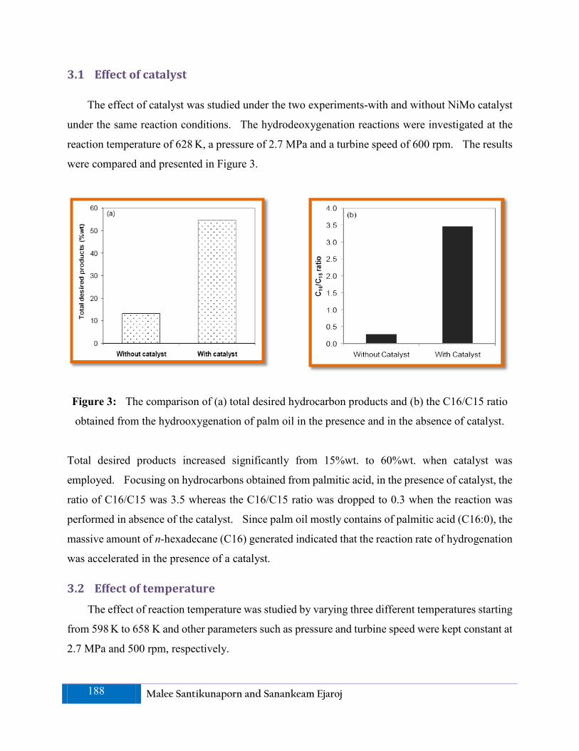
3.1 Effect of catalyst

The effect of catalyst was studied under the two experiments-with and without NiMo catalyst

under the same reaction conditions. The hydrodeoxygenation reactions were investigated at the

reaction temperature of 628 K, a pressure of 2.7 MPa and a turbine speed of 600 rpm. The results

were compared and presented in Figure 3.

Figure 3: The comparison of (a) total desired hydrocarbon products and (b) the C16/C15 ratio

obtained from the hydrooxygenation of palm oil in the presence and in the absence of catalyst.

Total desired products increased significantly from 15%wt. to 60%wt. when catalyst was

employed. Focusing on hydrocarbons obtained from palmitic acid, in the presence of catalyst, the

ratio of C16/C15 was 3.5 whereas the C16/C15 ratio was dropped to 0.3 when the reaction was

performed in absence of the catalyst. Since palm oil mostly contains of palmitic acid (C16:0), the

massive amount of n-hexadecane (C16) generated indicated that the reaction rate of hydrogenation

was accelerated in the presence of a catalyst.

3.2 Effect of temperature The effect of reaction temperature was studied by varying three different temperatures starting

from 598 K to 658 K and other parameters such as pressure and turbine speed were kept constant at

2.7 MPa and 500 rpm, respectively.


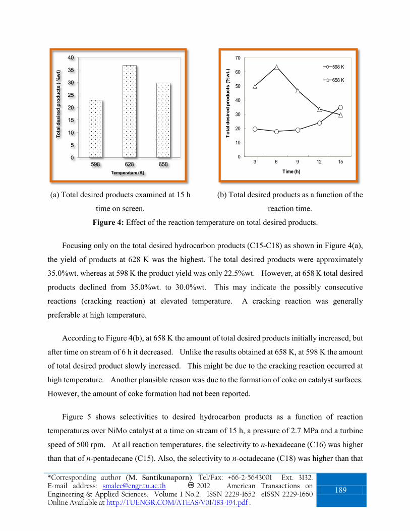
(a) Total desired products examined at 15 h

time on screen.

(b) Total desired products as a function of the

reaction time.

Figure 4: Effect of the reaction temperature on total desired products.

Focusing only on the total desired hydrocarbon products (C15-C18) as shown in Figure 4(a),

the yield of products at 628 K was the highest. The total desired products were approximately

35.0%wt. whereas at 598 K the product yield was only 22.5%wt. However, at 658 K total desired

products declined from 35.0%wt. to 30.0%wt. This may indicate the possibly consecutive

reactions (cracking reaction) at elevated temperature. A cracking reaction was generally

preferable at high temperature.

According to Figure 4(b), at 658 K the amount of total desired products initially increased, but

after time on stream of 6 h it decreased. Unlike the results obtained at 658 K, at 598 K the amount

of total desired product slowly increased. This might be due to the cracking reaction occurred at

high temperature. Another plausible reason was due to the formation of coke on catalyst surfaces.

However, the amount of coke formation had not been reported.

Figure 5 shows selectivities to desired hydrocarbon products as a function of reaction

temperatures over NiMo catalyst at a time on stream of 15 h, a pressure of 2.7 MPa and a turbine

speed of 500 rpm. At all reaction temperatures, the selectivity to n-hexadecane (C16) was higher

than that of n-pentadecane (C15). Also, the selectivity to n-octadecane (C18) was higher than that

0

5

10

15

20

25

30

35

40

598 628 658

Tota

l des

ired

prod

ucts

( %

wt)

Temperature (K)

0

10

20

30

40

50

60

70

3 6 9 12 15

Tot

al d

esir

ed p

rodu

cts

(%w

t.)

Time (h)

598 K

658 K


189



of n-heptadecane (C17). As previously reported, the C16 and C15 products were obtained from

the conversion of the palmitic acid (C16:0), but under different pathways. Generally, the C16

product was produced via the hydrogenation of palmitic acid, but the C15 product was produced

via decarbonylation and decarboxylation. Thus, it can be concluded that under these reaction

conditions the products containing the same number of carbon atoms as feed were preferred. The

explanation was also valid for the case of oleic (C18:1) and linoleic acids (C18:2). Moreover,

from Figure 6 when focused on the ratios of C16 to C15 and C18 to C17, these two ratios decreased

as the reaction temperature increased. This indicated that the decarbonylation/decarboxylation

prefers at high temperature. This might be due to the thermodynamics favor. In addition, the

cracking reaction of longer hydrocarbons was more pronounced at higher temperature.

Figure 5: Selectivity to desired products as a function of temperature.

Figure 6: The Cn+1/Cn ratio as a function of reaction temperature.

0.00.51.01.52.02.53.03.54.04.55.0

580 600 620 640 660 680

C n+1

/Cn

ratio

Temperature (K)

C16/C15C18/C17


3.3 Effect of Turbine Speed The reaction of palm oil over NiMo/Al2O3 at two different turbine speeds was compared.

Samples were collected at time on stream of 24 and 45 h. The results are presented in Figure 7(a),

7(b) and 7(c). It was obviously seen that total desired products increased when the reaction was

performed at a turbine speed of 600 rpm. It can therefore be speculated that at higher turbine

speed more desired products was likely to be generated perhaps due to the elimination of

mass-transfer limitation. However, more products especially <C14 products was observed when

collected sample at longer time (45 h). This situation should be occurred if the consecutive

reactions existed. Concentrated on product selectivity, it can be concluded that the turbine speed

does not change the selectivity of products.

Figure 7: Effect of turbine speed.

0

10

20

30

40

50

60

70

80

90

500 600

Tota

l des

ired

prod

ucts

(%w

t)

Turbine Speed (rpm)

24 h 45 h(a)

0

10

20

30

40

50

60

70

24 45

Sele

ctiv

ity to

(%)

Time (h)

Other n-C15n-C16 n-C17n-C18

(b) 500 rpm

0

10

20

30

40

50

60

70

24 45

Sele

ctiv

ity to

(%)

Time (h)

Other n-C15n-C16 n-C17n-C18

(c) 600 rpm


191



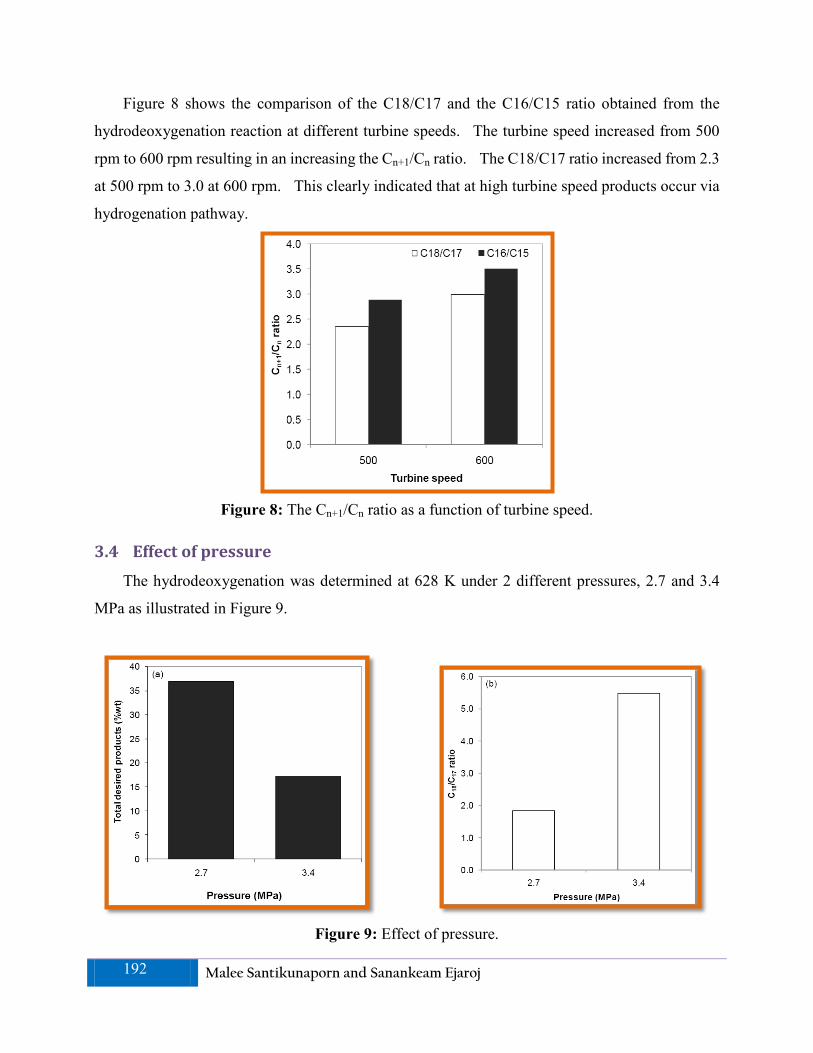
Figure 8 shows the comparison of the C18/C17 and the C16/C15 ratio obtained from the

hydrodeoxygenation reaction at different turbine speeds. The turbine speed increased from 500

rpm to 600 rpm resulting in an increasing the Cn+1/Cn ratio. The C18/C17 ratio increased from 2.3

at 500 rpm to 3.0 at 600 rpm. This clearly indicated that at high turbine speed products occur via

hydrogenation pathway.

Figure 8: The Cn+1/Cn ratio as a function of turbine speed.

3.4 Effect of pressure The hydrodeoxygenation was determined at 628 K under 2 different pressures, 2.7 and 3.4

MPa as illustrated in Figure 9.

Figure 9: Effect of pressure.


The results demonstrated that the amount of total desired products at 2.7 MPa is roughly 35.5

%wt., whereas the total desired products at 3.4 MPa drop dramatically to nearly 17 %wt. The

selectivity ratio increased dramatically from 1.83 at reaction pressure of 2.7 MPa to 5.47 when

reaction pressure was increased to 3.4 MPa. This obviously suggested that at higher reaction

pressure the hydrogenation reaction path was favored.

4. Conclusion Catalytic hydrodeoxygenation of palmitic acid was performed over NiMo catalyst in a batch

reactor. The major liquid products were pentadecane, hexadecane, heptadecane, and octadecane,

which can be categorized in a diesel range. NiMo showed a high activity for the

hydrodeoxygenation of palm oil. The yield of desired products significantly depended on the

reaction conditions. It was the highest at a moderate temperature. Further increase of pressure,

however, lower the amount of desired products. Unlike pressure, the amount of desired products

increased with the turbine speed. Finally, under the studied conditions, the Cn/Cn+1 ratios were

more than 1. This may suggested that hydrocarbon products are produced via the hydrogenation

pathway.

5. Acknowledgements PTT public company limited is gratefully acknowledged for financial support. The authors

also thank the Department of Chemical Engineering, Faculty of Engineering, Thammasat

University for providing facilities.

6. References Asavatesanupap, C. and M. Santikunaporn (2010) A Feasibility Study on Production of Solid

Fuel from Glycerol and Agricultural Wastes. International Transaction Journal of Engineering, Management, & Applied Sciences & Technologies: Vol.1: 43-51.

Bressler , D.C. and K.D. Maher. (2007) Pyrolysis of triglyceride materials for the production of renewable fuels and chemicals, Bioresource Technology, 98; pp.2351-2368.

Erhan, S.Z. , B.K. Sharma, A. Adhvaryu, and Z. Liu (2006) Chemical Modification of Vegetable Oils for Lubricant Applications. JAOCS, 83; pp.129-136.


193



Gawrilow, I. Palm Oil Usage in Lubricants (2003) 3rd Global Oils and Fats Business Forum, USA.

Lamb, H.H., J.G. Immer (2009) Catalytic Deoxygenation of Free Fatty Acids over Pd/C, North Carolina State University, Raleigh.

Lee, D.W., Y.M. Park, K.Y. Lee (2009) Heterogeneous Base Catalysts for Transesterification in Biodiesel Synthesis. Catal. Surv Asia, 13; pp.63–77.

Morgan, T., D. Grubb, E.Santillan-Jimenez, M.Crocker (2010) Conversion of Triglycerides to Hydrocarbons Over Supported Metal Catalysts, Chemistry and Materials Science. 53; pp. 820-829.

Santikunaporn, M. and S.Danphitak. (2010) Hydrodeoxygenation of Linoleic Acid on Ni-Mo Catalyst, Thammasat International Journal of Science and Technology, 15; pp.1-6.

Scrimgeour, C., (2005) Bailey’s Industrial Oil and Fat Products, F. Shahidi (Ed), Chemistry of Fatty Acids, John Wiley & Sons, Inc., Dundee, pp.1-43.

Vanichseni, T., S. Intaravichai, B. Saitthiti, and T. Kiatiwat (2002) Potential Biodiesel Production from Palm Oil for Thailand, The Kaset. Journal, 36; pp.83-97.

Vargas, R.M., U.Schuchardt, and R.Sercheli (1998) Transesterification of Vegetable Oils: a Review, J. Braz. Chem. Soc, 9; pp.199-210.

M. Santikunaporn is an Assistant Professor of Department of Chemical Engineering at Thammasat University. She earned her PhD (Chemical Engineering) from University of Oklahoma, USA. Her research work is focusing on catalytic reaction, biofuel and renewable energy.

Sanunkheam Echaroj is a master degree candidate studying Chemical Engineering at Thammasat University. He is interested in experimenting biofuel and renewable energy.






Call-for-Papers:





More Research Publication Available at

http://TUENGR.COM/ATEAS

Submit your science research today.


ATEAS V1(2):: American Transactions on Engineering & Applied Sciences

Documents

Transcript of ATEAS V1(2):: American Transactions on Engineering & Applied Sciences