At-the-time and Back-in-time Persistent SketchesBenwei Shi, Zhuoyue Zhao, Yanqing Peng, Feifei Li, Jeff M. Phillips

University of Utah

Salt Lake City, USA

benwei,zyzhao,ypeng,lifeifei,jeffp@cs.utah.edu

ABSTRACTIn the era of big data, more and more applications require the in-

formation of historical data to support rich analytics, learning, and

mining operations. In these cases, it is highly desirable to retrieve in-

formation of previous versions of data. Traditionally, multi-version

databases can be used to store all historical values of the data in or-

der to support historical queries. However, storing all the historical

data can be impractical due to its large space consumption. In this

paper, we propose the concept of at-the-time persistent (ATTP) and

back-in-time persistent (BITP) sketches, which are sketches that ap-

proximately answer queries on previous versions of data with small

space. We then provide several implementations of ATTP/BITP

sketches which are shown to be more efficient compared to existing

state-of-the-art solutions in our empirical studies.

CCS CONCEPTS• Information systems→ Data streaming; • Theory of com-putation→ Sketching and sampling.

KEYWORDSdata sketching; random sampling; persistent data structure; stream-

ing algorithms

ACM Reference Format:Benwei Shi, Zhuoyue Zhao, Yanqing Peng, Feifei Li, Jeff M. Phillips. 2021.

At-the-time and Back-in-time Persistent Sketches. In Proceedings of the2021 International Conference on Management of Data (SIGMOD ’21), June18–27, 2021, Virtual Event, China. ACM, New York, NY, USA, 14 pages.

https://doi.org/10.1145/3448016.3452802

1 INTRODUCTIONIncreasingly, in the era of big data, more applications require the

storage of and access to all historical data to support rich analytics,

learning, and mining operations. As data sources grow rapidly,

it is becoming commonplace to make snap decisions about these

data sets interactively in real time. This data is quickly classified,

or scanned for anomalies, or used to predict valuation. In each

case this data is also often used to update a model. After that, the

data may be discarded (in private messenger), passed along (on a

router, a self-driving car), or archived (at a large internet company)

but where retrieval is at a much higher cost than now. In these

scenarios the model is built and updated online, and as is crucial

Permission to make digital or hard copies of all or part of this work for personal or

classroom use is granted without fee provided that copies are not made or distributed

for profit or commercial advantage and that copies bear this notice and the full citation

on the first page. Copyrights for components of this work owned by others than the

author(s) must be honored. Abstracting with credit is permitted. To copy otherwise, or

republish, to post on servers or to redistribute to lists, requires prior specific permission

and/or a fee. Request permissions from permissions@acm.org.

SIGMOD ’21, June 18–27, 2021, Virtual Event, China© 2021 Copyright held by the owner/author(s). Publication rights licensed to ACM.

ACM ISBN 978-1-4503-8343-1/21/06. . . $15.00

https://doi.org/10.1145/3448016.3452802

0 5 10

Number of Logs (×109)

0

10

20

30

Mem

ory

Usa

ge(G

B)

SAMPLING

CMG

VERTICA

VERTICA WINDOWED AGG

0 5 10

Number of Logs (×109)

0

50

100

150

Ave

rage

quer

yti

me

(s)

SAMPLING

CMG

VERTICA

VERTICA WINDOWED AGG

Figure 1: Memory usage (left) and average query time (right)vs total number of logs inserted using ATTP sketches (SAM-PLING and CMG) and a state-of-the-art columnar store (Ver-tica), for temporal heavyhitter queries in (0, t] over 10 copiesof 98world cupwebsite access logs. VERTICA: store full datain Vertica. VERTICA_WINDOWED_AGG: store daily aggre-gated data in Vertica. The lines for SAMPLING and CMGoverlap in both figures.

for any prediction step, it evolves over time as data arrives. But

if something goes wrong in the model and we want to audit the

process, or we want to revert to an older version, or we want to

study the historical effects of the data via a summary, these tasks

are often impossible or too costly in these settings.

Our proposed solution is to build sketches which can handle

these tasks approximately, for which, under traditional models

there are large array of techniques [21, 67]. However, these are

typically designed to work over all of the data from the history

(up to now), and existing data summaries do not support tempo-

ral analytics: those queries and analytical operations that involve

filtering conditions on the temporal dimension. Thus, while these

summaries can only answer data queries and analytics about all of

the data, their efficacy demonstrates that approximation is tolerable

in many practical applications [21, 67].

An alternative solution to address these application needs are

multi-version databases or more simply to store time stamps in

an OLAP database [48, 63]. However, these solutions can be costly

when there are a large number of records accumulated over time.

In Figure 1, we compare the scalability of two of our proposed

sketches (SAMPLING and Chain Misra-Gries (CMG)) with keeping

all data, or daily aggregated data in a state-of-the-art columnar store

(Vertica), in terms of memory usage and average query time.We find

that, even with a columnar store that highly compresses the data

and leverages advanced query processing techniques such as SIMD,

storing and querying based on full data (or windowed aggregates)

becomes increasingly expensive compared to our sketches.

Another potential solutionmay be approximate query processing

(AQP) [2, 12, 21, 41, 50, 87]. It provides an appealing alternative

for big data analytics when approximations are acceptable; this is

especially useful towards building interactive analytical systems,

when exact queries become expensive over big data. But these

do not currently support temporal or persistent queries, and our

proposed sketches will complement these systems in these tasks.

Our Results. This paper proposes a framework and designs tech-

niques that extend and combine AQP with temporal big data. In

particular, instead of (or on top of) using a multi-version database,

this paper proposes the design and implementation of persistentdata summaries that offer interactive temporal analytics with strongtheoretical guarantees on their approximation quality. We will design

a series of data summarization tools which answer queries about

any point in the history of the data. These summaries do not require

significantly more space or are not significantly harder to maintain

than the summaries used for all of the data.

A natural approach to these challenges is to downsize the data by

sampling. While query sampling is a decades-old concept, and has

been explored recently in systems like BlinkDB [3], DBO [41, 41], G-

OLA [86], and XDB [51], samples do not directly offer the desired

persistence properties needed for the critical temporal analysis

tasks. Hence, it is also important to explore how to turn samples and

other data summaries (various synopses and sketches) persistent.

Specifically this paper makes the following contributions:

• We introduce two new and useful models for temporal analytics

on a data stream which are amenable to sketching, and offer

efficient and useful queries: These are At-The-Time-Persistence

(ATTP) which allows one to query the state of data at a specific

point in the past, and Back-In-Time-Persistence (BITP) which

allows queries from a prior point in time up until now.

• We provide a variety of new sketching techniques for ATTP

and BITP that build on existing streaming sketches which have

demonstrated their immensive effectiveness in numerous previ-

ous studies. These include sampling-based sketches (weighted

and unweighted), linear sketches (e.g., count-min sketch, count

sketch), and space-efficient deterministic mergeable sketches

(e.g., Misra Gries and Frequent Directions).

• For each such sketch we provide proof of the total space and

update time. They are all independent of the stream (where prior

temporal sketches often have assumptions) and in most cases

have nearly the same bound as the standard streaming sketches.

• We conduct a thorough experimental evaluation on several large

data sets focusing on the heavy-hitters and matrix-covariance

sketching problems.We provide a fair comparison across variants,

and demonstrate numerous situations where the new sketches

provide clear and sizeable advantages over the state-of-the-art.

2 PRELIMINARIES2.1 Stream ModelsA data stream A is defined by a sequence of items with timestamps

A = ((a1, t1), (a2, t2), . . . , (an , tn )), where each ai is an object and

ti is a timestamp that ti < ti+1 (for simplicity in descriptions, we

assume there are not ties, but that is addressed in code through an

assigned canonical order). The object ai could take on several forms:

it could be an index ei from a fixed (but typically large) universe [d]

like IP addresses; it could be a vector ai ∈ Rd, representing a row

in a matrix A ∈ Rn×d ; and it could be a pair ai = (ei ,wi ) where eiis again an index, andwi is a weight of that index (which could be

negative, or a count ci , and in many cases is always 1).

2.2 Data SummariesThere are many forms of data summaries [21, 57, 67, 84]. A sketchS is a data structure representation of A, but uses space sub-linearin A, and S allows specific queries for which it has approximation

guarantees. There are several general models that most sketches

fall under, and our analysis of persistent summaries will use these

general properties, which then imply results for many specific

classes of queries. First, a random sample is a powerful common

summary of A. Indeed, any robust and meaningful data analysis

which relies on the assumption thatA is i.i.d. from some distribution

will allow some sort of approximation guarantee associated with a

random sample. For some classes of queries or goals, it is useful to

allow for weighted random sampling, e.g., sampling each element

ai proportionally to an implicit or explicit weight w(ai ); theseare generally methods which reduce the variance of estimators

using importance sampling (e.g., with sensitivity sampling [34] or

leverage scores [57], for instance, used in randomized algorithms

for matrices and data).

Second, a linear sketch is (an almost always random) data struc-

ture S where each data-value S[j] is a linear combination of the data

stream elements: that is for instance in the index-count pair model

where ai = (ei , ci ) then S[j] = α(e1)c1 + α(e2)c2 + . . . + α(en )cn , orin matrix sketching setting, the αs represent a fixed (but randomly

chosen) linear transformation (e.g., a JL projection). Notably, any

linear sketch can handle negative values of ci (e.g., subtractions).Third, amergeable summary [1] is a sketch S which for an approx-

imation error ε has a size sizeε (S), and given two such summaries

S1 and S2 of data sets A1 and A2 with the same size error guaran-

tee ε and sizeε (S1) = sizeε (S2), they can be used to create a single

summary S = mergeε (S1, S2) of A = A1 ∪ A2 of the same error εand size sizeε (S) without re-inspecting A1 or A2. In some cases,

the size depends (mildly) on the size of A, and the error may in-

crease by some α on each merge operation; in this case we call it an

α-mergeable sketch. Linear sketches are mergeable (since linear op-

erations are commutative under addition). Random samples can be

made mergeable if they are implemented by assigning each element

a random value, and then maintaining the top k of these values in

a priority queue; although these samples are without replacement

and much analysis uses with-replacement samples, it can be made

with-replacement by a careful secondary subsample at the time

of analysis. Moreover, a without-replacement sample has negative

dependence which has as good and typically better convergence

properties than fully-independent ones. However, other types of

sketches (e.g., deterministic ones) are also known to be mergeable.

We next survey several relevant and exemplar types of sketches

and the best-known results within these general frameworks.

2.2.1 Frequency estimation and heavy hitters. Given a list A =⟨a1,a2, · · · ,an⟩, the frequency of j ∈ [d], denoted by f (j) = |i ∈[1,n] | ai = j|, is the count of j in A. An ε-approximate frequencyestimation summary (an ε-FE summary) of A, for all j, can return

ˆf (j) such that f (j) − εn ≤ ˆf (j) ≤ f (j) + εn. Various summaries

provide stronger bounds by either having no error on one of the two

inequalities, or replacing the εn termwith εnwhere n can depend onthe “tail.” Although these improvements carry throughwith our new

models, for simplicity, we mainly ignore them. An ε-approximate

heavy hitters summary ofA returns a list of indices j1, j2, . . . , for

parameter α , with any index j ∈ [d] which satisfies f (j) > αn, andno index j that has f (j) < αn − εn. An ε-FE summary is sufficient

for an ε-approximate heavy hitters summary, but depending on its

structure may require different time to retrieve the full list.

A random sample of size k = O(1

ε2 log1

δ

)provides an ε-FE

summary with probability at least 1 − δ .The popular CountMin sketch [22] is a linear sketch which

provides an ε-FE sketch with probability 1 − δ using O(1

ε log1

δ

)space. The Count sketch [11] is another linear sketches that uses

O(1

ε2 log1

δ

)space, but has a slightly stronger guarantee so the

εn is replaced with ε√∑d

j=1 f (j)2, which is much smaller than εn

when the distribution is skewed.

The Misra-Gries [61] and SpaceSaving sketches [60] are deter-

ministic sketches that provide ε-FE summaries; they are mergeable

and isomorphic to each other [1], and require O(1/ε) space.

2.2.2 Matrix estimation. There are many sketches for matrix es-

timation [57, 84], and its many applications in data mining and

machine learning. We focus on the setting where rows of an n × d

matrix A appear one-by-one, and the ith row ai ∈ Rd, is a d-

dimensional vector. Our desired sketch, which we call an ε-matrixcovariance sketch (or ε-MC sketch) will be an ℓ × d matrix B (or

will be able to reconstitute such a matrix), which will guarantee

that ∥ATA − BT B∥2 ≤ ε ∥A∥2F . This for instance ensures for any

unit vector x ∈ Rd that ∥Ax ∥ − ∥Bx ∥2 ≤ ε ∥A∥2F , and by increasing

the size ℓ by any additive factor k < ℓ that the covariance error isat most ε ∥A −Ak ∥

2

F /∥A∥2

F , or by increasing the size ℓ by a multi-

plicative factor k that ∥A − πBk (A)∥2

F ≤ ε ∥A − Ak ∥2

F where Ak is

the best rank-k approximation of A, and πH is a projection oper-

ator onto the subspace spanned by H [36]. While there are other

sorts of matrix approximation bounds [57, 84], ones which are not

directly related to this one, many different sketching algorithms

satisfy these bounds, and it is directly computable in empirical

evaluation [26].

Aweighted random sampling, weighted asw(ai ) = ∥a∥2, achieves

this bound with ℓ = O(d/ε2) rows [4, 26]. Linear sketches also can

achieve this error using ℓ = O(d/ε2) when based on JL random

projections [69] or more efficiently for sparse data based on the

Count sketch using ℓ = O(d2/ε2) [14, 62]; both of these bounds

can actually be tightened significantly when the numeric rank is

large, for instance when ∥A∥2F /∥A∥2

2= Ω(1/ε), then we only need

ℓ = O(1/ε) [18]. And deterministic mergeable sketches based on

Frequent Directions (an extension of the Misra-Gries [61] frequent

items sketch) attains this error using ℓ = O(1/ε) [36].Other approaches, like leverage score sampling [30], can provide

stronger relative error bounds as well, but are more challenging

to generate efficient streaming sketches [29]. One approach [17]

maintains a sample of rows B, and uses this to estimate the (ridge)

leverage score of each incoming row, and then retains it propor-

tional to this value. It never discards any sampled data, and provides

a (α , ε)-MC sketch B which ensures with constant probability that

(1 − α)ATA − εI ≺ BT B ≺ (1 + α)ATA + εI ,

that is, almost (1 ± α)-relative error in all directions, and using

O(1

α 2d logd log

(α ∥A∥2

2/ε) )

rows.

2.2.3 Quantiles estimation. In this setting, each ai in the stream is

a real value in R; in fact, any family of objects with a total order and

a constant time comparison operator can be the input. For a value

τ ∈ R, let Aτ = |a ∈ A | a ≤ τ |/|A| be the fraction of items in the

stream at most τ . An ε-quantile summary should be able to answer

either of the following queries for all instances of the query:

(1) given a value τ ∈ R report Aτ , an estimate of Aτ so that

|Aτ −Aτ | ≤ ε .(2) given a threshold ϕ ∈ (0, 1] report a value τ so |Aτ −ϕ | ≤ ε .

A random sample of size k = O(1

ε2 log1

δ

)is again an ε-quantile

summary with probability 1 − δ . A long series of work has culmi-

nated in a ε-quantiles sketch of size k = O(1

ε log log1

εδ

)[46], and

the size increases slightly to k = O(1

ε log2log

1

εδ

)if it is merge-

able [46]; these constructions hold with probability 1 − δ .

2.2.4 Approximate Range Counting Queries and KDEs. The quan-tiles query can be seen to approximate a 1-dimensional distribution.

To generalize it to higher dimensions one needs to specify a method

to query the data – a range counting query. Here we letA ⊂ Rd , andconsider a family of ranges R. An range r ∈ R returns the number

of points in that range r (A) = |a ∈ A | a ∈ r |. A useful combina-

torial measure of this is the VC-dimension [79] ν ; for axis-alignedrectangles ν = 2d , for disks ν = d + 1, for halfspaces ν = d . Thenan ε-approximate range counting (ε-ARC) summary S satisfies that

maxr ∈A

r (A)|A | −

r (S )size(S )

≤ ε . The ε-ARC summaries are typically

subsamples so size(S) = |S | is just the number of points in S .

A random sample of size k = O(1

ε2 (ν + log1

δ ))is an ε-ARC sum-

mary with probability 1 − δ [52]. Smaller summaries exist [13, 83],

including mergeable ones [1] of size k = O((1/ε)

2νν+1 log

2ν+1ν+1 1

εδ

);

for the special case of axis-aligned rectangles this can be reduced

to O((1/ε) log2d+3/2 1

εδ

). These succeed with probability ≥ 1 − δ .

Another interpretation of this problem is to allow queries with

kernels K (e.g., Gaussian kernels K(x ,a) = exp(−∥x − a∥2)). Thenan ε-KDE coreset S preserves the worst case error on a kernel

density estimate kdeA(x) = 1

|A |∑a∈A K(x ,a); that is ∥kdeA −

kdeS ∥∞ = maxx ∈Rd |kdeA(x) − kdeS (x)| ≤ ε . A random sample of

size k = O(1

ε2 log1

δ

)achieves this for any positive definite kernel,

regardless of the dimension [56, 75]. For dimensions d < 1/ε2, this

can be improved to k = O(√dε ) [47, 75]; and can use the same-

weight-merge framework [1] to become mergeable using space

O(√

dε log

2 1

εδ

), with probability 1 − δ .

2.2.5 Other coresets and sketches. There are numerous other vari-

ety of coresets and sketches, including for k-means [16, 34, 35, 49,

58], and other clustering variants [37, 38]; distinct elements [7, 45],

graphs [33], optimization, and other more obscure ones. While

many of these use uniform or weighted (sensitivity-based) sam-

pling, or are linear or mergeable, we do not provide the full list.

2.3 ATTP and BITP: Problem DefinitionIn this paper, we introduce two models for persistent sketches, at-the-time persistence (ATTP) and back-in-time persistence (BITP),

which are useful in practice and allows for considerably more effi-

cient sketches. We define ATTP and BITP sketches as extensions

of traditional sketches that answer queries at any historical times-

tamps of a stream. Our main results are previewed in Table 1.

Given a stream A and two time values s < t , define As,t as thecontent of the stream which arrived in the time interval [s, t]. Lett0 be a time point before any points in the stream arrived, and tnowthe current time. Then we also define specific stream subsets as

At = At0,t and A−t = At,tnow . Our goal in this paper is to provide

summaries (e.g., coresets and sketches) of At , and A−t which we

denote as St , and S−t , respectively.While most streaming algorithms focus on summarizing the

contents At0,tnow , there have been a few works exploring time-

restricted summaries which can allow query summaries of the form

Ss,t ; which we call a for-all-times persistent (FATP) sketch. Ourfocus is however largely of the more restrictive forms St and S−t ;which we call ATTP and BITP queries respectively. While these are

indeed more restrictive, they are quite relevant corresponding to

the state of the summary (and hence data analysis context) at that

time t and queries back to some recent (a dynamically adjustable

sliding window query). Moreover, they admit, in our opinion, very

simple and elegant algorithms, small space, and fast update time.

One previous work is on the persistent Count-Min sketch (PCM)

which is FATP sketch for the ε-FE problem [82]. Its analysis heavily

relies on a “random stream model" assumption that the elements

arrive from a fixed random distribution. Their theoretical results are

not directly comparable to ours, which like most streaming space

analysis do not rely on this. FATP sketches which use sublinear

space are not possible without this assumption. The main idea is to

build piecewise-linear approximations for the counters in a Count-

Min sketch. Since the elements arrive from a fixed distribution, the

growth of these counters are linear in expectation. It can answer

FATP queries similar to a CM sketch, except it returns the median of

the counter values instead of the minimum value. To guarantee an

ε-FE FATP sketch (under the random stream model), it can handle

one-element queries usingO(1/ε2) expected space, and requires an

additional logn to handle heavy hitter queries.

The only other previous work we know of in either of these

frameworks is an ATTP model focusing entirely on the quantiles

summary [77]. This work only considers the case with additions and

deletions of data – these deletions cause numerous complications,

including a lower bound including the harmonic sequence of sketch

sizes. In contrast, our approaches mainly focus on insertion-only

streams (as is the case with most large data, e.g., routers, website

monitoring, log structures) where if there are a small number of

corrections they can be handled in a separate structure post-hoc.

This allows our algorithms to be significantly simpler and more

general (handling any summaries based on random samples [32, 81],

linear sketches [11, 22, 69], or mergeable summaries [1]).

Use cases for ATTP and BITP. Consider a system administrator

monitoring updates for a website, and building models and making

decisions based on real-time summaries of the data up to that point.

Later (say months later), they realize some poor decision was made,

then an ATTP sketch allows them to quickly go back and review

the state of the summaries, and analyze their potential mistakes

from what the state was at those times.

Table 1: Main bounds for ATTP sketches, marked if alsoBITP (see Cor. 3.1). Weighted (wt.) bounds with U -boundedweights and U = poly(n); matrix bounds assume 1 ≤

mini ∥ai ∥.

ATTP sketches BITP Sketch Size Thm

ε-quantiles X O(ε−2 logn

)R

3.1

wt. ε-quantiles X O(ε−2 logn

)R

3.3

ε-FE X O(ε−2 logn

)5.1

wt. ε-FE X O(ε−2 logn

)R

3.3

ε-FE O(ε−1 logn

)4.2

ε-ARC (ν = O(1)) X O(ε−2 logn

)R

3.1

wt. ε-ARC (ν = O(1)) X O(ε−2 logn

)R

3.3

ε-KDE X O(ε−2 logn

)R

3.1

ε-MC X O(dε−2 log ∥A∥F

)5.1

ε-MC O(dε−1 log ∥A∥F

)4.3

(α , ε)-MC O

(d2

α 2logd log

α ∥A ∥22

ε

)r

3.3

R: Randomized, includes log1

δ factor to ensure holds with probability at least 1 − δ .r: Randomized, with constant probability.

Sliding window analysis is essential when the most recent data

in a large data stream is most relevant towards understand recent

trends. Their weakness is that they provide a fixed length of history

they summarize. If one wants to expand the analysis from one day

to two days (or say 42.3 hours), this information is not captured.

However, with a BITP sketch, one can efficiently retrieve summaries

on data for any window length into the past.

More general FATP sketches, while able to handle As,t queries,for non-uniform data require linear space, or have much weaker ac-

curacy guarantees. See for instance Figure 1 where monthly check-

points in a state-of-the-art OLAP system has space grow linearly

with the size of the data, or Section 6.1 where our ATTP sketches

significantly outperform the FATP PCM sketch in accuracy as well

as update and query time as a function of memory usage.

3 ATTP AND BITP RANDOM SAMPLESA random sample is one of the most versatile data summaries.

Almost everything from frequency estimates to quantile estimates

[40] to kernel density estimates [43, 88] can be shown to have

a guaranteed approximation from a random sample of the data.

Therefore in this section, we propose a variant of random sample

summary which is made at-the-time persistent, and we will use it

as building blocks of other ATTP sketches.

Note that under the turnstile model (i.e. if we allow deletions),

the strongest guarantees are impossible, since we may insert many

items and then delete most of them. If the random sample was

entirely from the deleted set, we know nothing about what data

remains.

The classic method to maintain a random sample in a stream

is called reservoir sampling [81]. This maintains a set of k items

uniformly at random from a stream. On seeing the ith item in the

stream (after the first k which are kept deterministically), it decides

to keep it with probability k/i , and if it is kept, it replaces a randomitem from the reservoir of kept items. The maintained items are a

uniform random sample from the entire stream up to that point.

However, if after building it, we consider the stream up to a time

t (a query q over St ), and t is sufficiently smaller than the current

time instance i (for instance less than i/k) then we do not expect

to have a good estimate of that portion of the stream (it is likely

that the summary has no information at all!). Rather we modify the

algorithm to never delete any items from the reservoir. Instead, we

mark an item that would have been deleted at time i with this value

i . Then in the future, we can reconstruct a perfect uniform random

sample for any stream up to a time t from this data: we return all

items which are retained in the summary when they first appear,

but are not yet marked (for deletion) at time t ; these items in the

normal reservoir sampling summary would potentially have been

deleted at some point after time t . Since the probability of keeping

an item decreases inversely with the size of the stream, the total

number of items ever kept is O(k logn) for a stream of size n.

Lemma 3.1. For a stream of length n, the expected number ofitems kept in k independent persistent reservoir sampling is E(kSn ) =kHn ≤ k(1 + lnn), where Hn is the nth harmonic number. And withprobability at least 0.9, kSn ∈ k(1 + lnn) ∓O(

√k lnn).

Proof. For the ith of these k independent persistent reservoir

sampling, let Xi, j be the random variable of whether jth item is

kept, and Sk,n =∑ki=1

∑nj=1 Xi, j be the random variable of the total

number of items kept. We have probability mass function for Xi, j ,

Pi, j (x) =

1 − 1/j if x = 0,

1/j if x = 1.

The mean and variance of Xi, j is

E(Xi, j ) =0(1 − 1/j) + 1(1/j) = 1/i

Var(Xi, j ) =(0 − 1/j)2(1 − 1/j) + (1 − 1/j)2/j = 1/j − 1/j2 < 1/j

The mean and variance of Sk,n is

E(Sk,n ) =k∑i=1

n∑j=1

E(Xi, j ) = kn∑j=1

1

j= kHn ≤ k(1 + lnn)

Var(Sk,n ) =k∑i=1

n∑j=1

Var(Xi, j ) = kn∑j=1

(1

j−

1

j2

)≤ k lnn.

Using Chebyshev’s inequality,

P(|Sk,n − E[Sk,n ]| ≥ ∆) ≤ Var(Sk,n )/∆2 ≤ (k lnn)/∆2 = δ .

Solving for ∆ =√(k lnn)/δ .

In many cases, it is also useful to maintain k uniform samples

without replacement. This is simple to accomplish with a priority

queue inO(logk) worst case, andO(1) amortized time per element.

Each new element ai in a stream is assigned a uniform random

number ui ∈ [0, 1] and is kept if that number is among the top klargest numbers generated. The priority queue is kept among these

top k items, and a new item is compared to the kth largest value

(maintained separately) before touching the priority queue.

Implications. For any sketch which requires a random uniform

sample of size k , we can extend it to a streaming at-the-time persis-

tence sketch with an extra factor logn in space.

Theorem 3.1. On a stream of size n, using a persistent randomsample, ATTP summaries can solve the following challenges withprobability at least 1 − δ :

• ε-quantiles summary with O(1

ε2 lognδ

)space,

• ε-FE sketch with O(1

ε2 lognδ

)space,

• ε-ARC sketch with VC-dimension ν with O(νε2 log

nδ

)space,

• ε-KDE sketch with O(1

ε2 lognδ

)space.

3.1 Persistent Weighted Random SamplesThis can be extended to weighted reservoir sampling techniques.

Consider a set of items in a streamA = ⟨a1,a2, . . . ,an⟩ where eachhas a non-negative weightwi . LetWi =

∑ij=1wi be the total weight

up to the ith item in the stream. A single item is maintained, and

on seeing a new item ai it is put in the reservoir with probability

wi/Wi , otherwise the old item is retained. To sample k items with-

replacement, run k of these processes in parallel.

The analysis for the total number of samples of this algorithm

is slightly more complicated since it may be that the weights, for

instance, double every step (i.e.,wi+1 = 2wi for all i). In this case,

in expectation about half of all items are selected at any point, and

the size of the persistent summary is Ω(n). However, this results inan unrealistic ratio between weights of points, wherewn/w1 = 2

n.

It is thus common to assume that the weights are polynomially

bounded; that is, there exist a value U so that 1/U ≤ wi/w j ≤ Ufor all i, j. We say weights are U -bounded in such a setting. For

instance, it requires log2U bits to represent integers from 1 to U .

We assume logU ≪ n.

Lemma 3.2. For a stream of length n withU -bounded weights, theexpected number of items kept in k independent persistent weightedreservoir sampling is sk = O(k(logn + logU )). And with probabilityat least 0.9, the number is in the range sk ∈ O (k(logU + logn)) ±

O(√

k(logn + logU )).

Proof. We consider simulating this process by decomposing

each item of weightwi into at mostU distinct items with uniform

weights. This stream then has at most nU items, and by Lemma 3.1,

E[sk ] = O(k log(nU )) = O(k(logn + logU )), and similarly the devi-

ation from this expected value is bounded byO(√

k(logn + logU ))

with probability at least 0.9.

Without Replacement Sampling: It is not difficult to extend

this algorithmically to weighted without replacement sampling.

The simplest (near optimally [15]) is via priority sampling [32]. For

each item ai in the stream, generate a uniform random number

ui ∈ [0, 1], and create a priority qi = wi/ui . It then simply retains

the k largest priorities, again with a priority queue in O(logk)worst case time, and expectedO(1) time. It reweights those selected

as wi = maxwi ,q(k+1):n where q(k+1):n is the (k + 1)th largest

priority among all n items.

The update time improves from O(k) for with-replacement to

worst case O(logk), and expected case O(1) time. This improves

the concentration bounds, and often the empirical performance.

Theorem 3.2. For any stream with U -bounded weights, the ex-pected size of ATTP k-priority sampling is O

(k(logn + logU )

).

The proof is verbose and tedious, so we defer it to the full version.

We overview it here. We first show the hardest case is when streams

have non-decreasing weights, and it is sufficient to analyze the case

when they are all powers of 2. For each power of 2 we can borrow

from the proof for equal weight streams. To combine the analysis

of these different equal-weight substreams, we can argue starting

a substream with weight 2iat element s , is similar to having seen

about1

2i∑sj=1w j elements of those weights before. Adding the

contributions of each ordered substream provides our result.

Implications. For any sketch which requires a random weighted

sample of size k , we can extend it to a streaming at-the-time persis-

tence sketch with an extra factor logn in space. For instance, the

weighted version of frequency estimation, quantiles, and approxi-

mate range counting an item’s contribution is proportional to its

weight requires sampling proportional to its weight. The sample

size requirements are not more than with uniform weights, and

depending on the distribution may be improved.

Theorem 3.3. On a stream of size n, withU -bounded weights andU = poly(n), using a persistent random sample, ATTP summariescan solve the following challenges with probability at least 1 − δ :

• weighted ε-quantiles summary with O(1

ε2 lognδ

)space,

• weighted ε-FE sketch with O(1

ε2 lognδ

)space,

• weighted ε-ARC coreset for range space with VC-dimension ν with

O(νε2 log

nδ

)space, and

• ε-MC sketch using O(1

ε2 log∥A ∥2Fδ

)rows via norm sampling.

• (α , ε)-MC sketch using O(1

α 2d logd log

α ∥A ∥22

ε

)rows.

3.2 BITP Random SamplesA naive inverse of this procedure will require Ω(n) space to obtain

a BITP sketch, since every item, as it is seen, might be required for

a sample over a very short BITP time window. So we cannot simply

save forever every item used in a sketch. Instead, we will carefully

delete items once they would never be used again.

That is, to achieve all of the same space bounds as before, we

simulate the without replacement sampling algorithms, and when

an item has k items with larger weight which appear after it, it

can be deleted. The argument for the space bounds follows directly

from the ATTP analysis. A key difference in ATTP sketches is that

all but a vanishing fraction of the data points will never be part of

the sketch, and this can be detected with a single threshold check

in O(1) time. Hence the ATTP sketch has amortized O(1) updatetime. On the other hand, every item in a BITP sketch is part of some

sketch while it is among the most recent k items and continues to

be until there are k items after it with larger weights, so this same

bound is not available.

In particular, a naive implementation will require Ω(k) amortized

time to process each item over the course of the stream. For instance,

assume we initially deposit each item in a cache, which we batch

process when it gets sizeCk for some constant (e.g.,C = 4), to only

retain the top k items (excluding the most recent k items). This

can be done in amortized O(logk) time per item. Yet a constant

fraction (a 1/C fraction) of items will be retained, and of them a

constant fraction (a 1/2C fraction) of them will have no more than

k/2 items with larger weights. Then as we maintain these items

in a standard priority queue, their rank can still decrement Ω(k)times before there are k items with larger weights, and they are

discarded. So while this trick can reduce the constants, Ω(n) items

will still require Ω(k) time to process.

We describe a more computationally efficient way to maintain

the required items; it applies some batch operations, and therefore

the space increases by a constant factor. All kept items are main-

tained sorted by arrival order. Let there be m items kept at any

given time (recall,m = O(k logn) in expectation). Cache the next

m items that arrive. Now scan the 2m items in arrival order (new

to old). During the scan store/insert them in an auxiliary binary

tree sorted by value so it can handle insert and rank in O(logm)time. On processing, if the rank is more than k , then do not retain

the item (in the BITP sketch memory or tree). This reduces the

insert and rank cost to O(logk) since although there will be about

m items kept in the tree, we only need to keep the topO(k) of thembalanced. This scan process takes O(m logk) time. For each batch

of sizem, the scan takesO(m logk) expected time; hence each item

in any batch has amortized, expected O(logk) processing time.

Corollary 3.1. For any ATTP random sample sketch (for a ran-dom sample of size k), we can maintain a BITP sketch with the sameasymptotic size. The ATTP sketch has O(1) amortized update time,and the BITP one has O(logk) expected amortized update time.

Queries. On a query for the ATTP sketch, there are exactly

k items active at any given window. We can store these as in-

tervals, and use an interval tree to query them in k + logm =O(k + logk log logn) time.

To query the BITP sketch, the set of k active items are not neces-

sarily demarked for a time window, as up to half of the items may

still be stored in the cache and not yet processed on the scan. We

can first perform the compression scan at the time of the query,

and it takes O(k logn) time in the expected worst case.

4 FROM STREAMING TO ATTP SKETCHESIn this section, we describe a very general framework for ATTP

sketches, which works for known sketches that can be maintained

in an insertion-only stream, and provides additive error. For each

element ai in a streamA, associate it with a non-negative weightwi ,

which could always be 1, could be provided explicitly as (ai ,wi ), or

implicitly (e.g., aswi = ∥ai ∥2, in the case of matrix sketching where

ai ∈ Rd). Then for the stream up to item ai , denotedAi , let the total

weight at that point beWi =∑ij=1wi . It is also sometimes more

convenient to reference this weight at a time t asW (t), which is the

sum of all weights up to time t . If a sketch bounds a set of queries

up to εWi at all points ai , for some error parameter ε ∈ (0, 1), werefer to it as an additive error sketch.

Then our general framework is as follows. Run the streaming

algorithm to maintain a sketch s(1/ε) at all times. Keep track of

checkpoints c1, c2, . . . , ck at various points in the stream – these are

the only information retained in the ATTP sketch. Each checkpoint

c j corresponds with a time tj . In the simplest form, each checkpoint

c j stores the full stream sketch at time tj ; and then the total space

requirement is ks(1/ε), and what remains is to bound k , the number

of checkpoints needed.

To bound the number of checkpoints, we recordW (tj ) at themost

recent checkpoint, and use this to decide when to record new check-

points. At the current stream element ai ifWi −W (tj ) < εW (tj ) wedo not include a new checkpoint. If however,Wi −W (tj ) ≥ εW (tj )then we record a new checkpoint j + 1 at the time tj+1 of the pre-vious stream element ai−1 and using the state before processingai . Since the total weight between times tj and tj+1 is less than

εW (tj ), then the error for any property of the sketch cannot change

more than εW (tj ) ≤ εW (tj+1). If the total weight is bounded by

W and the minimum weight is at least 1, then because the gaps

geometrically progress, there can be at most k = O(1

ε logW).

Lemma 4.1. An ε-additive error sketch which requires s(1/ε) spacein an insertion only stream, can maintain a ATTP sketch with space

O(s(1/ε) · 1ε logW

).

Implications. Applying the above bound to the best known insertion-only streaming sketches achieves the following results. Unfortu-

nately, because of the1

ε logn overhead (for uniform weights so

W = n), these generally are not a theoretical space improvement

over the random sampling approaches.

Theorem 4.1. On a stream of size n, using checkpoints of thestreaming sketch, ATTP summaries can solve the following challengeswith probability at least 1 − δ :

• ε-quantiles summary with O(1

ε2 log log1

εδ logn)space,

• ε-FE sketch with O(1

ε2 logn)space,

• ε-ARC sketch with VC-dimension ν using

O(ε−

3ν+1ν+1 log

2ν+1ν+1 1

εδ logn)space,

• ε-KDE sketch with k = O(√

dε2 log

2 1

εδ logn)space,

• ε-MC sketch using O(1

ε2 log ∥A∥2

)rows via Frequent Directions,

assuming the 1 ≤ mini ∥ai ∥, and

• (α , ε)-MC sketch using O(d2

α 2ε log ∥A∥2

)rows via count sketch,

assuming the 1 ≤ mini ∥ai ∥.

4.1 Elementwise Improvements : Main IdeaWhen the sketch maintains a set of specific counters which have

consistent meaning during the course of the stream, then another

optimization can be performed. For instance, this property holds

for any linear sketch, but also for other ones including Misra-Gries.

We say a sketch is a h-component additive error sketch if it has this

property, and each stream element ai affects at most h components.

Then we can maintain a separate checkpoint for each counter j.If this occurred at time t then the checkpoint is labeled c j (t), and theoverall weight at this time is stillW (t). Then we only update this

checkpoint if |c j (t)−c j (tnow)| > εW (tnow). This requires extra over-head to maintain, but the advantage arises when an update affects

a constant number of counters (e.g., h = 1 for MG, h = log(1/δ ) forCMS and CS) or the total change is all weights of counters from ele-

ment ai isO(wi ). Then total number of checkpoints is still bounded

by k = O( 1ε logW ), but each checkpoint only affects one counter.

Lemma 4.2. Anh-component ε-additive error sketch in an insertiononly stream, can maintain a ATTP sketch with space O(h · 1ε logW ).

Implications. This improvement has two direct implications im-

proving both frequent items and matrix covariance sketches, mak-

ing these problems near-optimal with this improvement.

Theorem 4.2. On a stream of size n, using checkpoints of thestreaming sketch, ATTP summaries can solve the following challengeswith probability at least 1 − δ :

• ε-FE sketch with O(1

ε logn)space, and

• (α , ε)-MC sketch using O(d2

α 2ε log ∥A∥2

)rows via count sketch,

assuming the 1 ≤ mini ∥ai ∥.

4.2 Frequent Directions ImprovementThe Frequent Directions sketch is not a h-component additive error

sketch, since each (batch) update performs a SVD on the sketch,

and updates all of the values jointly. However, we can still achieve

a similar space improvement with more care.

We maintain a sketch that has full checkpoints (each a ℓ × dmatrix) and partial checkpoints (each is one d-dimensional row

vector). On a query, we find the nearest full update prior to the

query, and process the partial updates since then.

To understand how the ATTP sketch works, we first ignore the

streaming memory constraint. That is we assume (here assuming

d < n) that a d × d matrix fits in memory. We can then maintain

the covariance exactly by caching C⊤i Ci = C⊤i−1Ci−1 + aia⊤i . We

will instead use this as the basis for a residual sketch of parts not

stored since the most recent checkpoint. We can calculate the first

eigenvector v and eigenvalue σ 2ofC⊤i Ci . Using a parameter ℓ > 0,

if σ 2 > ∥Ai ∥2

F /ℓ, we make a partial checkpoint with vector σv ,

and remove this part from the caching summary C⊤i Ci ← C⊤i Ci −

σ 2vv⊤. After every ℓ partial checkpoints, wemake a full checkpoint.

The full checkpoint merges the last full checkpoint with all of the

partial checkpoints since the last full checkpoint.

It turns out that based on the mergeability of FD, to maintain

ε ∥A∥2F error, only an FD sketch of the residual C of size ℓ = 2/εis needed, and the combination of the three parts can use the FD

compression sketch B down to ℓ = 2/ε rows also. This means that

the residual covariance can be maintained as an FD sketch C of

the residual, and only requires O(ℓd) space, and the top eigenvalue

times the top eigenvector of C⊤C is stored as c1, the first row of

C after each FD update. This is detailed in Algorithm 1, where

FDℓ(C,ai ) does an update to C with row ai using a size ℓd sketch.

Why this approach is correct. We omit the time subscript i inthe rest of this section. Let matrix B stack all the partial checkpoints

at the time t ≤ i as its rows; we have B⊤B+C⊤C = A⊤A. The aboveapproach is running FD with size parameter ℓ = 2/ε on rows of

B, resulting in a summary B. By the FD bound and properties of

residual C we have ∥B⊤B − B⊤B∥2 ≤ε2∥B∥2F ≤

ε2∥A∥2F , thus

∥A⊤A − B⊤B∥2 ≤ ∥B⊤B − B⊤B∥2 + ∥C

⊤C∥2 ≤ ε ∥A∥2F .

To query the FD ATTP sketch at time t , we use the latest fullcheckpoint B which occurred before t , and then stack all of the

partial checkpoints c j which occurred before t , but after B. Thiswill represent a matrix G, and we use G⊤G to approximate A⊤A.

Theorem 4.3. The checkpoints made by Algorithm 1 with ℓ = 2/ε

form an ATTP ε-MC sketch using space O((d/ε) log ∥A ∥F∥a1 ∥).

Algorithm 1: FD ATTP Sketch

input :A = a1,a2, · · · ,aN , ℓ > 0

1 C ← 0; B ← 0; ∥A∥2F ← 0; p ← 0

2 for i := 1 to n do3 ∥A∥2F ← ∥A∥

2

F + ∥ai ∥2

4 C ← FDℓ(C,ai )

5 while ∥c1∥2 ≥ ∥A∥2F /ℓ do6 Make partial checkpoint c1 as bp+1 with timestamp i

7 Remove first row c1 from C (c2 becomes c1)

8 p ← p + 1

9 if p = ℓ then10 Make full checkpoint FDℓ(B,b1, · · · ,bℓ) as B with

timestamp i

11 p ← 0

Proof. At any query timestamp t , let A be the full stack of all

rows, and let B be the row stack of all partial checkpoints before

or at t . Let B be the stack of the last full checkpoint before or at tand the partial checkpoint which came afterwards. Let C be the FD

sketch of the residual matrix C .

∥A⊤A − B⊤B∥2 = ∥B⊤B − B⊤B +C⊤C − C⊤C + C⊤C∥2

≤ ∥B⊤B − B⊤B∥2 + ∥C⊤C − C⊤C∥2 + ∥C

⊤C∥2

≤ ε ∥B∥2F + ε ∥C ∥2

F + ε ∥A∥2

F = 2ε ∥A∥2F

The last equality holds because of B⊤B +C⊤C = A⊤A,

∥B∥2F + ∥C∥2

F = Tr(B⊤B) + Tr(C⊤C)

=Tr(B⊤B +C⊤C) = Tr(A⊤A) = ∥A∥2F .

To bound the number of partial checkpoints, we first have the

sum of all checkpoints squared norm

∑j ∥bj ∥

2 = ∥B∥2F ≤ ∥A∥2

F . In

the worst case, a checkpoint at time tj has squared norm ∥bj ∥2 =

ε ∥A(tj )∥2

F = ∥A(tj )∥2

F − ∥A(tj−1)∥2

F . The 1st checkpoint b1 is for the

first non-zero vector, say a1, since ∥a1∥2 > ε ∥a1∥

2 = ε ∥A(1)∥2F for

any ε < 1. The 2nd checkpoint b2 at time t2 > 1 has squared norm

at least ε ∥A(t2)∥2, so ∥A(t2)∥

2 ≥ ∥b1∥2+∥b2∥

2 ≥ ∥a1∥2+ε ∥A(t2)∥

2,

which means ∥A(t2)∥2 ≥

∥a1 ∥21−ε . The kth checkpoint bk at time tk ,

we have ∥A(tk )∥2

F ≥∥a1 ∥2(1−ε )k−1

. Setting ∥A∥2F = ∥A(tk )∥2

F and solving

for k ≤ 1 + log1/(1−ε )(∥A∥

2

F /∥a1∥2) = O((1/ε) log(∥A∥F /∥a1∥)),

and the total sketch size is then O(dk) as claimed.

In this algorithm description and analysis, we use the slow ver-

sion of the FD algorithm that only uses ℓ rows. In practice, we

would like to use the Fast FD algorithm [36] which uses 2ℓ rows

and batches the computation of the internal SVD, and amortizes

its cost. However, this results in an additional challenge in that the

first eigenvalue of C⊤i Ci is not always stored in the first row Ci eachstep, only once every ℓ steps. Efforts for heuristic improvements

towards the faster FD algorithm were ineffective in practice.

5 MERGEABILITY TO BITP SKETCHESFor coresets beyond linear sketches and random samples, the most

common and generic approach is called merge-reduce. Such algo-

rithms have been developed specifically, for instance, for density-

based coresets [13, 66], clustering and PCA sketches [35], and geo-

metric ones [1, 9]. The idea is to conceptually decompose the stream

into dyadic intervals based on the time items arrive. For each such

base interval (at the lowest level of the dyadic tree considered),

create a sketch. Then for each node in the dyadic interval tree,

compute a sketch by merging the two sketches which are in the

child nodes, then reduce the size so the space at each node is the

same. Reducing the size typically increases the error in an additive

fashion (so at most O(ε · logn) error at the root); for mergeable

summaries [1] the error does not increase in the reduce step. In

a streaming algorithm, we only precompute merges on same-size

summaries, and thus only maintain at most one summary of each

size, so at most logn in total.

For an ATTP sketch, we also need to ensure we can answer any

historical query, and so it is required to maintain the left edge of

the tree (any potential root, not just the current root). However, if

we ask a query that does not correspond with a single complete

subtree, we need to reconstruct the result from up to logn disjoint

subtrees; which can be reduced to log1

ε subtrees for ε-additiveerror sketches. This means we need to maintain every node within

a depth of log1

ε of a node on the left spine of the merge tree. There

are in total (logn) · 2log 1/ε = 1

ε logn such nodes.

Lets examine this another way, to understand that we can ignore

(and thus discard) summaries that are not within a depth of log1

εof the left spine, or equivalently, do occur after 2

jobjects in the

stream and account for fewer than (ε/2)2j objects in the stream. If

(a) all summaries used on a query of size at least 2jhave at most

(ε/2)2j error, and (b) including or omitting this particular summary

of representing (ε/2)2j objects (because it is on the boundary of

a query) also incurs at most (ε/2)2j error; then the total error is

at most ε2j . This argument describes why we only need nodes in

the merge tree at depth at most log 1/ε from the left spine for the

ATTP sketch.

What is useful about this above representation is that it can be

applied to a BITP sketch. Now instead of maintaining more items

near the start of the stream (on the left side of the tree), we maintain

more at the current part of the stream (on the right side of the tree).

Instead of discarding a summary containing (ε/2)2j−1 objects eachif 2

jobjects came before it, we discard it if 2

jobjects come after it.

And this can be done dynamically even if the right side of the tree

is not complete. Thus, the same size bound applies, but it results in

a BITP sketch.

Theorem 5.1. On a stream of size n, using a merge tree for anε-additive error problem that has a mergeable sketch of size s(1/ε) canproduce a ATTP or BITP sketch of sizeO(s(1/ε) 1ε logn). In particular,BITP summaries can solve the following challenges:• ε-FE sketch (using an MG sketch) with size O( 1ε2 logn), and• ε-MC sketch (using an FD sketch) with O( 1ε2 log ∥A∥

2

F ) rows, as-suming the 1 ≤ mini ∥ai ∥.Unfortunately, compared to the ATTP chaining sketches in Sec-

tion 4, this approach has two drawbacks. First, it cannot leverage

the compression for h-component ε-additive sketches (and similar

ideas applied to FD). This requires an extra factor of 1/ε in space.

Second, this approach has the additional overhead of keeping track

of when a summary can be discarded; for the chaining approach

in Section 4, this is decided as soon as it is created. But for BITP,

a separate priority queue (or similar) is required, and this adds

0 200 400

Memory Usage (MB)

0.00

0.25

0.50

0.75

1.00

Pre

cisi

on

SAMPLING

CMG

PCM HH

0 200 400

Memory Usage (MB)

0.00

0.25

0.50

0.75

1.00

Rec

all

SAMPLING

CMG

PCM HH

Figure 2: ATTP heavy hitter average precision and recallagainst total memory usage on Client-ID dataset.

additional overhead. However, it leads to a general strategy from

any mergeable sketch to a BITP sketch.

6 EXPERIMENTSWe conducted an experimental study on a real-world dataset and

a synthetic dataset to evaluate the memory consumption, perfor-

mance and scalability of the proposed ATTP and BITP sketches for

the heavy hitter and the matrix sketch applications. All experiments

were implemented as single-threaded C++ programs. While they

were run on two different processors (Intel Core i7-3820 3.6GHz

and Intel Xeon E5-1650 v3 3.50GHz), we ensured that the time

measurements in the same set of experiments were collected from

the runs on the same type of processor. For the matrix sketches,

we used the reference implementation of the LAPACK and BLAS

routines for linear algebra operators.

6.1 ATTP Heavy HittersData sets. For the ATTP heavy hitter problem, we use the 1998

World Cup website access log [5], which includes about 1.35 billion

log entries. Each log entry contains a timestamp, a client ID, and

an object ID. The client ID is the anonymized source IP address,

and the object ID is the anonymized URL in an HTTP request.

The ID numbers are assigned in a consecutive range of integers

starting from 0. There are about 2.77M distinct clients and 90Kdistinct objects, and they are stored as 32-bit unsigned integers in

our system. The timestamps are the standard UNIX timestamps,

which are stored as 64-bit unsigned integers. We treat Client-ID

and Object-ID as two datasets and run two experiments on them.

We note that Client-ID is a quite uniform dataset while Object-ID

is slightly more skewed. The highest frequency in the Client-ID

is about 3, 700 times of the average while it is 11, 800 times of the

average in the Object-ID dataset. We set the threshold for the heavy

hitters as 0.0002 and 0.01 respectively for the client ID dataset and

the object ID dataset, such that the returned heavy hitters represent

about 0.001% to 0.01% of the total number of distinct IDs in both

datasets. For each dataset and each sketch, we issue five queries in

20% incrementals of the data size at the end of all the updates and

report the average precisions and recalls.

Competitors and parameters. Besides the ATTP random sam-

pling without replacement (SAMPLING) proposed in Section 3 and

the ATTP Chain Misra Gries (CMG) that maintains elementwise

checkpoints as proposed in Section 4.1, we also include the persis-

tent Count-Min sketch (PCM_HH) in [82], where a dyadic range

0 500 1000

Stream Size (M)

0

100

200

Mem

ory

Usa

ge(M

B)

SAMPLING (k = 1e6)

CMG (ε = 2e-5)

PCM HH (ε = 0.1)

0 500 1000

Stream Size (M)

0

50

100

Mem

ory

Usa

ge(M

B)

SAMPLING (k = 5e4)

CMG (ε = 1e-3)

PCM HH (ε = 0.04)

Figure 3: ATTP heavy hitter memory usage against streamsize on Client-ID (left) and Object-ID (right) datasets.

101 102

Memory Usage (MB)

102

103

Up

date

Tim

e(s

)

SAMPLING

CMG

PCM HH

101 102

Memory Usage (MB)

10−1

100

Que

ryT

ime

(s)

SAMPLING

CMG

PCM HH

Figure 4: ATTPheavyhitter running time against totalmem-ory usage on Client-ID dataset.

100 101 102

Memory Usage (MB)

0.00

0.25

0.50

0.75

1.00

Pre

cisi

on

SAMPLING

CMG

PCM HH

100 101 102

Memory Usage (MB)

0.00

0.25

0.50

0.75

1.00

Rec

all

SAMPLING

CMG

PCM HH

Figure 5: ATTP heavy hitter average precision and recallagainst total memory usage on Object-ID dataset.

sum technique is required to efficiently query heavy hitters. We

set the universe size to be the range of the ID numbers and thus

we need to build 22 and 17 levels of persistent Count-Min sketches

for the Client-ID and Object-ID datasets respectively. We set the

parameters so that their memory usages are comparable if possible

but there are some cases where it is infeasible because of either

the restrictions on the range of the parameters or intractable run-

ning times. More specifically, we set ε = 2, 1, 0.8, 0.6, 0.4, 0.2, 0.1

(×10−4) for CMG, the sample size k = 1, 5, 10, 20, 50, 100 (×104) for

SAMPLING, and ε = 0.1, 0.08, 0.06, 0.04, 0.02, 0.01, 0.008, 0.005 for

PCM_HH, on the Client-ID dataset. On the Object-ID dataset, we

set ε = 1, 0.8, 0.6, 0.4, 0.2, 0.1 (×10−2) for CMG, the sample sizes k =1, 2.5, 5, 10, 25, 50 (×104) for SAMPLING and ε = 0.04, 0.02, 0.01,

0.007, 0.003, 0.001 for PCM_HH. In all the PCM_HH sketches in

all the following experiments, we set δ = 0.01 and ∆ = 2000 for

PCM_HH, because further decreasing δ and/or ∆ do not result in

significant improvements without incurring unacceptable running

time and/or memory usage. Our algorithms (CMG and SAMPLING)

do not require these extra parameters.

100 101 102

Memory Usage (MB)

102

103

Up

date

Tim

e(s

)

SAMPLING

CMG

PCM HH

100 101 102

Memory Usage (MB)

10−2

10−1

Que

ryT

ime

(s)

SAMPLING

CMG

PCM HH

Figure 6: ATTPheavyhitter running time against totalmem-ory usage on Object-ID dataset.

Results. Figure 2 shows the average precision and recall against

the total memory usage of the three sketches. Figure 3(left) show

the trend of memory usage increase when the stream size increases

for a select parameter setting of each type of sketch. Figure 4 shows

the total update time and query time against the total memory

usage. Over the more uniform Client-ID dataset, we find that CMG

generally can achieve the highest precision at the same memory

usage and is guaranteed to have a recall of 1. Meanwhile, SAM-

PLING’s precision and recall is not much lower than CMG and is

faster in updates. Query times are all sub-second for both CMG

and SAMPLING in our experiments. We find PCM_HH’s precision,

recall, memory consumption and update time are inferior to any of

the ATTP sketches we proposed in this paper. Note that our dataset

is 192 times larger than the one in [82], which may explain its poor

performance in our study, despite strong performance for theirs

on similar evaluations. As shown in Figure 3, PCM_HH’s memory

usage scales linearly to the stream size while sampling and CMG

scales logarithmically. To achieve the same level of precision and

recall when the data size increases, PCM_HH tends to consume

much more memory as well as CPU time compared to the proposed

ATTP sketches. PCM_HH’s update time is also at least an order of

magnitude slower than CMG and SAMPLING, making it unsuitable

for very large datasets.

Figure 5, 3(right), 6 show the same set of experiments on the

more skewed Object-ID dataset. The findings are similar but CMG

is more favored in this case. The reason is that CMG rarely needs

to make checkpoints once all the heavy items have sufficiently

large counts in the sketch and that happens much earlier when the

dataset is more skewed.

6.2 BITP Heavy HittersWe use the same dataset as in the ATTP heavy hitter experiments.

For BITP, we experimented with the Tree Misra Gries (TMG) in

Section 5 and the batched BITP priority sampling (SAMPLING)

proposed in Section 3.2 and their competitor is still PCM_HH. For

SAMPLING and TMG, since their memory usages are not mono-

tonic, we report the maximum memory they used as their memory

usages. The parameter settings are similar between TMG/SAM-

PLING and their ATTP counterparts but we use some lower values

for PCM_HH to showcase what results in a non-trivial precision.

On the Client-ID dataset, we set ε = 2, 1, 0.7, 0.5, 0.3, 0.1 (×10−4) forTMG, the sample size k = 1, 2.5, 5, 10, 50, 100 (×104) for SAMPLING

and ε = 0.01, 0.005, 0.002, 0.001m, 0.0006, 0.0003 for PCM_HH. On

101 102 103 104

Memory Usage (MB)

0.00

0.25

0.50

0.75

1.00

Pre

cisi

on

SAMPLING

TMG

PCM HH

101 102 103 104

Memory Usage (MB)

0.7

0.8

0.9

1.0

Rec

all

SAMPLING

TMG

PCM HH

Figure 7: BITP heavy hitter average precision and recallagainst total memory usage on the Client-ID dataset.

0 500 1000

Stream Size (M)

0

2000

4000

6000

Mem

ory

Usa

ge(M

B)

SAMPLING (k = 5e5)

TMG (ε = 2e-4)

PCM HH (ε = 3e-4)

0 500 1000

Stream Size (M)

200

400

600

Mem

ory

Usa

ge(M

B)

SAMPLING (k = 2e5)

TMG (ε = 2e-3)

PCM HH (ε = 5e-4)

Figure 8: BITP heavy hitter memory usage against streamsize on Client-ID (left) and Object-ID (right) datasets.

101 102 103 104

Memory Usage (MB)

103

104

Up

date

Tim

e(s

)

SAMPLING

TMG

PCM HH

101 102 103 104

Memory Usage (MB)

100

101

102

Que

ryT

ime

(s)

SAMPLING

TMG

PCM HH

Figure 9: BITP heavy hitter running time against total mem-ory usage on Client-ID dataset.

101 102 103

Memory Usage (MB)

0.00

0.25

0.50

0.75

1.00

Pre

cisi

on

SAMPLING

TMG

PCM HH

101 102 103

Memory Usage (MB)

0.85

0.90

0.95

1.00

Rec

all

SAMPLING

TMG

PCM HH

Figure 10: BITP heavy hitter average precision and recallagainst total memory usage on the Object-ID dataset.

the Object-ID dataset, we set ε = 1, 0.8, 0.6, 0.4, 0.2, 0.1, 0.08, 0.04,

0.02 (×10−2) for TMG, the sample size k = 1, 2.4, 5, 7.5, 10, 25, 50,

75, 100 (×104) for SAMPLING and ε = 0.1, 0.07, 0.03, 0.01, 0.001,

0.0005 for PCM_HH.

Figures 7, 8(left), 9 show the same set of experiments as in

the ATTP heavy hitters on the Client-ID dataset. We find that

SAMPLING-BITP works the best in the sense that it can achieve

101 102 103

Memory Usage (MB)

102

103

104

Up

date

Tim

e(s

)

SAMPLING

TMG

PCM HH

101 102 103

Memory Usage (MB)

10−2

10−1

100

101

Que

ryT

ime

(s)

SAMPLING

TMG

PCM HH

Figure 11: BITP heavy hitter running time against totalmemory usage on Object-ID dataset.

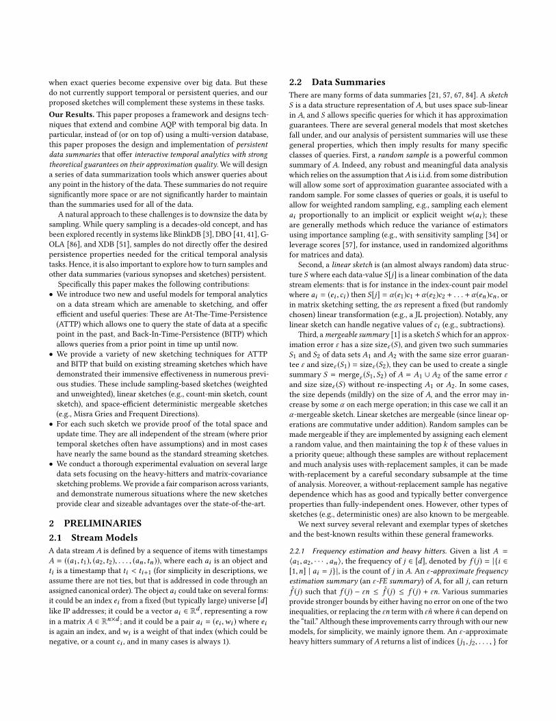
80% precision and recall using merely a reasonably small memory of

67MB. TMG, on the other hand, requires at least 14 GB of memory

to achieve a precision of 80%. Note that it only takes 18.26 GB to

store the entire log in memory. Hence, it is better off to either use

SAMPLING to save space or just store the entire data to ensure

high precision and recall on a uniform dataset. This is expected

because TMG has to maintain separate MG sketches instead of

making elementwise checkpoints in CMG, which accounts for an

additional O(1/ε) factor in space. The scalability, update and query

time are similar for both sketches. The only advantage of TMG

in this case is its guarantee of no false negative. Comparing them

to the baseline PCM_HH, we find that PCM_HH often has a poor

precision which never exceeded 50% in our experiments. While we

can expect a higher precision for PCM_HH if we set ε to be even

lower, that can result in a significantly higher update latency as

its slope of increase in update time is much steeper than TMG and

SAMPLING.

On the more skewed Object-ID dataset, the findings are similar

but the memory usage of TMG is now comparable to the other

two, thanks to the higher ε it can set to. Hence, it actually makes

sense to use TMG on a skewed dataset if we want to save space

and ensure high precision and recall at the same time. Other than

that, the trade-offs among the sketches remain the same.

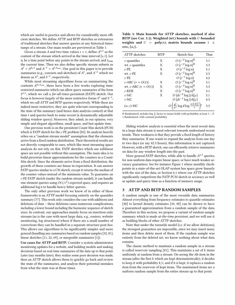
6.3 ATTP matrix estimationDatasets. For ATTP Frequent Direction, we generated three datasetswith low dimension (d = 100), medium dimension (d = 1,000) and

high dimension (d = 10,000). Each datasets contains 50,000 vec-

tors assigned to integer timestamps in [1, 1000]. Half of the vectors

are uniformly spread across all the timestamps. Each of them is

independently generated from a random orthogonal basis of Rd ,and the length of each direction follows a Gaussian distribution

with a mean of 0 and a random scale drawn from a Beta(1, 10)distribution. These vectors mimic random noises in the data. The

timestamps of the other half are distributed according to a Gaussian

distribution with a mean of 500 and a scale of 20. Each vector is

independently generated from d/10 orthogonal random directions,

and the length of each follows a Gaussian distribution with a mean

of 0 and a random scale drawn from Beta(1, 10) × 10. The secondhalf of the vectors represent special events or anomalies in the data

to be detected.

Experiment settings. For ATTP matrix estimation, there were no

established baselines in the literature to our best knowledge. Hence,

we only compare the following algorithms proposed in this pa-

per: Norm Sampling (NS) which is essentially a weighted sampling

without replacement (Section 3.1), Norm Sampling With Replace-

ment (NSWR), which is a weighted sampling with replacement

(Section 3.1), and the elementwise at-the-time-Persistent Frequent

Direction (PFD) (Section 4.2). We set ℓ = 10, 20, 40, 60, 80, 100, 150,

200 for PFD (except for the low-dimension dataset where ℓ = 150

and 200 are > d), the sample size as 10, 25, 50, 100, 150, 200, 400,

600 for NS and the same sample sizes with an additional sample

size 700 for NSWR.

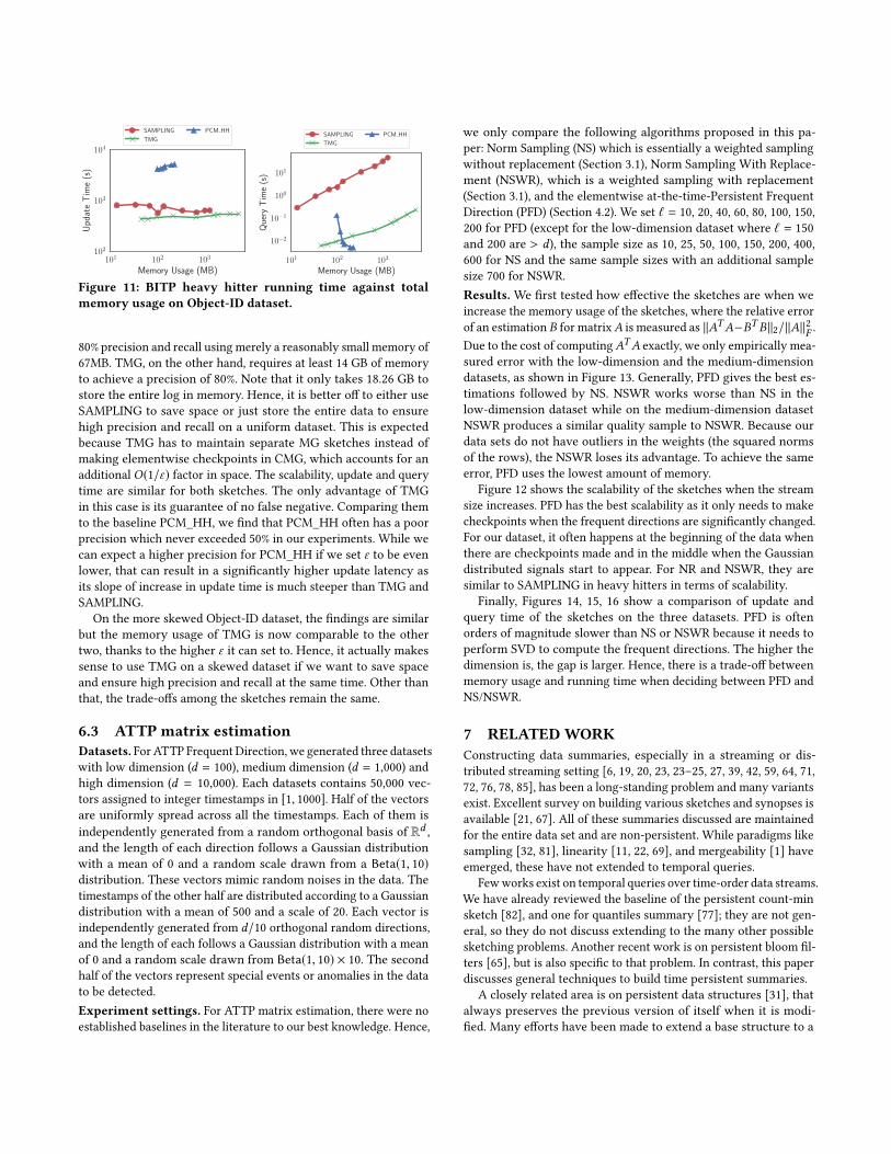
Results. We first tested how effective the sketches are when we

increase the memory usage of the sketches, where the relative error

of an estimation B for matrixA is measured as ∥ATA−BT B∥2/∥A∥2

F .

Due to the cost of computingATA exactly, we only empirically mea-

sured error with the low-dimension and the medium-dimension

datasets, as shown in Figure 13. Generally, PFD gives the best es-

timations followed by NS. NSWR works worse than NS in the

low-dimension dataset while on the medium-dimension dataset

NSWR produces a similar quality sample to NSWR. Because our

data sets do not have outliers in the weights (the squared norms

of the rows), the NSWR loses its advantage. To achieve the same

error, PFD uses the lowest amount of memory.

Figure 12 shows the scalability of the sketches when the stream

size increases. PFD has the best scalability as it only needs to make

checkpoints when the frequent directions are significantly changed.

For our dataset, it often happens at the beginning of the data when

there are checkpoints made and in the middle when the Gaussian

distributed signals start to appear. For NR and NSWR, they are

similar to SAMPLING in heavy hitters in terms of scalability.

Finally, Figures 14, 15, 16 show a comparison of update and

query time of the sketches on the three datasets. PFD is often

orders of magnitude slower than NS or NSWR because it needs to

perform SVD to compute the frequent directions. The higher the

dimension is, the gap is larger. Hence, there is a trade-off between

memory usage and running time when deciding between PFD and

NS/NSWR.

7 RELATEDWORKConstructing data summaries, especially in a streaming or dis-

tributed streaming setting [6, 19, 20, 23, 23–25, 27, 39, 42, 59, 64, 71,

72, 76, 78, 85], has been a long-standing problem and many variants

exist. Excellent survey on building various sketches and synopses is

available [21, 67]. All of these summaries discussed are maintained

for the entire data set and are non-persistent. While paradigms like

sampling [32, 81], linearity [11, 22, 69], and mergeability [1] have

emerged, these have not extended to temporal queries.

Fewworks exist on temporal queries over time-order data streams.

We have already reviewed the baseline of the persistent count-min

sketch [82], and one for quantiles summary [77]; they are not gen-

eral, so they do not discuss extending to the many other possible

sketching problems. Another recent work is on persistent bloom fil-

ters [65], but is also specific to that problem. In contrast, this paper

discusses general techniques to build time persistent summaries.

A closely related area is on persistent data structures [31], that

always preserves the previous version of itself when it is modi-

fied. Many efforts have been made to extend a base structure to a

0 20 40

Stream Size (K)

0.5

1.0

1.5

2.0

Mem

ory

Usa

ge(M

B)

NS (k = 400)

NSWR (k = 400)

PFD (` = 80)

(a) Low-dimension dataset

0 20 40

Stream Size (K)

2

4

6

8

Mem

ory

Usa

ge(M

B)

NS (k = 150)

NSWR (k = 150)

PFD (` = 150)

(b) Medium-dimension dataset

0.00 0.02 0.04

Stream Size (M)

10

15

20

25

30

Mem

ory

Usa

ge(M

B)

NS (k = 50)

NSWR (k = 50)

PFD (` = 60)

(c) High-dimension datasetFigure 12: ATTP matrix estimation memory usage against stream size.

0 1 2 3

Memory Usage (MB)

0.00

0.05

0.10

0.15

Err

or

NS

NSWR

PFD

0 10 20

Memory Usage (MB)

0.00

0.05

0.10

Err

or

NS

NSWR

PFD

Figure 13: ATTP matrix estimation relative erroragainst total memory usage on low-(left) and medium-dimension(right) data sets.

10−1 100

Memory Usage (MB)

10−2

10−1

100

101

Up

date

Tim

e(s

)

NS

NSWR

PFD

10−1 100

Memory Usage (MB)

10−3

10−2

10−1

Que

ryT

ime

(s)

NS

NSWR

PFD

Figure 14: ATTP matrix estimation running time against to-tal memory usage on the low-dimension dataset.

100 101

Memory Usage (MB)

10−1

100

101

102

103

Up

date

Tim

e(s

)

NS

NSWR

PFD

100 101

Memory Usage (MB)

10−1

100

101

Que

ryT

ime

(s)

NS

NSWR

PFD

Figure 15: ATTP matrix estimation running time against to-tal memory usage on the medium-dimension dataset.

persistent data structure, including Time-Split B-tree [55] and Mul-

tiversion B-tree [8, 10, 80]. Persistent data structures are also used

in multiversion databases such as Microsoft Immortal DB [53, 54],

SNAP [74], Ganymed [68], Skippy [73] and LIVE [70].

Another similar area is approximate query processing [2, 12, 21,

28, 41, 44, 50, 87], which also rely on sampling, and similar ideas,

including BlinkDB [3], DBO [41], G-OLA [86], Quickr [44], and

101 102

Memory Usage (MB)

100

101

102

103

104

Up

date

Tim

e(s

)

NS

NSWR

PFD

101 102

Memory Usage (MB)

101

102

103

Que

ryT

ime

(s)

NS

NSWR

PFD

Figure 16: ATTP matrix estimation running time against to-tal memory usage on the high-dimension dataset.

XDB [51]. Yet again, these store the entire data set; replacing the

internal summaries in these systems with ATTP and BITP sketches

may allow them to more easily offer temporal refinement queries

and update to new data.

8 CONCLUSIONIn this paper, we define the concept of ATTP sketches and BITP

sketches. An ATTP sketch supports queries on time ranges starting

at the beginning of history and captures the state of a streaming

summary at that time. A BITP sketch supports queries on time

ranges ending at the current timestamp, and related to a flexible

sliding window form of query. We describe the ATTP and BITP

versions of random sampling, as well as a general framework for

making sketches ATTP/BITP that build on concepts like linearity

and mergeability of sketches. In many cases, our framework allows

us to uncover sketches where space is provably almost as small

as for standard streaming algorithms. We state theoretical results

for 8 different types of sketching problems, but many more should

be direct consequences, or possible following our framework. Ex-

perimental results show that our sketches can answer ATTP/BITP

queries with low error rate in a small space, either significantly

improving on baselines or resulting in the first sketches of this type

for other scenarios.

Acknowledgments. Jeff M. Phillips thanks his support from NSF

CCF-1350888, CNS-1514520, IIS-1619287, IIS-1816149, CNS-1564287,

CFS-1953350, and an award from Visa Research. Feifei Li thanks

his support from NSF CNS-1514520, IIS-1619287, IIS-1801446, and

IIS-1816149. Zhuoyue Zhao and Yanqing Peng thank support from

Google PhD Fellowships. The authors also appreciate the valu-

able feedback from the anonymous SIGMOD reviewers in helping

improve the paper.

REFERENCES[1] P. Agarwal, G. Cormode, Z. Huang, J. Phillips, Z. Wei, and K. Yi. Mergeable

summaries. ACM Transactions on Database Systems, 38(4):1–28, 2013.[2] S. Agarwal, H. Milner, A. Kleiner, A. Talwalkar, M. I. Jordan, S. Madden, B. Moza-

fari, and I. Stoica. Knowing when you’re wrong: building fast and reliable

approximate query processing systems. In SIGMOD, 2014.[3] S. Agarwal, B. Mozafari, A. Panda, H. Milner, S. Madden, and I. Stoica. Blinkdb:

queries with bounded errors and bounded response times on very large data. In

EuroSys, 2013.[4] F. Alan, K. Ravi, and V. Santosh. Fast monte-carlo algorithms for finding low-rank

approximations. In FOCS, 1998.[5] M. Arlitt and T. Jin. A workload characterization study of the 1998 world cup

web site. Netwrk. Mag. of Global Internetwkg., 14(3):30–37, 2000.[6] B. Babcock and C. Olston. Distributed top-k monitoring. In SIGMOD, 2003.[7] Z. Bar-Yossef, T. S. Jayram, R. Kumar, D. Sivakumar, and L. Trevisan. Counting

distinct elements in a data stream. In RANDOM, pages 1–10, 2002.

[8] B. Becker, S. Gschwind, T. Ohler, B. Seeger, and P. Widmayer. An asymptotically

optimal multiversion b-tree. VLDB J., 5(4):264–275, 1996.[9] J. L. Bentley and J. B. Saxe. Decomposable searching problems I: Static-to-dynamic

transformations. Journal of Algorithms, 1(4), 1980.[10] G. S. Brodal, K. Tsakalidis, S. Sioutas, and K. Tsichlas. Fully persistent b-trees. In

SODA, pages 602–614, 2012.[11] M. Charikar, K. Chen, and M. Farach-Colton. Finding frequent items in data

streams. In ICALP, 2002.[12] S. Chaudhuri, B. Ding, and S. Kandula. Approximate query processing: No silver

bullet. In SIGMOD, pages 511–519, 2017.[13] B. Chazelle and J. Matousek. On linear-time deterministic algorithms for op-

timization problems in fixed dimensions. Journal of Algorithms, 21:579–597,1996.

[14] K. L. Clarkson and D. P. Woodruff. Low rank approximation and regression in

input sparsity time. In STOC, 2013.[15] E. Cohen, N. Duffield, H. Kaplan, C. Lund, and M. Thorup. Stream sampling for

variance-optimal estimation of subset sums. In SODA, 2009.[16] M. B. Cohen, S. Elder, C.Musco, C.Musco, andM. Persu. Dimensionality reduction

for k -means clustering and low rank approximation. In STOC, 2015.[17] M. B. Cohen, C. Musco, and J. Pachocki. Online row sampling. In APPROX/RAN-

DOM, volume 60, 2016.

[18] M. B. Cohen, J. Nelson, and D. P. Woodruff. Optimal approximate matrix product

in terms of stable rank. In ICALP, 2016.[19] G. Cormode and M. Garofalakis. Sketching streams through the net: Distributed

approximate query tracking. In Proc. International Conference on Very Large DataBases, 2005.

[20] G. Cormode, M. Garofalakis, S. Muthukrishnan, and R. Rastogi. Holistic aggre-

gates in a networked world: distributed tracking of approximate quantiles. In

SIGMOD, 2005.[21] G. Cormode, M. N. Garofalakis, P. J. Haas, and C. Jermaine. Synopses for mas-

sive data: Samples, histograms, wavelets, sketches. Foundations and Trends inDatabases, 4(1-3):1–294, 2012.

[22] G. Cormode and S. Muthukrishnan. An improved data stream summary: The

count-min sketch and its applications. Journal of Algorithms, 55:58–75, 2005.[23] G. Cormode, S. Muthukrishnan, and K. Yi. Algorithms for distributed functional

monitoring. In SODA, 2008.[24] G. Cormode, S. Muthukrishnan, and W. Zhuang. What’s different: Distributed,

continuous monitoring of duplicate-resilient aggregates on data streams. In ICDE,2006.

[25] G. Cormode, S. Muthukrishnan, and W. Zhuang. Conquering the divide: Contin-

uous clustering of distributed data streams. In Proc. IEEE International Conferenceon Data Engineering, 2007.

[26] A. Desai, M. Ghashami, and J. M. Phillips. Improved practical matrix sketch-

ing with guarantees. IEEE Transactions on Knowledge and Data Engineering,28(7):1678–1690, 2016.

[27] A. Deshpande, C. Guestrin, S. Madden, J. Hellerstein, and W. Hong. Model-driven

data acquisition in sensor networks. In VLDB, 2004.[28] B. Ding, S. Huang, S. Chaudhuri, K. Chakrabarti, and C. Wang. Sample + seek:

Approximating aggregates with distribution precision guarantee. In SIGMOD,pages 679–694, 2016.

[29] P. Drineas, M. Magdon-Ismail, M. W. Mahoney, and D. P. Woodruff. Fast approxi-

mation of matrix coherence and statistical leverage. Journal of Machine LearningResearch, 13:3441–3472, 2012.

[30] P. Drineas, M. W. Mahoney, and S. Muthukrishnan. Relative-error CUR matrix

decompositions. SIAM Journal of Matrix Analysis and Applications, 30:844–881,2008.

[31] J. R. Driscoll, N. Sarnak, D. D. Sleator, and R. E. Tarjan. Making data structures

persistent. J. Comput. Syst. Sci., 38(1):86–124, 1989.[32] N. Duffield, C. Lund, and M. Thorup. Priority sampling for estimation of arbitrary

subset sums. JACM, 54(32), 2007.

[33] J. Feigenbaum, S. Kannan, A. McGregor, S. Suri, and J. Zhang. Graph distances

in the streaming model: The value of space. In Proc. ACM-SIAM Symposium onDiscrete Algorithms, 2005.

[34] D. Feldman and M. Langberg. A unified framework for approximating and

clustering data. In Proceedings of the 43rd annual ACM symposium on Theory ofcomputing, 2011.

[35] D. Feldman, M. Schmidt, and C. Sohler. Turning big data into tiny data: Constant-

size coresets for k -means, PCA, and projective clustering. In SODA, 2013.[36] M. Ghashami, E. Liberty, J. M. Phillips, and D. P. Woodruff. Frequent direc-

tions: Simple and deterministic matrix sketching. SIAM Journal on Computing,45(5):1762–1792, 2016.

[37] S. Guha. Tight results for clustering and summarizing data streams. In ICDT,2009.

[38] S. Guha, N. Mishra, R. Motwani, and L. O’Callaghan. Clustering data streams. In

FOCS, 2000.[39] L. Huang, M. Garofalakis, A. D. Joseph, and N. Taft. Communication-efficient

tracking of distributed cumulative triggers. In ICDCS, 2007.[40] Z. Huang, L. Wang, K. Yi, and Y. Liu. Sampling based algorithms for quantile

computation in sensor networks. In Proc. ACM SIGMOD International Conferenceon Management of Data, 2011.

[41] C. Jermaine, S. Arumugam, A. Pol, and A. Dobra. Scalable approximate query

processing with the DBO engine. ACM Transactions on Database Systems, 33(4),Article 23, 2008.

[42] S. Jeyashanker, S. Kashyap, R. Rastogi, and P. Shukla. Efficient constraint moni-

toring using adaptive thresholds. In ICDE, 2008.[43] S. Joshi, R. V. Kommaraju, and J. M. Phillips. Comparing distributions and shapes

using the kernel distance. In Proceedings 27th Symposium on ComputationalGeometry, 2011.

[44] S. Kandula, A. Shanbhag, A. Vitorovic, M. Olma, R. Grandl, S. Chaudhuri, and

B. Ding. Quickr: Lazily approximating complex adhoc queries in bigdata clusters.

In SIGMOD, pages 631–646, 2016.[45] D. M. Kane, J. Nelson, and D. P. Woodruff. An optimal algorithm for the distinct

elements problem. In PODS, pages 41–52. ACM, 2010.

[46] Z. Karnin, K. Lang, and E. Liberty. Optimal quantile approximation in streams.

In Proceedings IEEE Symposium on Foundations of Computer Science, 2016.[47] Z. Karnin and E. Liberty. Discrepancy, coresets, and sketches in machine learning.

In Proceedings of the Thirty-Second Conference on Learning Theory, volume 99 of

PMLR, pages 1975–1993, 2019.[48] A. Lamb, M. Fuller, R. Varadarajan, N. Tran, B. Vandiver, L. Doshi, and C. Bear.

The vertica analytic database: C-store 7 years later. Proc. VLDB Endow.,5(12):1790âĂŞ1801, Aug. 2012.

[49] M. Langberg and L. J. Schulman. Universal ε -approximators for integrals. In

Proceedings ACM-SIAM Symposium on Discrete Algorithms, 2010.[50] F. Li, B. Wu, K. Yi, and Z. Zhao. Wander join: Online aggregation via random

walks. In SIGMOD, pages 615–629, 2016.[51] F. Li, B. Wu, K. Yi, and Z. Zhao. Wander join and XDB: online aggregation via

random walks. SIGMOD Record, 46(1):33–40, 2017.[52] Y. Li, P. Long, and A. Srinivasan. Improved bounds on the samples complexity of

learning. Journal of Computer and System Sciences, 62:516–527, 2001.[53] D. B. Lomet, R. S. Barga, M. F. Mokbel, G. Shegalov, R.Wang, and Y. Zhu. Immortal

DB: transaction time support for SQL server. In SIGMOD Conference, pages 939–941. ACM, 2005.

[54] D. B. Lomet and F. Li. Improving transaction-time DBMS performance and

functionality. In ICDE, pages 581–591, 2009.[55] D. B. Lomet and B. Salzberg. Access methods for multiversion data. In SIGMOD

Conference, pages 315–324. ACM Press, 1989.

[56] D. Lopez-Paz, K. Muandet, B. Schölkopf, and I. Tolstikhin. Towards a learning

theory of cause-effect inference. In International Conference on Machine Learning,pages 1452–1461, 2015.

[57] M. W. Mahoney. Randomized algorithms for matrices and data. Foundations andTrends in Machine Learning, NOW Publishers, 3(2), 2011.

[58] K. Makarychev, Y. Makarychev, and I. Razenshteyn. Performance of johnson-

lindenstrauss transform for k-means and k-medians clustering. In STOC, 2019.[59] A. Manjhi, V. Shkapenyuk, K. Dhamdhere, and C. Olston. Finding (recently)

frequent items in distributed data streams. In ICDE, 2005.[60] A. Metwally, D. Agrawal, and A. Abbadi. An integrated efficient solution for

computing frequent and top-k elements in data streams. ACM Transactions onDatabase Systems, 31(3):1095–1133, 2006.

[61] J. Misra and D. Gries. Finding repeated elements. Sc. Comp. Prog., 2:143–152,1982.

[62] J. Nelson and H. L. Nguyen. OSNAP: Faster numerical linear algebra algorithms

via sparser subspace embeddings. In Proceedings of 54th IEEE Symposium onFoundations of Computer Science, 2013.

[63] T. Neumann. Efficiently compiling efficient query plans for modern hardware.

Proc. VLDB Endow., 4(9):539âĂŞ550, June 2011.[64] C. Olston, J. Jiang, and J. Widom. Adaptive filters for continuous queries over

distributed data streams. In SIGMOD, 2003.

[65] Y. Peng, J. Guo, , W. Qian, and A. Zhou. Persistent bloom filter: Membership

testing for the entire history. In SIGMOD, 2018.[66] J. M. Phillips. Algorithms for ε -approximations of terrains. In ICALP, 2008.[67] J. M. Phillips. Coresets and sketches. In 3rd, editor, Handbook of Discrete and

Computational Geometry, chapter 48. CRC Press, 2016.

[68] C. Plattner, A. Wapf, and G. Alonso. Searching in time. In SIGMOD Conference,pages 754–756. ACM, 2006.

[69] T. Sarlos. Improved approximation algorithms for large matrices via random

projections. In Proceedings Symposium on Foundations of Computer Science, 2006.[70] A. D. Sarma, M. Theobald, and J. Widom. LIVE: A lineage-supported versioned

DBMS. In SSDBM, volume 6187 of Lecture Notes in Computer Science, pages416–433. Springer, 2010.

[71] I. Sharfman, A. Schuster, and D. Keren. A geometric approach to monitoring

threshold functions over distributed data streams. In SIGMOD, 2006.[72] I. Sharfman, A. Schuster, and D. Keren. Shape sensitive geometric monitoring.

In Proc. ACM Symposium on Principles of Database Systems, 2008.[73] R. Shaull, L. Shrira, and H. Xu. Skippy: a new snapshot indexing method for

time travel in the storage manager. In SIGMOD Conference, pages 637–648. ACM,

2008.

[74] L. Shrira and H. Xu. SNAP: efficient snapshots for back-in-time execution. In

ICDE, pages 434–445. IEEE Computer Society, 2005.

[75] W. M. Tai and J. M. Phillips. Improved coresets for kernel density estimates. In

Proceedings ACM-SIAM Sympoisum on Discrete Algorithms, 2018.[76] M. Tang, F. Li, J. M. Phillips, and J. Jestes. Efficient threshold monitoring for

distributed probabilistic data. In ICDE, 2012.[77] Y. Tao, K. Yi, C. Sheng, J. Pei, and F. Li. Logging every footstep: Quantile sum-

maries for the entire history. In Proc. ACM SIGMOD International Conference on

Management of Data, 2010.[78] S. Tarkoma, C. E. Rothenberg, and E. Lagerspetz. Theory and practice of bloom

filters for distributed systems. IEEE CST, 14(1):131–155, 2012.[79] V. Vapnik and A. Chervonenkis. On the uniform convergence of relative frequen-

cies of events to their probabilities. The. of Prob. App., 16:264–280, 1971.[80] P. J. Varman and R. M. Verma. An efficient multiversion access structure. IEEE

Trans. Knowl. Data Eng., 9(3):391–409, 1997.[81] J. S. Vitter. Random sampling with a reservoir. ACM Transactions on Mathematical

Software, 11(1):37–57, 1985.[82] Z. Wei, G. Luo, K. Yi, X. Du, and J. Wen. Persistent data sketching. In SIGMOD

Conference, pages 795–810. ACM, 2015.

[83] Z. Wei and K. Yi. The space complexity of 2-dimensional approximate range

counting. In Proceedings of the Twenty-Fourth Annual ACM-SIAM Symposium onDiscrete Algorithms, pages 252–264, 2013.

[84] D. P. Woodruff. Sketching as a tool for numerical linear algebra. Foundations andTrends in Theoretical Computer Science, 10:1–157, 2014.

[85] K. Yi and Q. Zhang. Optimal tracking of distributed heavy hitters and quantiles.

In PODS, pages 167–174, 2009.[86] K. Zeng, S. Agarwal, A. Dave, M. Armbrust, and I. Stoica. G-OLA: generalized on-

line aggregation for interactive analysis on big data. In SIGMOD, pages 913–918,2015.

[87] K. Zeng, S. Gao, B. Mozafari, and C. Zaniolo. The analytical bootstrap: a new

method for fast error estimation in approximate query processing. In SIGMOD,pages 277–288, 2014.

[88] Y. Zheng, J. Jestes, J. M. Phillips, and F. Li. Quality and efficiency for kernel

density estimates in large data. In SIGMOD, pages 433–444, 2013.