Asymptotically exponential hitting times and metastability...

E l e c t r o n ic

Jo

ur n a l

of

Pr

o b a b i l i t y

Electron. J. Probab. 20 (2015), no. 122, 1–37.ISSN: 1083-6489 DOI: 10.1214/EJP.v20-3656

Asymptotically exponential hitting times andmetastability: a pathwise approach

without reversibility

R. Fernandez* F. Manzo† F. R. Nardi‡ E. Scoppola§

Abstract

We study the hitting times of Markov processes to target set G, starting from areference configuration x0 or its basin of attraction and we discuss its relation tometastability.

Three types of results are reported: (1) A general theory is developed, based onthe path-wise approach to metastability, which is general in that it does not assumereversibility of the process, does not focus only on hitting times to rare events and doesnot assume a particular starting measure. We consider only the natural hypothesis thatthe mean hitting time to G is asymptotically longer than the mean recurrence time tothe refernce configuration x0 or G. Despite its mathematical simplicity, the approachyields precise and explicit bounds on the corrections to exponentiality. (2) We compareand relate different metastability conditions proposed in the literature. This is speciallyrelevant for evolutions of infinite-volume systems. (3) We introduce the notion of earlyasymptotic exponential behavior to control time scales asymptotically smaller thanthe mean-time scale. This control is particularly relevant for systems with unboundedstate space where nucleations leading to exit from metastability can happen anywherein the volume. We provide natural sufficient conditions on recurrence times for thisearly exponentiality to hold and show that it leads to estimations of probability densityfunctions.

Keywords: Metastability; continuous time Markov chains on discrete spaces; hitting times;asymptotic exponential behavior .AMS MSC 2010: 60J27; 60J28; 82C05.Submitted to EJP on July 10, 2014, final version accepted on October 11, 2015.

1 Introduction

Hitting times to rare sets, and related metastability issues, have been studied both inthe framework of probability theory and statistical mechanics.

A short review of first hitting results is given in sect. 1.1. As far as metastabilityresults are concerned, the story is much more involved due to the fact that metastabilitycan be defined in different ways.

*Mathematics Department, Utrecht University, P.O. Box 80010, 3508 TA Utrecht, The Netherlands†Dipartimento di Matematica, Università di Roma Tre, Largo S. Leonardo Murialdo 1, 00146 Rome, Italy‡Technische Universiteit Eindhoven, P.O. Box 513, 5600 MB Eindhoven, The Netherlands§Dipartimento di Matematica, Università di Roma Tre, Largo S. Leonardo Murialdo 1, 00146 Rome, Italy

http://ejp.ejpecp.org/

http://dx.doi.org/10.1214/EJP.v20-3656

Asymptotically exponential hitting times and metastability

The phenomenon of metastability is given by the following scenario: (i) A systemremains “trapped” for an abnormally long time in a state —the metastable phase— differ-ent from the eventual equilibrium state consistent with the thermodynamical potentials.(ii) Subsequently, the system undergoes a sudden transition from the metastable to thestable state at a random time.

The mathematical study of this phenomenon has been a standing issue since thefoundation of the field of rigorous statistical mechanics. This long history resulted in anumber of different approaches, based on non-equivalent assumptions.

The common feature of these mathematical descriptions is a stochastic frameworkinvolving a Markovian evolution and two disjoint distinguished sets of configurations,respectively representing metastable and stable states. Rigorously speaking, a statisticalmechanical “state” corresponds to a probability measure. The association to sets ofconfigurations corresponds, therefore, to identifying supports of relevant measures.This is a crucial step in which both probabilistic and physical information must beincorporated. Within such framework, the central mathematical issue is the descriptionof the first-exit trajectories leading from an initial metastable configuration to a finalstable one. The exit path can be decomposed into two parts:

• an escape path —taking the system to the boundary of the metastable set, whichcan be thought of as a saddle or a bottleneck: a set with small equilibrium measurewhich is difficult for the system to reach. —

• and a downhill path —bringing the system into the next stable state. —

Metastable behavior occurs when the time spent in downhill paths is negligible withrespect to the escape time. In such a scenario, the overall exponential character ofthe time to reach stability is, therefore, purely due to the escape part of the trajectory.This implies that the set of metastable states can be considered as a single state in thesense that the first escape turns out to be exponentially distributed as in the case ofa single state. Actually this exponential law can be considered as the main feature ofmetastability.

As noted above, the escape time from a metastable set can be determined fromthe first hitting time to the rare set of saddle configurations. This fact establishes anassociation between metastability and hitting times to rare events. Nevertheless, thephysical quantity in metastability studies is the transition time from the metastablephase to the stable one. The reduction of this issue to the study of hitting times to raresets requires a detailed investigation of the state space in order to determine the saddleset.

In metastability literature, the main used tools are renormalization [61, 62], cycledecomposition and large deviations [21, 22, 23, 20, 55, 56, 57, 47, 63] and, lately,potential theoretic techniques [9, 10, 12, 13, 5, 6]. Generally speaking, the focus is moreon the exit path and on the mean exit time, while the results on the distribution of theescape time are usually asymptotical and not quantitative as in [2].

At any rate, metastability involves a relaxation from an initial measure to a metastablestate, from which the systems undergoes a final transition into stability. To put thistwo-step process in evidence, the theory must apply to sufficiently general initial states.Furthermore, the phenomenon is particularly relevant for evolutions out of equilibrium,thus a comprehensive theory must not assume reversibility.

This paper is based on the path-wise approach to metastability developed in[20, 55,56, 57, 47]. This approach has led to a detailed description of exit paths in terms ofrelevant physical quantities, such as energy, entropy, temperature, etc. In this paper weshow how the same approach provides simple and effective estimations of the laws ofhitting times for rather general, not necessarily reversible dynamics. This makes our

EJP 20 (2015), paper 122./37

ejp.ejpecp.org




treatment applicable to many interesting models in the framework of non-equilibriumstatistical mechanics. Examples of non-reversible dynamics can be found in cases ofnon symmetric models, like TASEP (totally asymmetric simple exclusion process ) or ofparallel dynamics, like PCA (probabilistic cellular automata). As showed in [30] thesekind of dynamics can be much more efficient from an algorithmic point of view.

Moreover we can consider hitting to more general goals, not necessarily rare sets,so, in metastability language, we do not need to determine the saddle configurations inorder to prove the exponentially of the decay time since we can directly consider as goalthe stable state. This can be an important point to apply the theory in very complicatedphysical contexts where a detailed control of the state space is too difficult.

1.1 First hitting times: known results

The stochastic treatment was initially developed in the framework of reliability theory,in which the reference states are called good states and the escaped states are the badstates. The exponential character of good-to-bad transitions —well known from quitesome time— is due to the existence of two different time scales: Long times are neededto go from good to bad states, while the return to good states from anywhere —except,perhaps, the bad states— is much shorter. As a result, a system in a good state canarrive to the bad state only through a large fluctuation that takes it all the way to the badstate. Any intermediate fluctuation will be followed by an unavoidable return to the goodstates, where, by Markovianness, the process starts afresh independently of previousattempts. The escape time is formed, hence, by a large number of independent returnsto the good states followed by a final successful excursion to badness that must happenwithout hesitations, in a much shorter time. The exit time is, therefore, a geometricrandom variable with extremely small success probability; in the limit, exponentialityfollows.

A good reference to this classical account is the short book [44] which, in fact, collectsalso the main tools subsequently used in the field: reversibility, spectral decomposition,capacity, complete monotonicity. Exponentiality of hitting times to rare events is analyzed,in particular, in Chapter 8 of this book, where regenerative processes are considered.

The tools given in [44] where exploited in [17, 18, 19, 1, 2, 3] to provide sharp andexplicit estimates on the exponential behavior of hitting times with means larger thanthe relaxation time of the chain. For future reference, let us review some results of thesepapers.

Let Xt; t ≥ 0 be an irreducible, finite-state, reversible Markov chain in continuoustime, with transition rate matrix Q and stationary distribution π. The relaxation time ofthe chain is R = 1/λ1, where λ1 is the smallest non-zero eigenvalue of −Q. Let τA denotethe hitting time of a given subset A of the state space and Pπ the law of the processstarted at π. Then, for all t > 0 (Theorem 1 in [2]):∣∣∣Pπ(τA/EπτA > t

)− e−t

∣∣∣ ≤ R/EπτA1 +R/EπτA

. (1.1)

Moreover in the regime R� t� EπτA, the distribution of τA rescaled by its mean value,can be controlled with explicit bounds on its density function (Sect. 7 of [2]). Thesebounds, together with (1.1), constitute quantitative estimates that are precise and usefulwhen R/EπτA � 1 and the starting distribution is the equilibrium measure.

Further insight is provided by the quasi-stationary distribution

α := limt→∞

Pπ(Xt ∈ · | τA > t) .

This distribution is stationary for the conditional process

α = Pα(Xt ∈ · | τA > t) ,

EJP 20 (2015), paper 122./37

ejp.ejpecp.org




and starting from α the hitting time to A is exponential with rate 1/EατA. If the set A issuch that R/EπτA is small, then the distance between the stationary and quasi-stationarymeasures is small and, as shown in Theorem 3 of [2],

Pπ(τA > t

)≥(

1− R

EατA

)exp{− t

EατA

}. (1.2)

The proofs of these results are based on the property of complete monotonicityderived from the spectral decomposition of the transition matrix restricted to the com-plement of A.

While reversibility has been crucially exploited in all these proofs, there exist anotherrepresentation for first hitting times, always due to [19], based on the famous interlacingeigenvalues theorem of linear algebra. This representation has been very recentlyre-derived, using a different approach, [34] who use it to the generalize the results tonon reversible chains.

While the previous formulas are very revealing, they are restricted to the situationsin which the “good” reference state is the actual equilibrium measure.

The common feature of these approaches is their central use of the invariant measureboth as a reference and to compute the corrections to exponential laws. As this object isgenerally unknown and hard to control, the resulting theories lead to hypotheses andcriteria not easy to verify.

An higher level of generality is achieved by the martingale approach recently appliedin [7] to obtain results comparable to those in theorem 2.7 below. In this reference,however, exponential laws are derived for visits to rare sets —that is, sets with asymptot-ically small probability. In metastability or reliability theory this corresponds to visits tothe saddles mediating between good and bad or between stable and metastable states.As mentioned above, we recall that the approach proposed in the present paper doesnot require the determination of these saddle states, and exponential laws are derivedalso for visit to sets G including the stable state. Moreover, in this work we concentrateon recurrence hypotheses defined purely in terms of the stochastic evolution with noreference to an eventual invariant state.

1.2 Metastability: A few key settings.

Having in mind different asymptotic regimes, many different definitions of metastablestates have been given in the literature. These notions, however, are not completelyequivalent as they rely on different properties of hitting and escape times. This state of af-fairs makes direct comparisons difficult and may lead to confusion regarding applicabilityof the different theories to new problems.

Since metastability is always associated with a particular asymptotic regime, theresults given in the literature are always given in asymptotic form.

In order to understand the reasons behind the different notions of metastability, it isuseful to survey the main situations where metastability has been studied.

The simplest case is when the system recurs in a single point. The main asymptoticregimes that fall into this class are:

• Finite state space in the limit of vanishing transition probabilities. Typical examplesare lattice systems, with short range interaction, Glauber [4, 16, 25, 27, 29, 45,46, 50, 53, 54, 58, 59](or Kawasaki [14, 38, 39, 40, 41, 42, 43, 51], or parallel[8, 23, 26, 28, 27, 52, 63, 64]) dynamics, in the limit of vanishing temperature. Inthis regime, the transition probabilities between neighbour points x and y havethe form P (x, y) = exp(−β∆H(x, y)), where β →∞ is the inverse temperature and∆H(x, y) is the energy barrier between x and y.

EJP 20 (2015), paper 122./37

ejp.ejpecp.org




In this regime, the escape pattern can be understood in terms of the energylandscape (more generally, in terms of the equilibrium measure). The mean exittime scales as exp(−βΓ), where Γ is the energy barrier between the metastableand the stable configurations.

• Finite transition probabilities in the limit of diverging number of steps to attainstability. The typical example of this regime regards mean field models [11, 20].Indeed, these systems can be mapped into a low-dimensional Markov processrecurring in a single point and where metastability can be described in terms offree–energy landscape. The mean exit time scales as exp(−n∆), where n→∞ isthe volume and ∆ is the free-energy barrier divided by the temperature.

The kinetic Ising model at finite temperature in the limit of vanishing magneticfield h in a box of side-length 1/h is another example of this class (see [60]), sincethe critical droplet becomes larger and larger as h tends to 0.

Many toy models, including the one–dimensional model discussed in section 5.2.2,pertain to this regime.

In the rest of the subsection we will discuss some cases where metastability can bedescribed in terms of entropic corrections of the regimes above.

For instance, suppose to have many independent copies of a system in the regime offinite state space and vanishing transition probabilities, and that the target event is thehitting to a particular set in any of the copies. Physical phenomena of this kind are bolts(discharge of supercharged condensers) and “homogeneous nucleation" in short rangethermodynamic systems (i.e. the formation of the first critical nucleus in a large volume)[15, 43, 36, 32, 60] Since the target event can take place in any of the subsystems, thehitting time is shortened with respect to a single subsystem and, in general, its lawchanges. This regime is the physical motivation behind our notion of “early behavior"(see definition 2.9 below).

A wonderful example where the entropic correction is related to fine details of thedynamics is given by the “nucleation and growth models" (see e.g. [31, 32, 24, 48,49, 60]), where the transition to stability is driven by the formation, the growth andeventually the coalescence of critical droplets. In these systems the mean relaxation timeis the sum of the “nucleation time" in a “critical volume", which is often exponentiallydistributed, and the “travel time" needed for two neighbor droplets to grow and coalesce(which, at least in some systems, is believed to have a cut-off behavior).

For general Markov chains, however, metastability cannot be understood in terms ofthe invariant measure landscape. The system is trapped in the metastable state bothbecause of the height of the saddles and the presence of bottlenecks, and there is not ageneral recipe to analyze this situation. The results given in this paper allow dealingwith the cases where the system recurs to a single point. In a forthcoming paper, we willdeal with the general case, where recurrence to the “quasi–stationary measure" (or to asufficiently close measure) is used.

In section 2.3, we compare the different definitions of metastability that have beengiven in the literature for different asymptotic regimes.

1.3 Goal of the paper

The goal of this paper is twofold. First, we develop an overall approach to the studyof exponential hitting times which, we believe, is at the same time general, naturaland computationally precise. It is general because it does not assume reversibility ofthe process, does not assume that the hitting is to a rare event and does not assumea particular starting measure. It is natural because it relies on the most universal

EJP 20 (2015), paper 122./37

ejp.ejpecp.org




hypothesis for exponential behavior —recurrence— without any further mathematicalassumptions like complete monotonicity or other delicate spectral properties of thechain. Furthermore, the proofs are designed so to follow closely physical intuition.Rather than resorting to powerful but abstract probabilistic or potential theoreticaltheorems, each result is obtained by comparing escape and recurrence time scalesand decomposing appropriately the relevant probabilities. Despite its mathematicalsimplicity, the approach yields explicit bounds on the corrections to exponentiality,comparable to Lemma 7 of [2] but without assuming initial equilibrium measure.

A second goal of the paper is to compare and relate metastability conditions proposedin the literature [9, 11, 47]. Indeed, different authors rely on different definitions ofmetastable states involving different hypotheses on hitting and escape times. The situa-tion is particularly delicate for evolutions of infinite-volume systems, whose treatmentdepends on whether and how relevant parameters (temperature, fields) are adjustedas the thermodynamic limit is taken. We do a comparative study of these hypothesesto eliminate a potential source of confusion regarding applicability of the different the-ories to new problems (Theorem 2.17 below). Furthermore, we present a number ofcounterexamples (Section 5.2) explicitly showing differences between the hypotheses.

A further contribution of our paper is our notion of early asymptotic exponentialbehavior (Definition 2.11) to control the exponential behavior on a time scale asymptoti-cally smaller than the mean-time scale. This notion is particularly relevant for systemswith unbounded state space where it leads to estimations of probability density functions.Furthermore, as discussed below, this strong control of exponentiality at small timesis important to control infinite-volume systems in which the nucleations leading to exitfrom metastability can happen anywhere in the volume. We provide natural sufficientconditions on recurrence times for this early exponentiality to hold.

The main limitation of our approach —shared with the majority of the metastabilityliterature— is the assumption that recurrence refers to the visit to a particular configu-ration. Actually this particular configuration x0 can be chosen quite arbitrarily in the"metastable well". A more general treatment, involving extended metastable measuresfor which it is not possible to speak of metastable well, is the subject of a separatepublication [33].

We conclude this section with the outline of the paper. In section 2 we give maindefinitions, results on the exponential behavior and compare different hypothesis usedin the literature with the ones used in this paper. In section 3 we give some key lemmasthat are used in section 4 to prove the main theorems about the exponential behavior. Insection 5 we prove the results about the comparison of different hypothesis and we givean example that depending on the values of parameters fulfills different hypothesis toshow that in general they are not all equivalent. The appendix contains computations ofquantities needed in the example.

2 Results

2.1 Models and notation

We consider a family of discrete time irreducible Markov chains with transitionmatrices P (n) and invariant measures (π(n), n ≥ 1) on finite state spaces (X (n), n ≥ 1).A particular interesting case is the infinite volume asymptotics limn→∞ |X (n)| =∞.

We use scriptless symbols P(·) and E(·) for probabilities and expectations whilekeeping the parameter n and initial conditions as labels of events and random variables.In particular X(n),x =

(X

(n),xt

)t∈N denotes the chain starting at x ∈ X (n), and the hitting

EJP 20 (2015), paper 122./37

ejp.ejpecp.org




time of a set F (n) ⊂ X (n) is denoted by

τ(n),x

F (n) = inf{t ≥ 0 : X

(n),xt ∈ F (n)

}(2.1)

For guidance we use uppercase latin letters for sequences of diverging positiveconstants, and lowercase latin letters for numerical sequences converging to zero whenn→∞. The small-o notation on(1) indicates a sequence of functions going uniformly to0 as n→∞. The symbol An � Bn indicates, Bn/An = on(1).

The notation X =(Xt

)t∈N is used for a generic chain on X . Quantitave results will

be given for such a generic chain, while asymptotical results are given for the sequenceX(n). The shorter notation without superindex (n) is also used in proofs where resultare discussed for a single choice of n.

2.2 General results on exponential behavior

The general setup in the sequel comprises some ingredients. First, a point x0 thoughtof as a(meta)stable state. In reversible chains, such a point corresponds to the bottom ofan “energy well" or, more generally, to a given state in the energy well. In our treatment,it is irrelevant whether it corresponds to an absolute (stable) or local (metastable) energyminimum. The second ingredient is a non empty set G of points marking the exit fromthe “well”. Depending on the application, this set can be formed by exit points, by saddlepoints, by the basin of attraction of the stable points or by the target stable points. Therandom time τx0

G , i.e., the first hitting time to G starting from x0, corresponds thereforeto the exit time or transition time in the metastable setting. We call (x0, G) a referencepair.

We characterize the scale of return times (renewal times) by means of two parameters:

Definition 2.1. Let R > 0 and r ∈ (0, 1), we say that a reference pair (x0, G) satisfiesRec(R, r) if

supx∈X

P(τx{x0,G} > R

)≤ r . (2.2)

We will refer to R and r as the recurrence time and recurrence error respectively.The hitting time to {x0, G} is one of the key ingredients of our renewal approach.

Definition 2.2. Given a reference pair (x0, G) and r0 ∈ (0, 1), we define the basin ofattraction of x0 of confidence level r0 the set

B(x0, r0) := {x ∈ X ; P(τx{x0,G} = τxx0) > 1− r0} (2.3)

Theorem 2.3. Consider a reference pair (x0, G), with x0 ∈ X , G ⊂ X , such that Rec(R, r)holds withR < T := Eτx0

G , with ε := RT and r sufficiently small. Then, there exist functions

C(ε, r) and λ(ε, r) with

C(ε, r) , λ(ε, r) −→ 0 as ε, r → 0 , (2.4)

such that ∣∣∣P(τx0

G

T> t)− e−t

∣∣∣ ≤ C e−(1−λ) t (2.5)

for any t > 0. Furthermore, there exist a function C̃(ε, r, r0) with

C̃(ε, r, r0)→ 0 as ε, r, r0 → 0 , (2.6)

such that, for any z ∈ B(x0, r0),∣∣∣P(τzGT

> t)− e−t

∣∣∣ ≤ C̃ e−(1−λ) t (2.7)

EJP 20 (2015), paper 122./37

ejp.ejpecp.org




Remark 2.4. As already discussed in the Introduction, similar results are given in theliterature both in the field of first hitting to rare events and in the field of escape frommetastability. We have to stress here that we are not assuming reversibility and we havequite general assumptions on starting condition.

Metastability studies involve sequences of Markov chains on a sequence of statespaces X (n).

Definition 2.5. Consider a sequence of reference pairs(x

(n)0 , G(n)

), with x

(n)0 ∈ X (n),

∅ 6= G(n) ⊂ X (n).

(i) The sequence satisfies the recurrence property Rec(Rn, rn), for given sequences(rn) and (Rn) if

supx∈X (n)

P(τ

(n),x

{x(n)0 ,G(n)}

> Rn

)≤ rn . (2.8)

(ii) The sequence satisfies hypothesis Hp.G(Tn) for some increasing positive sequence(Tn) if there exist sequences rn = on(1) and Rn ≺ Tn such that the recurrenceproperty Rec(Rn, rn) holds.

Definition 2.6. Given a sequence of reference pairs (x(n)0 , G(n)) and a sequence r(n)

0 → 0,

we define the basin of attraction of x(n)0 of confidence level r(n)

0 the set

B(x

(n)0 , r

(n)0

):={x ∈ X (n); P

(τx{x(n)

0 ,G}= τx

x(n)0

)> 1− r(n)

0

}(2.9)

We have the following exponential behaviour for the first hitting time to G(n):

Theorem 2.7. Consider a sequence of reference pairs(x

(n)0 , G(n)

)with mean exit times

TEn := E(τ

(n),x(n)0

G(n)

)(2.10)

and ζ-quantiles information time

Qn(ζ) := inf{k ≥ 1 : P

(τ

(n),x(n)0

G(n) ≤ k)≥ 1− ζ

}. (2.11)

Then,

(I) If Hp.G(TEn ) holds:

(i) τ(n),x

(n)0

G(n) /TEn converges in law to an exp(1) random variable, that is,

limn→∞

P(τ

(n),x(n)0

G(n) > tTEn

)= e−t . (2.12)

ii) Furthermore,

limn→∞

supx∈B(x

(n)0 ,r

(n)0 )

∣∣∣P(τ (n),x

G(n) > tTEn

)− e−t

∣∣∣ = 0 . (2.13)

(II) If Hp.G(Qn(ζ)) holds:

(i) τ(n),x

(n)0

G(n) /Qn(ζ) converges in law to an exp(− ln ζ) random variable, that is,

limn→∞

P(τ

(n),x(n)0

G(n) > tQn(ζ))

= ζt . (2.14)

(ii) The rates converge,

limn→∞

Qn(ζ)

TEn= − ln ζ . (2.15)

EJP 20 (2015), paper 122./37

ejp.ejpecp.org




A popular choice for the parameter ζ in the quantile is e−1. In this case all rates areequal to 1.

Under weaker hypotheses on Tn, we can prove exponential behavior in a weakerform:

Corollary 2.8. If Tn is a sequence of times such that

∃ ζ < 1 : P(τ

(n),x(n)0

G(n) > Tn

)≥ ζ uniformly in n

and if Hp.G(Tn) holds, then the sequence τ(n),x

(n)0

G(n) /E(τ

(n),x(n)0

G(n)

)converges in law to an

exp(1) random variable. Indeed in this case we have Tn ≤ Qn(ζ) so that Hp.G(Tn) impliesHp.G(Qn(ζ)).

Notice that recurrence to a single point is not necessary to get exponential behaviorof the hitting time. A simple example where we get exact exponential behavior inde-pendently of the initial distribution is when the one-step transition probability Px,G isconstant for x ∈ Gc.

As explained in the introduction there are situations, e.g., when treating metastabilityin large volumes, that call for more detailed information on a short time scale on hittingtimes.

Definition 2.9. A random variable θ has early exponential behaviour at scale S ≤ Eθwith rate α, if for each k such that kS ≤ Eθ we have∣∣∣P(θ ∈ (kS, (k + 1)S]

)P(θ > S)k P(θ ≤ S)

− 1∣∣∣ < α. (2.16)

We denote this behavior by EE(S, α).

Remark 2.10. A remark on the difference between the notion of early exponentialbehaviour and the exponential behaviour given by Theorem 2.3 is necessary. Earlyexponential behaviour controls the distribution only on short times, kS < Eθ, whileequation (2.5) holds for any t. However on the first part of the distribution EE(S, α) cangive a more detailed control on the density of the distribution. More precisely if τx0

G isEE(S, α) with α small, we can obtain estimates on the density f(t) of θ

Eθ , equivalent tothe results obtained in [2], Lemma 13, (a),(b). Indeed

P(τx0

G ∈ (kS, (k + 1)S])

= e−λk(1− e−λ)(1 + ak)

where λ := − lnP(τx0

G > S) and

ak :=P(τx0

G ∈ (kS, (k + 1)S])

P(τx0

G > S)k P(τx0

G ≤ S)− 1

The absolute value of ak is bounded by α if EE(S, α) holds uniformly in k <Eτ

x0G

S . In thecase S � Eτx0

G , Lemma 3.3 below implies that λ ∼ SEτ

x0G

. Thus, heuristically,

f(k

S

Eτx0

G

) S

Eτx0

G

∼ P(k

S

Eτx0

G

<τx0

G

Eτx0

G

≤ (k + 1)S

Eτx0

G

)= e−λk(1− e−λ)(1 + a)

∼ e− S

Eτx0G

k [ S

Eτx0

G

+ o( S

Eτx0

G

)] (1 + a

)(2.17)

EJP 20 (2015), paper 122./37

ejp.ejpecp.org




Definition 2.11. A family of random variables (θn)n with Eθn →∞ for n→∞, has anasymptotic early exponential behaviour at scale (Sn)n if for every integer k

limn→∞

P(θn ∈ (kSn, (k + 1)Sn]

)P(θn > Sn)k P(θn ≤ Sn)

= 1 (2.18)

Remark 2.12. The notion of EE(Sn, α) is interesting for α small and when Sn is asymp-totically smaller than E(θn) so that P(θn ≤ Sn)→ 0 as n→∞. The sharpness condition(2.18) controls the smallness of these probabilities. In particular it implies that

P(θn ≤ kSn)

1− P(θn > Sn)k−−−−−→n→∞

1 (2.19)

The following theorem determines convenient sufficient conditions for early exponen-tial behaviour at scale.

Theorem 2.13. Given a reference pair(x0, G

), satisfying Rec(R, r) with 0 < R < T :=

Eτx0

G . Define ε := RT and suppose ε and r sufficiently small. Then τx0

G has EE(ηT, α) forsome α with α = O(ε/η)+O(r/η), for η such that η ∈ (0, 1), ε/η and r/η are small enough.For instance the property holds for η =

[max{ε, r}

]γwith γ < 1 and ε, r small enough.

The following theorem is an immediate consequence of the previous one.

Theorem 2.14. Consider a sequence(x

(n)0 , G(n), Tn

), with x(n)

0 ∈ X (n), G(n) ⊂ X (n) andTn > 0 satisfying Hypothesis Hp.G(Tn), with rn → 0. Then the family of random variables

τ(n),x

(n)0

G(n) has asymptotic exponential behavior at every scale Sn such that

rn ≺SnTn

andRnTn≺ Sn

Tn≤ 1 . (2.20)

2.3 Comparison of hypotheses

Many different hypotheses have been used in the literature to prove exponentialbehavior. In this section we analyze some of these hypotheses in order to clarify therelations between them. The notation 2.5 can be used to discuss different issues, inparticular:

• the hitting problem (where x0 is the maximum of the equilibrium measure and G isa rare set)

• the exit problem and applications to metastability(where x0 is a local maximum ofthe equilibrium measure, e.g., the metastable state, and G is either the ”saddle",the basin of attraction of the stable state or the stable state itself)

A key quantity, especially in the "potential theoretic approach" is the following:

Definition 2.15. A ⊂ X and z, x ∈ X the local time spent in x before reaching A startingfrom z is

ξzA(x) :=∣∣∣{t < τzA : Xz

t = x}∣∣∣. (2.21)

The following hypotheses are instances of hypothesis Hp.G(Tn) (Definition 2.5) fordifferent sequences (Tn).

Hypotheses I

Hp.GE ≡ Hp.G(TEn ) with TEn = E(τ

(n),x(n)0

G(n)

)(2.22)

Hp.Gζ ≡ Hp.G(TQζ

n ) with TQζ

n = inf{t : P

(τ

(n),x(n)0

G(n) > t)≤ ζ}

(2.23)

Hp.GLT ≡ Hp.G(TLTn ) with TLTn = E(ξ

(n),x(n)0

G(n) (x(n)0 ))

(2.24)

EJP 20 (2015), paper 122./37

ejp.ejpecp.org




We show in Theorem 2.17 below that the first two hypotheses are equivalent for everyζ < 1. In particular this shows the insensitivity of metastability studies to the choiceof ζ. For ζ = e−1, hypothesis Hp.G1/e is equivalent to the ones considered in previouspapers (see for instance [47] hypothesis of Theorem 4.15) to determine the distributionof the escape times for general Metropolis Markov chains in finite volume. The lasthypotheses Hp.GLT is new and it is useful to compare the first two hypothesis with thetwo hypotheses below.

The next set of hypotheses refer to the following quantity.

Definition 2.16. Letτ̃

(n),xA := min

{t > 0 : X

(n),xt ∈ A

}(2.25)

be the first positive hitting time to A starting at x.

Given reference pairs {x(n)0 , G(n)}, define

ρA(n) := supz∈X (n)\{x(n)

0 ,G(n)}

P(τ̃

(n),x(n)0

G(n) < τ̃(n),x

(n)0

x(n)0

)P(τ̃

(n),z

{x(n)0 ,G(n)}

< τ̃(n),zz

) (2.26)

and

ρB(n) := supz∈X (n)\{x(n)

0 ,G(n)}

Eτ(n),z

{x(n)0 ,G(n)}

Eτ(n),x

(n)0

G(n)

. (2.27)

Hypotheses II

Hp.A : limn→∞

|X (n)|ρA(n) = 0 (2.28)

Hp.B : limn→∞

ρB(n) = 0 (2.29)

When x0 is the metastable configuration and G is the stable configuration (moreprecisely when E(ξx0

G ) < E(ξGx0) ) Hp.A is similar to the hypotheses considered in [10]

while Hp.B is similar to those assumed in [9]. Theorem 1.3 in [12] shows that, underhypothesis Hp.A and reversibility, τx0

G /E(τx0

G ) converges to a mean 1 exponential variable.Our last theorem establishes the relation between the previous six hypotheses.

Theorem 2.17. The following implications hold:

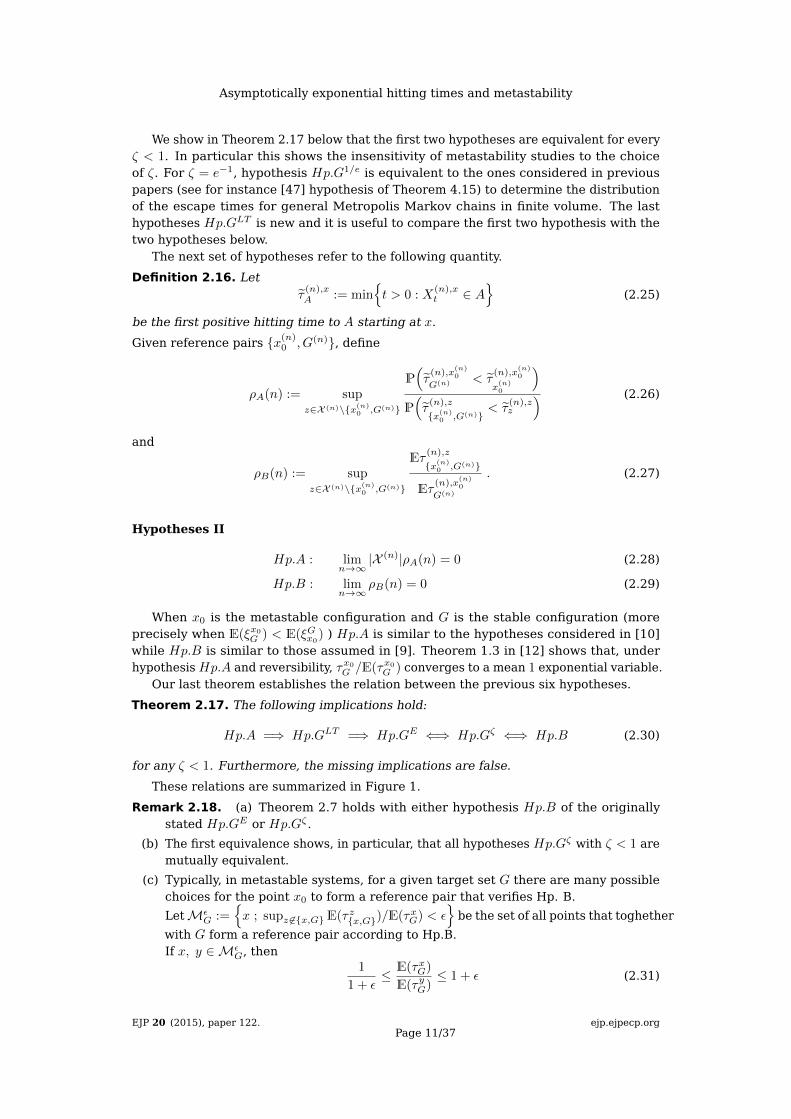
Hp.A =⇒ Hp.GLT =⇒ Hp.GE ⇐⇒ Hp.Gζ ⇐⇒ Hp.B (2.30)

for any ζ < 1. Furthermore, the missing implications are false.

These relations are summarized in Figure 1.

Remark 2.18. (a) Theorem 2.7 holds with either hypothesis Hp.B of the originallystated Hp.GE or Hp.Gζ .

(b) The first equivalence shows, in particular, that all hypotheses Hp.Gζ with ζ < 1 aremutually equivalent.

(c) Typically, in metastable systems, for a given target set G there are many possiblechoices for the point x0 to form a reference pair that verifies Hp. B.

LetMεG :=

{x ; supz 6∈{x,G}E(τz{x,G})/E(τxG) < ε

}be the set of all points that toghether

with G form a reference pair according to Hp.B.If x, y ∈Mε

G, then1

1 + ε≤ E(τxG)

E(τyG)≤ 1 + ε (2.31)

EJP 20 (2015), paper 122./37

ejp.ejpecp.org




Figure 1: Venn diagram for the conditions in theorem 2.17. The two points correspondto particular choices of the parameters in the "abc model" stated in section 5.2.2.

andP (τyx < τyG) ≥ 1− 2ε ; P

(τxy < τxG

)≥ 1− 2ε (2.32)

Indeed, for any x, y, z ∈ X ,

E(τyz ) = E(τy{x,z}) + E(τyz − τy{x,z})

= E(τy{x,z}) + E((τyz − τyx )1τyx<τyz

)= E(τy{x,z}) + E(τxz )P (τyx < τyz ) , (2.33)

where we used strong Markov property at time τyx in the last equality.When x ∈Mε

G,E(τyG) ≤ E(τxG) (ε+ 1) (2.34)

Hence, if both x and y are inMεG, we get the (2.31). From (2.33), by using (2.31)

and x ∈MεG, we get

P (τyx < τyG) =E(τyG)− E(τy{x,G})

E(τxG)≥ 1

1 + ε− ε,

by symmetry, (2.32) follows.

(d) A well-known case is that of finite state space under Metropolis dynamics in thelimit of vanishing temperature. Lemma 3.3 in [16] states that if G is the absoluteminimum of the energy function and x0 is the deepest local minimum, then thereference pair (x0, G) verifies Hp. A.

(e) The implications in Theorem 2.17 are valid for reversible and non-reversible evolu-tions. The counterexamples showing that the missing implications are false, givenin Section 5.2, involve reversible dynamics. This shows that the failure of themissing implications is not associated with lack of reversibility.

3 Key Lemmas

The proofs of the theorems presented in this paper are based on some quite simpleresults on the distribution of the random variable τx0

G . In fact, the central argument is

EJP 20 (2015), paper 122./37

ejp.ejpecp.org




that condition Rec(R, r) implies that renewals –that is, visits to x0– happen at a muchshorter time scale than visits to G. This is expressed through the behavior of thefollowing random times related to recurrence: for each deterministic time u > 0 let

τ∗(u) := inf{s ≥ u : Xs ∈ {x0, G}

}(3.1)

If Y ∼ Exp(1) then the following factorization obviously holds

P(Y > t+ s) = P(Y > t)P(Y > s).

Next lemma controls –for z = x0– this factorization property on a generic time scaleS > R.

Lemma 3.1. If (x0, G) satisfies Rec(R, r), then for any z ∈ X , S > R, t > 0 and s > RS

P(τzG > (t+ s)S

) ≥ [P(τzG > tS +R

)− rP

(τzG > tS

)]P(τx0

G > sS)

≤[P(τzG > tS −R

)+ r]P(τx0

G > sS).

(3.2)

Proof. We start by decomposing according to the time τ∗(tS) to get

P(τzG > (t+ s)S

)= P

(τzG > (t+ s)S ; τ∗(tS) ≤ tS +R

)+ P

(τzG > (t+ s)S ; τ∗(tS) > tS +R

)(3.3)

=

R∑u=0

P(τzG > (t+ s)S ; τ∗(tS) = tS + u

)+

∑x∈{x0,G}c

P(τzG > (t+ s)S ; XtS = x ; τ∗(tS) > tS +R

)We now use Markov property at time tS + u in the first sum, together with the fact thatτzG > τ∗(tS) implies Xτ∗(tS) = x0. In the second sum we use Markov property at instanttS. This yields

P(τzG > (t+ s)S

)=

R∑u=0

P(τ∗(tS) = tS + u ; τzG > tS + u

)P(τx0

G > sS − u)

(3.4)

+∑

x∈{x0,G}cP(τzG > tS ; XtS = x

)P(τxG > sS ; τx{x0,G} > R

).

This identity will be combined with the elementary monotonicity bound with respect to

inclusion{τx0

G > t1} ⊇ {τx0

G > t2} for t1 ≤ t2 , (3.5)

To get the lower bound we disregard the second sum in the right-hand side of (3.4)and bound the first line through the monotonicity bound (3.5) for t1 = tS + u andt2 = tS +R. By condition (2.2) we obtain:

P(τzG > (t+ s)S

)≥ P

(τzG > tS +R ; τ∗(tS) ≤ tS +R

)P(τx0

G > sS)

=[P(τzG > tS +R

)− P

(τzG > tS +R ; τ∗(tS) > tS +R

)]P(τx0

G > sS)

(3.6)

≥[P(τzG > tS +R

)− rP

(τzG > tS

)]P(τx0

G > sS)

EJP 20 (2015), paper 122./37

ejp.ejpecp.org




To get the upper bound in (3.2) exchange s with t in (3.4) and use again the monotonic-ity (3.5) to bound P(τx0

G > tS − u) ≤ P(τx0

G > tS −R) in the first sum in the right-handside. For second sum we use condition (2.2). This yields

P(τzG > (t+ s)S

)≤ P

(τ∗(sS) ≤ sS +R ; τzG > sS

)P(τx0

G > tS −R)

+ P(τzG > sS

)r (3.7)

≤ P(τzG > sS

)[P(τx0

G > tS −R)

+ r].

�

From this “almost factorization”, we can control the distribution of τx0

G on time scaleR. Indeed the following two results are easy consequences of this factorization.

Corollary 3.2. If (x0, G) satisfies Rec(R, r) and S is such that R < S < T := Eτx0

G , then,

P(τx0

G > Sk) ≤[P(τx0

G > S −R) + r]k

(3.8)

P(τx0

G > Sk) ≥[P(τx0

G > S +R)− r]k

(3.9)

for any integer k > 1.

This Corollary immediately follows by an iterative application of Lemma 3.1 witht = 1 and s = k − 1.

Lemma 3.3. If (x0, G) satisfies Rec(R, r), and S is such that R < S < T := Eτx0

G , then

P(τx0

G ≤ S)≤ S +R

T+ r (3.10)

and1

1 + TS−2R

− r ≤ P(τx0

G ≤ S). (3.11)

As a consequence, ∣∣∣P(τx0

G ≤ S)− S

T

∣∣∣ < 2R

T+(ST

)2

+ r . (3.12)

Proof. Let us denote m the integer part of S/R, that is the integer number such that

S −R < mR ≤ S . (3.13)

Proof of the upper bound. We bound the mean time in the form

Eτx0

G =

∞∑t=0

P(τx0

G > t) =

∞∑k=0

(m+1)R(k+1)∑i=(m+1)Rk

P(τx0

G > i)

(3.14)

≤ (m+ 1)R

∞∑k=0

P(τx0

G > (m+ 1)Rk).

The last line is due to the monotonicity property (3.5). Therefore, by (3.8),

Eτx0

G ≤ (m+ 1)R

∞∑k=0

[P(τx0

G > mR)

+ r]k

= (m+ 1)R

∞∑k=0

[1− P

(τx0

G ≤ mR)

+ r]k. (3.15)

EJP 20 (2015), paper 122./37

ejp.ejpecp.org




If P(τx0

G ≤ mR)≤ r the bound (3.10) is trivially satisfied. Otherwise the power series

converges yielding

Eτx0

G ≤ (m+ 1)R

P(τx0

G ≤ mR)− r

and, thus, by (3.13),

P(τx0

G ≤ S)≤ P

(τx0

G ≤ mR)≤ (m+ 1)R

Eτx0

G

+ r ≤ S +R

T+ r . (3.16)

Proof of the lower bound. The argument is very similar, but resorting to the bound

Eτx0

G =

∞∑k=0

(m−1)R(k+1)∑i=(m−1)Rk

P(τx0

G > i)≥ (m− 1)R

∞∑k=0

P(τx0

G > (m− 1)R(k + 1))

≥ (m− 1)R

∞∑k=0

P(τx0

G > (S −R)(k + 1))≥ (m− 1)R

∞∑k=1

[P(τx0

G > S)− r]k.

The second and third inequalities follow from monotonicity, while the last one is dueto the lower bound (3.9). The power series is converging because

∣∣P(τx0

G > S)− r∣∣ < 1

since r ∈ (0, 1). Its sums yields

Eτx0

G

(m− 1)R≥ 1

P(τx0

G ≤ S)

+ r− 1 ,

so that

P(τx0

G ≤ S)≥ 1

1 + TS−2R

− r (3.17)

in agreement with (3.11)s. �

Remark 3.4. The error term r becomes exponentially small as the recurrence parameterR is increased linearly. More precisely, if Rec(R, r) holds then

supx∈X

P(τx{x0,G} > NR

∣∣∣ τx{x0,G} > (N − 1)R)≤ r , (3.18)

which implies,

supx∈X

P(τx{x0,G} > NR

)≤ rN . (3.19)

In particular, for T � R we can replace R by R+ := NR. For this reason we can assumein what follows r < ε.

The bounds given in the preceding lemmas, however, are not enough for our purposes.To control large values of S with respect to T (tail of the distribution), we need topass from additive to multiplicative errors, that is from bounds on

∣∣P(τx0

G > S +R)−

P(τx0

G > S)∣∣ to bounds on P

(τx0

G > S +R) /

P(τx0

G > S). Our bounds will be in terms of

the following parameters.

Definition 3.5. Let c, c̄ be

c := P(τx0

G ≤ 2R) + r (3.20)

and

c̄ :=

12 −

√14 − c if c ≤ 1

4

1 if c > 14

(3.21)

EJP 20 (2015), paper 122./37

ejp.ejpecp.org




We shall work in regimes where these parameters are small. Note that, by Lemma3.3, hypothesis Rec(R, r) implies that

c < 3R

T+ 2r . (3.22)

Moreover, in the case c < 1/4 definition (3.21) is equivalent to

c = c̄(1− c̄) < c̄ . (3.23)

Our bounds rely on the following lemma, which yields control on the tail density ofτx0

G .

Lemma 3.6. Let (x0, G) be a reference pair satisfying Rec(R, r) and S > R, then, forany z ∈ X ,

P(τzG ≤ S +R

)≤ P

(τzG ≤ S

) [1 +

c

P(τzG ≤ S

)] (3.24)

Furthermore, if z ∈ B(x0, c̄− c),

P(τzG > S +R

)≥ P

(τzG > S

)[1− c− c̄] . (3.25)

Proof.Proof of (3.24). We decompose

P(τzG ≤ S +R

)= P

(τzG ≤ S

)+ P

(τzG ∈ (S, S +R)

)= P

(τzG ≤ S

)+ P

(τzG ∈ (S, S +R), τ∗(S −R) ≤ S

)+ P

(τzG ∈ (S, S +R), τ∗(S −R) > S

). (3.26)

The event{τzG ∈ (S, S + R), τ∗(S − R) < S

}corresponds to having a visit to x0 in

the interval [S − R,S] followed by a first visit to G is in the interval (S, S + R). ByMarkovianness,

P(τzG ∈ (S, S +R), τ∗(S −R) ≤ S

)=

∑u∈[S−R,S]v∈(S,S+R]

P(Xu = x0 ; τzG ≥ u ; Xi 6∈ G, u < i < v ; Xv ∈ G

)(3.27)

=∑

u∈[S−R,S]v∈(S,S+R]

P(Xu = x0 , τ

zG ≥ u

)P(τx0

G = v − u).

Hence, by monotonicity,

P(τzG ∈ (S, S +R), τ∗(S −R) ≤ S

)≤ P

(τzG > S −R

)P(τx0

G ≤ 2R). (3.28)

Analogously, Markovianness and monotonicity yield

P(τzG ∈ (S, S +R), τ∗(S −R) > S

)=

∑x 6∈{x0,G}

P(τzG ∈ (S, S +R) ; XS = x ; Xi 6∈ {x0, G}, S −R < i ≤ S

)(3.29)

≤ P(τzG > S −R

)sup

x 6∈{x0,G}P(τx{x0,G} > R

).

EJP 20 (2015), paper 122./37

ejp.ejpecp.org




Hence, by condition Rec(R, r) and monotonicity,

P(τzG ∈ (S, S +R), τ∗(S −R) > S

)< P

(τzG > S −R

)r . (3.30)

Inserting (3.28) and (3.30) in (3.26) we obtain

P(τzG ≤ S +R

)≤ P

(τzG ≤ S

)+[P(τx0

G ≤ 2R)

+ r]P(τzG > S −R

). (3.31)

The bound (3.24) is obtained by recalling (3.20) and by neglecting the last term.

Proof of (3.25). If c > 1/4 there is nothing to prove. For c ≤ 1/4 we perform, for each z,a decomposition similar to (3.26):

P(τzG > S +R

)= P

(τzG > S

)− P

(τzG ∈ (S, S +R)

)= P

(τzG > S

)− P

(τzG ∈ (S, S +R), τ∗(S −R) < S

)(3.32)

− P(τzG ∈ (S, S +R), τ∗(S −R) ≥ S

).

The bounds (3.28) and (3.30) yield

P(τxG > S +R

)≥ P

(τzG > S

)− P

(τzG > S −R

)[P(τx0

G ≤ 2R)

+ r]

which can be written as

P(τzG > S +R

)P(τzG > S

) ≥ 1− cP(τzG > S −R

)P(τzG > S

) . (3.33)

Let us first consider the case in which S = iR for an integer i. Denote

yi =P(τzG > (i+ 1)R

)P(τzG > iR

) , (3.34)

so condition (3.33) becomesyi ≥ 1− c

yi−1(3.35)

The proposed inequality (3.25) follows from the followingClaim:

yi > 1− c̄ (3.36)

We prove this by induction. For i = 0, we first notice that

P(τzG ≤ 2R

)= P

(τzG ≤ 2R , τzx0

≥ R)

+ P(τzG ≤ 2R , τzx0

< R)≤ P

(τz{x0,G} 6= τzx0

)+P(τz{x0,G} = τzx0

≥ R, τzG ≤ 2R)

+

R−1∑u=0

P(τzG > u , τzx0

= u)P(τx0

G ≤ 2R− u).

The last inequality results from Markovianness and monotonicity. Hence, if z ∈ B(x0, r0)

P(τzG ≤ 2R

)≤ r0 + r + P

(τx0

G ≤ 2R). (3.37)

where we used (2.9). As a consequence, using the definition of c, if r0 < c− c̄,

y0 = 1− P(τzG ≤ R

)≥ 1− P

(τzG ≤ 2R

)≥ 1− c− r0 > 1− c̄ .

EJP 20 (2015), paper 122./37

ejp.ejpecp.org




and the claim holds. Assume now that the claim is true for i, then, by (3.35) and theinductive hypothesis,

yi+1 ≥ 1− c

yi> 1− c

1− c̄= 1− c̄. (3.38)

The last identity follows from the equality in (3.23). The claim is proven.

To conclude we consider the case in which kR ≤ S ≤ (k + 1)R, with k = b SRc. Bymonotonicity,

P(τzG > S +R

)≥ P

(τzG > (k + 2)R

), P

(τzG > kR

)≥ P

(τzG > S

)Then, by the previous claim and the definition of c̄,

P(τzG > S +R

)P(τzG > S

) ≥P(τzG > (k + 2)R

)P(τzG > kR

) = yk+1 yk > (1− c̄)2 = 1− c̄− c . (3.39)

This conclude the proof of (3.25). �

Remark 3.7. When c is small Lemma 3.6 implies that the distribution of τx0

G does notchange very much passing from S to S + R. We have to note that the control here

is given by estimating near to one the ratiosP

(τx0G >S+R

)P

(τx0G >S

) andP

(τx0G ≤S+R

)P

(τx0G ≤S

) , providing

in this way a “multiplicative error" on the distribution function. In general such anestimate is different and more difficult w.r.t. an estimate with an “additive error", i.e.,

which amounts to show that the difference |P(τx0

G > S +R)− P

(τx0

G > S)| is near to

zero. The estimate with a multiplicative error is crucial when considering the tail ofthe distribution, since in Lemma 3.6 there are no upper restriction on S. Similarly in

(3.24) the estimate onP

(τx0G ≤S+R

)P

(τx0G ≤S

) is relevant for S not too small when we can prove, by

Lemma 3.3, that cP(τ

x0G ≤S)

is small. Note also that the last term in (3.24) is small due to

Lemma 3.3.

We use this lemma to prove a multiplicative-error strengthening of Lemma 3.1.

Lemma 3.8. Let (x0, G) be a reference pair satisfying Rec(R, r), S > R and r and c sothat

r + c+ c̄ < 1 . (3.40)

Then, for any z ∈ B(x0, r),

P(τzG > (t+ s)S

)P(τzG > tS

)P(τx0

G > sS) ≥ 1− (c+ c̄+ r) . (3.41)

and, for any z ∈ X

P(τzG > (t+ s)S

)P(τzG > tS

)P(τx0

G > sS) ≤ 1 +

c+ c̄+ r

1− (c+ c̄+ r)(3.42)

Proof. Inequality (3.41) is a consequence of the top inequality in Lemma 3.1 andinequality (3.25) of Lemma 3.6.

To prove (3.42) we resort to the decomposition (3.4) which we further decompose bywriting {

τxG > sS ; τxx0,G > R}

=

bsS/Rc⋃n=1

{τxG > sS ; τxx0,G ∈ Vn

}, (3.43)

EJP 20 (2015), paper 122./37

ejp.ejpecp.org




with

Vn =

{ (nR, (n+ 1)R

]1 ≤ n ≤ bsS/Rc − 1

(nR,∞) n = bsS/RcWe obtain,

P(τzG > (t+ s)S

)=

R∑u=0

P(τ∗(tS) = tS + u ; τzG > tS + u

)P(τx0

G > sS − u)

(3.44)

+∑

x∈{x0,G}cP(τzG > tS ; XtS = x

) bsS/Rc∑n=1

P(τxG > sS ; τxx0,G ∈ Vn

)and, by monotonicity,

P(τzG > (t+ s)S

)≤ P

(τzG > tS

)P(τx0

G > sS −R)

(3.45)

+ P(τzG > tS

) bsS/Rc∑n=1

supx∈{x0,G}c

P(τxG > sS ; τxx0,G ∈ Vn

).

Markovianness and monotonicity imply the following bounds,

P(τxG > sS, τxx0,G ∈ Vn

)≤

∑u∈Vn

P(τxx0

= u ; τx0

G ≥ sS − u)

≤∑u∈Vn

P(τxx0

= u)P(τx0

G ≥ sS − u)≤ P

(τx{x0,G} > nR

)P(τx0

G ≥ sS − nR).(3.46)

Hence, using bounds (3.19) and (3.25),

P(τxG > sS, τxx0,G ∈ Vn

)≤ rn

P(τx0

G ≥ sS)

(1− c− c̄)n. (3.47)

Replacing this into (3.45) yields

P(τzG > (t+ s)S

)≤ P

(τzG > sS

)P(τx0

G > tS −R)

+ P(τzG > sS

)P(τx0

G > tS) ∞∑n=1

( r

1− c− c̄

)n≤ P

(τzG > sS

)P(τx0

G > tS)[ 1

1− c− c̄+

a

1− a

](3.48)

with a = r/(1− c− c̄). [We used (3.25) in the first summand.] Equation (3.41) follows bynoting that[ 1

1− c− c̄+

a

1− a

]= 1 +

c+ c̄

1− c− c̄+

r

1− c− c̄− r≤ 1 +

c+ c̄+ r

1− c− c̄− r. �

The preceding lemma implies the following improvement of Corollary 3.2:

Corollary 3.9. Let (x0, G) be a reference pair satisfying Rec(R, r), and let r and c besufficiently small so that r + c+ c̄ < 1

2 and define

δ0 := ln[1 +

c+ c̄+ r

1− (c+ c̄+ r)

](3.49)

Then, for S > R and k = 1, 2, . . .

e−δ0 k ≤P(τx0

G > kS)

P(τx0

G > S)k ≤ eδ0 k . (3.50)

EJP 20 (2015), paper 122./37

ejp.ejpecp.org




The inequalities are just an iteration of (3.41) and (3.42). In fact, the left inequalitycan be extended to any z ∈ B(x0, r) and the right inequality to any z ∈ X . We will notneed, however, such generality.

The multiplicative bounds of Lemma 3.8 can be transformed into bounds for z inB(x0, r) with the help of the following lemma.

Lemma 3.10. Consider a reference pair (x0, G), with x0 ∈ X , such that Rec(R, r) holdswith R < T := Eτx0

G .For all z ∈ B(x0, r0)

P(τzG > tT

)≥ P

(τx0

G > tT)

(1− r − r0) . (3.51)

Proof. This is proven with a decomposition similar to those used in the proof of Lemma3.8. We have:

P(τzG > tT

)≥ P

(τzG > tT, τz{x0,G} < R

)=

R∑u=0

P(τzG > tT, τz{x0} = u

)=

R∑u=0

P(τzG > u, τz{x0} = u

)P(τx0

G > tT − u)

The last identity is due to Markovianness at u. By monotonicity, we conclude

P(τzG > tT

)≥ P

(τx0

G > tT)P(τz{x0,G} ≤ R, τ

z{x0,G} = τz{x0}

)= P

(τx0

G > tT) [

1− P({τz{x0,G} > R

}∪{τz{x0,G} 6= τz{x0}

})]which implies (3.51).�

The bound (3.51) is complemented by the bound

P(τzG > tT

)≤ P

(τx0

G > tT)

(1 + r) (3.52)

implied by the bottom inequality in (3.2). Combined with Lemma 3.8, the bounds (3.51)and (3.52) yield the bound

1− (c+ c̄+ r)

1 + r≤

P(τzG > (t+ s)S

)P(τzG > tS

)P(τzG > sS

) ≤ 1 + c+c̄+r1−(c+c̄+r)

1− r − r0(3.53)

valid for all z ∈ B(x0, r0) when c, r and r0 are so small that c + c̄ + r < 1, r0 ≤ r andr + r0 < 1.

4 Proofs on exponential behaviour

4.1 Proof of Theorem 2.3

We chose an intermediate time scale S, with R < S < T . While this scale will finallybe related to ε and r, for the sake of precision we introduce an additional parameter

η :=S

T, 0 < ε < η < 1 . (4.1)

To avoid trivialities in the sequel, we assume that η, ε and r are small enough so that

c+ c̄+ r < 1/2 and η + ε+ r < 1 . (4.2)

We decompose the proof into nine claims that may be of independent interest. Theclaims provide bounds for ratios of the form P

(τx0

G > η t)/e−t from which bounds for∣∣P(τx0

G > η t)− e−t

∣∣ can be readily deduced.

EJP 20 (2015), paper 122./37

ejp.ejpecp.org




Claim 1: Bounds for t = η.

e−η α1 ≤P(τx0

G > η T)

e−η≤ eη α0 (4.3)

with

α0 := 1 +1

ηlog[ 1

1 + η − 2ε+ r]

α1 := −1− 1

ηlog(1− η − ε− r

). (4.4)

This is just a rewriting of the bounds (3.10) and (3.11) as shown by the following chainof inequalities:

e−η[1+α1] := 1− η − ε− r ≤ P(τx0

G > η T)≤ 1− η − 2ε

η − 2ε+ 1+ r =: e−η[1−α0] . (4.5)

Note that, as η, ε and r tend to zero,

α0 , α1 = O(ε/η) +O(r/η) . (4.6)

Claim 2: Bounds for all ε < t < η,

C(1)− e−t α1 ≤

P(τx0

G > tT)

e−t≤ C

(1)+ et α0 (4.7)

with functions C(1)± (η, ε, r) = 1 +O(η) +O(ε) +O(r) . Indeed, inequalities (4.5) hold also

with η replaced by t and yield

e−tα1 et[α1−αt1] = e−t αt1 ≤

P(τx0

G > tT)

e−t≤ et α

t0 = et α0 et[α

t0−α0] (4.8)

where αt0 and αt1 are defined as in (4.4) but with t replacing η. This is precisely (4.7) with

C(1)+ = sup

ε<t≤ηet[α

t0−α0] = sup

ε<t≤η

(1 + t− 2ε)−1 + r[(1 + η − 2ε)−1 + r

]t/η (4.9)

and

C(1)− = inf

ε<t≤ηet[α1−αt1] = inf

ε<t≤η

[1− η − ε− r

]t/η1− t− ε− r

. (4.10)

Claim 3: Bounds for all t ≤ ε,

C(0)− e−t α1 ≤

P(τx0

G > tT)

e−t≤ C

(0)+ et α0 , (4.11)

with functions C(0)± (η, ε, r) = 1+O(η)+O(ε)+O(r) . Indeed, the restriction t ≤ ε implies

that1− (2ε+ r) ≤ P

(τx0

G > εT)≤ P

(τx0

G > tT)≤ 1 , (4.12)

where the leftmost inequality is a consequence of (3.10) plus the right continuity ofprobabilities. The upper bound in (4.11) is a consequence of the rightmost inequality in(4.12) and the inequalities

P(τx0

G > tT)

e−t≤ et ≤ eε ≤ eε et α0 = C

(0)+ et α0 (4.13)

EJP 20 (2015), paper 122./37

ejp.ejpecp.org




with C(0)+ = eε. The lower bound in (4.11), in turns, follows form the leftmost inequality

in (4.12) and the inequalities

P(τx0

G > tT)

e−t≥ et

[1− (2ε+ r)

]≥ e−t α1

[1− (2ε+ r)

]= C

(0)− e−t α1 (4.14)

with C(0)− = 1− (2ε+ r).

Putting the preceding three claims together we readily obtain

Claim 4: Bounds for all t ≤ η,

C− e−t α1 ≤

P(τx0

G > tT)

e−t≤ C+ e

t α0 , (4.15)

with functions C±(η, ε, r) = 1 +O(η) +O(ε) +O(r). Indeed, this follows from the threepreceding claims, putting

C+ = max{C

(0)+ , C

(1)+

}, C− = min

{C

(0)− , C

(1)−}. (4.16)

Claim 5: Bounds for t = kη. Let δ0 be as in Corollary 3.9, then for any integer k ≥ 1,

e−k η λ1 ≤P(τx0

G > k η T)

e−k η≤ ek η λ0 (4.17)

with

λ0 = α0 +δ0η, λ1 = α1 +

δ0η. (4.18)

This result amounts to putting together (3.50) and (4.3). Notice that —by (3.21)–(3.22)— c, c̄ = O(ε) +O(r), hence from (4.6) and the definition (3.49) of δ0,

λ0 , λ1 = O(ε/η)

+O(r/η). (4.19)

Claim 6: Bounds for any t > 0,

C− e−t λ1 ≤

P(τx0

G > tT)

e−t≤ C+ e

t λ0 (4.20)

with

C+ = C+

[1 +

c+ c̄+ r

1− (c+ c̄+ r)

], C− = C−

[1− (c+ c̄+ r)

]. (4.21)

Indeed, for any t > 0 there exist an integer k ≥ 0 and 0 ≤ t′ < η such that t = k η + t′.Hence,

P(τx0

G > tT)

e−t=

P(τx0

G > (k η + t′)T)

P(τx0

G > k η T)P(τx0

G > t′ T) P

(τx0

G > k η T)

e−k η

P(τx0

G > t′ T)

e−t′(4.22)

and the claim follows from (3.41). (3.42), (4.15) and (4.17).

Claim 7: The bounds (4.20) implies the bound (2.5) for any t > 0.Indeed, subtracting 1 and multiplying through by e−t, (4.20) implies∣∣∣P(τx0

G > tT)− e−t

∣∣∣ ≤ C e−t (4.23)

EJP 20 (2015), paper 122./37

ejp.ejpecp.org




withC = max

{(C+ e

t λ0 − 1),∣∣1− C− e−t λ1

∣∣} . (4.24)

To conclude the proof we notice that C+ , C− = 1 + O(η) + O(ε) + O(r) and, hence,by (4.19),

C = O(η) +O(ε/η) +O(r/η) . (4.25)

At this point we choose η appropriately to satisfy the asymptotic behavior (2.4). Ademocratic choice, that makes the different contributions of comparable size is

η =√

max{ε, r} . (4.26)

Claim 8: Let r0 be such that r + r0 < 1. Then for any z ∈ B(x0, r0) and any t > 0,

C̃− e−t λ1 ≤

P(τzG > tT

)e−t

≤ C̃+ et λ0 (4.27)

with

C̃+ = C+

[1 +

c+ c̄+ r

1− (c+ c̄+ r)

]C̃− = C−

(1− r − r0

). (4.28)

Indeed, the upper bound follows from the upper bound in (4.20) and (3.42) with thesubstitutions S → T , t = 0 and s → t. The lower bound is a consequence of the lowerbound in (4.20) and (3.51) in Lemma 3.10 This concludes also the proof of (2.7). �

4.2 Proof of Theorem 2.7:

Part (I). The results follow from (2.5) and (2.7) by letting both εn := Rn /Eτ(n),x

(n)0

G(n) andrn tend to zero.

Part (II) (i). Let

ϑn :=τ

(n),x(n)0

G(n)

Qn(ζ). (4.29)

Combining the definition (2.11) of Qn(ζ) with Corollary 3.9 we obtain[ζ e−δ0,n

]k ≤ P(ϑn > k

)≤[ζ eδ0,n

]k(4.30)

withδ0,n −→ 0 as εn, rn → 0 . (4.31)

A simple argument based on Markov inequality [see (5.2)–(5.3) below] shows thathypothesis Hp.G(Qn(ζ)) implies hypothesis Hp.G(Tn) [in fact, they are equivalent, asshown in Theorem 2.17]. Hence, (4.31) holds under hypothesis Hp.G(Qn(ζ)) and (4.30)shows that the sequence of random variables (ϑn) is exponentially tight. Therefore, thesequence is relatively compact in the weak topology (Dunford-Pettis theorem) and everysubsequence has a sub-subsequence that converges in law. Let (ϑnk)k be one of theseconvergent sequences and let ϑ be its limit. Taking limit in (3.2) we see that

P(ϑ > t+ s) = P(ϑ > t)P(ϑ > s) (4.32)

for all continuity points s, t > 0. Since these points are dense and the distributionfunction is right-continuous, (4.32) holds for all s, t ≥ 0. Furthermore, the limit of (4.30)implies that

P(ϑ > k

)= ζk . (4.33)

We conclude that ϑ is an exponential variable of rate − log ζ. As every subsequence of(θn) converges to the same exp(− log ζ) law, the whole sequence does.

EJP 20 (2015), paper 122./37

ejp.ejpecp.org




Part (II) (ii). The rightmost inequality in (4.30) implies that fixing ζ < ζ̃ < 1, we havethat for n large enough

P(ϑn > k

)≤ ζ̃k

for all k ≥ 1. By monotonicity this implies that

P(ϑn > t

)≤ ζ̃btc (4.34)

for n large enough. As the function in the right-hand side is integrable, we can applydominated convergence and conclude:

limn→∞

Qn(ζ)

TEn= lim

n→∞

∫ ∞0

P(ϑn > t

)dt =

∫ ∞0

P(ϑ > t

)dt = − ln ζ . � (4.35)


We assume ε and r small enough so that c+ c̄+ r < 1/2. We shall produce an upperand a lower bound for the ratio

REE(S) :=P(τx0

G ∈ (kS, (k + 1)S))

P(τx0

G > S)kP(τx0

G ≤ S) (4.36)

for k < T/S. We start with the identity

P(τx0

G ∈ (kS, (k + 1)S))

= P(τx0

G ∈ (kS, (k + 1)S), τ∗(kS −R) ≤ kS)

+ P(τx0

G ∈ (kS, (k + 1)S), τ∗(kS −R) > kS)

(4.37)

Applying Markov property and monotonicity we obtain the upper bound

P(τx0

G ∈ (kS, (k + 1)S))≤ P

(τx0

G > kS −R)P(τx0

G ≤ R+ S)

+ P(τx0

G > kS −R)r (4.38)

and the lower bound

P(τx0

G ∈ (kS, (k + 1)S))≥ P

(τx0

G > kS)P(τx0

G ≤ S)− P

(τx0

G > kS)r . (4.39)

This lower bound and the leftmost inequality in (3.50) yields the lower bound

REE(S) ≥

P(τx0

G > kS)P(τx0

G ≤ S)[

1− r

P

(τx0G ≤S

)]

P(τx0

G > S)kP(τx0

G ≤ S)

≥ e−δ0k[1− r

P(τx0

G ≤ S)] . (4.40)

To obtain a bound in the opposite direction we use the upper bound (4.38):

REE(S) ≤P(τx0

G > kS −R)[P(τx0

G ≤ R+ S)

+ r]

P(τx0

G > S)kP(τx0

G ≤ S) . (4.41)

EJP 20 (2015), paper 122./37

ejp.ejpecp.org




We bound the right-hand side through the rightmost inequality in (3.50) and the followingtwo easy consequences of (3.25):

P(τx0

G > kS −R)≤P(τx0

G > kS)

1− c− c̄(4.42)

[obtained by replacing S → kS −R in (3.25)] and

P(τx0

G ≤ R+ S)≤ P

(τx0

G ≤ S)

(1 + c+ c̄) . (4.43)

The result is

REE(S) ≤ 1

1− c− c̄eδ0k

[1 + c+ c̄+

r

P(τx0

G ≤ S)] (4.44)

Inspection shows that the dominant order in both bounds (4.40) and (4.44) is givenby the term

r

P(τx0

G ≤ S) ≤ r

1− e−η(1−α0), (4.45)

the last inequality being a consequence of the rightmost inequality in (4.3). From (4.4)we see that

r

1− e−η(1−α0)=

r

O(η) +O(ε) +O(r)= O

(ε/η)

+O(r/η). (4.46)

With this observation, the bounds (4.40) and (4.44) imply∣∣REE(S)− 1∣∣ ≤ O

(ε/η)

+O(r/η). � (4.47)

5 Proof of the relation between different hypotheses for exponen-tial behavior

In subsection 5.1 we prove Theorem 2.17 and in subsection 5.2.2 we give examplesthat show that the converse of each of the first two implications in (2.30) are false.


(i) Hp.A⇒ Hp.GLT : By Markovianness, if x 6= y ∈ X ,

P(ξxy (x) > t) = P(ξxy (x) > t− 1)P(ξxy (x) ≥ 1) = P(ξxy (x) > t− 1)P(τ̃xy > τ̃xx ) ,

thusP(ξxy (x) > t) = P(τ̃xy > τ̃xx )t

andE(ξxy (x)) = P(τ̃xy < τ̃xx )−1.

Therefore,

ρA(n) =supz∈{x0,G}c E

(ξz{x0,G}(z)

)E(ξx0

G (x0)) =

supz∈{x0,G}c E(ξz{x0,G}(z)

)TLTn

. (5.1)

Furthermore, by Markov inequality

P(τz{x0,G} > Rn

)= P

( ∑x∈{x0,G}c

ξz{x0,G}(x) > Rn

)

≤

∑x∈{x0,G}c E

(ξx{x0,G}(x)

)Rn

≤ |X | ρA(n)TLTnRn

.

EJP 20 (2015), paper 122./37

ejp.ejpecp.org




The proposed implication follows, for instance, by choosing Rn = εnTLTn with εn =√

|X |ρA(n).

(ii) Hp.GLT ⇒ Hp.GE: It is an immediate consequence of the obvious inequalityTEn > TLTn .

(iii) Hp.GE ⇐ Hp.GQ(ζ): By Markov inequality,

P(τx0

G > t)≤E(τx0

G

)t

. (5.2)

Thus,TQ(ζ)n ≤ ζ−1 TEn . (5.3)

(iv) Hp.GE ⇒ Hp.GQ(ζ): We bound:

E(τx0

G

)=∑k≥0

∑kTQ

ζn ≤t<(k+1)TQ

ζn

P(τx0

G > t)≤ TQ(ζ)

n

∑k≥0

P(τx0

G > k TQ(ζ)n

).

Hence, by Lemma 3.9,

TEn ≤ TQ(ζ)n

[1 +O

((ζ + εn + rn)

)]. (5.4)

(v) Hp.GE ⇐ Hp.B: Apply the Markov inequality to P(τx{x0,G} > Rn) and choose

Rn =√TEn supz∈{x0,G}c E(τz{x0,G}).

(vi) Hp.GE ⇒ Hp.B:

supz∈{x0,G}c

E(τz{x0,G}) = supz∈{x0,G}c

∑t≥0

P(τz{x0,G} > t) ≤ Rn +Rn supz∈{x0,G}c

∞∑N=1

P(τz{x0,G} > NRn)

≤ Rn +Rn

∞∑N=1

supz∈{x0,G}c

P(τz{x0,G} > Rn)N ≤ Rn +Rn

1− rn≤ const. Rn

As Hp.GE implies Rn ≺ TEn we obtain that ρB(n)→ 0. �

5.2 Counterexamples

5.2.1 h model (freedom of starting point)

We show that even in the finite–volume case the set of starting points that verify Hp. B isin general bigger than the set of good starting points for Hp. A and that these are notlimited to the deepest local minima of the energy.

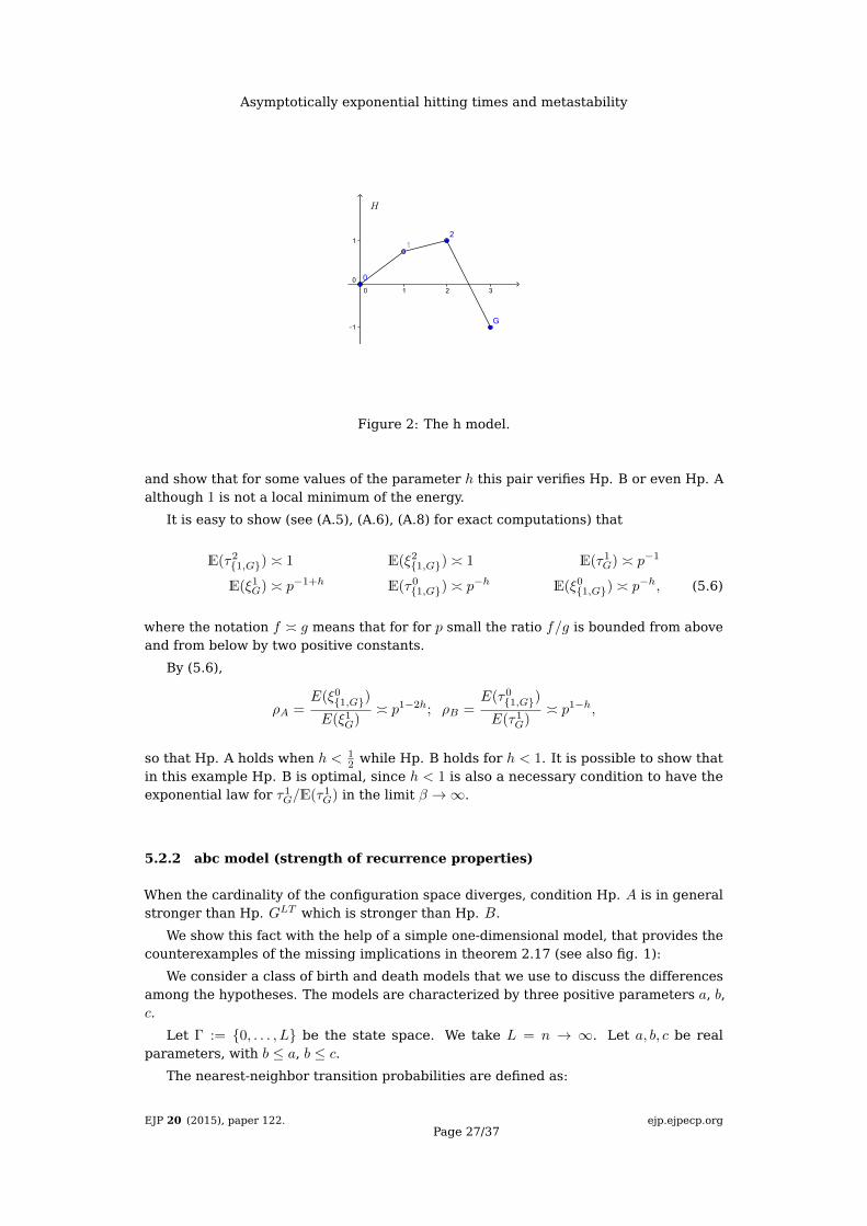
Let us consider a birth-and-death model with state space {0, 1, 2, G} and transitionmatrix

P (0, 1) :=1

2ph P (1, 2) :=

1

2p1−h P (1, 0) :=

1

2

P (2, G) :=1

2P (2, 1) :=

1

2P (G, 2) :=

1

2p2 (5.5)

and P (i, i) = 1−∑j 6=i P (i, j) for i ∈ {0, 1, 2, G}. This model can be seen as a Metropolis

chain with energy function H(0) = 0, H(1) = h, H(2) = 1, H(G) = −1 (see fig. 2).By Lemma 3.3 in [16], the reference pair (0, G) always fulfils Hp. A (and thus Hp. B),

since 0 is the most stable local minimum of the energy. We focus here on the pair (1, G)

EJP 20 (2015), paper 122./37

ejp.ejpecp.org




Figure 2: The h model.

and show that for some values of the parameter h this pair verifies Hp. B or even Hp. Aalthough 1 is not a local minimum of the energy.

It is easy to show (see (A.5), (A.6), (A.8) for exact computations) that

E(τ2{1,G}) � 1 E(ξ2

{1,G}) � 1 E(τ1G) � p−1

E(ξ1G) � p−1+h E(τ0

{1,G}) � p−h E(ξ0

{1,G}) � p−h, (5.6)

where the notation f � g means that for for p small the ratio f/g is bounded from aboveand from below by two positive constants.

By (5.6),

ρA =E(ξ0

{1,G})

E(ξ1G)

� p1−2h; ρB =E(τ0

{1,G})

E(τ1G)

� p1−h,

so that Hp. A holds when h < 12 while Hp. B holds for h < 1. It is possible to show that

in this example Hp. B is optimal, since h < 1 is also a necessary condition to have theexponential law for τ1

G/E(τ1G) in the limit β →∞.

5.2.2 abc model (strength of recurrence properties)

When the cardinality of the configuration space diverges, condition Hp. A is in generalstronger than Hp. GLT which is stronger than Hp. B.

We show this fact with the help of a simple one-dimensional model, that provides thecounterexamples of the missing implications in theorem 2.17 (see also fig. 1):

We consider a class of birth and death models that we use to discuss the differencesamong the hypotheses. The models are characterized by three positive parameters a, b,c.

Let Γ := {0, . . . , L} be the state space. We take L = n → ∞. Let a, b, c be realparameters, with b ≤ a, b ≤ c.

The nearest-neighbor transition probabilities are defined as:

EJP 20 (2015), paper 122./37

ejp.ejpecp.org




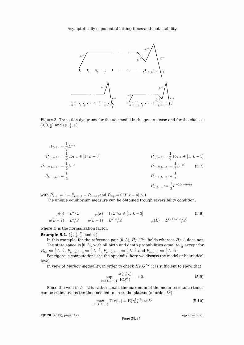
Figure 3: Transition dyagrams for the abc model in the general case and for the choices(0, 0, 3

2 ) and ( 34 ,

14 ,

74 ).

P0,1 : =1

2L−a

Px,x+1 : =1

2for x ∈ [1, L− 3] Px,x−1 :=

1

2for x ∈ [1, L− 3]

PL−2,L−1 : =1

2L−c PL−2,L−3 :=

1

2L−b (5.7)

PL−1,L : =1

2PL−1,L−2 :=

1

2

PL,L−1 :=1

2L−2(a+b+c)

with Px,x := 1− Px,x−1 − Px,x+1and Px,y = 0 if |x− y| > 1.The unique equilibrium measure can be obtained trough reversibility condition:

µ(0) = La/Z µ(x) = 1/Z ∀x ∈ [1, L− 3] (5.8)

µ(L− 2) = Lb/Z µ(L− 1) = Lb−c/Z µ(L) = L2a+3b+c/Z,

where Z is the normalization factor.

Example 5.1. (58 ,14 ,

74 model )

In this example, for the reference pair (0, L), Hp.GLT holds whereas Hp.A does not.The state space is [0, L], with all birth and death probabilities equal to 1

2 except for

P0,1 := 12L− 5

8 , PL−2,L−3 := 12L− 1

4 , PL−2,L−1 := 12L− 7

4 and PL,L−1 := 12L− 21

2 .For rigorous computations see the appendix, here we discuss the model at heuristical

level.In view of Markov inequality, in order to check Hp.GLT it is sufficient to show that

supx∈{1,L−1}

E(τx0,L)

E(ξ0L)−→ 0. (5.9)

Since the well in L− 2 is rather small, the maximum of the mean resistance timescan be estimated as the time needed to cross the plateau (of order L2):

maxx∈{1,L−1}

E(τx0,L) = E(τL−20,L ) � L2 (5.10)

EJP 20 (2015), paper 122./37

ejp.ejpecp.org




(see (A.25) for a rigorous computation).The mean local time can be estimated by using (A.12): the probability that the

process starting from 0 visits L before returning to 0 can be estimated as the probabilityof stepping out from 0 (which is P0,1 = 1

2L− 5

8 ) times the probability of reaching L − 2

before returning (which is of order L−1) times the probability that the process startingfrom L− 2 visits L before 0 (which is of order L

54 /L

74 ). The mean local time of 0 (i.e. the

time spent in 0 before the visit to L) is therefore

E(ξ0L) = P

(τ̃0L < τ̃0

0

)−1

=(P0,1P

(τ̃1L−2 < τ̃1

0

)P(τ̃L−2L < τ̃L−2

0

))−1 � L 58 +1+ 1

2 = L178 (5.11)

(as proven in (A.12)). Thus, by (5.10), (5.11) the ratio in (5.9) goes like � L−18 and

condition Hp.GLT holds.On the other hand, the maximum of the mean local time before hitting 0 or L is

reached in L− 2 and it is of the order of the inverse of PL−2,L−3 (i.e. the probability ofexiting from L− 2) times the probabily of exiting the plateau in 0 (of order L−1):

maxx∈[1,L−1]

E(ξx0,L) = E(ξL−20,L ) �

(PL−2,L−3P

(τ̃L−30 < τ̃L−3

L−2

))� L 5

4 (5.12)

(see (A.14) for particulars). Thus, by (5.11), (5.12),

LρA(L) � L L54

L178

= L18 −→∞ (5.13)

that is, condition A does not hold.

Example 5.2. (0,0, 32 model )This choice of parameters corresponds to a birth-and-death chain where all birth and

death probabilities are set equal to 12 except for PL−2,L−1 := 1

2L− 3

2 and PL,L−1 := 12L−3.

We show that, for the reference pair (0, L), condition Hp.B holds whereas conditionHp.GLT does not.

Precise computations can be found in the appendix, here we discuss the model atheuristic level.

We start by estimating ρB(L) := supz<LE(τz0,L)/E(τ0L):

Each time the process is in L − 2, it has a probability 12L− 3

2 of reaching L in twosteps, but the probability to find the process in L − 2 before the transition is of orderL−1; hence,

E(τ0L) � L× L 3

2 ,

see eq. (A.16) for the exact computation.The maximum of the mean times is dominated by a diffusive contribution:

maxx∈[1,L−1]

E(τx0,L) = E(τL−20,L ) � L2,

as confirmed by (A.25).Thus, ρB � L−

12 and condition B holds.

Next, we show that

P(τL/2{0,L} > E(ξ0

L))−→ 1, (5.14)

and, therefore, that Hp.GLT does not hold.Equation (A.12) allows to compute the mean local time: The probability that the

process starting from 0 visits L before returning to 0 can be estimated as the probability

EJP 20 (2015), paper 122./37

ejp.ejpecp.org




of reaching L− 2 before returning (which is of order L−1) times the probability that theprocess starting from L− 2 visits L before 0 (which is of order L/L

32 ). The mean local

time of 0 (i.e. the time spent in 0 before the visit to L) is therefore

E(ξ0L) = P

(τ̃0L < τ̃0

0

)−1=(P(τ̃0L−2 < τ̃0

0

)P(τ̃L−2L < τ̃L−2

0

))−1 � L 32

(see (A.12) for a rigorous derivation).

Let M(t) := maxs≤t

∣∣∣L2 −XL/2s

∣∣∣. Since x = L/2 is in the middle of the plateau, we can

use the diffusive bound M(t) �√t for small t. By Markov inequality:

P(τL/2{0,L} < L

32

)< P

(M(L

32 ) >

L

3

)≤ 3

E(M(L32 ))

L� L− 1

4 ,

that implies (5.14).

A Appendix

A.1 Electric networks

A convenient language to describe the behavior of local and hitting times in thereversible case exploits the analogy with electric networks. Here we recall someuseful relation between reversible Markov processes and electric networks. For a morecomplete discussion, see [DS] and references therein.

We associate with a given reversible Markov chain with transition matrix P a resis-tance network in the following way:

We call We call “resistance” of an edge (x, y) of the graph associated with the Markovkernel the quantity

rx,y := (µ(x)Px,y)−1. (A.1)

Given two disjoint subsets A, B ⊂ Γ, we denote by the capital letter RAB the totalresistance between A and B, namely, the total electric current that flows in the networkif we put all the points in A to the voltage 1 and all the points in B to the voltage 0.

It is well-known that the total resistance is related with the mean local time (see def.2.21) of the Markov chain, i.e. with the Green function, by

RxB =E(ξxB)

µ(x). (A.2)

Resistances are reversible objects, i.e. Rxy = Ryx.

The voltage at point y ∈ Γ has a probabilistic interpretation given by

V xB (y) = P (τ̃yx < τ̃yB) .

A.2 h model

A.2.1 Computation of resistances

By reversibility, from (5.5), we easily get

µ(0) =1

Zµ(1) =

ph

Zµ(2) =

p

Zµ(G) =

p−1

Z(A.3)

Where Z is the renormalization factor. (A.3) can be seen as the Gibbs measure of thesystem once taken β = − log p.

By (A.1), (5.5) and (A.3), we get

rk := rk,k+1 =Z2×

{p−h for k = 0

p−1 for k = 1, 2(A.4)

EJP 20 (2015), paper 122./37

ejp.ejpecp.org




A.2.2 Local times

In order to compute ρA, we need to estimate the local time spent in the metastable point1 before the transition to G and the maximum among the local times of the points {0, 2}before the transition to 1 or to G.

By (A.2), the computation of mean local times is the analogous of the computation ofthe total resistance of a series of resistances:

E(ξ0G

)= E

(ξ21,G

)= µ(0)(r0 + r1 + r2) � p−1

E(ξ1G

)= µ(1)(r1 + r2) � p−1+h

E(ξ2G

)= µ(0)r2 � 1

E(ξ21,G

)= µ(2)

r1r2

r1 + r2� 1 (A.5)

A.2.3 Hitting times

Obviously,

E(τ01,G) = E(ξ0

1) � p−1+h

E(τ21,G) = E(ξ2

,G) � 1. (A.6)

More generally, local times provide a useful language to describe the model. E.g. arelation between hitting times and mean times is

E (τxA) = E

τxA∑t=0

∑y/∈A

1Xxt =y

=∑y/∈A

E (ξxA(y)) =∑y/∈A

E (ξyA)P(τ̃xy < τ̃xA

), (A.7)

where we used the strong Markov property at time τ̃0k in the last equality. In words, the

hitting time is the sum of all local times of the points visited.Since P

(τ̃01 < τ̃G1

)≥ P (1, 0) = 1

2 � 1, by (A.7), (A.5), we see that

E(τG1 ) � E(ξG0)� p−1. (A.8)

A.3 abc model

A.3.1 Computation of resistances

By (A.1), (5.7) and (5.8), we get for k ∈ {0, . . . , L− 1}

rk := rk,k+1 = Z ×

{2 for k ≤ L− 3

2Lc−b for k > L− 3(A.9)

Interesting resistances in our one-dimensional model are the total resistance Rx0between x and 0 and the total resistance RxL between x and L.

Rx0 :=

x−1∑k=0

rk = Z ×

{2n for x ≤ L− 2

2(L− 2) + 2Lc−b for x = L− 1. (A.10)

RxL :=

L−1∑k=x

rk = Z ×

{2(L− 2− x) + 4Lc−b for x ≤ L− 2

2Lc−b for x = L− 1. (A.11)

EJP 20 (2015), paper 122./37

ejp.ejpecp.org




A.3.2 Local times

In order to compute ρA, we need to estimate the local time spent in the metastable point0 before the transition to L and the maximum among the local times of the points in{1, . . . , L− 1} before the transition to 0 or to L.

By (A.2), the computation of mean local times is the analogous of the computation ofthe total resistance of a series of resistances. By (A.11) we get

E(ξ0L) = µ(0)R0

L = 2La((L− 2) + 2Lc−b

)� La

(L+ Lc−b

)(1 + o(1)). (A.12)

Then, we are interested in the maximum of the local times E(ξx0,L) = µ(x)Rx0,L.Depending on the equilibrium measure, we can have the maximum in the plateau[1, L− 3], in the well L− 2 or (in principle) in the peak L− 1. Since the parallel betweentwo resistances r and R, with r ≤ R is between r/2 and r, we get, for the plateau andthe well

Rx0,L =R0x

(R0L −R0

x

)R0L

� Z ×

{min

{x, L+ Lc−b − x

}for x ≤ L− 2

Lc−b for x = L− 1(A.13)

The maximal local time in the plateau is where the resistance Rx0,L, the parallel betweenthe resistances Rx0and RxL, is maximal.

• if 1 > c − b, the resistance of the plateau is larger than that of the well and ofthe peak. Depending on the depth of the well, the maximal resistance is acheivedeither in the middle of the plateau or in the well. Indeed, an upper bound formax1≤x≤L−3R

0x,Lis obtained by maximizing the r.h.s. of the first equality in (A.13);

as a function of R0x, this quantity has a maximum for R0

x = R0L/2; a lower bound for

max1≤x≤L−3R0x,Lis RdL/2e0,L . Thus,

max1≤x≤L−3

E(ξx0,L) � L.

The well x = L − 2 has a large invariant measure that may compensate for thesmall resistance. Its local time is E(ξL−2

0,L ) = µ(L− 2)RL−20,L � Lc. The local time of

the peak x = L− 1 is always negligible: E(ξL−10,L ) = µ(L− 1)RL−1

0,L � 1. Therefore,the maximum local time is either in the middle of the plateau or in the well and

max1≤x≤L−1

E(ξx0,L) � L+ Lc.

• if 1 < c− b, the resistance of the plateau is negligible and the well always wins:

Rx0,L �

{x for x ≤ L− 3

Lc−b for x ≥ L− 2

Thus,

max1≤x≤L−3

E(ξx0,L) � µ(L− 2)RL−20,L .

Altogether,

maxx≤L−1

E(ξx0,L) = maxx≤L−1

µ(x)Rx0,L �

E(ξ

dL2 e0,L ) � L for c < 1

E(ξL−20,L ) � Lc for 1 ≤ c ≤ b+ 1

E(ξL−20,L ) � Lb+1 for c > b+ 1

. (A.14)

EJP 20 (2015), paper 122./37

ejp.ejpecp.org




A.3.3 Hitting times

In the one-dimensional case, P(τ̃0k < τ̃0

L

)= 1 for all k ∈ [1, L− 1]. By (A.7), (A.9), we see

that

E(τ0L) =

L−1∑k=0

E(ξkL)P(τ̃0k < τ̃0

L

)=

L−1∑k=0

µ(k)RkL

= E(ξ0L) +

L−3∑k=1

(2(L− 2− k) + 2Lc−b

)+ π(L− 2)4Lc−b + π(L− 1)2Lc−b (A.15)

by (A.12), (5.8)

E(τ0L) �

(La(L+ Lc−b

)+ L2 + Lc−b+1 + Lc + 1

)(1 + o(1)) =

(La + L)(Lc−b + L

)(1 + o(1)), (A.16)

where we used a > b.

The computation of E(τx0,L) is slightly more intricate:

In one dimension, P(τ̃xk < τ̃x0,L

)is equal to P (τ̃xk < τ̃xL) if k ≤ x and to P (τ̃xk < τ̃x0 ) if

k > x.

P(τ̃xk < τ̃x0,L

)=

P (τ̃xk < τ̃xL) =RkLRxL

if k ≤ x

P (τ̃xk < τ̃xL) =Rk0RxL

if k > x

By (A.7), for x ∈ [1, L− 1],

E(τx0,L) =

x−1∑k=1

E(ξk0,L)P (τ̃xk < τ̃xL) + E(ξx0,L) +

L−1∑k=x+1

E(ξk0,L)P (τ̃xk < τ̃x0 )

=RxL∑x−1k=1 µ(k)Rk0 + µ(x)R0

xRxL +R0

x

∑L−1k=x+1 µ(k)RkL

R0L

(A.17)

• Let us consider first the plateau x ≤ L− 3. By (A.10)

x−1∑k=1

µ(k)Rk0 � x2, (A.18)

and by (A.11)

L−1∑k=x+1

µ(k)RkL =

L−3∑k=x+1

(2(L− 2− k) + 4Lc−b

)+ 2Lc + 2

� (L− x)2 + Lc−b+1 + Lc. (A.19)

Plugging (A.10,A.11,A.18,A.19) into (A.17), we get

E(τx0,L) � x(L− x+ Lc−b

)x+ +(L− x)2 + Lc−b+1

L+ Lc−b, (A.20)

where we used µ(L− 2)RL−2L � LbLc−b. A little algebra shows that

E(τx0,L) �xL− Lc−b − LLc−b + L

x2 �

{xL− x2 for 1 ≥ c− bxL+ x2 for 1 < c− b

In both cases,max

1≤x≤L−3E(τx0,L) � L2

EJP 20 (2015), paper 122./37

ejp.ejpecp.org




• if x = L− 2, the three terms in the numerator of l.s.h. of (A.17) become:

RL−2L

L−3∑k=1

µ(k)Rk0 � ZL2+c−b (A.21)

µ(L− 2)R0L−2R

L−2L � ZLbLLc−b = ZLc+1 (A.22)

R0L−2µ(L− 1)RL−1

L � ZLb−cLLc−b = ZL, (A.23)

where we used A.11.

By using (A.17) and A.11, we estimate

E(τL−20,L ) �L

c−b+2 + Lc+1

Lc−b + Lx2 �

{Lc−b+1 + Lc for 1 ≥ c− bL2 + Lb+1 for 1 < c− b

(A.24)

• if x = L− 1, it is easy to see that

E(τL−10,L ) ≤ E(τL−2

0,L ).

Putting together the three cases, we get

maxx∈{1,L−1}

E(τx0,L) �

{Lb+1 for b > 1 and c > b+ 1

L2 otherwise.(A.25)

ACKNOWLEDGMENTSThe authors thank J. Sohier for fruitful discussions. The work of E. Scoppola in

this paper was partially supported by PRIN projects “Campi aleatori, percolazione edevoluzione stocastica di sistemi con molte componenti”, “Dal microscopico al macroscop-ico: analisi di strutture comp- lesse e applicazioni”. The work of F. Manzo was supportedby University of “Roma Tre”. R. Fernandez thanks University of “Roma Tre” for the kindhospitality. F. Manzo and E. Scoppola thank Eurandom, the department of Mathemat-ics and Computer Science at Technical University Eindhoven and the department ofMathematics at Utrecht University for the kind hospitality.

References

[1] D. Aldous, “Markov chains with almost exponential hitting times” Sto.Proc.Appl 13, 305–310(1982). MR-0671039

[2] D. Aldous, M. Brown, “Inequalities for rare events in time reversible Markov chains I”, inStochastic Inequalities, M. Shaked and Y.L. Tong eds., pp. 1–16, Lecture Notes of the Instituteof Mathematical Statistics, vol. 22 (1992). MR-1228050

[3] D. Aldous, M. Brown, “ Inequalities for rare events in time reversible Markov chains II”,Sto.Proc.Appl 44, 15-25 (1993). MR-1198660

[4] G. Ben Arous, R. Cerf, “Metastability of the three-dimensional Ising model on a torus at verylow temperature”, Electron. J Probab. 1, 10 (1996). MR-1423463

[5] J. Beltran, C. Landim, “Tunneling and metastability of continuous time Markov chains”, J.Stat. Phys. 140 no. 6, 1065–1114 (2010). MR-2684500

[6] A. Bianchi, A. Gaudilliere, “Metastable states, quasi-stationary and soft masures, mixing timeasymptotics via variational principles”, arXiv:1103.1143, (2011).

[7] O. Benois, C. Landim, C. Mourragui, “Hitting Times of Rare Events in Markov Chains”, J. Stat.Phys. 153, 967–990 (2013). MR-3131505

[8] S. Bigelis, E.N.M. Cirillo, J.L. Lebowitz, and E.R. Speer, “Critical droplets in metastableprobabilistic cellular automata”, Phys. Rev. E 59, 3935 (1999). MR-1680679

EJP 20 (2015), paper 122./37

ejp.ejpecp.org

http://www.ams.org/mathscinet-getitem?mr=0671039





http://arXiv.org/abs/1103.1143






[9] A. Bovier, “Metastability: a potential-theoretic approach”, In International Congress ofMathematicians, vol. III, pp. 499–518, Eur. Math. Soc., Zürich (2006). MR-2275693

[10] A. Bovier, M. Eckhoff, V. Gayrard, and M. Klein, “Metastability and small eigenvalues inMarkov chains”, J. Phys. A 33(46), L447–L451 (2000). MR-1804034

[11] A. Bovier, M. Eckhoff, V. Gayrard, M. Klein, “Metastability in stochastic dynamics of disor-dered mean-field models”, Probab. Theory Related Fields 119(1), 99–161 (2001). MR-1813041

[12] A. Bovier, M. Eckhoff, V. Gayrard, M. Klein, “Metastability and low lying spectra in reversibleMarkov chains”, Comm. Math. Phys. 228, 219–255 (2002). MR-1911735

[13] A. Bovier, M. Eckhoff, V. Gayrard, M. Klein, “Metastability in reversible diffusion processes. I.Sharp asymptotics for capacities and exit times”, J. Eur. Math. Soc. (JEMS) 6(4), 399–424(2004). MR-2094397

[14] A. Bovier, F. den Hollander, F.R. Nardi, “Sharp asymptotics for Kawasaki dynamics on afinite box with open boundary”, Probability Theory and Related Fields 135, 265–310 (2006).MR-2218873

[15] A. Bovier, F. den Hollander, C. Spitoni, “Homogeneous nucleation for Glauber and Kawasakidynamics in large volumes at low temperature”, Ann. Probab. 38, (2010). MR-2642889

[16] A. Bovier, F. Manzo, “Metastability in Glauber dynamics in the low temperature limit: beyondexponential asymptotic”, Journ. Stat. Phys. 107, 757–779 (2002). MR-1898856

[17] M. Brown, “Consequences of monotonicity for Markov transition functions”, City College,CUNY report MB89-03 (1990).

[18] M. Brown, “Error bounds for exponential approximations of geometric convolution”, Ann.Probab. 18 , 1388-1402 (1990). MR-1062073

[19] M. Brown, “Interlacing eigenvalues in time reversible Markov chains”, Math. Oper. Res.24 ,847-864 (1999). MR-1854356

[20] M. Cassandro, A. Galves, E. Olivieri, and M.E. Vares, “Metastable behavior of stochasticdynamics: A pathwise approach.”, Journ. Stat. Phys. 35, 603–634 (1984). MR-0749840

[21] O. Catoni, R. Cerf, “The exit path of a Markov chain with rare transitions”, ESAIM Probab.Statist. 1, 95–144 (1995/97). MR-1440079

[22] O. Catoni, “Simulated annealing algorithms and Markov chains with rare transitions”, Sémi-naire de Probabilités, XXXIII 1709, 69–119 (1999). MR-1767994

[23] O. Catoni, A. Trouvé, “Parallel annealing by multiple trials: a mathematical study.” Simulatedannealing 129–143, Wiley-Intersci. Ser. Discrete Math., (1992). MR-1188936

[24] R. Cerf, F. Manzo, “Nucleation and growth for the Ising model in d dimensions at very lowtemperatures” Ann. of Prob. 41, 3697–3785 (2013). MR-3161463

[25] E.N.M. Cirillo, J.L. Lebowitz, “Metastability in the two-dimensional Ising model with freeboundary conditions”, Journ. Stat. Phys. 90, 211–226 (1998). MR-1611056

[26] E.N.M. Cirillo and F.R. Nardi, “Metastability for a stochastic dynamics with a parallel heathbath updating rule”, Journ. Stat. Phys. 110, 183–217 (2003). MR-1966327

[27] Cirillo E.N.M. and F.R. Nardi, “Relaxation height in energy landscapes: an application tomultiple metastable states”, Journ. Stat. Phys., 150, 1080-1114, (2013). MR-3038678

[28] E.N.M. Cirillo, F.R. Nardi, and C. Spitoni, “Metastability for reversible probabilistic cellularautomata with self-interaction”, Journ. Stat. Phys. 132, 431–471 (2008). MR-2415112

[29] E.N.M. Cirillo, E. Olivieri, “Metastability and nucleation for the Blume-Capel model: differentmechanisms of transition.”, Journ. Stat. Phys. 83, 473–554 (1996). MR-1386350

[30] P. Dai Pra, B. Scoppola and E. Scoppola, “Fast Mixing for the Low Temperature 2D IsingModel Through Irreversible Parallel Dynamics", Journ. Stat. Physics DOI: 10.1007/s10955-014-1180-y (2015).

[31] Dehghanpour P., R. Schonmann, “ A nucleation and growth model”, Probab. Theory Relat.Fields, 107, 123–135, (1997). MR-1427719

[32] P. Dehghanpour, R. Schonmann, “ Metropolis dynamics relaxation via nucleation and growth”,Commun. Math. Phys. 188, 89–119 (1997). MR-1471333

EJP 20 (2015), paper 122./37

ejp.ejpecp.org


























[33] R. Fernández, F. Manzo, F.R. Nardi, E. Scoppola, J. Sohier, “Conditioned, quasi-stationary,restricted measures and escape from metastable states”, to appear in J. Applied Probability.

[34] J.A. Fill, V. Lyzinski, “Hitting times and interlacing eigenvalues: a stochastic appoach usingintertwining”, Journal of Theoretical Probability, bf 28, Springer Science+Business MediaNew York 201210.1007/s10959-012-0457-9 (2012).

[35] M.I. Freidlin, A.D. Wentzell, “Random perturbations of dynamical systems”, Grundlehren derMathematischen Wissenschaften [Fundamental Principles of Mathematical Sciences], vol.260. Springer–Verlag, New York (1984). MR-0722136

[36] A. Gaudillière, W.Th.F. den Hollander, F.R. Nardi, E. Olivieri, and E. Scoppola, “Ideal gasapproximation for a two–dimensional rarefied gas under Kawasaki dynamics", StochasticProcesses and their Applications 119, 737–774 (2009). MR-2499857

[37] A. Gaudillière and F.R. Nardi, “An upper bound for front propagation velocities inside movingpopulations”, online on the website and in printing on Brazilian Journal of Probability andStatistics 24, 256–278 (2010). MR-2643566

[38] A. Gaudillière, E. Olivieri, E. Scoppola, “Nucleation pattern at low temperature for localkawasaki dynamics in two-dimensions”, Markov Processes Relat. Fields, 11, 553-628, (2005).MR-2191966

[39] F. den Hollander, F.R. Nardi, E. Olivieri, E. Scoppola, “Droplet growth for three-dimensionalKawasaki dynamics”, Probability Theory and Related Fields 125, 153–194 (2003). MR-1961341

[40] F. den Hollander, F.R. Nardi, and A. Troiani, “Metastability for low – temperature Kawasakidynamics with two types of particles”, Electronic Journ. of Probability 17, 1-26 (2012).MR-2869249

[41] F. den Hollander, F.R. Nardi, and A. Troiani, “Kawasaki dynamics with two types of particles:stable/metastable configurations and communication heights", Journ. Stat. Phys. 145(6),1423–1457 (2011). MR-2863713

[42] F. den Hollander, F.R. Nardi, and A. Troiani, “Kawasaki dynamics with two types of particles :critical droplets.", Journ. Stat. Phys. 149(6), 1013–1057 (2012). MR-3006317

[43] F. den Hollander, E. Olivieri, and E. Scoppola, “Metastability and nucleation for conservativedynamics”, J. Math. Phys. 41, 1424–1498 (2000). MR-1757966

[44] J. Keilson, Markov Chain Models–Rarity and Exponentiality, Springer-Verlag (1979). MR-0528293

[45] Kotecky R. E. Olivieri, “Droplet Dynamics for asymmetric Ising model”, Journ. Stat. Phys.,70, 1121-1148, (1993). MR-1208633

[46] R. Kotecky, E. Olivieri, “Shapes of growing droplets - a model of escape from the metastablephase”, Journ. Stat. Phys. 75, 409-506 (1994). MR-1279759

[47] F. Manzo, F.R. Nardi, E. Olivieri, and E. Scoppola, “On the essential features of metastability:tunnelling time and critical configurations”, Journ. Stat. Phys. 115, 591–642 (2004). MR-2070109

[48] F. Manzo E. Olivieri, “Relaxation patterns for competing metastable states a nucleation andgrowth model”, Markov Process. Relat. Fields 4, 549–570 (1998). MR-1677059

[49] F. Manzo, E. Olivieri, “Dynamical Blume-Capel model: competing metastable states at infinitevolume”, Journ. Stat. Phys. 115, 591–641 (2001). MR-1858997

[50] F.R. Nardi and E. Olivieri, “Low temperature stochastic dynamics for an Ising model withalternating field”, Markov Processes fields 2, 117–166 (1996). MR-1418410

[51] F.R. Nardi, E. Olivieri, and E. Scoppola, “Anisotropy effects in nucleation for conservativedynamics”, Journ. Stat. Phys. 119, 539–595 (2005). MR-2149934

[52] F.R. Nardi and C. Spitoni, “Sharp Asymptotics for Stochastic Dynamics with Parallel UpdatingRule with self-interaction", Journal of Statistical Physics 146, 701–718 (2012). MR-2916093

[53] E.J. Neves and R.H. Schonmann, “Critical droplets and metastability for a GLauber dynamicsat very low temperature”, Comm. Math. Phys. 137, 209–230 (1991). MR-1101685

[54] E.J. Neves and R.H. Schonmann, “Behavior of droplets for a class of Glauber dynamics atvery low temperature”, Probab. Theory Related Fields 91(3-4), 331–354 (1992) MR-1151800

EJP 20 (2015), paper 122./37

ejp.ejpecp.org



























[55] E. Olivieri and E. Scoppola, “Markov chains with exponentially small transition probabilities:First exit problem from general domain I. The reversible case”, Journ. Stat. Phys. 79, 613–647(1995). MR-1327899

[56] E. Olivieri and E. Scoppola, “Markov chains with exponentially small transition probabilities:First exit problem from general domain II. The general case”, Journ. Stat. Phys. 84, 987–1041(1996). MR-1412076

[57] E. Olivieri and M.E. Vares, “Large deviations and metastability”. Encyclopedia of Mathematicsand its Applications, 100. Cambridge University Press, Cambridge, (2005). MR-2123364

[58] R.H. Schonmann, “The pattern of escape from metastability of a stochastic Ising model phasecoexistence region”, Commun. Math. Phys. 147, 231–240 (1992). MR-1174411

[59] R.H. Schonmann, “Slow droplets driven relaxation of stochastic Ising models in the vicinityof phase coexistence region”, Commun. Math. Phys. 161, 1–49 (1994). MR-1266068

[60] R.H. Schonmann and S. Shlosman, “Wulff droplets and metastable relaxation of Kinetic Isingmodels”, Commun. Math. Phys. 194, 389–462 (1998). MR-1627669

[61] E. Scoppola, “Renormalization group for Markov chains and application to metastability”. J.Statist. Phys. vol. 73, pp. 83–121, (1993). MR-1247859

[62] E. Scoppola, “Metastability for Markov chains: a general procedure based on renormalizationgroup ideas”, Probability and phase transition (Cambridge, 1993), NATO Adv. Sci. Inst. Ser.C Math. Phys. Sci., vol. 420, pp. 303–322, (1994). MR-1283189

[63] A. Trouvé, “Partially parallel simulated annealing: low and high temperature approach ofthe invariant measure”, Applied stochastic analysis (New Brunswick, NJ, 1991), 262–278,Lecture Notes in Control and Inform. Sci. 177, Springer, Berlin, (1992). MR-1169933

[64] , A. Trouvé, ”Rough Large Deviation Estimates for the Optimal Convergence Speed Exponentof Generalized Simulated Annealing Algorithms” Ann. Inst. H. Poincare Prob. Stat. 32,299–348 (1994) MR-1387393

EJP 20 (2015), paper 122./37

ejp.ejpecp.org













Asymptotically exponential hitting times and metastability...

Documents

Transcript of Asymptotically exponential hitting times and metastability...