The Annals of Statistics2014, Vol. 42, No. 1, 64–86DOI: 10.1214/13-AOS1180In the Public Domain

ASYMPTOTIC THEORY OF CEPSTRAL RANDOM FIELDS

BY TUCKER S. MCELROY AND SCOTT H. HOLAN1

U.S. Census Bureau and University of Missouri

Random fields play a central role in the analysis of spatially correlateddata and, as a result, have a significant impact on a broad array of scientificapplications. This paper studies the cepstral random field model, providingrecursive formulas that connect the spatial cepstral coefficients to an equiva-lent moving-average random field, which facilitates easy computation of theautocovariance matrix. We also provide a comprehensive treatment of theasymptotic theory for two-dimensional random field models: we establishasymptotic results for Bayesian, maximum likelihood and quasi-maximumlikelihood estimation of random field parameters and regression parameters.The theoretical results are presented generally and are of independent inter-est, pertaining to a wide class of random field models. The results for thecepstral model facilitate model-building: because the cepstral coefficients areunconstrained in practice, numerical optimization is greatly simplified, andwe are always guaranteed a positive definite covariance matrix. We show thatinference for individual coefficients is possible, and one can refine models ina disciplined manner. Our results are illustrated through simulation and theanalysis of straw yield data in an agricultural field experiment.

1. Introduction. Spatial data feature heavily in many scientific disciplines in-cluding ecology, environmental science, epidemiology, geography, geology, smallarea estimation, and socio-demographics. Although spatial data can be broadlyplaced into three categories: geostatistical data, lattice data and spatial pat-terns [12], our focus mainly resides in the development of cepstral random fieldmodels for spatial lattice data. That is, we consider random fields where the indexset for the variables is Z2, appropriate for image processing, for example.

Research on spatial random fields dates back over half a century; for example,see Whittle [43]. Other references on spatial random fields include Besag [3, 5],Guyon [18], Rosenblatt [35], Besag and Green [4] and Rosenblatt [36], among oth-ers. Comprehensive overviews can be found in Cressie [12], Stein [40], Banerjee,Carlin and Gelfand [2], Cressie and Wikle [11] and the references therein. Re-cently, there has been a growing interest in modeling spatial random fields through

Received March 2013; revised October 2013.1Supported by NSF and the U.S. Census Bureau under NSF Grant SES-1132031, through the

NSF-Census Research Network (NCRN) program and by a University of Missouri Research Boardgrant.

MSC2010 subject classifications. Primary 62F12, 62M30; secondary 62F15, 62M10.Key words and phrases. Bayesian estimation, cepstrum, exponential spectral representation, lat-

tice data, spatial statistics, spectral density.

64

CEPSTRAL RANDOM FIELDS 65

the spectral domain. For example, see Fuentes [14], Fuentes, Guttorp and Samp-son [15], Tonellato [42], Fuentes and Reich [16], Bandyopadhyay and Lahiri [1]and the references therein.

For a stationary Gaussian random field, it is natural to impose a Markov struc-ture, as described in Rue and Held [37], in order to obtain an inverse covariancematrix (i.e., a precision matrix) that has a sparse structure, because this will ensurespeedy computation of maximum likelihood estimates. Rue and Held [37] showhow careful specification of conditional distributions generates a well-defined ran-dom field. However, this technique relies upon imposing a priori a sparse structureon the precision matrix, that is, demanding that many conditional precisions bezero. In contrast, the cepstral random field does not generate a sparse covariance(or precision) matrix, and yet always yields a well-defined spatial random field;this occurs because the model is formulated in the frequency domain by ensuring apositive spectral density. This frequency-domain approach provides a general wayof specifying a nonisotropic random field, which is useful when we do not havea prior notion about conditional variances or precisions.

The cepstral random field allows for unconstrained optimization of the objec-tive function, that is, each model coefficient can be any real number independentlyof the others; this appealing property is in marked contrast to other models andapproaches, such as moving averages or Markov random fields (these require con-straints on parameters to achieve identifiability and/or a well-defined process). Inthe development of this model, Solo [39] presents estimation approaches by bothlog periodogram regression and Whittle maximum likelihood, but does not derivethe asymptotic properties of estimators. Based on information criterion, Mallows’sCp , and hypothesis testing, the author briefly describes methods for model selec-tion. Some key advantages of the cepstral model are that it is well defined (becauseit is defined through the spectral density), it is identifiable and the cepstral param-eter estimates are asymptotically uncorrelated with one another.

This paper provides a first comprehensive treatment of the theory for cepstralrandom field models. In particular, we establish recursive formulas for connectingcepstral random fields to moving average random fields, thus facilitating efficientcomputation of the spatial autocovariances, which are needed for likelihood eval-uation and prediction. Critically, the resulting autocovariance matrix is guaranteedto be postive-definite; note that if we were to work with a moving average (MA)field instead, it would not be identifiable without imposing further complicatedparameter restrictions.

Additionally, we develop asymptotic results for Bayesian, maximum likeli-hood, and quasi-maximum likelihood estimation of field parameters and regres-sion parameters under an expanding domain formulation. In particular, we estab-lish asymptotic consistency in both the Bayesian and likelihood settings and pro-vide central limit theorems for the frequentist estimators we propose. We discussthe computational advantages of the cepstral model, and propose an exact Whittle

66 T. S. MCELROY AND S. H. HOLAN

likelihood that avoids the burdensome inversion of the autocovariance matrix. Al-though our primary focus is on cepstral models, the theoretical developments arepresented for general random field models with regression effects. Our results areof independent interest and extend the existing results of Mardia and Marshall [24],providing a rigorous framework for conducting model building and inference un-der an expanding domain framework; this is applicable to lattice random field datathat is sampled at regular fixed intervals, and for which in-filling is either imprac-tical or of little interest.

As discussed in Sections 2 and 3, the proposed cepstral models are computation-ally advantageous over many current models (e.g., spatial autoregressive models),because no constraints need to be imposed on the parameters to ensure the result-ing autocovariance matrix remains positive definite. In fact, given the recursiveformulas of Section 2, one can model the two-dimensional cepstral coefficients(i.e., the Fourier coefficients of the two-dimensional log spectrum) and arrive atthe autocovariances without the need for direct Fourier inversion.

Since the model’s first inception [39], the cepstral random field literature hasremained sparse, with relatively few examples to date. For example, Cressie [12],page 448, makes brief mention of the model. In a different context, Noh andSolo [29] use cepstral random fields to test for space–time separability. Sandgrenand Stoica [38] use two-dimensional cepstrum thresholding models to estimate thetwo-dimensional spectral density. However, this work does not treat the randomfield case. Related to our work, Kizilkaya and Kayran [22] derive an algorithmfor computing cepstral coefficients from a known ARMA random field, whereasKizilkaya [21] provides a recursive formula for obtaining nonsymmetric half planeMA random field models for a given cepstral specification. In contrast, our re-cursive formulas provide unrestricted MA random fields as well as the necessaryautocovariances for expressing the Gaussian likelihood.

This paper proceeds as follows. Section 2 describes the cepstral model andits computation. Specifically, this section lays out the recursive formulas that areneeded to estimate the autocovariances given the cepstral coefficients. Section 3details the different model fitting methods, including Bayesian, maximum like-lihood, quasi-maximum likelihood and exact Whittle likelihood. Our theoreticalresults are provided in Section 4. Here, we establish consistency and asymptoticnormality of the proposed estimators. Section 5 illustrates the models effectivenessthrough a simulation study, and Section 6 contains concluding discussion. Exten-sions to missing data, imputation, and signal extraction along with an applicationof our methodology to straw yield data from an agricultural experiment, as well asall proofs, are provided in a Supplementary Appendix (McElroy and Holan [27]).

2. The cepstral model and its computation. We begin by introducing somebasic concepts about spatial random fields, and then we specialize to the cepstralrandom field, with a focus on computation of autocovariances. References on spa-tial random fields include Whittle [43], Besag [5], Rosenblatt [35, 36], Solo [39],

CEPSTRAL RANDOM FIELDS 67

Cressie [12], Kedem and Fokianos [20] and Rue and Held [37]. A random fieldY = {Ys1,s2} is a process with indices on a lattice, which in this paper we take tobe Z

2. Typically a random field has a mean function μs1,s2 = EYs1,s2 , which maybe modeled through regression variables (Cressie [12]). The mean-corrected fieldY− {μs1,s2} will be denoted by W.

Interest focuses upon weakly stationary random fields, which in practice is oftenadequate once mean effects are identified and accounted for. When all momentsare defined, this is equivalent to the higher cumulants [8] being dependent only onlags between the mean-centered variables. The second cumulant function, or auto-covariance function (acf), is defined via Cov(Ys1,s2,Yr1,r2) = E[Ws1,s2Wr1,r2] =γs1−r1,s2−r2 for all s1, s2, r1, r2 ∈ Z. It is convenient to summarize this second-orderstructure through the spectral density F defined on [−π,π ]2, which depends ontwo frequencies. Letting Zj = e−iλj for j = 1,2, the spectral density is related tothe acf via the formula

F(λ1, λ2) = ∑h1,h2∈Z

γh1,h2(F )Zh11 Z

h22 .(2.1)

Here we write γ (F ) for the acf associated with the spectrum F , and it in turn isexpressed in terms of F via Fourier inversion as

γh1,h2(F ) = 1

4π2

∫ π

−π

∫ π

−πF (λ1, λ2)Z

−h11 Z

−h22 dλ1 dλ2.(2.2)

As a general notation, let the normalized double integral over both frequen-cies be abbreviated by the expression 〈·〉, so that γh1,h2(F ) = 〈FZ

−h11 Z

−h22 〉 is

compactly expressed. Now it follows elementarily from the commutativity ofthe field Y variables that γh1,h2(F ) = γ−h1,−h2(F ), and hence the correspond-ing F in (2.1) must have mirror reflectional symmetry through both axes, thatis, F(λ1, λ2) = F(−λ1,−λ2). Furthermore, the acf of a random field is alwayspositive-definite [12] and the corresponding spectrum is nonnegative [7].

2.1. The cepstral random field model. A spatial model for continuous-valuedrandom variables should, at a minimum, capture second-order structure in the data,which is summarized through the acf. However, a putative acf may or may not havenonnegative discrete Fourier transform (DFT) (2.1), whereas any valid acf of a sta-tionary field must have nonnegative spectrum F . One way to ensure our model hassuch a valid acf is to model F , utilizing some class of nonnegative functions, anddetermine the corresponding covariances via (2.2). This is the philosophy behindthe versatile exponential time series model of Bloomfield [6]. The idea there wasto expand the log spectrum in the complex exponential basis functions, with atruncation of the expansion corresponding to a postulated model.

The same idea is readily adapted to the spatial context; Solo [39] seems to be thefirst formal presentation of this idea. Given that F is strictly positive and bounded,

68 T. S. MCELROY AND S. H. HOLAN

we can expand logF in each frequency concurrently, which yields

logF(λ1, λ2) = ∑j1,j2∈Z

�j1,j2Zj11 Z

j22 .

The coefficients {�j1,j2 = 〈logFZ−j11 Z

−j22 〉} are called the cepstral coefficients;

see also the recent treatment of Kizilkaya and Kayran [22]. A pleasing feature ofthis representation is that F−1 has cepstral coefficients {−�j1,j2}. By truncatingthe summation, we obtain a parametric model that can approximate the second-order structure of any random field with bounded spectrum. So we obtain the cep-stral model of order (p1,p2) given by

F(λ1, λ2) = exp

{ p1∑j1=−p1

p2∑j2=−p2

�j1,j2Zj11 Z

j22

}.(2.3)

Note that the cepstral coefficient �0,0 has no sinusoidal function multiplying it,and hence exp�0,0 quantifies the scale of the data. In one dimension, this wouldbe called the innovation variance; note that �0,0 = 〈logF 〉. Because the complexexponentials form a complete orthonormal basis set, it is impossible for two dis-tinct values of � to produce an identical function F ; hence the model is identi-fiable. Further special cases of the general cepstral field model are considered inSolo [39]. Because F has mirror reflectional symmetry, the cepstral coefficients doas well, that is, �j1,j2 = �−j1,−j2 .

In order to fit this model to Gaussian data, it is necessary to compute the acf froma given specification of cepstral coefficients. We next describe two approaches tothis: one is approximate, and the other is exact. Both differ from the fitting tech-niques in Solo [39], who advocates an asymptotic likelihood (or Whittle) calcula-tion.

2.2. Fast calculation of autocovariances. We here discuss a straightforwarddiscretization of (2.2), together with (2.3), utilizing the Riemann approximation.So long as the spectrum is a bounded function, this method is arbitrarily accurate(since the practitioner controls the mesh size). In order to accomplish the compu-tation, without loss of generality let p2 = p1, so that the cepstral coefficients aregiven by a (2p1 + 1) × (2p1 + 1) grid � (if p2 < p1, just fill in some entries of �

with zeroes).Now we refer to the entries of � via �j1,j2 with −p1 ≤ j1, j2 ≤ p1, which is

a Cartesian mode of indexing; this differs from the style of indexing pertinent tomatrices. We can map this grid to a matrix [�] (and back), with the followingrule:

[�]k1,k2 = �k2−p1−1,p1+1−k1, �j1,j2 = [�]p1+1−j2,j1+p1+1(2.4)

CEPSTRAL RANDOM FIELDS 69

for 1 ≤ k1, k2 ≤ 2p1 + 1 and −p1 ≤ j1, j2 ≤ p1. We will consider a set of fre-quencies {�1π/M,�2π/M} for −M ≤ �1, �2 ≤ M , which is an order M dis-cretization of [−π,π ]2. Suppose that we wish to compute the grid of auto-covariances given by � = {γh1,h2}Hh1,h2=−H for some maximal lag H . To thatend, we consider a complex-valued 2p1 + 1 × 2M + 1 matrix E with entriesEk1,k2 = exp{iπ(p1 + 1 − k1)(M − k2 + 1)M−1} for k1 = 1,2, . . . ,2p1 + 1 andk2 = 1,2, . . . ,2M + 1, and also define a (2H + 1)× (2M + 1) dimensional matrixG via Gj1,j2 = exp{iπ(H + 1 − j1)(M + 1 − j2)M

−1}. Then with [�] defined via[�]k1,k2 = γk2−H−1,H+1−k1 , the formula

[�]� (2M + 1)−2G exp{E

′[�]E}G

′(2.5)

provides a practical method of computation. In this formula, which is de-rived in the Supplement’s Appendix B, we have written the exponential ofa matrix, which here is not the “matrix exponential,” but rather just con-sists of exponentiating each entry of the matrix. So (2.5) produces an arbi-trarily fine approximation to the acf (taking M as large as desired). The al-gorithm takes a given �, produces [�] via (2.4), computes E and G (aheadof time, as they do not depend upon the parameters) and determines [�]via (2.5).

2.3. Exact calculation of autocovariances. We now present an exact methodfor computing the acf from the cepstral matrix. Our approach is similar to thatof Section 3 of Kizilkaya and Kayran [22], though with one important difference.They present an algorithm for computing cepstral coefficients from known coef-ficients of an ARMA random field. Instead, we take the cepstral coefficients asgiven, compute coefficients of certain corresponding MA random fields, and fromthere obtain the acf. In order to fit the Gaussian likelihood, we need to computethe acf from the cepstral matrix, not the reverse.

We introduce the device of a “causal” field and a “skew” field as follows. Thecausal field is an MA field that only involves coefficients with indices in the posi-tive quadrant, whereas the skew field essentially is defined over the second quad-rant. More precisely, we have

γs1,s2(�) = ∑k1,k2≥0

ψs1+k1,s2+k2ψk1,k2,

(2.6) ∣∣∣∣ ∑j1,j2≥0

ψj1,j2Zj11 Z

j22

∣∣∣∣2 = ∑s1,s2∈Z

γs1,s2(�)Zs11 Z

s22

for the causal field. The causal field may be written formally (in terms ofbackshift operators B1,B2) as �(B1,B2) = ∑

j1,j2≥0 ψj1,j2Bj11 B

j22 . That is, the

ψj1,j2 coefficients define the moving average representation of the causal field,and {γs1,s2(�)} is its acf. It is important that we set ψ0,0 = 1. Similarly, let

70 T. S. MCELROY AND S. H. HOLAN

(B1,B2) = ∑j1,j2≥0 φj1,j2B

−j11 B

j22 for the skew-field, which in the first index

depends on the forward shift operator B−11 , but on the backshift operator B2 in the

second index. Thus

γs1,s2() = ∑k1,k2≥0

φs1+k1,s2+k2φk1,k2,

(2.7) ∣∣∣∣ ∑j1,j2≥0

φj1,j2Z−j11 Z

j22

∣∣∣∣2 = ∑s1,s2∈Z

γs1,s2()Z−s11 Z

s22 .

We also have two time series, corresponding to the axes of the cepstral matrix,given by �(B1) = ∑

j1≥0 ξj1Bj11 and �(B2) = ∑

j2≥0 ωj2Bj22 , which have acfs

γh1(�) = ∑k1≥0 ξk1+h1ξk1 and γh2(�) = ∑

k2≥0 ωk2+h2,ωk2 , respectively. Noweach of these MA random fields has a natural cepstral representation, such thattheir acfs can be combined to produce the cepstral acf, as shown in the followingresult.

PROPOSITION 2.1. The acf of the cepstral model is given by

γh1,h2(F )(2.8)

= e�0,0∑

j1,j2∈Zγj1,j2()

[ ∑k1,k2∈Z

γh1+j1−k1,h2−j2−k2(�)γk1(�)γk2(�)

],

where γ (), γ (�), γ (�) and γ (�) can be calculated in terms of their coefficients,which are recursively given by

ψj1,j2 = 1

j1

p1∑k1=1

k1

( j2∑k2=1

ψj1−k1,j2−k2�k1,k2

),(2.9)

φj1,j2 = 1

j1

p1∑k1=1

k1

( j2∑k2=1

φj1−k1,j2−k2�−k1,k2

),(2.10)

ξj1 = 1

j1

p1∑k1=1

k1�k1,0ξj1−k1,(2.11)

ωj2 = 1

j2

p1∑k2=1

k2�0,k2ωj2−k2(2.12)

for j1 ≥ 1 and j2 ≥ 1.

Proposition 2.1 gives recursive formulas. In the causal case, one would com-pute ψ1,1,ψ2,1, . . . ,ψp1,1,ψ1,2,ψ2,2, . . . , etc. Alternative computational patternscould be utilized, noting that ψj1,j2 only requires knowledge of ψ�1,�2 with �1 < j1

CEPSTRAL RANDOM FIELDS 71

and �2 < j2. When p1 = ∞, equation (2.8) gives the precise mapping of cepstralcoefficients to various MA coefficients, and ultimately to the autocovariance func-tion. If p1 < ∞, it provides an algorithm for determining autocovariances for agiven cepstral model. These formulas are already much more complicated thanin the time series case (see [33]), and for higher dimensional fields become in-tractable.

3. Model fitting methods. In this section we give additional details on var-ious methods for fitting cepstral random field models and present some tools forrefining specified models. Once a model is specified, we can estimate the param-eters via exact maximum likelihood, Bayesian posterior simulation, an approxi-mate Whittle likelihood or an exact Whittle likelihood. We focus on these fourtechniques due to their mixture of being flexible and possessing good statisticalproperties.

We first define Kullback–Leibler (KL) discrepancy, the exact Whittle likelihoodand the quasi-maximum likelihood estimate (QMLE), and then we proceed to de-scribe the distributional behavior of the maximum likelihood estimates (MLEs)and QMLEs, extending the results of Mardia and Marshall [24] to non-Gaussianfields, under an expanding domain asymptotic theory. These results, proved forfairly general linear random fields with regression effects, are then specialized tothe case of the cepstral field, and model selection is afterwards described.

3.1. Random field data. Now we proceed to discuss spatial modeling (here wedo not assume a cepstral random field structure), adapting the vector time seriestreatment in Taniguchi and Kakizawa [41]. Suppose that our data comes to us ingridded form, corresponding to a N1 × N2 matrix Y

N (with WN denoting the de-

meaned version). We use the notation N = √N1 · N2, so that N2 is the sample

size. Both YN and W

N can be vectorized into length N2 vectors Y and W via theso-called lexicographical rule

Yk =YNs1,s2

, Wk = WNs1,s2

, k = N2(s1 − 1) + s2.

Here, Y = vec(YN ′), where vec stands for the vector operation on a matrix, and ′

is the transpose. Note that s1 − 1 = k divN2 and s2 = k modN2. Also let μ = EY ,so that μk = EYk = EY

Ns1,s2

= μs1,s2 . In the simplest scenario the mean matrix{μs1,s2} is constant with respect to the indices s1, s2. More generally, we mightmodel the mean through regressor functions defined upon the grid, that is, μs1,s2 =∑L

�=1 β�X�(s1, s2) for some specified lattice functions {X�}L�=1. Then

μk =L∑

�=1

β�X�(k divN2 + 1, k modN2) =L∑

�=1

β�X�(k)

maps each X� from a lattice function to a function X� of the natural numbers. Theparameters β1, β2, . . . , βL then enter the regression linearly, and we can express

72 T. S. MCELROY AND S. H. HOLAN

things compactly via μ = Xβ , where X is the regression matrix with columnsgiven by the various X�.

The spectral density of a mean zero random field W has already been definedin (2.1), and the DFT of the field is now defined as

W(λ1, λ2) =N1∑

t1=1

N2∑t2=1

WNt1,t2

e−iλ1t1e−iλ2t2 =N1∑

t1=1

N2∑t2=1

WN2(t1−1)+t2Zt11 Z

t22

for λ1, λ2 ∈ [−π,π ]. Note that we define this DFT over all pairs of frequencies,not just at the so-called Fourier frequencies. Also the DFT depends on β throughthe mean-centering; if we center the data Y

N by any regression parameter otherthan the true β , denoted β , some bias will be introduced. The periodogram will bedefined at all frequencies and is proportional to the squared magnitude of the DFT,

Iβ(λ1, λ2) = N−2∣∣W(λ1, λ2)∣∣2 = ∑

|h1|<N1

∑|h2|<N2

γh1,h2(Iβ)Zh11 Z

h22 .

Here γh1,h2(Iβ) is defined as the sample acf of the series demeaned by μ = Xβ

(see Supplementary Appendix B for more detail); moreover it satisfies (2.2) withF replaced by Iβ . We also will consider an unbiased acf estimate given by

γh1,h2(Iβ) = N2

(N1 − |h1|)(N2 − |h2|)γh1,h2(Iβ).

We emphasize that the computation of this periodogram requires a choice of β ,and so is written Iβ . This can be used to assess the frequency domain informationin the random field along any row or column; the periodogram can also be viewedas a crude estimate of the spectral density F [12].

In our context the treatment of the periodogram differs from the treatment pro-vided in Fuentes [14]. In particular, we consider the periodogram defined at allfrequencies, not just the Fourier frequencies. Additionally, the asymptotic proper-ties developed in Fuentes [14] rely on shrinking domain asymptotics, whereas ourasymptotic arguments rely on an expanding domain. Finally, our periodogram isdefined in terms of a mean centered random field and, thus, explicitly depends onthe regression parameters β .

3.2. Model fitting criteria. Let the covariance matrix of WN be denoted

�(F ), which is defined via �(F ) = EWW ′; the resulting block-Toeplitz structureof this matrix is analyzed in Section 4. The entries of this matrix can be determinedfrom F via the algorithms of Section 2, along with careful bookkeeping. A modelfor the data involves a spectrum Fθ —let the associated block-Toeplitz covariancematrix be denoted �(Fθ)—which is hoped to be a suitable approximation to �(F ).Model fitting can be performed and assessed through the Kullback–Leibler (KL)discrepancy, just as with time series. Although KL is mentioned in Solo [39] andCressie [12], we provide an in-depth treatment here; see Lemma 4.2, for example.

CEPSTRAL RANDOM FIELDS 73

If F and G are two (mean zero) random field spectral densities, their KL discrep-ancy is defined to be

KL(F,G) = 〈logF + G/F 〉.This is a convenient mechanism, since KL is convex in F . As β parametrizes meaneffects, we let θ be a parameter vector describing the second-order structure. If thetrue data process has spectrum F , and we utilize a model with spectrum Fθ , thenKL(Fθ , F ) can be used to assess proximity of the model to truth. The convexityof KL guarantees that when the model is correctly specified, the true parameterθ minimizes the discrepancy. When the model is misspecified, the minima θ arecalled pseudo-true values (cf. [41]). For the cepstral model, the parameter vector isθ = J vec�, where J is a selection matrix that eliminates redundancies in � dueto symmetry. The full parameter vector is written φ, where φ′ = [θ ′, β ′].

It is natural to use KL to fit models as well. For this, consider KL(Fθ , Iβ )—which is called the exact Whittle likelihood—and minimize with respect to θ ,which produces by definition the estimate θQMLE. Then using (2.2) we obtain thepractical expression

KL(Fθ , Iβ) = 〈logFθ 〉 + ∑|h1|<N1

∑|h2|<N2

γh1,h2(Iβ) · γh1,h2

(F−1

θ

).

This assumes that the correct regression parameters have been specified. In thecase that Fθ is a cepstral spectrum (2.3), the above expression is even easier tocompute: 〈logFθ 〉 = �0,0 and γ (F−1

θ ) = γ (F−θ ), that is, multiply each cepstralcoefficient by −1 to obtain the acf of F−1

θ from the acf of Fθ .Unfortunately, γh1,h2(Iβ) is biased as an estimate of γh1,h2(F ), and this has a

nontrivial impact for spatial data, though not for time series. Essentially, the pres-ence of “corners” in the observed data set reduces the number of data points thatare separated by a given lag (h1, h2); if either of |h1| or |h2| is large, we have avery biased estimate. Note, the impact of corners can be visualized by compar-ing the volume of a d-dimensional cube with that of an inscribed ball; the ratio isπ/(2d) for d ≥ 2, which tends to zero as d increases. Thus, corners increasinglydominate the region as d increases, which interferes with one’s ability to measurecorrelation as a function of lag. This effect is more pronounced as the dimensionincreases. For this reason, we propose using γh1,h2(Iβ) instead of γh1,h2(Iβ), be-cause Eγh1,h2(Iβ) = γh1,h2(F ). Let us call the modified KL(Fθ , Iβ ) by KL(Fθ )

KL(Fθ ) = 〈logFθ 〉 + ∑|h1|<N1

∑|h2|<N2

γh1,h2(Iβ) · γh1,h2

(F−1

θ

).

Using this criterion instead will produce asymptotically normal cepstral parameterestimates, and therefore is to be preferred.

A drawback of utilizing γh1,h2(Iβ) is that the corresponding spectral estimate—the DFT of the unbiased sample acf—need not be positive at all frequencies. Al-though this is irrelevant asymptotically, in finite samples it can interfere with infer-ence. The time domain representation of KL(Fθ ) can still be computed, of course

74 T. S. MCELROY AND S. H. HOLAN

but the second term in its formula might not be positive. Other types of autocovari-ance estimators could be utilized, being based on other kinds of spectral estimators(see Politis and Romano [32] for a discussion of the tradeoff between bias and non-negativity of the spectral estimate). These alternative estimators might be based onconvolving the periodogram with a spectral window, or equivalently by using a ta-per (or lag window) with the sample acf. Tapers are known to modify the bias andvariance properties of spectral estimators in time series; see Guyon [18], Dahlhausand Künsch [13] and Politis and Romano [31].

If even faster computation of the objective function is desired, we may discretizeKL and utilize values of F directly, without having to compute the inverse DFTγ (F−1

θ ). The result is the approximate Whittle likelihood, denoted KLN , and isobtained by discretizing the integrals in KL(Fθ , Iβ ) with a mesh correspondingto Fourier frequencies, but replacing Iβ with the DFT of the γh1,h2(Iβ) sequence,denoted by Iβ . Then the discrepancy is

KLN(Fθ) = N−2N1∑

j1=−N1

N2∑j2=−N2

{logFθ

(πj1

N1,πj2

N2

)+ Iβ(πj1/N1, πj2/N2)

Fθ (πj1/N1, πj2/N2)

},

which can be minimized with respect to θ . The resulting estimate has asymptoticproperties identical to the QMLE, and in practice one may use either KL or KLN

according to computational convenience. It will be convenient to present a notationfor this double discrete sum, which is a Fourier approximation to 〈·〉, denoted by〈·〉N ; then KLN(Fθ) = 〈logFθ + Iβ/Fθ 〉N .

We can also extend the KL formula to handle regression effects,

KL(Fθ , Iβ) = 〈logFθ 〉 + N−2(Y − Xβ)′�(F−1

θ

)(Y − Xβ).(3.1)

This formula is proved in Supplementary Appendix B. We propose using (3.1) toestimate regression parameters, but θ is to be determined by KL. The formula forthe regression QMLE is then

βQMLE = [X′�

(F−1

θQMLE

)X]−1

X′�(F−1

θQMLE

)Y,(3.2)

where θQMLE minimizes KL(Fθ ), which in turn depends upon βQMLE through Iβ .These formulas do not apply when we use the approximate Whittle, although thesame asymptotic properties will hold as for the exact Whittle.

On the other hand, we can also compute the exact Gaussian likelihood for thefield. The log Gaussian likelihood is equal (up to constants) to

L(θ, β) = −12 log

∣∣�(Fθ)∣∣ − 1

2(Y − Xβ)′�−1(Fθ )(Y − Xβ).(3.3)

Maximizing this function with respect to θ yields the MLE θMLE; also βMLEis given by the generalized least squares (GLS) estimate by standard arguments(see [24]),

βMLE = [X′�−1(FθMLE

)X]−1

X′�−1(FθMLE)Y,(3.4)

CEPSTRAL RANDOM FIELDS 75

which expresses the regression parameter in terms of θMLE. For the computationof (3.3) we must calculate the acf corresponding to Fθ , which can be done usingthe algorithms of Section 2. Contrast (3.3) with (3.1); they are similar, the maindifference being the replacement of the inverse of �(Fθ) by �(F−1

θ ), which isequal to �(F−θ ) for the cepstral model.

Most prior literature on random fields seems to utilize approximate Whittle es-timation, or QMLE, since the objective function is quite simple to write down. Theparameter MLEs do not have the bias problem of QMLEs, discussed above, but re-quire more effort to compute due to matrix inversion. We can use the approximatealgorithm given by equation (2.5), together with (3.3), to compute the MLEs. TheQMLEs, based on unbiased γh1,h2(Iβ) acf estimates, are faster to compute thanMLEs and enjoy the same asymptotic normality and efficiency.

However, if one prefers a Bayesian estimation of θ (and β), it is necessary tocompute expL(θ, β), which is proportional to the data likelihood p(Y |θ,β). Theposterior for θ is proportional to the likelihood times the prior, and one can useMarkov chain Monte Carlo (MCMC) methods to approximate p(θ |Y) [17]. Recallthat the mean of this distribution, which is the conditional expectation of θ given Y ,is called the posterior mean, and will be denoted θB .

Note that equations (3.3) and (3.4) can each be used in an iterative estimationscheme. To determine the MLE, minimize (3.3) to obtain an estimate of θ for agiven β computed via (3.4); then update β by plugging into (3.4), and iterate. Forthe QMLE, de-mean the data by computing Y − Xβ and determining Iβ , for agiven β , and then minimize either KL or KLN to obtain θ estimates (either exactor approximate); then update β by plugging into (3.2) and iterate. From now on,we refer to these estimates as the exact/approximate QMLEs [if using biased acfestimates γh1,h2(Iβ), only consistency holds, and not asymptotic normality].

3.3. Distributional properties of parameter estimates. We now provide a de-scription of the asymptotics for the various estimates; a rigorous treatment is givenin Section 4, with formal statements of sufficient conditions and auxiliary re-sults. First, the Bayesian estimates θB and βB are consistent when the data is aGaussian random field that satisfies suitable regularity conditions (Theorem 4.2).For the frequentist case, recall that the number of observations equals N1 · N2,so that a central limit theorem result requires scaling by

√N1 · N2; we require

that both dimensions expand, that is, min{N1,N2} → ∞. Let the Hessian of theKL be denoted H(θ) = ∇∇′ KL(Fθ , F ), which will be invertible at the uniquepseudo-true value θ by assumption. Then the exact QMLE, approximate QMLEand MLE for θ are all consistent, and are also asymptotically normal at rate N

with mean θ and variance H−1(θ)V (θ)H †(θ), where † denotes inverse transposeand V (θ) = 2〈F 2∇F−1

θ ∇′F−1θ 〉. (This assumes that the fourth cumulants are zero;

otherwise a more complicated expression for V results, involving the fourth-orderspectral density.) The estimates of the regression parameters are asymptotically

76 T. S. MCELROY AND S. H. HOLAN

normal and independent of the θ estimates (when the third cumulants are zero),for all three types of estimates.

These theoretical results can be used to refine models. Typically, one uses thesetypes of asymptotic results under the null hypothesis that the model is correctlyspecified, so that θ is the true parameter and V = 2〈∇ logFθ∇′ logFθ 〉, whichequals twice H . See McElroy and Holan [25] and McElroy and Findley [26] formore exposition on model misspecification in the frequency domain. Thus, theasymptotic variance is twice the inverse Hessian, or the inverse of H/2. Note thatthe Fisher information matrix is the Hessian of the asymptotic form of the Whittlelikelihood, and hence is equal to one half of the Hessian of KL, that is, H/2.Therefore when the model is correctly specified, parameter estimation is efficient.

Furthermore, the Fisher information matrix has a particularly elegant form inthe case of a cepstral model. The gradient of the log spectrum is in this case justthe various Z

j11 or Z

j22 , so that as in the time series case the Hessian equals twice

the identity matrix (because of mirror reflectional symmetry in �, there is a dou-bling that occurs), except for the case of the entry corresponding to �0,0—in thiscase the derivative of the log spectrum with respect to �0,0 equals one. Thus theFisher information matrix for all the parameters except �0,0 is equal to the identitymatrix, and hence the asymptotic variance of any cepstral coefficient estimate isN−2 (or 2N−2 in the case of �0,0). The lack of cross-correlation in the parameterestimates asymptotically indicates there is no redundancy in the information theyconvey, which is a type of “maximal efficiency” in the cepstral model.

In terms of model-building with cepstral random fields, one procedure is the fol-lowing: postulate a low order cepstral field model (e.g., order p1 = 1) and jointlytest for whether any coefficients (estimated via MLE or QMLE) are equal to zero.We might consider expanding the model—in the direction of one spatial axis oranother as appropriate—if coefficients are significantly different from zero. Al-though this is not an optimal method of model selection, this type of forwardaddition strategy would stop once all additional coefficients are negligible. Al-ternatively, one could start with a somewhat larger cepstral model, and iterativelydelete insignificant coefficients.

Gaussian likelihood ratio test statistics can be utilized for nested cepstral mod-els, along the lines given in Taniguchi and Kakizawa [41]—which ultimately justdepend on the asymptotic normality of the parameter estimates—in order to han-dle batches of parameters concurrently. Model selection and assessment can alsobe assisted by examination of spatial residuals, which are defined by applying theinverse square root of the estimated data covariance matrix �(Fθ ) to the vector-ized centered data W—the result is a vectorized residual sequence, which shouldbehave like white noise if the model has extracted all correlation structure. Notethat examining whiteness of the vectorized residuals is equivalent to looking at allspatial correlations of the spatial residuals defined by undoing the vec operation.In the context of lattice data, one popular method for testing the null hypothesis

CEPSTRAL RANDOM FIELDS 77

of the absence of spatial autocorrelation is through the use of Moran’s I statistic[10, 28]. For a comprehensive discussion regarding Moran’s I statistic and its lim-itations see Cressie [12], Li, Calder and Cressie [23], Cressie and Wikle [11] andthe references therein. In our case (Supplementary Appendix A), we will evaluategoodness-of-fit by applying Moran’s I statistic to the spatial residuals obtainedfrom the estimated model.

4. Theory of inference. This section provides rigorous mathematical resultsregarding the inference problems delineated in Section 3. We do not assume a cep-stral random field process, retaining greater generality, but assume a fair amountof regularity on the higher moments of the field through the Brillinger-type cumu-lant conditions [8]. We need not assume the field is Gaussian for Theorem 4.1, butwe require a Gaussian assumption for Theorem 4.2. We first list technical assump-tions, and then describe the mathematical results.

Previous rigorous work on asymptotics for parameter estimates of lattice ran-dom fields includes Guyon [18] and Mardia and Marshall [24]. Although Solo [39]advocates the approximate QMLE method in practice, asymptotic results arenot proved in that paper. Our approach, like Mardia and Marshall [24] andPierce [30], handles regression effects together with parameter estimates, but weutilize broader data process assumptions formulated in terms of cumulants; Mardiaand Marshall [24] assumes that the random field is Gaussian, whereas we do not.Pierce [30] treats the d = 1 time series case, allows for non-Gaussian marginalsand shows that skewness can produce asymptotic correlation between regressionand model parameter estimates; an analogous story for d = 2 is described in The-orem 4.1. Our contribution broadens the applicability of Mardia and Marshall [24]to non-Gaussian fields, and we moreover provide sufficient conditions under whichour Lemma 4.1 yields the validity of condition (iii) of Theorem 2 of Mardia andMarshall [24]. This highlights our frequentist contribution; for Bayesian analysis,we are unaware of any published work on asymptotic concentration for randomfields. Theorem 4.2 assumes a Gaussian field, which is natural given that the like-lihood is Gaussian.

4.1. Regularity assumptions. We first set out some notation and working as-sumptions: define a block-Toeplitz matrix �(F) associated with spectral densityF and an N1 × N2 data matrix Y

N to be N2 × N2, with j1, k1th block (for1 ≤ j1, k1 ≤ N1) given by the N2 × N2-dimensional matrix �(Fj1−k1), which isdefined as follows. If we integrate over the second variable of F we obtain a func-tion of the first frequency,

Fh1(λ2) = 1

2π

∫ π

−πF (λ1, λ2)e

ih1λ1 dλ1 with 0 ≤ h1 < N1.

78 T. S. MCELROY AND S. H. HOLAN

Then �(Fh1) is the N2 × N2-dimensional matrix of inverse DFTs of Fh1 , withj2, k2th entry given by

γh1,j2−k2(F ) = 1

4π2

∫ π

−π

∫ π

−πF (λ1, λ2)e

ih1λ1 dλ1ei(j2−k2)λ2 dλ2

= ⟨FZ

−h11 Z

k2−j22

⟩.

Based on how we have defined WN and W = vec(WN ′

), it follows that �(F ) =E[WW ′], where F corresponds to the true data process. That is, lexicographicalordering of a stationary field produces this structure in the covariance matrix; thereare N2

1 blocks, each of which are N2 × N2-dimensional.Also let F denote the set of admissible spectra for two-dimensional ran-

dom fields, defined as follows. For any spatial autocovariance function {γh1,h2},consider the sums Sh1,· = ∑

h2|h2||γh1,h2 |, S·,h2 = ∑

h1|h1||γh1,h2 |, and S·,· =∑

h1,h2|h1||h2||γh1,h2 | and define the set

F ={F : [−π,π]2 → R

+,F (λ1, λ2) = ∑h1,h2

γh1,h2(F )Zh11 Z

h22 , Sh1,· < ∞

∀h1, S·,h2 < ∞ ∀h2, S·,· < ∞}.

Note that this class excludes spectra with zeroes, which is a minor imposition inpractice.

In this paper we take Brillinger’s approach to asymptotic derivations, stipulatingsummability conditions on higher cumulants of the spatial field. Let us denote aninteger-valued bivariate index by t ∈ Z

2, which has integer coordinates (t1, t2).Then a collection of spatial variables can be written {Wt (1) ,Wt (2) , . . .}. The weakstationarity condition stipulates that joint moments of such variables only dependupon differences between indices, t (1) − t (2) = (t

(1)1 − t

(2)1 , t

(1)2 − t

(2)2 ), etc. If we

sum a function with respect to t ∈ Z2, the notation refers to a double sum over

t1 and t2. A similar notation is used for frequencies λ ∈ [−π,π]2, in that λ =(λ1, λ2).

Suppose that spatial data is sampled from a true spatial field with spectrum F ,and that we have a collection of continuous weighting functions Gj : [−π,π]2 →R

+. The second cumulant function of the spatial field is the autocovariance func-tion γh with h ∈ Z

2, whereas the (k + 1)th cumulant function is denoted

γh(1),h(2),...,h(k) = cum[Wt ,Wt+h(1) ,Wt+h(2) , . . . ,Wt+h(k)].We require absolute summability of these second and fourth cumulant functions.Then the fourth-order spectrum is well defined via

FF(λ(1), λ(2), λ(3)) = ∑

h(1),h(2),h(3)

γh(1),h(2),h(3)e{−iλ(1)·h(1)−iλ(2)·h(2)−iλ(3)·h(3)},

CEPSTRAL RANDOM FIELDS 79

with · denoting the dot product of bivariate vectors. More regularity can be im-posed via the condition∑

h(1),h(2),...,h(k)

(1 + ∣∣h(1)

∣∣∣∣h(2)∣∣ · · · ∣∣h(k)

∣∣)∣∣γh(1),h(2),...,h(k)

∣∣ < ∞,(4.1)

where t denotes the product of the components of t . This will be referred to asCondition Bk , for any k ≥ 1; note that B2 implies the summability conditions ofthe set F . Finally, recall that the periodogram is computed from a sample of sizeN2 = N1 · N2. When the regressors are correctly specified, we will write β for thetrue parameter. Then Iβ denotes the periodogram of the data Y correctly adjustedfor mean effects; equivalently, it is the periodogram of WN .

In addition to assuming that the regressors are correctly specified, with β thetrue regression parameter and X the regression matrix, we require the followingkey assumptions.

ASSUMPTIONS.

(A1) F ∈ F .(A2) The spectral density Fθ is twice continuously differentiable and uniformly

bounded above and away from zero, and moreover all components of Fθ , ∇Fθ ,∇∇′Fθ are in F .

(A3) The process is weakly stationary of order k, and the Brillinger conditionsBk (4.1) hold for all k ≥ 1.

(A4) The pseudo-true value θ exists uniquely in the interior of the parameterspace.

(A5) H(θ) = ∇∇′ KL(Fθ , F ) is invertible at θ .

Conditions (A1), (A3) and (A5) cannot be verified from data, but some assump-tions of this nature must be made to obtain asymptotic formulas. Condition (A2)will hold for cepstral models (and other random field models as well) by the fol-lowing argument. The coefficients of the causal and skew fields will have expo-nential decay in either index argument, by extensions of the classical time seriesargument (see, e.g., Hurvich [19]) applied to (2.9) and (2.10). [The time seriesargument can be directly applied to (2.11) and (2.12) as well.] Combining theseresults using (2.8), the acf of the cepstral field will also have exponential decayso that Fθ ∈ F . Of course, another way to verify this condition is to examine theboundedness of partial derivatives of the spectrum; at once we see that (A2) holdsfor the cepstral model, as it does for moving average random fields.

Although condition (A4) may be problematic for certain moving average mod-els (which may have complicated constraints on coefficients), the cepstral modeluses no constraints on θ , because the distinct entries of � can be any real number,independently of all other distinct entries. Euclidean space is open, so any pseudo-true value is necessarily contained in the interior. Also, existence of a pseudo-truevalue is guaranteed by convexity of the KL discrepancy.

80 T. S. MCELROY AND S. H. HOLAN

For the result on Bayesian estimation, we will assume that the model is correctlyspecified; the model must also be identifiable, that is, Fθ1 = Fθ2 implies θ1 = θ2,which helps ensure asymptotic concentration of the likelihood. We assume theparameters belong to some compact subset of Euclidean space, and the true pa-rameter vector lies in the interior. This assumption can often be accomplished byprior transformation (and is easily accomplished for the cepstral coefficients inthe cepstral model). Also define the matrix 2-norm of a matrix A via the notation‖A‖2.

4.2. Technical results. We begin with an important lemma that extendsLemma 4.1.2 of Taniguchi and Kakizawa [41] to the spatial context.

LEMMA 4.1. Let �(Fj ) and �(Gj) be block-Toeplitz matrices with Fj ,

G−1j ∈ F for 1 ≤ j ≤ m. Assuming that N∗ = min{N1,N2} → ∞, and N =√N1 · N2,

N−2 tr

{m∏

j=1

�(Fj )�−1(Gj )

}=

⟨m∏

j=1

FjG−1j

⟩+ O

(N−2).

Next, we discuss a lemma that provides a central limit theorem for weightedaverages of the spatial periodogram, which is a natural extension of Lemma 3.1.1of Taniguchi and Kakizawa [41]. Define the bias-correction quantities

B1(λ) = ∑h1,h2

|h1|γh1,h2e−iλ·h, B2(λ) = ∑

h1,h2

|h2|γh1,h2e−iλ·h,(4.2)

and use 〈〈g(λ(1), λ(2))〉〉 as a short hand for (2π)−4 ∫[−π,π ]4 g(λ(1), λ(2)) dλ(1) dλ(2).

LEMMA 4.2. Assume that N∗ = min{N1,N2} → ∞ and let N = √N1 · N2.

Suppose assumption (A3) holds, and that Gj for 1 ≤ j ≤ J are continuous func-tions. Let G∗

j (λ) = Gj(−λ). Then:

(i) For the unbiased acf estimators, as N∗ → ∞, 〈Gj Iβ〉 − 〈Gj Iβ〉N

P−→ 0

and 〈Gj Iβ〉 P−→ 〈GjF 〉 for any 1 ≤ j ≤ J . Also

N{⟨Gj(Iβ − F )

⟩}J

j=1L�⇒ N (0,V ),

where the covariance matrix V has jkth entry⟨⟨GjGkFF

(λ(1),−λ(2), λ(2))⟩⟩ + ⟨(

GjG∗k + GjGk

)F 2⟩.

(ii) For the biased acf estimators, 〈GjIβ〉 − 〈GjIβ〉N

P−→ 0 and 〈GjIβ〉 P−→〈GjF 〉 for any 1 ≤ j ≤ J . Also, for the same V given in case (i),

N{⟨Gj

(Iβ − F + N−1B1 + N−1B2

)⟩}J

j=1L�⇒ N (0,V ),

CEPSTRAL RANDOM FIELDS 81

where the bias correction terms are defined in (4.2).

The last assertion of Lemma 4.2 means that utilizing Iβ instead of Iβ will re-quire a bias correction; cf. Guyon [18]. Both lemmas are important preliminaryresults for our main theorems, but also are of interest in their own right, extend-ing known time series results to the spatial context. Although generalizations todimensions higher than two seem feasible, the actual mechanics become consider-ably more technical. We now state the limit theorems for our parameter estimates.For the QMLE estimates, we suppose that they are either exact or approximateWhittle estimates defined using the unbiased acf estimates.

THEOREM 4.1. Assume that conditions (A1)–(A5) hold and that the regres-sors are correctly specified with (X′X)

−1 → 0 as N∗ = min{N1,N2} → ∞. Thenin the case of MLE or the QMLE, both β and θ are jointly asymptotically normalwith distributions given by

N(θ − θ )L�⇒ N

(0,H−1(θ)V (θ)H †(θ)

),

H(θ) = ∇∇′ KL(Fθ , F ),

V (θ) = 2⟨F 2∇F−1

θ ∇′F−1θ

⟩ + ⟨⟨∇F−1θ ∇′F−1

θ FF(λ(1),−λ(2), λ(2))⟩⟩,

where † denotes an inverse transpose and N = √N1 · N2. Also N(β − β) is asymp-

totically normal with mean zero and covariance matrix

M−1X (θ)

[X′�

(F−1

θ

)�(F )�

(F−1

θ

)X]M

†X(θ),

where MX(θ) = X′�(F−1θ )X. Finally, β and θ are asymptotically independent if

the third cumulants of the process are zero.

REMARK 4.1. For a Gaussian process, third and fourth cumulants arezero, which implies that regression and model parameter estimates are asymp-totically independent, and that V has a simpler form, being given just by2〈F 2∇F−1

θ ∇′F−1θ 〉.

REMARK 4.2. Application of the same techniques in the case of a one-dimensional random field, or time series, yields asymptotic normality of regres-sion and time series parameters under Brillinger’s conditions. To our knowledge,the only other results of this flavor for time series with regression effects is thework of Pierce [30], which focuses on ARIMA models but allows for skewed non-Gaussian distributions.

THEOREM 4.2. Assume that the data process is Gaussian and (A2) and (A4)hold, and that the model is correctly specified and is identifiable. Also supposethat the regressors are correctly specified, with N−2X′�−1(Fθ )X → M(θ) for

some M(θ) satisfying 0 < supθ ‖M(θ)‖2 < ∞. Then βBP−→ β and θB

P−→ θ asN∗ = min{N1,N2} → ∞.

82 T. S. MCELROY AND S. H. HOLAN

It is worth comparing the conditions of the two theorems. In Theorem 4.2 theassumption of a correct model makes (A1) automatic, and the Gaussian assump-tion makes (A3) automatic. Furthermore, the assumption in Theorem 4.2 on theparameters—together with the assumption of a correct model—automatically en-tails (A4) as well. Theorem 4.1 also assumes (A5), which is chiefly needed toestablish asymptotic normality of the frequentist estimates. The Bayesian resultrequires a slightly stronger assumption on the regression matrix in order to getasymptotic concentration of the likelihood. For example, if we seek to estimate aconstant mean by taking X to be a column vector of all ones, then M(θ) exists andis just the scalar F−θ (0,0); this will be bounded away from zero and infinity in thecepstral model if all the cepstral coefficients are restricted to a range of values.

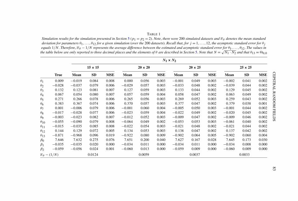
5. Simulation study. To demonstrate the effectiveness of our approach, weconducted a small simulation study using maximum likelihood estimation as out-lined in Sections 2 and 3. The model autocovariances were calculated accord-ing (2.5), with M = 1000 and p1 = p2 = 2. The exact parameter values for thesimulation were calibrated to the straw yield data analysis presented in the Sup-plement’s Appendix A. Grid sizes of (15×15), (20×20), (20×25) and (25×25)

were considered, where (20 × 25) constitutes the size grid in our real-data exam-ple.

For this simulation, we generated 200 Gaussian datasets with parameters θ =J� corresponding to quadrants I and II of the grid �,2 and β = (β0, β1, β2)

′; seeTable 1. In this case, β1 and β2 correspond to “row” and “column” effects, respec-tively, in the agricultural experiment considered. Here, the row and column effectsare obtained by regressing the vectorized response on the corresponding row andcolumn indices (since rows and columns are equally spaced). The X matrix usedin this simulation consisted of a column of ones followed by columns associatedwith the row and column effects and was taken from the analysis presented in theSupplement’s Appendix A. Given θ and β , we simulate directly from the corre-sponding multivariate Gaussian distribution. However, in cases where the grid sizeis extremely large, another potential approach to simulation would be circular em-bedding (Chan and Wood [9], Wood and Chan [44]), though it would be necessaryto properly account for any regression effects. The log Gaussian likelihood (up toconstants) given by (3.3) was numerically maximized for each simulated datasetusing the optim function in R (R Development Core Team [34]).

As demonstrated in Table 1, through an assessment of mean square error (mse),the model parameters can be estimated with a high degree of precision. Addition-ally, Table 1 illustrates that our asymptotic theory agrees with the finite sampleestimates for different grid sizes. Specifically, we provide the difference between

2That is, θ = [�−2,2,�−2,1,�−1,2,�−1,1,�0,2,�0,1,�1,2,�1,1,�2,2,�2,1,�−2,0,�−1,0,

�0,0]′ = (θ1, θ2, . . . , θ13)′.

CE

PSTR

AL

RA

ND

OM

FIEL

DS

83

TABLE 1Simulation results for the simulation presented in Section 5 (p1 = p2 = 2). Note, there were 200 simulated datasets and σθ denotes the mean standarddeviation for parameters θ1, . . . , θ12 for a given simulation (over the 200 datasets). Recall that, for j = 1, . . . ,12, the asymptotic standard error for θj

equals 1/N . Therefore, σθ − 1/N represents the average difference between the estimated and asymptotic standard error for θ1, . . . , θ12. The values inthe table below are only reported to three decimal places and the elements of θ are described in Section 5. Note that N = √

N1 · N2 and that θ13 = �0,0

N1 × N2

15 × 15 20 × 20 20 × 25 25 × 25

True Mean SD MSE Mean SD MSE Mean SD MSE Mean SD MSE

θ1 0.009 −0.019 0.084 0.008 0.000 0.056 0.003 −0.001 0.049 0.003 −0.002 0.041 0.002θ2 −0.028 −0.037 0.079 0.006 −0.029 0.057 0.003 −0.033 0.048 0.002 −0.039 0.044 0.002θ3 0.132 0.123 0.081 0.007 0.127 0.059 0.003 0.133 0.044 0.002 0.129 0.045 0.002θ4 0.067 0.054 0.080 0.007 0.057 0.059 0.004 0.058 0.047 0.002 0.063 0.049 0.002θ5 0.271 0.266 0.078 0.006 0.265 0.056 0.003 0.269 0.052 0.003 0.259 0.043 0.002θ6 0.383 0.367 0.074 0.006 0.370 0.057 0.003 0.377 0.047 0.002 0.379 0.038 0.001θ7 0.001 −0.006 0.079 0.006 −0.001 0.060 0.004 −0.005 0.050 0.003 −0.001 0.044 0.002θ8 −0.017 −0.028 0.077 0.006 −0.023 0.059 0.004 −0.022 0.049 0.002 −0.020 0.045 0.002θ9 −0.003 −0.023 0.082 0.007 −0.012 0.052 0.003 −0.009 0.047 0.002 −0.009 0.046 0.002θ10 −0.055 −0.090 0.079 0.008 −0.064 0.049 0.002 −0.053 0.053 0.003 −0.061 0.040 0.002θ11 −0.015 −0.035 0.085 0.008 −0.022 0.054 0.003 −0.021 0.048 0.002 −0.021 0.044 0.002θ12 0.144 0.129 0.072 0.005 0.134 0.053 0.003 0.138 0.047 0.002 0.137 0.042 0.002θ13 −0.871 −0.968 0.096 0.019 −0.922 0.080 0.009 −0.902 0.064 0.005 −0.902 0.060 0.004β0 7.646 7.632 0.275 0.076 7.651 0.200 0.040 7.627 0.167 0.028 7.645 0.173 0.030β1 −0.035 −0.035 0.020 0.000 −0.034 0.011 0.000 −0.034 0.011 0.000 −0.034 0.008 0.000β2 −0.059 −0.056 0.024 0.001 −0.060 0.013 0.000 −0.059 0.009 0.000 −0.060 0.009 0.000

σθ − (1/N) 0.0124 0.0059 0.0037 0.0033

84 T. S. MCELROY AND S. H. HOLAN

the mean standard deviation (over all of the cepstral parameters, except �0,0) andthe asymptotic standard deviation. This simulation shows that, as the grid size in-creases, the difference between the estimated standard error and the asymptoticstandard error goes to zero on average. We also provide the mean, standard devia-tion and mse for the individual parameters, including the mean parameters β; thisdemonstrates the bias properties, as well as the fact that the mse goes to zero asthe grid size increases. Finally, the average p-value for the Shapiro–Wilks test ofnormality for each simulation grid size (over all of the cepstral parameters) wasgreater than 0.4, with only one parameter out of the thirteen cepstral parametersfrom each simulation not exhibiting normality. Hence, the estimated parametersconverge to their asymptotic distribution and, as expected, their precision increaseswith sample size.

6. Conclusion. The general modeling approach and asymptotic theory wepropose extends the spatial random field literature in several directions. By pro-viding recursive formulas for calculating autocovariances, from a given cepstralrandom field model, we have facilitated usage of these models in both Bayesianand likelihood settings. This is extremely notable as many models suffer from aconstrained parameter space, whereas the cepstral random field model imposes noconstraints on the parameter values. More specifically, the autocovariance matrixobtained from our approach is guaranteed to be positive definite.

In addition, we establish results on consistency and asymptotic normality for anexpanding domain. This provides a rigorous platform for conducting model selec-tion and statistical inference. The asymptotic results are proven generally and canbe viewed as an independent contribution to the random field literature, expand-ing on the results of Mardia and Marshall [24] and others, such as Guyon [18].The simulation results support the theory, and the methods are illustrated throughan application to straw yield data from an agricultural field experiment (Supple-ment’s Appendix A). In this setting, it is readily seen that our model is easily ableto characterize the underlying spatial dependence structure.

Acknowledgments. We thank an Associate Editor and two anonymous refer-ees for providing detailed comments that helped substantially improve this article.The authors would also like to thank Aaron Porter for his assistance with imple-mentation of the Moran’s I statistic. This article is released to inform interestedparties of research and to encourage discussion. The views expressed on statisticalissues are those of the authors and not necessarily those of the U.S. Census Bureau.See [27] for the supplementary material.

SUPPLEMENTARY MATERIAL

Supplement to asymptotic theory of cepstral random fields (DOI: 10.1214/13-AOS1180SUPP; .pdf). The supplement contains a description of further appli-cations of the cepstral model, analysis of straw yield data, as well as all proofs.

CEPSTRAL RANDOM FIELDS 85

REFERENCES

[1] BANDYOPADHYAY, S. and LAHIRI, S. N. (2009). Asymptotic properties of discrete Fouriertransforms for spatial data. Sankhya 71 221–259. MR2639292

[2] BANERJEE, S., CARLIN, B. P. and GELFAND, A. E. (2004). Hierarchical Modeling and Anal-ysis for Spatial Data 101. Chapman & Hall, Boca Raton, FL.

[3] BESAG, J. (1974). Spatial interaction and the statistical analysis of lattice systems. J. R. Stat.Soc. Ser. B Stat. Methodol. 36 192–236. MR0373208

[4] BESAG, J. and GREEN, P. J. (1993). Spatial statistics and Bayesian computation. J. R. Stat.Soc. Ser. B Stat. Methodol. 55 25–37. MR1210422

[5] BESAG, J. E. (1972). On the correlation structure of some two-dimensional stationary pro-cesses. Biometrika 59 43–48. MR0315775

[6] BLOOMFIELD, P. (1973). An exponential model for the spectrum of a scalar time series.Biometrika 60 217–226. MR0323048

[7] BOCHNER, S. (1955). Harmonic Analysis and the Theory of Probability. Univ. CaliforniaPress, Berkeley. MR0072370

[8] BRILLINGER, D. R. (2001). Time Series: Data Analysis and Theory. Classics in Applied Math-ematics 36. SIAM, Philadelphia, PA. MR1853554

[9] CHAN, G. and WOOD, A. T. A. (1999). Simulation of stationary Gaussian vector fields. Statist.Comput. 9 265–268.

[10] CLIFF, A. D. and ORD, J. K. (1981). Spatial Processes: Models & Applications. Pion, London.MR0632256

[11] CRESSIE, N. and WIKLE, C. K. (2011). Statistics for Spatio-Temporal Data. Wiley, Hoboken,NJ. MR2848400

[12] CRESSIE, N. A. C. (1993). Statistics for Spatial Data. Wiley, New York. MR1239641[13] DAHLHAUS, R. and KÜNSCH, H. (1987). Edge effects and efficient parameter estimation for

stationary random fields. Biometrika 74 877–882. MR0919857[14] FUENTES, M. (2002). Spectral methods for nonstationary spatial processes. Biometrika 89

197–210. MR1888368[15] FUENTES, M., GUTTORP, P. and SAMPSON, P. D. (2007). Using transforms to analyze space–

time processes. In Statistical Methods for Spatio-Temporal Systems 77–150.[16] FUENTES, M. and REICH, B. (2010). Spectral domain. In Handbook of Spatial Statistics

(A. Gelfand, P. Diggle, M. Fuentes and P. Guttorp, eds.) 57–77. CRC Press, Boca Ra-ton, FL. MR2730949

[17] GEWEKE, J. (2005). Contemporary Bayesian Econometrics and Statistics. Wiley, Hoboken,NJ. MR2166278

[18] GUYON, X. (1982). Parameter estimation for a stationary process on a d-dimensional lattice.Biometrika 69 95–105. MR0655674

[19] HURVICH, C. M. (2002). Multistep forecasting of long memory series using fractional expo-nential models. International Journal of Forecasting 18 167–179.

[20] KEDEM, B. and FOKIANOS, K. (2002). Regression Models for Time Series Analysis. Wiley,Hoboken, NJ. MR1933755

[21] KIZILKAYA, A. (2007). On the parameter estimation of 2-D moving average random fields.IEEE Transactions on Circuits and Systems II: Express Briefs 54 989–993.

[22] KIZILKAYA, A. and KAYRAN, A. H. (2005). ARMA-cepstrum recursion algorithm for the es-timation of the MA parameters of 2-D ARMA models. Multidimens. Syst. Signal Process.16 397–415. MR2186185

[23] LI, H., CALDER, C. A. and CRESSIE, N. (2007). Beyond Moran’s I: Testing for spatial de-pendence based on the spatial autoregressive model. Geographical Analysis 39 357–375.

[24] MARDIA, K. V. and MARSHALL, R. J. (1984). Maximum likelihood estimation of models forresidual covariance in spatial regression. Biometrika 71 135–146. MR0738334

86 T. S. MCELROY AND S. H. HOLAN

[25] MCELROY, T. and HOLAN, S. (2009). A local spectral approach for assessing time seriesmodel misspecification. J. Multivariate Anal. 100 604–621. MR2478185

[26] MCELROY, T. S. and FINDLEY, D. F. (2010). Selection between models through multi-step-ahead forecasting. J. Statist. Plann. Inference 140 3655–3675. MR2674155

[27] MCELROY, T. S. and HOLAN, S. H. (2014). Supplement to “Asymptotic theory of cepstralrandom fields.” DOI:10.1214/13-AOS1180SUPP.

[28] MORAN, P. A. P. (1950). Notes on continuous stochastic phenomena. Biometrika 37 17–23.MR0035933

[29] NOH, J. and SOLO, V. (2007). A true spatio-temporal test statistic for activation detection infMRI by parametric cepstrum. In IEEE International Conference on Acoustics, Speechand Signal Processing, 2007. ICASSP 2007. 1 I–321. IEEE, Honolulu, HI.

[30] PIERCE, D. A. (1971). Least squares estimation in the regression model with autoregressive-moving average errors. Biometrika 58 299–312. MR0329169

[31] POLITIS, D. N. and ROMANO, J. P. (1995). Bias-corrected nonparametric spectral estimation.J. Time Series Anal. 16 67–103. MR1323618

[32] POLITIS, D. N. and ROMANO, J. P. (1996). On flat-top kernel spectral density estimators forhomogeneous random fields. J. Statist. Plann. Inference 51 41–53. MR1394143

[33] POURAHMADI, M. (1984). Taylor expansion of exp(∑∞

k=0 akzk) and some applications. Amer.

Math. Monthly 91 303–307. MR0740245[34] R DEVELOPMENT CORE TEAM (2012). R: A Language and Environment for Statistical Com-

puting. R foundation for statistical computing, Vienna, Austria.[35] ROSENBLATT, M. (1985). Stationary Sequences and Random Fields. Birkhäuser, Boston, MA.

MR0885090[36] ROSENBLATT, M. (2000). Gaussian and Non-Gaussian Linear Time Series and Random

Fields. Springer, New York. MR1742357[37] RUE, H. and HELD, L. (2010). Discrete spatial variation. In Handbook of Spatial Statistics

(A. Gelfand, P. Diggle, M. Fuentes and P. Guttorp, eds.). Chapman & Hall, London.[38] SANDGREN, N. and STOICA, P. (2006). On nonparametric estimation of 2-D smooth spectra.

IEEE Signal Processing Letters 13 632–635.[39] SOLO, V. (1986). Modeling of two-dimensional random fields by parametric cepstrum. IEEE

Trans. Inform. Theory 32 743–750.[40] STEIN, M. L. (1999). Interpolation of Spatial Data: Some Theory for Kriging. Springer, New

York. MR1697409[41] TANIGUCHI, M. and KAKIZAWA, Y. (2000). Asymptotic Theory of Statistical Inference for

Time Series. Springer, New York. MR1785484[42] TONELLATO, S. F. (2007). Random field priors for spectral density functions. J. Statist. Plann.

Inference 137 3164–3176. MR2365119[43] WHITTLE, P. (1954). On stationary processes in the plane. Biometrika 41 434–449.

MR0067450[44] WOOD, A. T. A. and CHAN, G. (1994). Simulation of stationary Gaussian processes in [0,1]d .

J. Comput. Graph. Statist. 3 409–432. MR1323050

CENTER FOR STATISTICAL RESEARCH AND METHODOLOGY

U.S. CENSUS BUREAU

4600 SILVER HILL ROAD

WASHINGTON, D.C. 20233-9100USAE-MAIL: tucker.s.mcelroy@census.gov

DEPARTMENT OF STATISTICS

UNIVERSITY OF MISSOURI

146 MIDDLEBUSH HALL

COLUMBIA, MISSOURI 65211-6100USAE-MAIL: holans@missouri.edu