Asymmetry in State Grant Distribution: WhyProximity to the State Capital Matters

JONATHAN R. CERVAS∗

University of California Irvinejcervas@uci.edu

March 21, 2016

Abstract

New Federalism and its subsequent policies have led to an increase in the size andamount of grants the federal government gives to the states. These grants have littleif any strings attached to them. Because legislators and bureaucrats have differentincentives, policy outcomes sought by either set of actors often contradict each other.This paper shows that the distribution of grants is asymmetric to the populations of thecounties in the state, with a disproportionate amount staying in the counties nearestthe state capitol.

Prepared for the 2016 Western Political Science Conference, San Diego, CA. March 2016.

∗The author would like to thank Ami Glazer, Maneesh Arora, and other members of Public Choice IIIat UCI for their valuable input on the paper. He also would like to thank Christopher Gagne for help withediting.

1

1 Introduction

The increased power of the states to allocate funds has coincided with a decline in leg-

islative power. The states are given increased power to distribute money to local areas yet

have less capacity to carry out the tasks. A vacuum is thus created. A full time executive

and their subsequent bureaucratic “fourth branch” are then tasked with bridging the gap

left. This paper looks at one implication of the shift of power from the legislature to the

bureaucracy. I present findings that show that counties that are adjacent geographically to

the state capital receive asymmetrical shares of the grants compared to the less proximate

counties.

In this paper I present a model which sets up a theoretical explanation for how federal

grants might be distributed asymmetrically based on proximity to the state capital. All

things being equal, a uniform and symmetrical distribution occurs when counties receive an

equal share of the funds as a function of their population. In cases where funds are not

distributed under this expectation, controlling for other mediating factors, citizens should

be concerned that their tax-money is being allocated in ways not consistent with democratic

practice.

The allocation and redistribution of taxes has been central to much of the political debate

in American history. In the federalist papers, the founders debated how much governmental

power should be allocated to the central government. Federalist, who favored a strong central

government, were forced to compromise and ratify the tenth amendment, giving states more

influence then they otherwise would have preferred. The Civil War, and eventually World

War II, led to an increasingly stronger central government, with power mostly increasing in

the executive branch. While James Madison wrote that the legislature is where the people’s

voice would be the loudest, it has become clear that executive authority at both the federal

and state level has captured an immense amount of power.

2

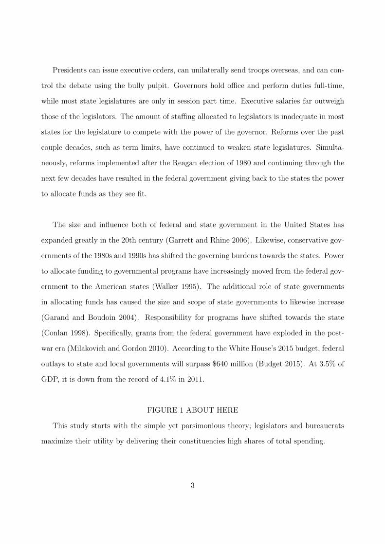
Presidents can issue executive orders, can unilaterally send troops overseas, and can con-

trol the debate using the bully pulpit. Governors hold office and perform duties full-time,

while most state legislatures are only in session part time. Executive salaries far outweigh

those of the legislators. The amount of staffing allocated to legislators is inadequate in most

states for the legislature to compete with the power of the governor. Reforms over the past

couple decades, such as term limits, have continued to weaken state legislatures. Simulta-

neously, reforms implemented after the Reagan election of 1980 and continuing through the

next few decades have resulted in the federal government giving back to the states the power

to allocate funds as they see fit.

The size and influence both of federal and state government in the United States has

expanded greatly in the 20th century (Garrett and Rhine 2006). Likewise, conservative gov-

ernments of the 1980s and 1990s has shifted the governing burdens towards the states. Power

to allocate funding to governmental programs have increasingly moved from the federal gov-

ernment to the American states (Walker 1995). The additional role of state governments

in allocating funds has caused the size and scope of state governments to likewise increase

(Garand and Boudoin 2004). Responsibility for programs have shifted towards the state

(Conlan 1998). Specifically, grants from the federal government have exploded in the post-

war era (Milakovich and Gordon 2010). According to the White House’s 2015 budget, federal

outlays to state and local governments will surpass $640 million (Budget 2015). At 3.5% of

GDP, it is down from the record of 4.1% in 2011.

FIGURE 1 ABOUT HERE

This study starts with the simple yet parsimonious theory; legislators and bureaucrats

maximize their utility by delivering their constituencies high shares of total spending.

3

2 Literature Review

Niskanen’s (1971) theory of bureaucracy shows how a bureaucrat can influence the size

of their agencies budgets. In addition to other incentives, they seek to maximize their own

personal welfare. Often these benefits include the desire for prestige, influence, and high

salaries. This can lead to budgets that exceed what is required to meet the demands of the

population. The public is rationally ignorant (Downs 1957), and that leads citizens to have

limited abilities to monitor public employees (Mueller 2003).

The capacity of state legislatures varies greatly among the many states. The amount of

time the legislature meets is written in state law. The capacity of a legislature is closely

related to the level of professionalism the body holds (Squire 2007). Functionally speaking,

state legislatures are institutionally similar to the US Congress. They differ in terms of the

amount of influence on public policy they have. The capacity for the legislature to control

the actions of the bureaucracy is affected by the resources available to them (Bawn 1995).

The bureaucracy’s ability to influence lawmaking is systematically different across the many

states (Barrilleaux 1999). States that have highly institutionalized legislatures are less likely

to delegate policy authority to the governor then those states with less institutionalized

legislatures (Huber and Shipan 2002). Despite efforts to professionalize state legislatures

(King 2000), Boushey and McGrath (2015) show that the executive/legislative imbalance of

power has increased over time. Policies enacted to supposedly ”reign in” politicians such as

term limits often have the opposite affect than there intended goal. Term limits have been

shown to weaken the legislature vis a vis other branches (Baker and Hedge 2013). These

populous reforms instead may have led to weaken institutional power for legislatures and

coincidentally strengthened unelected bureaucrats (Volden 2002, Rosenthal 2009).

Institutionalization of state legislatures is often measured using a professionalization in-

dex (Squire 2007). Professionalization has been measured empirically as a function of the

amount of time the legislature spends in session, the size of the staff provided to a legislator,

4

and the amount of compensation. The size of the staff and resources available to a legisla-

tor is of particular importance when dealing with issues of spending. The scarce time and

resources available to a legislator to devote to ensuring high funding levels to their district.

Career politicians have incentives to generate benefits for their constituents; staff can help

subsidize the opportunity costs of securing funds (Grossbeck and Peterson 2004). Woods

and Baranowski (2006) show that careerism reduces legislative influence on the bureaucracy,

while resources help to increase it. In a similar vein, professionalism can entice legislators

to increase funding to their constituents in order to enhance their career objectives while

providing them the resources to do so (Woods and Baranowski 2006, Krause and Woods

2014). Term limits can also work in concert with professionalism of the state legislature to

move power from the legislative to the executive branch. Institutional knowledge, expertise,

and continuity is lost as term limits increase the turnover (Squire 2007).

The literature on political control through agency design has resulted in mixed findings

about whether the legislature uses design as a tactic to maintain influence over the bureau-

cracy (Reenock and Poggione 2004, Potoski 1999). Bureaucratic capture of power thus exists

where legislative bodies are weak, unprofessional, or understaffed. When this happens, indi-

vidual legislators lose the ability to influence how funds are distributed. This results in power

shifting from the legislature to the bureaucracy, and ostensibly, to the Governor. Because

both the Governor and members of the bureaucracy respond to their own preferences, their

incentive is to allocate funds to places that maximize their benefit.

FIGURE 2 ABOUT HERE

The state capital houses the bureaucracy’s central functions. The absence of a legisla-

ture would mean that the bureaucratic powers, which reside in the capital, would have full

power to distribute state funds to local governments and award grants to those areas. A

bureaucracy that is unaccountable to the public or a legislative body would have no incen-

tive to distribute funds anywhere where they would not benefit. The geographic diversity

5

of members of the legislature restricts their ability to do so, ensuring funds follow a more

equitable distribution. To be sure, some literature has demonstrated that political influence

can affect the amount of funds that a county attracts. Using court-ordered redistricting as

a natural experiment, Ansolabehere et al (2002) found that federal funds flowed at higher

rates to counties that had greater representation in the US House of Representatives before

redistricting. Additionally, a large literature suggests that spending by neighboring states

increases spending in a state (Case et al 1993, Boarnet and Glazer 2002). The relative power

of the legislature acts as a check on the bureaucracy. In the margins, however, it can be ex-

pected that the bureaucracy will can achieve their ends. That leads us to our first hypothesis:

H1: The relative share of state funds a county receives will be greater in the proximate

counties to a state capital than in more distant geographical locations.

State capitals themselves all have one important characteristic they share with each

other; they were all selected over a century ago. The location of the capital is an insti-

tutional choice, and the selection of a location might not be distinct from the distribution

of the population. In a recent article, Campante and Do (2014) demonstrate that isolated

state capitals are more prone to corruption and that they are associated with lower levels

of accountability. If in fact isolated state capitals are not held to account, evidence would

be found in the distribution of federal grants to the different counties. The theory is that

isolated state capitals are also isolated and distant from the public mind, and that without

attention by the media, which typically happens in local newspapers, they are more able to

accomplish goals that don’t reflect the preferences of the people. This leads to hypothesis

two:

H2: States with isolated state capitals will distribute grants more asymmetrically.

6

3 Empirical Strategy

Testing these propositions will rest upon the results of three tests. First, I will demon-

strate that proximity to the state capital affects the amount of federal funds a county re-

ceives. Second, I will show that isolated state capitals do a poor job at distributing grants

proportionate to the population. Lastly, I will use an instrument to demonstrate that the

state capital is in fact itself exogenous from theoretical world where states choose their state

capitals in order to distribute these grants in an asymmetric way.

In testing our theoretical propositions, I will look at federal grants that are distributed

by states. Federal grants often have few constraints from the federal government as to how

they must spend them. Often times the federal government allocates money in block grants.

This money holds little or no rules and are given to the states to distribute how they please.

I test whether these grants are spent evenly among the counties on a per capita basis. Grant

data from 2010 are used to test our propositions.

Data on grants is collected from the now-defunct Consolidated Federal Funds Report. In

this data, all federal transfers to states and counties are listed including retirement funds,

procurements, military and non-military salaries, and other direct transfers. I am only con-

cerned with grants, reasoning that they are the source of funds that bureaucrats can have

the most influence over how they are distributed around the state. Whereas retirement funds

will be concentrated in places where the population is older, military spending in places that

have bases, there is no a priori reason to believe that grants would be spent more in one place

than another on a per capita basis. The large amount of data allows us to systematically

determine the patterns of asymmetry in the distribution of these revenues.

County receipts from state funds are also generated from the Consolidated Federal Funds

Report.

To account for the wide variation in amount of funds counties receive I must measure

them as per-capita dollars. It is then necessary to create a dependent variable that relates

7

all counties across states, such that the share of per capita dollars divided by the share of

the state population. The resultant dependent variable is a ratio. The formula is as follows:

countysharei,t = ln((countyrevenuei,tstaterevenuei,t

)

(countypopulationi,t

statepopulationi,t))

where i is the county and t is the year. 1

As a county’s share of revenue increases significantly above its share of the population,

the ratio of the share of revenue and the share of the population can get quite large. For

counties that receive lots of state support but contain relatively few people, their scores can

reach upwards of 50. Likewise, this ratio is constrained to greater than 0 for all places. So,

while those that get significantly less than their share move slowly towards 0, those with

larger shares go up exponentially. This becomes especially problematic if a county has a

population close to zero, but gets any amount of funds, even if just a small percentage of

the whole. 2 I therefore take the natural log of this fraction to account for those counties

that exhibit this trend. I then reconstruct the dependent variable to range from 0 to 1 3 for

1A county that scores a one on this scale is one that receives funds that are equal to their per capitashare of the population. This measure unfortunately biases the estimates for those counties that receive ahigher proportion then their populations would otherwise dictate. For instance, if a county has 10% of thestate population and gets 10% of the revenue, they have a score of 1

ShareRevenue

SharePopulation=

0.10

0.10= 1

If they get less of a share than they should, say they are 10% of the population but get just 5% of therevenue, their score is

0.05

0.10= 0.5

On the other hand, if a county accounts for 10% of the population but get 20% of the revenue

0.2

0.1= 2

2

0.01

0.0001= 100

3A value of zero indicates the lowest ratio, 1 indicates the highest ratio.

8

easy interpretation. 4

4 Distance

Distance can conceptually mean multiple things. For instance, I can measure distance

from one point to another in some metric such as miles. This distance can be from the cen-

ter point of some legal boundary, from the closest point between two locations, the furthest

point between two, the largest population base in the unit, or some combination of these.

There are also scenarios where absolute distance matters less than ease of navigation. For

instance, maybe only whether two places are reachable via an automobile in some arbitrary

time is important. The presence or absence of an airport and the availability of flights be-

tween places could also provide some information about social distance.

For the purposes of this paper, distance is measured in miles between the centroid point

of a county and the center of the urban area of the capital. I chose this metric for two

reasons: 1, I believe theoretically that distance in absolute terms helps to differentiate the

counties from one another. Although a place that is six hours away via car and one that is

eight miles would likely not differ in any great respect for our purposes, I do believe that lo-

cations that are two hours are different than those that are six or eight. I have also selected

this metric for its convenience. Some counties don’t have large cities that could be used

as a central feature. Others may have multiple cities or sprawling metropolises. Counties

particularly on the east side of the Mississippi are small in square miles and have cities that

span multiple counties. By keeping our measures simple, I can still get at our theoretical

4As a robustness check, I will alternatively run a regression that only include counties with populationsgreater than 25,000. The median population for counties is right around 25,000 in 2010, while the meanpopulation is almost 100,000. While I lose half our observations, I also diminish the chances of biasedestimates. This only excludes a fragment of the observations, and there is no reason to believe those countiesexcluded are endogenous to the independent variable of distance. As it is, if every county received a perfectshare of the revenues, all values would be one. The theory presented in this paper suggests that countiesshould not be equal. Institutional incentives create geographical differences in county shares of revenue. Inan additional robust check, I will eliminate the bottom and top 5% of all counties by state and run theregression. This eliminates any possible outliers.

9

construct. I expect that the geographical distance will have diminishing returns. A place

that is 200 miles from the capital will have very little difference to a place 400 miles. For

this reason, distance will be modeled with a quadratic fit. Transforming the distance with a

natural log will enable linear estimation in the face of distances that could reach nearly 500

miles in some states.5 Additionally, distance will be rescaled so that the closest distance is

0 and the furthest distance is 1.6

Several controls are used to account for the vast differences between the counties and the

fact that counties exist within states that themselves differ in their size, density, and political

ideologies. The data on revenues and grants from states to counties is transformed for the

dependent variable and can be interpreted as the ratio of the grants the county receives in a

given year divided by its share of population the county has of the total state. Controlling

for the population of a county is necessary because I do not expect a large county such as

Los Angeles County to get the same percentage of funds as a small population county such

as Sierra County. Additionally, places that have national parks where urban development is

restricted a subject to the sort of large ratio explained in the previous sections. I account

for density of the population in the county, and in other models the density of the entire

state. There is reason to believe that density at both levels might affect the amount of

grants a county gets. A county that is rural might still have needs for services such as court

houses, police stations, or forest rangers. This would work to increase the share they get as

a proportion. On the other hand, the overall density of a state might affect the distribution

of grants. If only a small number of counties are rural, all the power in the bureaucracy and

legislature might come from urban interests and ignore their rural counterparts. Multiple

specifications of the model will include different configurations of density controls.

5Using Google Maps, any user can easily measure the distance between two points. Pennsylvania isapproximately 315 miles from the two furthest points. Texas is 800 miles between some points. Californiais 825 miles North to South.

6This is done for ease of interpretation and does not in any way affect the statistical results of the model.Both the independent and the dependent variable are coded 0 to 1.

10

FIGURE 3 ABOUT HERE

Further extension of the controls of geography need to account for counties that have

large geographical footprints. These counties might require a higher then average share of

revenue, especially if they contain expensive public goods such as interstate freeways. There

are good theoretical reasons to believe that population growth could either increase the funds

a county receives or reduces them.7 If a state had foresight to growth patterns, it might al-

locate more funds to support infrastructure projects and other spending that a stable area

might not need. On the other hand, expenditures where there is explosive growth might

have lagged behind as legislatures are not full time and can not continuously allocate those

funds. Other reasons include that places that have high growth will be under-represented in

the legislature until redistricting fixes any malapportionment problems.

I also control for median income.8 As with population size, there is not particular reason

to expect a dollar to go as far in Sierra County as it might in Los Angeles County. Controls

for how urban/rural a county is are also included. Rural counties are distinctly unique from

urban areas. Rural areas need less infrastructure and likely less need for government services

generally. Large tracts of land, especially in the west, are owned by the federal government.

There is no need for states to spend any of their federal grants in these areas. For this rea-

son, in addition to its massive size, I eliminate Alaska. Alaska is a geo-spatially large state

and has very few residents. It does have valuable natural resources, however, and in many

ways is different from other states. 9 For these reason, I need to account for it in our models.

TABLE 1 ABOUT HERE

Additional statistical controls are included to ensure our distance measure isn’t biased

in it’s coefficient. Regulation index indicates the amount of economic freedom a state has.

7I ran the regressions with actual growth percentage and the the coefficient was significant but did notaffect the other coefficients and only marginally affected the R-Squared

8In thousands of dollars.9Hawaii is also excluded from the analysis for unrelated reasons, mostly due to that lack of data.

11

Racial dissimilarity is the amount of racial dissimilarity in a state. 10 The share of total

employed in a state that are government employees, a dummy if the capital city is the largest

city in the state, and regional dummies round out the statistical controls.

The regression equation will follow the form:

countysharei,t = α + β1distancei

+ β2distancesqri

+ β3incomei,t

+ β4capitalcityi,t

+ β5densityi,t

+ β6sovshareofemployeesi,t

+ β7regulationindexi,t

+ β9racialdissimilarityi

+ β10regiondummiesi

+ β11rurali

+ ε

5 Discussion/Results

Our main explanatory variable that describes the differences between counties in terms

of proximity to the state capital is statistically significant in all years measured. The coef-

ficient is negative, indicating that counties close to the state capital receive a higher than

expected share of grants from the federal government, controlling for their population size

and growth. Even through multiple specifications of the model, Distance from the capital,

10How heterogeneity a state’s demographics are.

12

along with income, density, and percent rural are statistically significant at the .01 level.

The south regional dummy is also significant in these models, although the coefficient size is

not substantially large. These models control for state fixed effects and the standard errors

are robust to control of heteroskedasticity.

It should also be noted that the size of the grants and revenues also drastically increased

over this time, so differences in 1990 are less in constant dollars than in 2010. The construc-

tion of the dependent variable makes it difficult to interpret what sums of money is affected.

It appears to make more sense to consider the impact of a county that is as far as possible

away from the capital but also with a very large population. Take Clark County, NV for

instance, the 2010 revenues from the state were nearly $1.5 billion. Receiving one percent

less revenue would be $15 million. Clark County contains nearly three-quarters of the popu-

lation of Nevada, so other counties would benefit greatly from any tax money redistributed

from Clark County.

TABLE 2 ABOUT HERE

The second hypothesis this paper test is whether states that have isolated state capitals

do a poor job of equally distributing grants. These states with isolated capitals would os-

tensibly free the bureaucracy from the checks and balances of a well informed public. Places

that have part-time legislatures mean that newspapers don’t have full time bureau to cover

state government. This in turn might give bureaucrats more power to direct funds towards

projects they prefer. The dependent variable here is a gini score of inequality in the dis-

tribution of grants in 2010. The main independent variable of interest is Average Logged

Distance of a state. This measure is adopted from Campante and Do (2010), and it reflects

how much a state’s population is centered spatially around the state capital. This measure

maintains monotonicity; in a state where the population is completely in the state capital

the measure will be 0. When the entire population lives the furthest possible distance from

13

the capital, the state will have a 1 on the index. The intuition is actually quite simple: “spa-

tial proximity to power increases political influence” (Ades and Glaeser 1995). A number of

specifications will be reported to show the consistent strength of average logged distance as

a predictor of how a state distributes funds.

FIGURE 4 ABOUT HERE

TABLE 3 ABOUT HERE

In all the different specifications of the model, the Average logged distance variable re-

mains significant. This gives us more evidence that isolated state capitals do a poor job of

equally distributing grants. This has the additional feature of further enhancing our con-

fidence that distance might play a factor in how money is distributed. States that have

populations that are more centered on the seat of government can more easily maintain a

check on the power of bureaucrats. The percent of the state that is in urban areas is also

highly significant and positive. This suggests that as a state becomes more urban, they have

a harder time equally dividing grants. The concentration measure, however, is the single

largest predictor of how in-equal a state is in distributing grants.

TABLE 5 ABOUT HERE

6 Instrument Verification

Endogeneity is always a problem social scientists must worry about. While I find it hard

to believe that the distribution of grants can affect where the location of the state capital

is, there is still a possibility that this is the case. To test that another source of county

funds isn’t subject to the same effect of proximate, I substitute the dependent variable for

a source of revenue that is fixed by law. In this test, we use the county share of retirement

and disability. While it is technically feasible that people who collect these funds choose to

14

live very close in proximity to the state capital, there is not prima facia reason to think that

patterns of geography related to state capital affect where people retire.

TABLE 6 ABOUT HERE

In fact it appears that, unlike federal grants, retirement and disability spending is unre-

lated to proximity to the state capital. This further enhances our already strong inclination

to believe that bureaucrats can, at least in the margins, steer federal grants towards the

areas they live in.

7 Conclusion

There are many valid reasons why there might be variation in allocation of taxpayer

funds. Among the ones that seem most appropriate is where there is most need, perhaps

for infrastructure, to spur economic growth, or to relieve poverty. Not among the reasons

acceptable to democratic theorist are things outside the citizenry’s ability to control such as

geographic proximity to the state capital or bureaucratic capture of power from the elected

body. The results from this paper indicate that there is an asymmetry between areas driv-

able from the capital and those further away in regards to grants. For the other years where

I measure all revenues from the state, the coefficients are insignificant. The geographic

locations of a state capitals are unlikely to change and most have been stable for most of

American history. These locations were chosen long before shifting populations and explosive

growth increased populations across the US. State capitals all differ in their characteristics

such as demographics, size, and proximity to major cities (some are the largest in their

state, such as Boston, Phoenix, and Denver, while others are small and rural like Carson

City and Montpelier). They all hold one thing consistent, and that is that they house the

state bureaucratic apparatus, which has increasingly become vested with power to distribute

taxpayer money. The findings in this paper represent some evidence that legislative power

15

can be dominated by an increasingly strong bureaucracy. The results do not make claim that

some mechanism specifically has driven this trend, just that there seems to exist some power

imbalances that result in an asymmetric distribution of federal grants. If these results hold

in other circumstances, the public should be concerned with its ability to check government

through regular elections.

8 Bibliography

Ades, Alberto F. and Edward L. Glaeser. 1995. “Trade and Circuses: Explaining UrbanGiants,” Quarterly Journal of Economics 110: 195-227.

Albouy, David. 2013. ”Partisan Representation in Congress and the Geographic Distri-bution of Federal Funds.” The Review of Economics and Statistics 95(1): 127–141.

Ansolabehere, Stephen, Alan Gerber, Jim Snyder. 2002. ”Equal Votes, Equal Money:Court-Ordered Redistricting and Public Expenditures in the American States”. AmericanPolitical Science Review 94(4): 757-777.

Ansolabehere, Stephen, and James M. Snyder Jr. ”Party Control of State Governmentand the Distribution of Public Expenditures.” Scandinavian Journal of Economics 108(4):547-569.

Baker, Travis J., and David M. Hedge. 2013. “Term Limits and Legislative-ExecutiveConflict in the American States.” Legislative Studies Quarterly 38:237–58.

Bawn, Kathleen. 1995. ”Political Control Versus Expertise: Congressional Choices aboutAdministrative Procedure.” American Political Science Review 89(1): 62-73.

Boarnet, Marlon G., and Amihai Glazer. 2002. ”Federal Grants and Yardstick Compe-tition.” Journal of Urban Economic 52: 53-64.

Boushey, Graeme T., and Robert J. McGrath. Forthcoming. ”Experts, Amateurs, andthe Politics of Delegation in the American States.”

Campante, Filipe R. and Quoc-Anh Do. 2010. “A Centered Index of Spatial Concen-tration: Expected Influence Approach and Application to Population and Capital Cities.”Harvard Kennedy School (unpublished).

Campante, Filipe R., and Quoc-Anh Do. 2014. Isolated Capital Cities, Accountabilityand Corruption: Evidence from US States. American Economic Review 104(8): 2456-81.

16

Downs, Anthony, ”An Economic Theory of Democracy.” New York: Harper & Row. 1957.

Garrett, Thomas A., and Russell M. Rhine. 2006. ”On the Size and Growth of Govern-ment.” The Federal Reserve Bank of St. Louis Review.

Grossback, Lawrence J., and David A.M. Peterson. 2004. ”Understanding InstitutionalChange: Legislative Staff Development and the State Policymaking Environment.” Ameri-can Politics Research 32(1): 26-51.

Kelly, Nathan J., and Christopher Witko. 2012. ”Federalism and American Inequality.”Journal of Politics 74(2): 414-426.

King, James D. 2000. ”Changes in Professionalism in U.S. State Legislatures.” Legisla-tive Studies Quarterly 25(2): 327-343.

Krause, George A., and Neal D. Woods. 2014. ”State Bureaucracy: Policy Delegation,Comparative Institutional Capacity, and Administrative Politics in the American States.” inThe Oxford Handbook of State and Local Government, edited by Donald P. Haider-Markel.

Lee, Frances E. 1998. ”Representation and Public Policy: The Consequences of SenateApportionment for the Geographic Distribution of Federal Funds.” Journal of Politics 60(1):34-62.

Lee, Frances E. 2000. ”Senate Representation and Coalition Building in DistributivePolitics.” American Political Science Review 94(1): 59-72.

Martin, Paul S. 2003. ”Voting’s Rewards: Voter Turnout, Attenative Publics, and Con-gressional Allocation of Federal Money.” American Journal of Political Science 47(1): 110-127.

Mueller, Dennis C. 2003. ”Public Choice III.” New York: Cambridge University Press.

Musgrave, Richard A. 1997. ”Devolution, Grants, and Fiscal Competition.” Journal ofEconomic Perspectives 11(4): 65-72.

Niskanen, William. Bureaucracy and Representative Government. Chicago: Aldine-Atherton, 1971.

Potoski, Matthew. 1999. ”Managing Uncertainty through Bureaucratic Design: Admin-istrative Procedures and State Air Pollution Control Agencies.” Journal of Public Adminis-tration Research and Theory 9(4): 623-639.

Reenock, Christopher and Sarah Poggione. 2004. “Bureaucratic Control by Design: Ex-plaining State Legislators Willingness to Use Ex Ante Tactics in Air Pollution Control.”

17

Legislative Studies Quarterly 29(August): 393-406.

Rich, Michael J. 1989. ”Distributive Politics and the Allocation of Federal Grants.”American Political Science Review 83(1): 193-213.

Rosenthal, Alan. 2009. Engines of Democracy: Politics and Policymaking in State Leg-islatures. Washington, DC: CQ Press.

Rodden, Jonathan. 2010. “The Geographic Distribution of Political Preferences.” An-nual Review of Political Science, 13: 321-340.

Squire, Peverill. 2007. “Measuring State Legislative Professionalism: The Squire IndexRevisited.” State Politics and Policy Quarterly 7(June): 211-227.

Uppal, Yogesh, and Amiahi Glazer. 2015. ”Legislative Turnover, Fiscal Policy, and Eco-nomic Growth: Evidence from U.S. State Legislatures.” Economic Inquriy 53(1): 91-107.

Volden, Craig. 2002. “Delegating Power to Bureaucracies: Evidence from the States.”Journal of Law, Economics, & Organization 18(1):187–220.

Walker, David B. 1995. The Rebirth of Federalism: Slouching Toward Washington.Chatham, NJ: Chatham House.

Woods, Neal D., and Michael Baranowski. 2006. ”Legislative Professionalism and In-fluence on State Agencies: The Effects of Resources and Careerism.” Legislative StudiesQuarterly 31(4): 585-609.

United States Printing Office. 2015. ”Fiscal Year 2015, Historical Tables: Budget of theU.S. Government.”

18

Figure 1: Federal Outlays to State and Local Governments: 1940 - 2019

19

Figure 2: Theoretical Distribution of Power over Government

20

Table 1: Descriptive Statistics

Variable mean sd min max

Grants (in 1000s) 153,771 873,018 0 34,530,000Income (median) 426.5 110.7 188.6 1,142

Distance (10s Miles) 119.2 77.30 0.778 506.1Professionalization Score 0.185 0.109 0.0270 0.626

Density 142.2 148.6 6 1,210Regulation Index 6.065 0.486 5.047 7.377

Racial dissimilarity 0.262 0.132 0.0251 0.473North East 0.0672 0.250 0 1

Midwest 0.344 0.475 0 1South 0.457 0.498 0 1West 0.132 0.339 0 1

Regional Dummy variables can be read as percentage of counties inthat region.

21

Figure 3: 2010 Share of Revenues by Share of Population

22

Table 2: Robust Weighted Least Squares Regression, County Share of Federal Grants

VARIABLES (1) (2) (3) (4) (5) (6)

Distance -0.269* -0.341** -0.271* -0.335** -0.323** -0.335**[0.130] [0.124] [0.129] [0.096] [0.118] [0.096]

Distance Squared 0.257* 0.235* 0.158 0.206* 0.195 0.206*[0.104] [0.089] [0.105] [0.080] [0.100] [0.080]

Median Income -0.000*** -0.002*** -0.002*** -0.002*** -0.002***[0.000] [0.000] [0.000] [0.000] [0.000]

Median Income Squared 0.000*** 0.000*** 0.000*** 0.000***[0.000] [0.000] [0.000] [0.000]

Capital Largest City -0.025 -0.023* -0.025* -0.027** -0.025*[0.013] [0.010] [0.011] [0.009] [0.011]

Density 0.015* 0.026*** 0.023*** 0.026*** 0.023***[0.008] [0.006] [0.005] [0.004] [0.005]

Gov. Share Employees 1.347** 1.051* 1.126*** 1.051*[0.434] [0.426] [0.266] [0.426]

Regulation Index 0.020 0.027* 0.026** 0.027*[0.014] [0.013] [0.009] [0.013]

Racial dissimilarity -0.162 -0.072 -0.090 -0.072[0.087] [0.075] [0.054] [0.075]

South Dummy -0.078*** -0.096*** -0.101*** -0.096***[0.019] [0.015] [0.013] [0.015]

Northeast Dummy -0.019 -0.022 -0.027 -0.022[0.021] [0.020] [0.017] [0.020]

Midwest Dummy -0.041* -0.054** -0.058** -0.054**[0.020] [0.019] [0.018] [0.019]

County Percent Rural -0.000*** -0.000* -0.000***[0.000] [0.000] [0.000]

Observations 3,034 3,034 3,034 3,034 1,534 3,034R-squared 0.019 0.229 0.412 0.425 0.428 0.425State FE YES YES YES YES YES YES

Robust standard errors in brackets*** p<0.001, ** p<0.01, * p<0.05

Models 1-4 are all counties. Model 5 is only those with populations over 25,000. Model 6doesn’t include any county that is smaller than 5 percentile or larger than the 95 percentile(Trimmed Model) State Urban Percent not reported

23

Table 3: Gini Index of Equality of Dispersion of Federal Grants

State Gini Index State Gini Index State Gini Index

RI 0.2347 ID 0.3139 PA 0.3891IA 0.2682 NC 0.3181 WY 0.3905TN 0.2688 AL 0.3185 AZ 0.3954OR 0.2708 MI 0.3196 KY 0.4073CT 0.2735 KS 0.3233 MO 0.4287MS 0.2742 NM 0.3281 VA 0.4326DE 0.2792 AR 0.3281 IL 0.4460SC 0.2851 NE 0.3348 MD 0.4565IN 0.2883 LA 0.3359 CO 0.4565

WV 0.2933 NH 0.3378 NJ 0.4692CA 0.2964 GA 0.3454 UT 0.4696WI 0.3022 TX 0.3470 FL 0.4958ME 0.3044 VT 0.3506 MT 0.5000MN 0.3080 NY 0.3587 SD 0.5212OK 0.3090 WA 0.3725 ND 0.5661OH 0.3110 MA 0.3850 NV 0.5983

Gini scores calculated for each state. Inequality measured as percent ofgrants divided by percent of population, by county. High scores indicateasymmetric distribution of funds.

24

Table 4: Descriptive Statistics for Gini Index Regressions

VARIABLES mean sd min max

Gini Index 0.362 0.082 0.235 0.598Average Logged Distance 0.670 0.122 0.437 0.876Median Income 50864 9764 32685 68385Regulation Index 6.289 0.581 5.047 7.377Racial dissimilarity 0.273 0.121 0.025 0.473Share of value added in mining 0.021 0.059 0.000 0.718State Area (Logged) 10.286 1.409 6.952 12.475Maximum Distance State (Logged) 5.635 0.816 3.756 6.715Population (Logged) 15.396 1.042 13.016 17.104Income (Logged) 9.536 0.136 9.143 9.760State Percent Urban 0.729 0.143 0.264 0.890Legislature Professionalism 0.259 0.160 0.027 0.626Gov. Share of Total Employees 0.156 0.025 0.124 0.238Percent of Population in State Capital 0.076 0.114 0.004 0.466Capital Largest City (dummt) 0.286 0.457 0.000 1.000

25

Figure 4: Gini Index Score and Average Log Distance by State

26

Table 5: OLS Regression, Gini Index Score for Inequality in Distribution of Federal Grants to counties by State

VARIABLES (1) (2) (3) (4)

Average Logged Distance 0.3630 0.4517* 0.4268* 0.6140**[0.184] [0.196] [0.209] [0.213]

State Area (Logged) 0.0107 0.0123 0.0346 0.0381[0.027] [0.028] [0.036] [0.038]

Maximum Distance State (Logged) -0.0247 -0.0146 -0.0058 -0.0250[0.048] [0.045] [0.050] [0.053]

Income (Logged) 0.1494 0.0717 0.1746[0.152] [0.217] [0.212]

Population (Logged) -0.0267 -0.0611** -0.0280[0.014] [0.021] [0.027]

Proportion of Population with College Degree 0.6164 0.5822 0.1185[0.673] [0.854] [0.848]

Government Share of Total Employeed 0.2225 1.1711[0.632] [0.730]

State Percent Urban 0.2883* 0.3818**[0.136] [0.133]

Racial dissimilarity -0.3282[0.170]

Regulation Index -0.0464*[0.022]

Share of value added in mining -0.1863[0.112]

Legislature Professionalism -0.1692[0.155]

Regional Dummies X XObservations 48 48 48 48R-squared 0.145 0.327 0.427 0.572

Standard errors in brackets*** p<0.001, ** p<0.01, * p<0.05

27

Table 6: (Instrument) County Share of Retirement and Disability

VARIABLES (1) (2) (3) (4)

Distance 0.241 0.150 0.173 0.107[0.151] [0.125] [0.092] [0.070]

Distance Squared -0.176 -0.123 -0.116 -0.062[0.131] [0.111] [0.070] [0.061]

Median Income -0.000* -0.000* -0.000[0.000] [0.000] [0.000]

Median Income Squared 0.000 0.000[0.000] [0.000]

Capital Largest City -0.011 -0.015 -0.018[0.010] [0.011] [0.010]

Density -0.010*** -0.008*** -0.008***[0.003] [0.001] [0.002]

State Percent Urban 0.195**[0.056]

Government Share Employees 0.253 -0.056[0.362] [0.423]

Regulation Index -0.032** -0.017*[0.010] [0.008]

Racial dissimilarity -0.213** -0.095[0.064] [0.054]

South Dummy 0.061*** 0.034*[0.016] [0.015]

Northeast Dummy -0.005 -0.010[0.018] [0.019]

Midwest Dummy 0.013 0.002[0.014] [0.015]

County Percent Rural -0.000[0.000]

Observations 3,037 3,034 3,034 3,034R-squared 0.018 0.229 0.424 0.351State FE YES YES YES YES

Robust standard errors in brackets*** p<0.001, ** p<0.01, * p<0.05

28