Asymmetric Grading Error and Adverse Selection:...

Journal ofAgricultural and Resource Economics 24(1):57-79Copyright 1999 Western Agricultural Economics Association

Asymmetric Grading Error andAdverse Selection: Lemons in the

California Prune Industry

James A. Chalfant, Jennifer S. James,Nathalie Lavoie, and Richard J. Sexton

Grading systems are often introduced to address the classic adverse selectionproblem associated with asymmetric information about product quality. However,grades are rarely measured perfectly, and adverse selection outcomes may persistdue to grading error. We study the effects of errors in grading, focusing onasymmetric grading errors-namely when low-quality product can erroneously beclassified as high quality, but not vice versa. In a conceptual model, we show theeffects of asymmetric grading errors on returns to producers. Application to theCalifornia prune industry shows that grading errors reduce incentives to producemore valuable, larger prunes.

Key words: adverse selection, grading errors, product quality, prunes

Introduction

Adverse selection is a concern in many agricultural product markets due to imperfectinformation about product quality. Grading is one way to mitigate this problem. Theprice premiums and discounts associated with commodity grades provide incentivesfor market participants to alter the distribution of quality characteristics. Variousresearchers (e.g., Matsumoto and French; Lichtenberg) have studied farmers' incentivesto alter cultural practices in response to grade-based prices, while others have investi-gated handlers' incentives to alter the distribution of quality through blending andcleaning products such as grain (Hennessy 1996a; Hennessy and Wahl; Giannakas,Gray, and Lavoie). Other authors have utilized hedonic models to investigate the failureof grading systems to provide appropriate signals (Naik; Bierlen and Grunewald).

Grading almost always involves error, but this aspect has received comparativelylittle attention and represents the focus of this study. We present a conceptual andempirical analysis of the economics of size-based grading for agricultural commoditiesin the presence of grading error. We develop a formal model to show that most sizingmethods have an inherent adverse selection bias due to grading error, which acts todiscourage the production of high-quality product. In our model, all agents have perfectinformation regarding product quality and the measurement error. It is assumed that

Chalfant and Sexton are professors in the Department of Agricultural and Resource Economics, University of California,Davis, and members of the Giannini Foundation of Agricultural Economics. James and Lavoie are graduate students in theDepartment of Agricultural and Resource Economics, University of California, Davis. The sorting and grading of authors wasdone alphabetically. Senior authorship is not assigned.

The authors are grateful to Greg Thompson of the Prune Bargaining Association for valuable contributions, data collec-tion, and advice.

Journal ofAgricultural and Resource Economics

each producer provides product of mixed quality which must be subjected to grading.These latter characteristics are particularly descriptive of agricultural markets wheregrading is mandated by the government or through marketing orders. We show that theimperfect measurement associated with the assignment of size grades can result in anadverse selection outcome: low-quality goods driving out high-quality goods. Notably,the adverse selection outcome in this context emerges without resorting to asymmetricinformation and heterogeneous producers.

The model and our main results pertain to the case of asymmetric or one-way gradingerrors-product can masquerade as having higher than its actual quality, but not lowerthan actual quality. However, our main results do not require this assumption, whichwe make both for purposes of exposition and for compatibility with our application toCalifornia prunes. Prunes are graded by size into one of five categories, and they aresubject to asymmetric errors in grading. We examine the effect of this measurementerror on prices and on the incentives for producers to adopt cultural practices to growprunes of larger sizes.

A Review of Past Research onGrading Errors

Grading errors can emerge both as a consequence of sampling errors and from imperfecttesting. Most commodity grading is done on a sampling basis, because grading is costlyand often involves destruction of the tested product. Starbird studied sampling error ingrading processing tomatoes for worm damage and concluded that a primary factormotivating pesticide applications in the industry was to reduce the risk that shipmentswould be rejected due to erroneous test results. Lichtenberg similarly observed thatsampling error may play a role in growers' application of pesticides to meet cosmeticstandards for fruits and vegetables.

The effects of imperfect testing have been investigated conceptually by Heinkel; Deand Nabar; Mason and Sterbenz; and Hennessy (1996b). Heinkel showed that ex posttesting and imposition of penalties for low quality could attenuate Akerlof's classiclemons problem in the used automobile market. However, Heinkel also found that, asthe accuracy of the test diminishes, dealers' incentives to perform maintenance on low-quality automobiles similarly diminishes, because the inaccuracies in testing reduce thechance to avoid penalties for selling low-quality cars.

While testing or grading is mandatory in the situations studied by several researchers(Starbird; Lichtenberg; and Heinkel), studies by De and Nabar and by Mason andSterbenz investigate the effects of errors in testing on sellers' incentives to undertakevoluntary product certification. De and Nabar show that, whereas low-quality sellershave no incentive to certify their product under perfect testing, they may undertakecertification when grading errors are present in hopes of obtaining an erroneous high-quality certification. Mason and Sterbenz's model is similar to that of De and Nabar, butthey allow producers to conceal test outcomes if they wish. In this case, imperfect testingis even more likely to produce inefficient, pooling outcomes wherein both low- and high-quality producers engage in testing. Inaccurate tests lead to the same incentive for low-quality producers to undertake testing (De and Nabar). In addition, because highlyaccurate tests increase the price of certified units and unfavorable outcomes need not

58 July 1999

Lemons in the California Prune Industry 59

be revealed, increased accuracy may paradoxically cause low-quality producers to under-take the test in hopes of obtaining a high-quality certification.

The antecedent work most closely related to this study is by Hennessy (1996b), whoinvestigates the effect of imperfect testing on producers' incentives to invest in quality-improving capital. With imperfect testing, high-quality product can erroneously beclassified as low quality and vice versa. Thus, the market prices for high-quality productmust reflect the fact that the measured grade contains some low-quality product andvice versa. The market accordingly fails to reward properly the technological invest-ment, and this results in underinvestment and market failure.1

Our work is differentiated from the prior literature in two dimensions. First, weemphasize the economics of asymmetric grading error, wherein low-quality product mayreceive a high-quality rating, but the converse cannot occur. We argue that this type oferror is the norm for size-based grading methods. For example, in systems used to gradeor sort fruit, vegetables, nuts, or grain by size, the product is conveyed across screensor cylinders with holes of increasing size or diverging belts or rollers. Small product maynot fall into its designated category and may, instead, travel on to categories reservedfor larger product, but large product cannot physically fall into the categories designatedfor smaller product. Thus, a portion of lower-quality goods receives a higher-qualityranking, but the converse cannot occur.2

Second, we develop expressions that capture the effects of grading error on the pricespaid to growers by grade. Our approach is then implemented empirically for the Cali-fornia prune industry. The unique analytics of asymmetric grading error enable us toprovide an intuitive explanation of how prices are affected. To our knowledge, the studyis the first to quantify empirically the effects of imperfect testing on prices and producerbehavior.

A Theoretical Model of Errors in Grading

Consider a farm product which is sorted and graded based on a single quality character-istic, i.e., size, and a grading system characterized by the one-way measurement errorsdescribed above. One outcome of this type of error is that the measured quantity ofproducts in each grade is not the actual quantity of the product meeting the gradestandard. For a product sorted into n grades, with 1 being the highest-quality grade andn being the lowest-quality grade, let the actual or true percentage of product in gradei be wi. The measured share of product classified as grade i (mi) is equal to the portionof the product that is correctly sorted and graded as grade i, plus the portion of productof a lower grade (j > i) that is incorrectly assigned grade i.

For simplicity, the subsequent analysis is set forth in the context of four grades.However, the theory generalizes seamlessly to n grades (n = 5 in our subsequentapplication), and can be presented compactly, if not intuitively, in matrix form. Weprovide this development in the appendix, along with a discussion of symmetric meas-urement errors.

1 Hennessy argues that this market failure provides an incentive for vertical integration between the producing andprocessing sectors.

2 See Henderson and Perry for a detailed discussion of the engineering processes used in grading food products by size.

Chalfant et al.


The following expressions relate measured to actual shares in each of the four grades,where sj is the share of actual gradej product misclassified as grade i:

1 1(1) m1 = wI + s2 w2 + S3w 3 + SW4,

(2) m= ( 1-s)w2 + sw3W + sw,

(3) m3 = (1 - S3 - S )w3 + S4 4,

and

(4) m 4 = ( - S4 - S4 - S4)W4,

where

j-1

sJ< 1, forj =2,3,4.i=1

For instance, the measured grade 1 share (m1) will consist of actual grade 1 product plusthe actual shares in other grades multiplied by the probability of those grades masquer-ading as grade 1. Note that sJ > 0 only for i <j, reflecting the asymmetry in gradingerrors-the product can move up to a higher grade, but it cannot move down. Thecondition that the sj values do not sum to more than one is a physical constraint, anda strict inequality means that at least some product is graded correctly.

We assume that the distribution of the quality characteristic across all producers isknown, and that there exists perfect information concerning the probabilities of gradingerrors. We define Vi as the farm price that would emerge for product of grade i in theabsence of any grading error. We need make no assumptions about the manner in whichfarm prices are set, or the competitive relationships involved in that price-settingprocess. For example, the market for the farm product could be perfectly competitive,in which case Vi would represent the per unit retail value of product of grade i less allper unit marketing and processing costs. Alternatively, farm prices could be determinedunder any of the various forms of imperfect competition. For example, in our subsequentapplication to prunes, farm prices are determined prior to harvest through negotiationsbetween a grower bargaining association and handlers, in which case the hypotheticalVi would represent the outcome of the negotiation process in the absence of gradingerror. For purposes of exposition, we often refer to Vi as the "value" of product correctlyclassified into grade i.

Under these assumptions, it is straightforward to show that the producer price (Pi)paid for all grades i < n will be discounted relative to the actual value (Vi), becauseproduct measured as grade i is "contaminated" by product from the lower grades. Thisis true for all grades except the lowest grade, which can contain only product of thelowest grade by construction of the grading process. Hence, the producer price for thelowest grade is equal to its true market value.

In our model with four grades, this means that

P4 =V 4 '

60 July 1999

(5)


However, measured grade 3 consists of product from both grade 4 and grade 3.Therefore, under perfect information, the producer price for grade 3 must represent aweighted average of the true market value of grade 3 and grade 4 products, with theweights corresponding to the relative quantities of grade 3 and grade 4 products thatare classified as grade 3:

(6) P3=, 3 (1 - - 3)W + V4 S w4

m3

The numerator in (6) is the expected total value of product measured as grade 3, sodividing by m3 yields a willingness to pay for a unit of the product measured as grade3. Because grade 3 products can also be classified as grades 1 or 2, the weight on thetrue market value of actual grade 3 is the proportion of grade 3 products that wascorrectly graded.

Similarly, measured grade 2 will consist of products from grades 2, 3, and 4. Thegrower price for grade 2 is thus a weighted average of the true market values of thesegrades. Grade 2 products can be classified erroneously as grade 1, so the weight on thetrue market value of grade 2 in equation (7) is the proportion of grade 2 products thatremain in grade 2:

(7) P2(7) P2= v 2 (1- ) w 2 + V3 s3w3 + V4 s2w4

m 2

An analogous result holds for P,:

(8) =~ V-1^W1 + V2 S2W

2 + V3 S3 3 + V4 S4W4(8) Piml

We wish to ascertain the error in valuation of the product due to mistakes in grading,or the difference between the actual value (Vi) and the grower price (Pi) for each grade.If buyers and sellers all know the various parameters determining the size distributionof the product and also the probabilities of grading errors, then it is a matter of indiffer-ence whether P's or Vs are negotiated prior to production. There is a simple linearrelationship between them. However, in our application, only the P's are observable, andfrom them we can infer the V's.

Given the above relationships, we can determine the Vi's by proceeding recursivelyfrom the lowest grade. Because there is no error in the lowest grade, the producer pricefor grade 4 then equals the actual market value of that grade, as in (5).

Next, consider grade 3. Given (6), we can substitute for ma using (3), substitute (5),and solve to obtain

3

(9) P3 -V 3= -(P -P 4 )- - -W 0.(1- s - S S)W

Notice that only V3 is unknown in this expression. This relationship has the intuitiveinterpretation that product in grade 3 sells for less than the true value of grade 3

Chalfant et al.


product, because grade 3 is contaminated by product from grade 4; V3 = P 3 only if s4, theprobability of such pollution, is zero. The magnitude of the value-price difference isdetermined by the difference in grower prices for grades 3 and 4 and the amount ofgrade 4 product measured in grade 3, relative to the amount of actual grade 3 productthat remains in the grade.

Turning now to grade 2, we perform a similar set of operations to obtain

2 2

(10) P2 - V2 -(P 2 - P3) 1S3 - (P -P 4) s(1 - --

2

.(V p ) S3W3 O+(V -P P3) <0.(1 - S2 W2

Only V2 is unknown because V3 is defined in (9). Equation (10) has a similar common-sense interpretation. The market price of grade 2 is discounted based on the relativeamounts of grade 3 and grade 4 product that receive a grade of 2, and the differencesin grower prices between grade 2 and the lower grades. The final term adjusts for thefact that grade 3 product is actually more valuable than the price paid for grade 3 togrowers, based on (9).

Finally, again relying on the recursive nature of the approach, we can form a similarexpression for grade 1:

1 i 1

(11) P1 - V1= -(P - P - (P - P3) - (P1 - P4 ) W4

W1 W1 W1

1 1

+(V 2 -P 2 ) 2 (V P3 ) s 0,W1 Wi

which is interpreted identically to its predecessors. Alternatively, the error in thevaluation can be expressed in terms of the V,'s as follows:

3

(12) P3- V V3 3 - V4)S 4m3

2 2

(13) P - V2 = -(V 2 - V3 )W3- (V2 - V4) ,m2 m2

and1 1

(14) P1 - V -(V - V(V - V-( - V2 4)4wml ml ml

These expressions indicate that the reduction in the market price for grade i from itstrue market value depends on the difference in value between grade i and lower gradesand the share of lower-quality commodity classified as grade i.

Because the producer price for grade i is a weighted average of the true market valuesof grade i product and lower-grade products which are incorrectly classified as grade i,

62 July 1999


the producer is paid less than market value for the portion of the farm product that iscorrectly sorted and graded for all grades except the lowest. However, the producer ispaid more for product that truly meets a lower grade standard but ends up in a highergrade.3

The net effects on revenues from each grade can be seen in equations (15)-(18). LetQ denote the total number of units of the product produced, so that wiQ represents the

number of units of product of grade i. The farm revenue (Ri) obtained for the producttruly belonging to each grade i standard can then be expressed as

(15) R1 = P1wIQ,

(16) R -=[Psa +P2(1 -s 2)] w 2 Q,

(17) R, = [PS + P2s3 + P3 ( - S1 - s Q

(18) R4 = [Ps4 1 + P2 s2 + P33 s + P4 (1 - S4 - s4 -s)]w4 Q.

The per unit farm value (vi) of grade i product is Ri divided by the actual quantity wjQin grade i:

(19) v1 = P1,

(20) v- = Ps + P2(1 - ),

(21) = P1s + P2 s + P3 - S -

(22) = P1s + P2 s2 + P3 + 4( - - S4 - S4).

In order to interpret equations (19)-(22), recall that the producer price for each gradeis lower than the true market value of the grade, i.e., Pi < Vi, except for the lowest grade,where P4 = V4. Because P1 < V1 [from equation (11)] and v, = P, [as shown in equation

(19)], v, < V1, and the farm unit value of the highest grade is lower than the true market

value of the grade. Similarly, since P4 = V4 [from equation (5)] and v4 > P4 [from equation(22)], the farm unit value of the lowest grade is higher than the true market value of thegrade, i.e., v4 > V4 , due to some product migrating into higher grades. For intermediategrades, the relationship between the unit farm value and the true market value isambiguous. However, the comparison can be made using the relationships derived thusfar. Using (20), for instance, we can show that

(23) v2 - V2 (P, - P)s2 - (V2 -P 2 ).

3Hennessy (1996b) refers to this problem as an externality, because producers of high-quality product (large prunes in ourapplication) do not receive the full value of their production; instead, part of the value spills over into the lower grades, tothe benefit of producers whose product is concentrated in those grades. This positive externality accordingly results inunderproduction of high-quality product, relative to low-quality product. Similarly, the presence of low-quality productmasquerading as higher-quality product is a negative externality, lowering the price paid for all product of the highest grade.

Chalfant et al.


Similarly, for grade 3,

(24) v - V3 = (P1 - P)s3 + (P2 - P3 )s - (V3 P3 ).

Whether product of intermediate grade i is under- or overvalued depends on which oftwo opposite effects is larger: te gain in farm value obtained by a portion of grade iproduct migrating into higher grades [the first term on the right-hand side of(23) or thefirst two terms on the right-hand side of(24) or the loss in farm value because Pi < Vidue to tohe measurement error [the second term on the right-hand side of (23) or thethird term on the right-hand side of (24)]. Undervaluation is more likely to occur forhigher quality intermediate grades, because there are relatively few higher grades forthe product to migrate into and relatively more lower grades from which product canmigrate into that grade. A somewhat distinctive feature of this model is that we canderive the classic adverse selection outcome, wherein low-quality product is overvaluedand overproduced, relative to high-quality product, even though all agents have sym-metric information and, indeed, perfect information as it pertains to the probabilitiesof grading error.4

The appendix contains a general, n-grade version of the theoretical model above inmatrix form. We also discuss in the appendix a generalization to the case of symmetric(or two-way) measurement errors. The only real consequence of this generalization isthat the comparisons of prices and values are less definitive than for the case of one-wayerrors. The resultt that the top grade is undervalued (i.e., P, < V1) is unaffected by thesechanges, while the condition that thte lowest grade is correctly valued is replaced by theproposition that it will be overvalued (i.e., P4 > V) because of the presence of higher-grade product. Results for the intermediate grades become indeterminate, dependingon particular magnitudes of wi's, Vi's, andsj's. P2 , for instance, may exceed V2 whenerrors are symmetric, if enough grade 1 product moved down to grade 2 relative to theamounts of grades 3 and 4 moving up into grade 2.

Application to California Prunes

California produces nearly all U.S. prunes and about 70% of the world's supply. Theharvesting of prunes occurs in mid-August to mid-September, using a mechanicalshaker which is attached to the tree trunk. Once harvested, prunes are dried. The driedprunes are then cured and aerated for a period of about 30 days. After drying andcuring, the fruit is delivered to a packer's warehouse. Packers process the dried prunesby rehydrating, grading, sizing, packaging, and reinspecting to meet the particularspecification of the trade. Size is the main quality criterion for dried prunes and is thecrucial characteristic in determining prune value. The largest prunes can be sold in

4The problem can be viewed within the classic asymmetric information context of adverse selection problems, if one wishesto think of the graded product itself as a "player" in the underlying game. The prunes in our application can be thought toknow their type (size), but they may choose to masquerade as a different type and, accordingly, receive a higher payoff bynot falling through their designated screen. Actions to improve the accuracy of the grading process make masquerading moredifficult for the prunes, and thus have the same effect as do tests, warranties, and licenses in traditional adverse selectionproblems. That is, improved grading helps to generate a separating outcome wherein types are distinguished, versus a poolingoutcome wherein types are not identified.

64 July 1999


gourmet retail packs at a premium price. Moderately large prunes can be pitted and soldas pitted prunes, while the smallest prunes are useful only for juice, paste, and otherindustrial products.

Prunes in California are marketed under both a federal and a state marketing order.The federal marketing order authorizes the industry to regulate and set standards forthe prune grading system. The Dried Fruit Association (DFA) of California is the inspec-tion agent. Packers maintain their own screen graders and may set screen lengths andsizes to suit their own needs. In particular, they may sort and sell prunes into varioussize categories with various prices. However, official grading for the purpose of deter-mining payments to growers is done using a five-screen grader, and is based on a 40-pound sample collected at the time the prunes are graded by the processor. Prunes thatare smaller than the diameter of the screen openings may fall through the holes in thescreen and be classified accordingly. The first screen is designed to eliminate trash,while the next four screens are for prune sizing. Prior to 1998, the Undersize screen had23/32-inch diameter holes, the D screen had 24/32-inch diameter holes, the C screen had26/32-inch diameter holes, and the B screen had 30/32-inch diameter holes. Prunes inthe A category, or "overs," do not fall through any screen and therefore go over the endof the grader. Results from the grading process for each sample are summarized on agrade sheet prepared by the DFA. Under current practices, payments to growers dependon the percentage of prunes within each grade, but these payments are unaffected byvariations in the size or weight of prunes within each grade.

For several years, industry participants have complained of an "oversupply" of smallprunes. We interpret this concern to refer to the modest value of small prunes in themarket place, relative to larger prunes, and not literally to a market disequilibriumcondition. Prune size may be enhanced through cultural practices, such as pruning,shaker thinning, and delaying harvest. Field sizing may also be used to eliminate thesmallest prunes and to avoid incurring the cost of handling them. Various industrypublications have encouraged growers to adopt these practices, although with limitedsuccess to date. The adoption in 1996 of payments based upon the grading systemdescribed here was an attempt to provide incentives to growers to increase prune size.Rather than receiving one price for their entire crop, based on the average prune sizein the sample, growers were paid a separate price for the percentage of crop in eachscreen grade, based on the sample.

Despite this change, the problem of oversupply of small prunes has persisted. In early1998, the U.S. Department of Agriculture (USDA) approved an increase to 24/32-inchholes for the Undersize screen as a way to remove more small prunes from the saleablemarket. In addition, the diameters of the holes in the D and C screens were raised to26/32-inch and 28/32-inch, respectively. These actions may help to address the imbal-ance in production, but they do not address the incentive and adverse selection problemscaused by asymmetric grading error.

The higher prices that are offered for larger prunes should induce practices thatincrease prune size, but, as our theoretical model shows, the presence of asymmetricgrading error both reduces the premium for large prunes and increases the farm valueof smaller prunes, thereby attenuating the payoff from increasing prune size. In ourempirical work, we seek to measure how much grading error reduced price incentivesto produce larger prunes for the 1996 crop year. We used the formulas from the con-ceptual model to estimate the differences between the grower price and the actual value

Chalfant et al.

Journal of Agricultural and Resource Economics

(Pi - Vi), and between the per unit farm value and actual value (vi - Vi) for each gradeof prunes for this crop year. These estimates were based on detailed information for two40-pound samples of prunes provided by the Prune Bargaining Association (PBA), andon the grade sheets completed for every sample graded by the DFA in 1996. The latterrepresent actual shipments and payments to growers, whereas the former were used to

estimate probability distributions for prune weights within each screen grade.

Data

The PBA sample data consist of the measured grade and the actual weight for each of

over 7,000 prunes contained in the two 40-pound samples. After each sample was run

through the DFA grader, the weight of each individual prune was recorded. Thus, foreach prune in the sample, we knew which screen it fell through and its actual weight.In other words, the measured (based on screen size) and actual (based on weight) size

distributions are known for these two samples. We also know the distribution of weightswithin each screen.

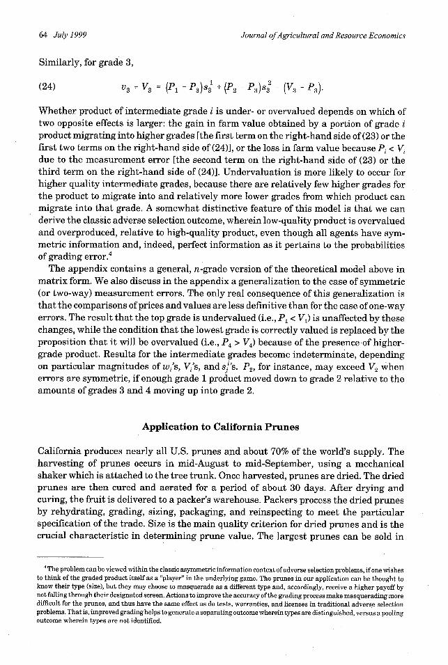
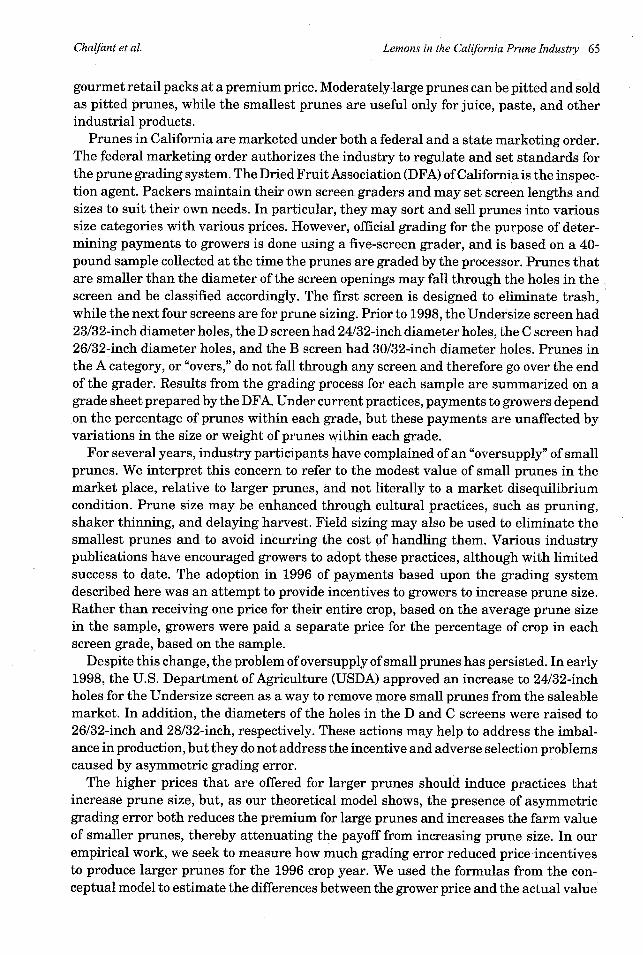
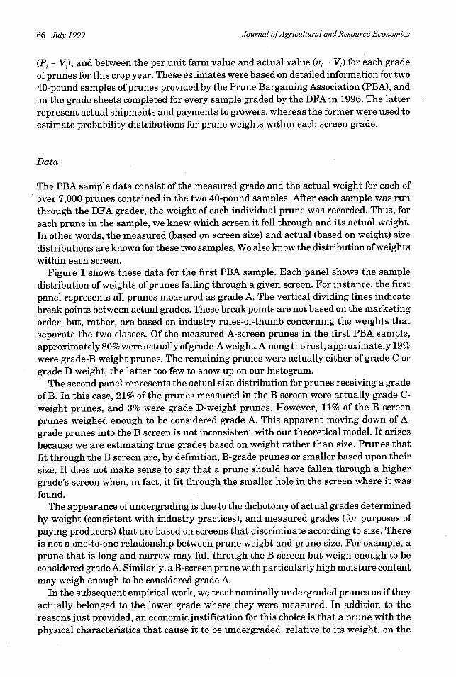
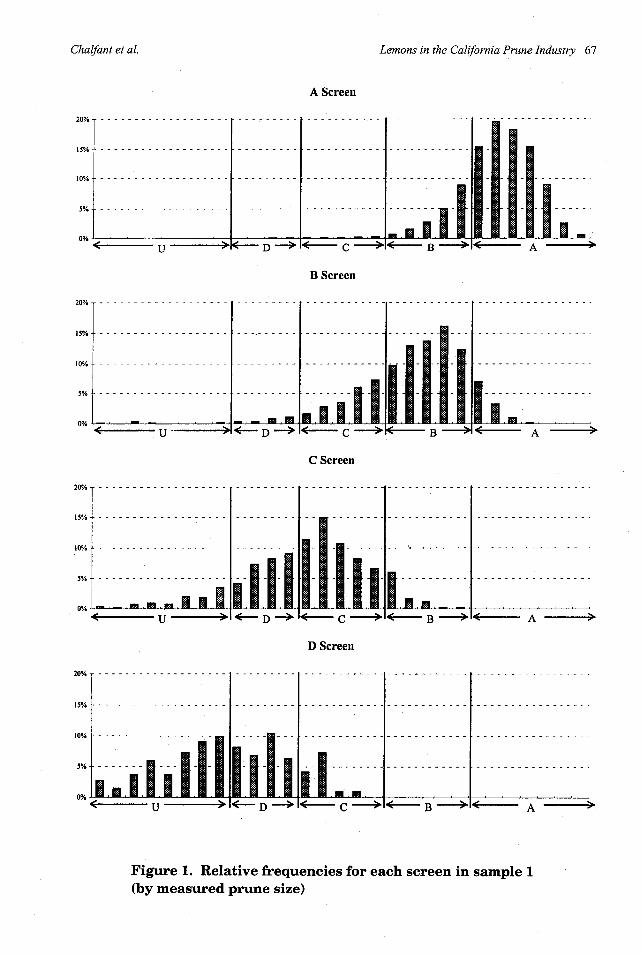
Figure 1 shows these data for the first PBA sample. Each panel shows the sampledistribution of weights of prunes falling through a given screen. For instance, the first

panel represents all prunes measured as grade A. The vertical dividing lines indicate

break points between actual grades. These break points are not based on the marketing

order, but, rather, are based on industry rules-of-thumb concerning the weights thatseparate the two classes. Of the measured A-screen prunes in the first PBA sample,

approximately 80% were actually of grade-A weight. Among the rest, approximately 19%were grade-B weight prunes. The remaining prunes were actually either of grade C or

grade D weight, the latter too few to show up on our histogram.The second panel represents the actual size distribution for prunes receiving a grade

of B. In this case, 21% of the prunes measured in the B screen were actually grade C-weight prunes, and 3% were grade D-weight prunes. However, 11% of the B-screenprunes weighed enough to be considered grade A. This apparent moving down of A-grade prunes into the B screen is not inconsistent with our theoretical model. It arisesbecause we are estimating true grades based on weight rather than size. Prunes that

fit through the B screen are, by definition, B-grade prunes or smaller based upon theirsize. It does not make sense to say that a prune should have fallen through a highergrade's screen when, in fact, it fit through the smaller hole in the screen where it wasfound.

The appearance of undergrading is due to the dichotomy of actual grades determined

by weight (consistent with industry practices), and measured grades (for purposes of

paying producers) that are based on screens that discriminate according to size. Thereis not a one-to-one relationship between prune weight and prune size. For example, aprune that is long and narrow may fall through the B screen but weigh enough to beconsidered grade A. Similarly, a B-screen prune with particularly high moisture contentmay weigh enough to be considered grade A.

In the subsequent empirical work, we treat nominally undergraded prunes as if theyactually belonged to the lower grade where they were measured. In addition to the

reasons just provided, an economic justification for this choice is that a prune with the

physical characteristics that cause it to be undergraded, relative to its weight, on the

66 July 1999

Chalfant et al. Lemons in the California Prune Industry 67

A Screen

20% - - - - - - - - - - - -

15% t - - - - - - - - - - -I - - - -- -- -- - - - - - - - - -- - - -- - - - - - - - - - - - - -1- - - - - - - - - - -

0 L--- ------ ---- - - ---

O% -- U -- > D -< C - - B- A --

B Screen

20% -- ------------------- ----- ---- ------------------------ - ----------------

10% --- -------------- - --------- -------- ---- - -- ----- ------- ---

o0%

< U ---- " "- - D > < C > < B ' < A

C Screen

20% ------------------- ---------.--- --------------------- -----------------

15% .. ------------------- --------- - - ------------------- -----------------

10./, --------------------- ------- -. -l -g - - - -----.----- -----------------

10%......... .......... | | |<-- U ---- > <- D <--- C -> < B > <i A -- >

D Screen

20% .-------------------- --------------------------------- -----------------

15% 0..----...----........-.. ---.---.---------...-.-------..-.---------.-..-.

5% --- -- - - - - - |- - - - - -------------------- -----------------

0%/.

< U- >< D > -- C > B > < A >

Figure 1. Relative frequencies for each screen in sample 1(by measured prune size)

Journal of Agricultural and Resource Economics

DFA grader would also tend to reduce its grade on a processor's grading system, because

both are based on size rather than weight. Because end use and wholesale value of aprune are determined by the processors' grades, such prunes would be used and valuedas if they were in fact of the lower grade. Allowing for undergrading-by defining gradesusing weight and allowing for symmetric grading errors, rather than reclassifying theprunes in question-did not materially affect the results of the empirical analysis.Modified versions of tables 1-5 that allow prunes to be undergraded are available fromthe authors upon request. 5

The shipments data represent the grading sheets for 1,487 actual shipments from the1996 crop year. Each sheet reports the total weight and the average size in each of themeasured grades A, B, C, D, and U, based on the 40-pound sample taken from eachshipment after drying. With only the total weight of prunes in each screen grade, wecannot determine the extent to which grading error is present in any particularshipment. We used the PBA samples to estimate theoretical size distributions for eachgrade, which we then applied to the shipments data, as discussed below.

Estimation of Prune Size Distributions

Because the actual and measured distributions of the two 40-pound samples are known,this information was used to infer the actual size distributions for each of the 1,487actual shipments. Based on analysis of the sample data, it appeared reasonable to modelthe size distributions for the prunes, within each measured grade, using the Gammaprobability distribution, which allows for an asymmetry in the distribution of prunesizes.6 A unique Gamma distribution for the weights of individual prunes was estimatedfor each measured grade in each shipment. Because we had only summary informationon the weight within each grade, it was necessary to use prior information to identifythe two parameters of the distribution. We chose to assume that the coefficient ofvariation within each measured grade was the same as for our two detailed samplescombined.

This coefficient of variation was used in conjunction with the reported average prunesize to estimate the two parameters for the Gamma distribution for each grade of each1996 shipment. The Gamma probability density function is written as

(25) f(x) = - e-(x/P a-1, X > 0,r(a)a

where r(a) denotes the usual Gamma function, and the mean and variance are ua andaC2 , respectively (e.g., Mittelhammer, p. 187). We can infer the value of the a parameterbased on the coefficient of variation (CV) observed in each grade:

5 An alternative empirical approach would be to define true grade based on size rather than weight. For example, theindividual prunes in the PBA sample could, in principle, have been measured for size rather than for weight. "True" sizewould then be the smallest screen size the prune could physically fit through. Deviations of measured screen from true screenwould necessarily be one-way, or asymmetric, in this analysis. We must use weight as a proxy for true screen size becausewe have no such data concerning the physical dimensions of individual prunes.

6 Goodness-of-fit tests supported the Gamma, relative to the log-normal or Beta distributions, which also have the desiredasymmetry.

68 July 1999


(26) CV2 2 _a2 _

(4 (a)2 a

Hence, we set

(27) a=(CV) 2

We then estimated the p parameter by setting the average size in each grade-shipmentcombination equal to its theoretical expected value, ap, and solving for P using the athat was based on the CV.

Thus, for each shipment, we have a set of estimated probability distributions from theGamma(a,P) family describing the probability distribution of weights of individualprunes in each measured grade. By evaluating the estimated cumulative distributionfunction at the break points between actual grades, we were able to estimate the propor-tions of prunes of an actual grade that were measured in each of the five grades. Theaverages of these proportions over all 1996 shipments are reported in tables 1 and 2.

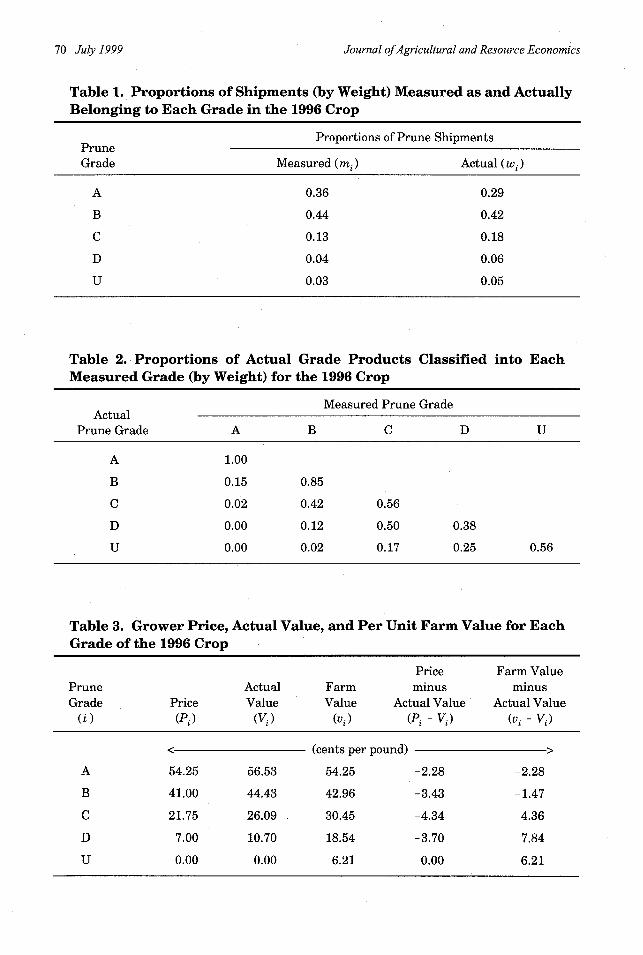
Table 1 contains mi and wi, the measured and actual proportions of prunes in a grade,for each grade, averaged over all shipments of the 1996 crop. Differences between theactual and measured proportions are readily apparent, but the degree of measurementerror is further clarified in table 2. Each row of table 2 refers to the actual prune gradeand each column refers to the measured prune grade. Cells contain sj, the proportionof the prunes actually belonging to rowj's grade that received column i's grade, so thatthe diagonal elements represent proportions of correctly graded prunes. The numbersbelow the diagonal represent the percentage of prunes of each actual grade migratingto higher grades.

Table 2 shows that the probability of grading errors is greatest in the lower grades.This result is not surprising, because products in these grades have the greatestopportunity to migrate into higher grades, as shown in the conceptual model. AllA-quality prunes are graded correctly by construction of the grading process, and 85%of B-quality prunes are graded correctly, with the remaining 15% masquerading asA-quality prunes. However, only 56% of C-quality prunes are graded correctly, with 42%masquerading as B prunes and 2% masquerading as A prunes. Only 38% of trueD-quality prunes were graded as D, with 50% and 12% migrating into the C and Bscreens, respectively.

Tables 1 and 2 contain the grading information necessary to specify equations (1)-(4).The grower prices for each grade, based on the outcome of negotiations between thehandlers and the PBA, are presented in table 3. This information, along with thegrading information in tables 1 and 2, is sufficient for specifying equations (5)-(8) andequations (19)-(22), and solving for the actual value of each grade (Vi) and average perunit farm values (vi). These values are included in table 3, as are the Pi - Vi differentialsand the average vi - Vi differentials for each grade. All grades are undervalued, exceptfor the lowest grade U (undersized), i.e., the price spread is negative, meaning that thegrower price is lower than the actual value of prunes of grades A through D. The priceof grade A prunes is lower than its true value by 2.3¢/pound (or by 4%), while B-gradeprunes are undervalued by 3.4¢/pound (or 8%). By construction, the grower price for theU grade exactly equals its true value, zero.

Chalfant et al.


Table 1. Proportions of Shipments (by Weight) Measured as and ActuallyBelonging to Each Grade in the 1996 Crop

Proportions of Prune ShipmentsPruneGrade Measured (mi) Actual (wi)

A 0.36 0.29

B 0.44 0.42

C 0.13 0.18

D 0.04 0.06

U 0.03 0.05

Table 2. Proportions of Actual Grade Products Classified into EachMeasured Grade (by Weight) for the 1996 Crop

Measured Prune GradeActual

Prune Grade A B C D U

A 1.00

B 0.15 0.85

C 0.02 0.42 0.56

D 0.00 0.12 0.50 0.38

U 0.00 0.02 0.17 0.25 0.56

Table 3. Grower Price, Actual Value, and Per Unit Farm Value for EachGrade of the 1996 Crop

Price Farm ValuePrune Actual Farm minus minusGrade Price Value Value Actual Value Actual Value

(i (P) (Vi) (Vi) (Pi - Vi (vi - Vi)

< (cents per pound) >

A 54.25 56.53 54.25 -2.28 -2.28

B 41.00 44.43 42.96 -3.43 -1.47

C 21.75 26.09 30.45 -4.34 4.36

D 7.00 10.70 18.54 -3.70 7.84

U 0.00 0.00 6.21 0.00 6.21

70 July 1999


The average spread between the per unit farm value and the actual value of prunesin each grade is shown in the last column of table 3. Since A-grade prunes cannotmasquerade as other grades, their per unit farm value equals their grower price, andthus differs from their true value by the same amount as the price, 2.3¢/pound. ForB-grade prunes, the average per unit farm value is 3% lower than the actual value. Thisnegative spread indicates that the downward adjustment in grower prices due tomeasurement error decreases the average revenue earned on B-grade prunes more thanthe masquerading of B-grade prunes as A-grade prunes increases it. This relationshipis reversed for grades C, D, and U, for which per unit grower revenue is larger than theactual value. Here, the increase in revenue from each grade masquerading as highergrades outweighs the decrease in revenue resulting from lower grower prices. Onaverage, grade C and D prunes earn per unit farm values of 17% and 73%, respectively,in excess of their true values. Furthermore, undersized prunes, which have no value,earn over 6¢/pound solely due to measurement error.

Distribution Effects of Grading Error

The preceding calculations describe the effects of grading error on different grades ofprunes. A different set of calculations concerns the distribution effects of grading erroracross producers. The errors in valuation of the form Pi - Vi will be the same for everygrower, since the Vi's are calculated based on industry averages for the wi's, mi's, andsJ's. However, the per unit farm values will vary between shipments, to the extent thatany of these parameters depart from industry averages.

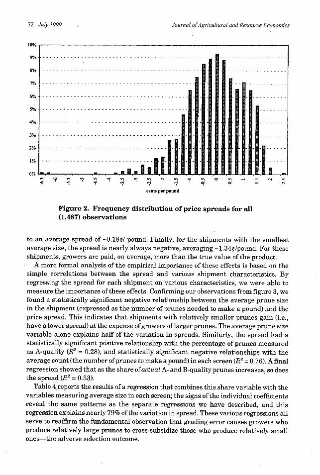
We calculated a measure of the value-price "spread" for every shipment, defined asthe difference between the total value per unit of the shipment across all grades and thetotal revenue per unit received by the grower. A positive value for the spread representsthe rent captured by the processor for that shipment effectively or, alternatively, valuenot captured by the grower. Conversely, a negative spread would indicate revenueearned by the grower in excess of the true value of the shipment. Our analysis indicatesthat a shipment with relatively large prunes should have a positive spread, while onewith predominately small prunes will have a negative spread due, for example, to therelatively larger effect on payments of C-quality prunes receiving the price for B's.

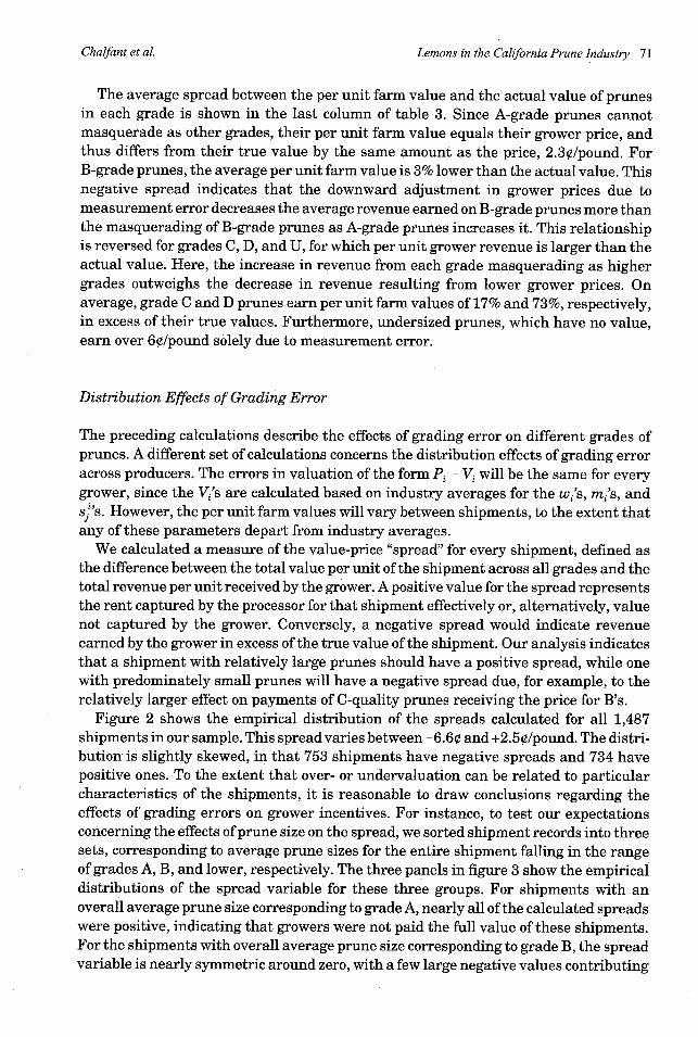
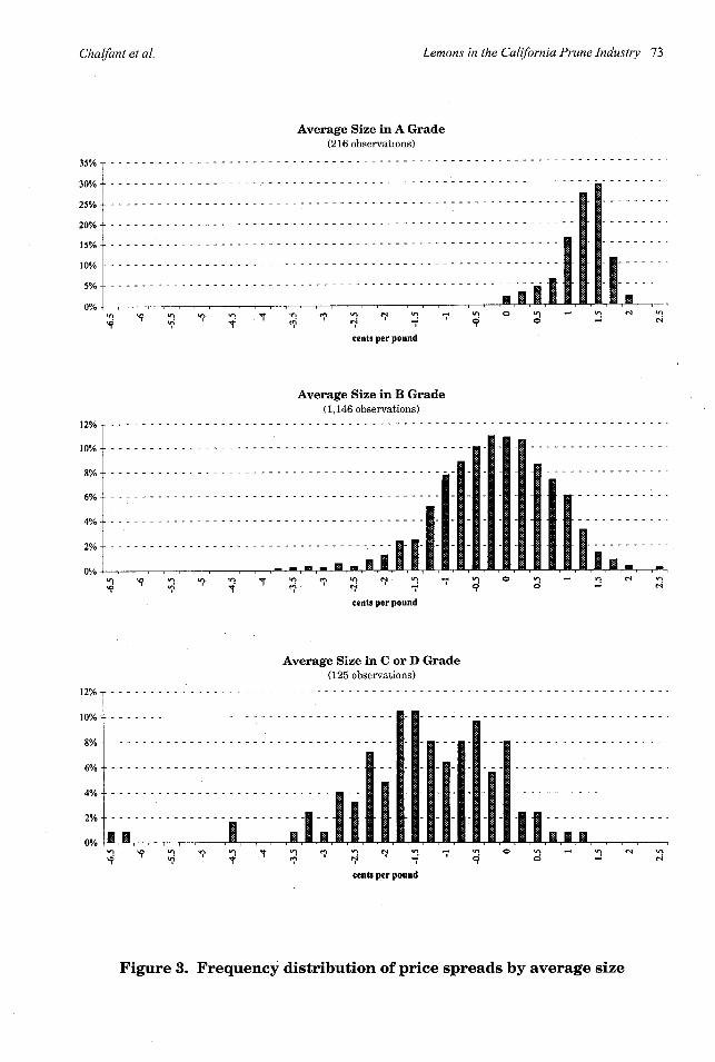
Figure 2 shows the empirical distribution of the spreads calculated for all 1,487shipments in our sample. This spread varies between - 6.6¢ and +2.5¢/pound. The distri-bution is slightly skewed, in that 753 shipments have negative spreads and 734 havepositive ones. To the extent that over- or undervaluation can be related to particularcharacteristics of the shipments, it is reasonable to draw conclusions regarding theeffects of grading errors on grower incentives. For instance, to test our expectationsconcerning the effects of prune size on the spread, we sorted shipment records into threesets, corresponding to average prune sizes for the entire shipment falling in the rangeof grades A, B, and lower, respectively. The three panels in figure 3 show the empiricaldistributions of the spread variable for these three groups. For shipments with anoverall average prune size corresponding to grade A, nearly all of the calculated spreadswere positive, indicating that growers were not paid the full value of these shipments.For the shipments with overall average prune size corresponding to grade B, the spreadvariable is nearly symmetric around zero, with a few large negative values contributing

Chalfant et al.


9%

8%

7%

6%

5%

4%

3%

2%

1%

0%1

\s VI VS X V) C n v I _ | O -r

cents per pound

Figure 2. Frequency distribution of price spreads for all(1,487) observations

to an average spread of -0.18¢/ pound. Finally, for the shipments with the smallestaverage size, the spread is nearly always negative, averaging -1.34¢/pound. For theseshipments, growers are paid, on average, more than the true value of the product.

A more formal analysis of the empirical importance of these effects is based on thesimple correlations between the spread and various shipment characteristics. Byregressing the spread for each shipment on various characteristics, we were able tomeasure the importance of these effects. Confirming our observations from figure 3, wefound a statistically significant negative relationship between the average prune sizein the shipment (expressed as the number of prunes needed to make a pound) and theprice spread. This indicates that shipments with relatively smaller prunes gain (i.e.,have a lower spread) at the expense of growers of larger prunes. The average prune sizevariable alone explains half of the variation in spreads. Similarly, the spread had astatistically significant positive relationship with the percentage of prunes measuredas A-quality (R2 = 0.28), and statistically significant negative relationships with theaverage count (the number of prunes to make a pound) in each screen (R2 = 0.76). A finalregression showed that as the share of actual A- and B-quality prunes increases, so doesthe spread (R2 = 0.33).

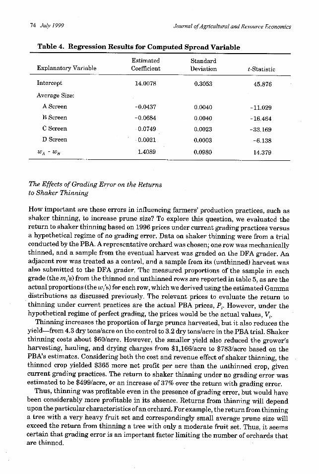
Table 4 reports the results of a regression that combines this share variable with thevariables measuring average size in each screen; the signs of the individual coefficientsreveal the same patterns as the separate regressions we have described, and thisregression explains nearly 79% of the variation in spread. These various regressions allserve to reaffirm the fundamental observation that grading error causes growers whoproduce relatively large prunes to cross-subsidize those who produce relatively smallones-the adverse selection outcome.

I- ~~t--I--------

----- --- -----. - ----- - - - - - - - - 1-1- -

_-- - - - - - - - - - - - - - - - - -.-

I An.

------------ ------ -----

------------------------------------------------- -------------------

---------------------------------------------- -----------------

I

- - -- - - - - - - - - - - - - - - - - --- -" '- -- - - - - -

I- I I I

- - - - - - - - - - -

- - - - - - - - - - -

- - - - - - - - - - -

- - - - - - - - - -

- - - - - - - -

f I -- , I- I ------ In

I

72 July 1999

Chalfant et al. Lemons in the California Prune Industry 73

Average Size in A Grade(216 observations)

35%

30%

25%-- - - -

20%

50% -------------------------------------------------- - - --- - - - - -

10%

5%

0% . ' ' T? n m X ^I ^ n vI -4 O N _ *

m

cents per pound

Average Size in B Grade(1,146 observations)

10% -- -- ------------------------------------ - - - ---

6% -- - - - - - - - - - - - - - - - - - - - - - - - - - - - - - - - - - - - - - - - - - - - --- --------

o0% -

In° , , n v, _i, pr , !S ! v! o oI _4 T ! in

cents per pound

Average Size in C or D Grade(125 observations)

cents per pound

Figure 3. Frequency distribution of price spreads by average size

1

I


Table 4. Regression Results for Computed Spread Variable

Estimated StandardExplanatory Variable Coefficient Deviation t-Statistic

Intercept 14.0078 0.3053 45.876

Average Size:

A Screen -0.0437 0.0040 -11.029

B Screen -0.0684 0.0040 -16.464

C Screen -0.0749 0.0023 -33.169

D Screen -0.0021 0.0003 -6.138

WA + WB 1.4089 0.0980 14.379

The Effects of Grading Error on the Returnsto Shaker Thinning

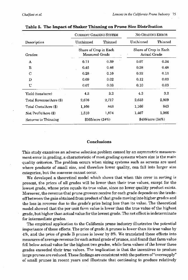
How important are these errors in influencing farmers' production practices, such asshaker thinning, to increase prune size? To explore this question, we evaluated thereturn to shaker thinning based on 1996 prices under current grading practices versusa hypothetical regime of no grading error. Data on shaker thinning were from a trialconducted by the PBA. A representative orchard was chosen; one row was mechanicallythinned, and a sample from the eventual harvest was graded on the DFA grader. Anadjacent row was treated as a control, and a sample from is (unthinned) harvest wasalso submitted to the DFA grader. The measured proportions of the sample in eachgrade (the mi's) from the thinned and unthinned rows are reported in table 5, as are theactual proportions (the wi's) for each row, which we derived using the estimated Gammadistributions as discussed previously. The relevant prices to evaluate the return tothinning under current practices are the actual PBA prices, Pi. However, under thehypothetical regime of perfect grading, the prices would be the actual values, Vi.

Thinning increases the proportion of large prunes harvested, but it also reduces theyield-from 4.3 dry tons/acre on the control to 3.2 dry tons/acre in the PBA trial. Shakerthinning costs about $60/acre. However, the smaller yield also reduced the grower'sharvesting, hauling, and drying charges from $1,166/acre to $783/acre based on thePBA's estimates. Considering both the cost and revenue effect of shaker thinning, thethinned crop yielded $365 more net profit per acre than the unthinned crop, givencurrent grading practices. The return to shaker thinning under no grading error wasestimated to be $499/acre, or an increase of 37% over the return with grading error.

Thus, thinning was profitable even in the presence of grading error, but would havebeen considerably more profitable in its absence. Returns from thinning will dependupon the particular characteristics of an orchard. For example, the return from thinninga tree with a very heavy fruit set and correspondingly small average prune size willexceed the return from thinning a tree with only a moderate fruit set. Thus, it seemscertain that grading error is an important factor limiting the number of orchards thatare thinned.

74 July 1999


Table 5. The Impact of Shaker Thinning on Prune Size Distribution

CURRENT GRADING SYSTEM NO GRADING ERROR

Description Unthinned Thinned Unthinned Thinned

Share of Crop in Each Share of Crop in EachGrades: Measured Grade Actual Grade

A 0.11 0.39 0.07 0.34

B 0.45 0.46 0.38 0.48

C 0.28 0.10 0.32 0.13

D 0.09 0.02 0.12 0.03

U 0.07 0.03 0.10 0.03

Yield (tons/acre) 4.3 3.2 4.3 3.2

Total Revenue/Acre ($) 2,676 2,717 2,633 2,809

Total Costs/Acre ($) 1,166 843 1,166 843

Net Profit/Acre ($) 1,510 1,874 1,467 1,966

Returns to Thinning $365/acre (24%) $499/acre (34%)

Conclusions

This study examines an adverse selection problem caused by an asymmetric measure-

ment error in grading, a characteristic of most grading systems where size is the main

quality criterion. The problem occurs when sizing systems such as screens are used

where products of small size, and therefore lower quality, can fall into larger size

categories, but the converse cannot occur.We developed a theoretical model which shows that when this error in sorting is

present, the prices of all grades will be lower than their true values, except for the

lowest grade, whose price equals its true value, since no lower quality product exists.

Moreover, the revenue that prune growers receive for each grade depends on the trade-

off between the gain obtained from product of that grade moving into higher grades and

the loss in revenue due to the grade's price being less than its value. The theoretical

model showed that the per unit farm value is lower than the true value of the highest

grade, but higher than actual value for the lowest grade. The net effect is indeterminatefor intermediate grades.

The empirical application to the California prune industry illustrates the potential

importance of these effects. The price of grade A prunes is lower than its true value by

4%, and the price of grade B prunes is lower by 8%. We translated these effects into

measures of average revenue for each actual grade of prunes, and found that farm value

fell below actual value for the highest two grades, while farm values of the lower three

grades exceeded their true values. The implication is that the incentives to produce

large prunes are reduced. These findings are consistent with the pattern of "oversupply"of small prunes in recent years and illustrate that continuing to produce relatively

Chalfant et al.


greater numbers of small prunes, rather than undertaking shaker thinning or othercultural practices to produce larger prunes, may well be a rational response to currentincentives. The industry can partially address the problem of oversupply of small prunesby improving the accuracy of the grading process. Examples would include increasingscreen length or adding additional screens on the DFA grader. Alternatively, theindustry might consider a graduated payment system that offers premiums anddiscounts based on average prune size in each measured grade, rather than a singleprice per grade, as is the current practice.

[Received October 1998; final revision received April 1999.]

References

Akerlof, G. "The Market for 'Lemons': Qualitative Uncertainty and the Market Mechanism." Quart. J.Econ. 84,3(1970):488-500.

Bierlen, R., and 0. Grunewald. "Price Incentives for Commercial Fresh Tomatoes." J. Agr. and Appl.Econ. 27,1(1995):138-48.

De, S., and P. Nabar. "Economic Implications of Imperfect Quality Certification." Econ. Letters 37,1(1991):333-37.

Giannakas, K., R. Gray, and N. Lavoie. "The Impact of Protein Increments on Blending Revenues in theCanadian Wheat Industry." Internat. Advances in Econ. Res. 5(1999, in press).

Heinkel, R. "Uncertain Product Quality: The Market for Lemons with an Imperfect Testing Technology."Bell J. Econ. 12,2(1981):625-36.

Henderson, S. M., and R. L. Perry. Agricultural Process Engineering. Westport CT: AVI Publishing Co.,1976.

Hennessy, D. A. "The Economics of Purifying and Blending." S. Econ. J. 63,1(1996a):223-32.. "Information Asymmetry as a Reason for Food Industry Vertical Integration." Amer. J. Agr.

Econ. 78,4(1996b):1034-43.Hennessy, D. A., and T. I. Wahl. "Discount Schedules and Grower Incentives in Grain Marketing."

Amer. J. Agr. Econ. 79,3(1997):888-901.Lichtenberg, E. "The Economics of Cosmetic Pesticide Use." Amer. J. Agr. Econ. 79,1(1997):39-46.Mason, C. F., and F. P. Sterbenz. "Imperfect Product Testing and Market Size." Internat. Econ. Rev.

35,1(1994):61-86.Matsumoto, M., and B. C. French. "Empirical Determination of Optimum Quality Mix."Agr. Econ. Res.

23,1(1971):1-9.Mittelhammer, R. C. Mathematical Statistics for Economics and Business. New York: Springer-Verlag

New York, Inc., 1996.Naik, G. "Price-Quality Relationships in Raw Silk Markets." Indian Econ. Rev. 30,1(1995):101-19.Starbird, S. A. "The Effect of Quality Assurance Policies for Processing Tomatoes on the Demand for

Pesticides." J. Agr. and Resour. Econ. 19,1(1994):78-88.

76 July 1999


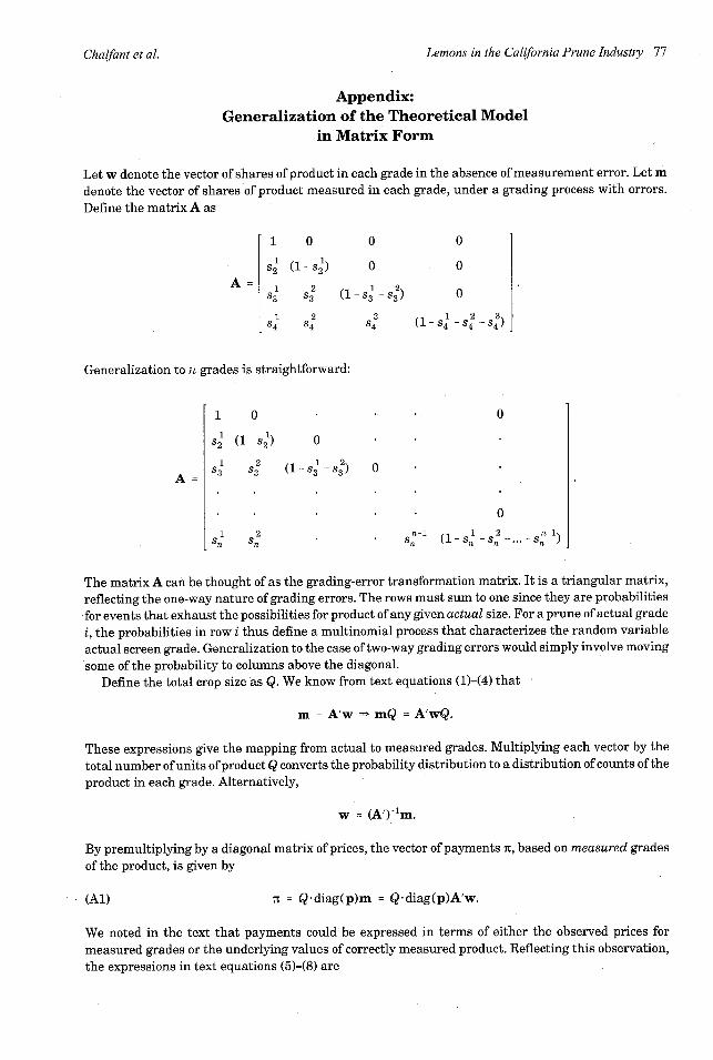
Appendix:Generalization of the Theoretical Model

in Matrix Form

Let w denote the vector of shares of product in each grade in the absence of measurement error. Let m

denote the vector of shares of product measured in each grade, under a grading process with errors.

Define the matrix A as

1 0 0 01

S2 (1- S2) 0 0

A 1 2 1 2sA s 2 (1-s3-sO) 0

1 2 3 ( 1 2 384 4 s4 (1- 4 -4 -8 4

Generalization to it grades is straightforward:

A

1 0 * 0

s2 (1- s 1) 0

1 2s3 s3 (1-s -s ) 0

1 2 nl 2 n-lSn Sn S n(1-S -s - s )

The matrix A can be thought of as the grading-error transformation matrix. It is a triangular matrix,

reflecting the one-way nature of grading errors. The rows must sum to one since they are probabilities

for events that exhaust the possibilities for product of any given actual size. For a prune of actual grade

i, the probabilities in row i thus define a multinomial process that characterizes the random variableactual screen grade. Generalization to the case of two-way grading errors would simply involve moving

some of the probability to columns above the diagonal.Define the total crop size as Q. We know from text equations (1)-(4) that

m = A'w = mQ = A'wQ.

These expressions give the mapping from actual to measured grades. Multiplying each vector by the

total number of units of product Q converts the probability distribution to a distribution of counts of the

product in each grade. Alternatively,

w = (A')-m.

By premultiplying by a diagonal matrix of prices, the vector of payments nT, based on measured grades

of the product, is given by

(Al) 7t = Qdiag(p)m = Q diag(p)A'w.

We noted in the text that payments could be expressed in terms of either the observed prices formeasured grades or the underlying values of correctly measured product. Reflecting this observation,the expressions in text equations (5)-(8) are

Chalfant et al.

.

i


diag(m)p = A'diag(w)V

or

(A2) p = [diag(m)]-1A'diag(w)V.

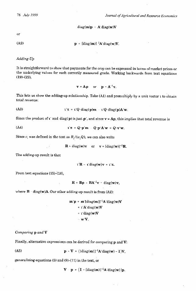
Adding-Up

It is straightforward to show that payments for the crop can be expressed in terms of market prices orthe underlying values for each correctly measured grade. Working backwards from text equations(19)-(22),

v = Ap or p =A-1 v.

This lets us show the adding-up relationship. Take (Al) and premultiply by a unit vector i to obtaintotal revenue:

(A3) tI't = t'Qdiag(p)m = t'Q diag(p)A'w.

Since the product of ' and diag(p) is just p', and since v = Ap, this implies that total revenue is

(A4) l't = Q-p'm = Q'p'A'w = Q-v'w.

Since vi was defined in the text as Ri/(wiQ), we can also write

R = diag(w)v or v = [diag(w)]-lR.

The adding-up result is that

'R = i'diag(w)v = l'n.

From text equations (15)-(18),

R = Bp = BA-v = diag(w)v,

where B = diag(w)A. Our other adding-up result is from (A2):

m'p = m'[diag(m)]-lA'diag(w)V

= 'A'diag(w)V

= 'diag(w)V

= w'V.

Comparing p and V

Finally, alternative expressions can be derived for comparing p and V:

(A5) p - V= ([diag(m)]- A'diag(w)- I)V,

generalizing equations (5) and (9)-(11) in the text, or

V - p = (I - [diag(m)]-1A'diag(w))p.

78 July 1999


Symmetric Errors

We used the assumption that the A matrix is triangular, reflecting asymmetric grading errors, indeveloping the results in the text in a recursive manner. However, the expressions in this appendix donot require that particular structure for A. Each result holds for the case of the two-way or symmetricgrading errors. The key in either case is to think of the mapping from m to w as a simple linearredefinition of the number of units of the product in various grades. As long as this is understood, it isa matter of indifference how prices are expressed for a given crop.

Our interest is in the effect of grading errors on the share of revenues accruing to each measuredgrade, and how grading error affects the differences between actual values and market prices formeasured grades. In equation (A5) above, since the A matrix has no zero elements in the first column,the first row of its transpose has no zero elements, and the equation for P1 - V1 is unaffected by makingerrors symmetric (except that the 1 on the diagonal will be reduced, to the extent that grade 1 productmoves down in grade). For each comparison between P and V for other grades, additional terms willappear in the generalizations of equations (5) and (12)-(14) from the text. For instance, for grade 2,there now will be a term involving V1, since the 0 appearing in the first row and second column of A isreplaced by a positive fraction. This reflects the possible appearance of grade 1 product in measuredgrade 2, which raises the average value of that grade-making the comparison between P2 and V2ambiguous, whereas it was clear that P < V2 for the asymmetric case. Similar results apply for theother intermediate grades. For the lowest grade, which can now include higher-grade product, equation(5) in the text is replaced with the result that P4 > V4.

Chalfant et al.

Asymmetric Grading Error and Adverse Selection:...

Documents

Transcript of Asymmetric Grading Error and Adverse Selection:...